Noise due to neutral modes in the $\nu=2/3$ fractional quantum Hall state

Abstract

We theoretically study charge noise generated by excited neutral modes, which impinge on the quantum point contact of a quantum Hall bar with filling fraction $\nu=2/3$. The noise is computed for thermally excited neutral modes as well as for biased neutral modes with dipole-fermion excitations. Within the dipole-fermion picture, we show that the noise arising from two colliding modes can be suppressed due to Pauli-blocking and be non-universal due to random edge disorder, but becomes universal upon disorder-averaging. The ratio of noise due to two colliding neutral modes and noise due to only one such mode is smaller for dipole-fermions than for thermal excitations, thus providing evidence for the different quantum statistics of the two types of excitations.

The behavior of two-dimensional (2D) electron gases in the fractional quantum Hall (FQH) regime has garnered much attention ever since its discovery Tsui et al. (1982). While FQH liquids are incompressible with finite energy gaps to all bulk excitations, they support one or more 1D gapless conducting channels along their boundaries Wen (1991). The edges of some FQH states, such as the spin-polarized $\nu=2/3$ Kane et al. (1994) and the $\nu=5/2$ Pfaffian and anti-Pfaffian non-Abelian states Levin et al. (2007); Lee et al. (2007), are predicted to possess neutral modes which can carry heat but no charge. The Majorana degree of freedom in the (anti-)Pfaffian neutral mode is essential for the non-Abelian statistics of these states. For the case of $\nu=2/3$, our focus in this paper, the neutral mode flows opposite to the charge mode. While the existence of neutral modes was first predicted almost 20 years ago Kane et al. (1994); Kane and Fisher (1995), experimental evidence for their existence was obtained only recently using shot noise measurements nme ; Dolev et al. (2011); Gross et al. (2012) and quantum dot thermometers Venkatachalam et al. (2012); Altimiras et al. (2012).

In an abelian FQH state with two edge channels, the neutral mode is the dipole excitation of the composite edge — made of charges with opposite signs on the two edge channels. Theoretically, for the specific example of the random 2/3-edge the neutral mode is made of spinful chiral fermions  Kane et al. (1994); Kane and Fisher (1995). Its excitations may be expressed as spin flips of these fermions. In the presence of disorder, the number of these excitations is not conserved, since the scattering of an electron from the $\nu=1$ mode to the counter-propagating $\nu=1/3$ mode creates such a spin flip excitation in the neutral mode. While neutral mode heat transport can be partially understood in terms of thermaly excitated bosonic collective modes, we focus here on possible manifestations of the fermionic nature of the neutral mode. We refer to the fermions as “dipole fermions”.

In this letter, we address the question how neutral mode dipole-fermion excitations and their interaction with a QPC can be described theoretically, and we identify signatures of their quantum statistics in a setup where two biased neutral modes collide at a QPC. By drawing on an analogy with the effect of a current bias on edge correlation functions of the charge mode, we associate an oscillatory behavior of neutral mode edge correlation functions with a biased neutral mode. To quantify our findings, we introduce the ratio $\gamma$ between the current noise at a QPC due to two colliding neutral modes and the current noise due to only one impinging neutral mode. We find that for biased neutral modes, $\gamma$ is not only smaller than two, but it is also much smaller than for the case of colliding thermally excited neutral modes. This result is a fingerprint of quantum statistics. It originates from a partial Pauli-blockade of occupied states, and also allows to experimentally distinguish dipole-fermion excitations from thermaly excitated neutral modes. Our heuristic description of biased neutral modes is backed up by a full-fledged Keldysh calculation, and a comparison of our theoretical results with the recent experiment Gross et al. (2012) suggests that the collision of thermally excited neutral modes was observed there.

General discussion of shot noise versus thermal noise : Before delving into detailed calculations, we first present a simple interpretation of noise generation due to thermal excitations and a current bias, respectively. For now, it suffices to consider a QH bar in the $\nu=1$ quantum Hall state as shown in Fig. 1, and focus on the dc current noise arising at the QPC due to stochastic backscattering of quasi-particles there. In order to make connection with the discussion of fractional edges to follow, the modes on the two edges are described by two oppositely chiral boson fields with Lagrangian densities $\mathcal{L}_{j}=\partial_{x}\phi_{j}((-)^{j-1}\partial_{t}-u\partial_{x})\phi_{j}/2$, where $j=1,2$ labels the edges and $u$ denotes the edge plasmon velocity. Backscattering at the QPC can be modeled by the tunneling term $\mathcal{L}_{\rm tun}={T}+T^{\dagger}$, with

$${T}\ =\ e^{ieVt}\zeta e^{i\varphi_{1}(x=0,t)-i\varphi_{2}(x=0,t)}\ \ ,$$ (1)

which describes the tunneling of charge $e$ electrons. The exponential factor containing the bias $V$ between upper and lower edge describes the time evolution of electron operators on the upper edge versus those on the lower edge. The current backscattered at the QPC is given by $I_{B}=-ie\hbar^{-1}({T}-{T}^{\dagger})$, and current noise is then obtained from the current-current correlation function $S_{B}(t)=\left\langle I_{B}(t)I_{B}(0)\right\rangle$ via $S_{B}=\int_{-\infty}^{\infty}dtS_{B}(t)$.

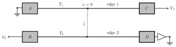
Figure 1: A quantum Hall bar with a single charge mode on each edge. The upper and lower edges are labeled 1 and 2, respectively. The tunneling amplitude between the edges is given by $\zeta$.

Computing the current correlation function to leading order in the backscattering, the expectation value of the two current operator factorizes into a product of correlation functions of the quasi-particle operator evaluated on the same edge,

$$S^{0}_{B}(t)=e^{2}|\zeta|^{2}\cos(eVt)F_{1}(T_{1},t)F_{1}(T_{2},t)/2$$ (2)

where $F_{1}(T_{j},t)=\langle e^{i\varphi_{j}(x=0,t)}e^{-i\varphi_{j}(x=0,0)}\rangle$ is the finite temperature “greater” correlation function of the electron operator.

When the edge modes are at zero temperature and zero bias the dc current noise vanishes. We now show that this happens due to a cancellation of short- and long-time contributions. Under these conditions, $F_{1}(T_{j}=0,t)=\tau_{c}/(\tau_{c}+it)$, where $\tau_{c}$ is a short-time cutoff. The dc noise has a singular contribution from short-time correlations, $S_{B,\,{\rm short}}^{0}=\int_{-\varepsilon}^{\varepsilon}dtS_{B}^{0}(t)$, and another from long-time edge correlations $S_{B,\,{\rm long}}^{0}=(\int_{-\infty}^{-\varepsilon}+\int_{\varepsilon}^{\infty})dtS_{B}^{0}(t)$. Here, $\varepsilon$ has to be taken on the order of $\tau_{c}$, but $\varepsilon>\tau_{c}$ by a numerical factor. In the ground state of the system, the noise vanishes because of a precise cancellation between these two contributions, $S_{B,\,{\rm short}}^{0}+S_{B,\,{\rm long}}^{0}=0$. This can be seen from contour integration in the lower half plane, using a closed contour consisting of the real axis and an “infinite” semicircle around the origin. Since the contour does not contain a singularity, the integral vanishes. Due to the long-time decay $\propto 1/t^{2}$ of the integrand, the integral over the infinite semicircle vanishes, and we obtain the desired cancellation of $S_{B,\,{\rm short}}^{0}$ and $S_{B,\,{\rm long}}^{0}$.

If the long-time behavior of the current correlation function is modified, finite noise can result. In the following, we consider two mechanisms for such a modification, one due to finite temperature and another due to a finite bias voltage. At a finite temperature $T>0$ there is an exponential suppression of long-time correlations according to

$$F_{1}(T,t)={\pi k_{B}T\tau_{c}/\hbar\over\sin[(\pi k_{B}T/\hbar)(\tau_{c}+it)]}\ \ .$$ (3)

For $t\sim 0$, the function essentially remains unchanged from the zero temperature form, but the long-time (i.e. $t>\hbar/k_{B}T$) correlations are now suppressed exponentially. This suppresses the long-time contribution to noise, $S_{B,\,{\rm short}}>-S_{B,\,{\rm long}}$, and non-zero dc noise results.

A finite bias causes an oscillatory behavior of the tunneling operator Eq. (1), and as a consequence gives rise to a temporally-oscillating factor to (2),

$$S_{B}(t)=S^{0}_{B}(t)\cos(\mu t/\hbar)\ \ .$$ (4)

The singular contribution $S_{B,\,{\rm short}}$ coming from $t\sim 0$ is again unaffected by the oscillatory factor, but the oscillations suppress the non-local time correlations and lead as before to non-zero noise. Later on, we will describe the edge correlation function of a biased neutral mode by such an oscillatory factor as well, and relate the frequency of the oscillations to the magnitude of the neutral current. We find that for the case of two excited neutral modes impinging on a QPC from opposite sides, the noise contributions of thermally excited neutral modes add up, reflecting the bosonic character of thermal excitations, while there is a suppression of noise for dipole fermions that impinge from two biased edges at zero temperature, again reflecting the quantum statistics of excitations.

We now extend the above interpretation for noise generation to the $\nu=2/3$ FQH edge. Let us consider impinging an excited neutral mode only on the upper edge. In the presence of a neutral heat current, one assumes that the charge and neutral modes on the edge are fully equilibrated at the QPC. The heated neutral mode raises the temperature of its partner charge mode until the two equilibrate at a common temperature which is above the lower edge base temperature. In analogy with the above discussion, this exponentially suppresses temporal correlations on the upper edge and generates charge noise at the QPC. This thermal mechanism for noise was the basis behind the heat transport picture Takei and Rosenow (2011) previously developed to explain the experiment nme consisting of a single excited neutral mode. Further below, the noise will be rigorously evaluated in the presence of thermally excited neutral modes on both edges.

We may also consider a model for a biased neutral mode, which formally introduces a temporally-oscillating factor in the correlation function for the neutral quasi-particles, just as in Eq. (4). This model corresponds to neutral dipole-fermion excitations, which are the main focus of the present work. Since only the neutral mode is biased, we introduce the oscillatory factor to the correlation function for the neutral mode only and leave the charge sector unperturbed. One may naïvely expect that biased neutral modes alone should not generate charge noise at the QPC. However, since the most relevant tunneling operators for the $\nu=2/3$ edge involve tunneling of quasi-particles which are superpositions of both the charge and neutral modes, an excited neutral mode indeed generates charge noise at the QPC within the dipole-fermion model as well.

It is important to note that neutral dipole-fermions need not be conserved during tunneling, unlike charged Laughlin quasi-particles which are subject to charge conservation. This means that the tunneling Hamiltonian for dipole-fermions allows terms that correspond to the creation or destruction of two quasi-particles on both edges. Ignoring the charge modes for the moment, the Hamiltonian modeling the tunneling of the neutral dipole-fermions can then be written as

$$H_{\rm tun}=\zeta_{1}e^{i\varphi_{\sigma 1}(x=0)-i\varphi_{\sigma 2}(x=0)}+\zeta_{2}e^{i\varphi_{\sigma 1}(x=0)+i\varphi_{\sigma 2}(x=0)}+h.c.\,,$$ (5)

where $\varphi_{\sigma j}$ denotes the phonon field corresponding to the neutral mode on edge $j$. Introducing the oscillatory factors as before via $e^{i\varphi_{\sigma j}(x=0)}\rightarrow e^{i\varphi_{\sigma j}(x=0)}e^{-i\mu_{\sigma j}t/\hbar}$ should generally lead to two types of oscillatory factors in the backscattering noise

$$S_{B}(\tau)\propto S^{0}_{B}(\tau)\left[\cos(\mu_{\sigma}^{-}\tau/\hbar)+\cos(\mu_{\sigma}^{+}\tau/\hbar)\right],$$ (6)

where $\mu_{\sigma}^{\pm}=\mu_{\sigma 1}\pm\mu_{\sigma 2}$, we have assumed $\zeta_{1}=\zeta_{2}$ for simplicity, and $\mu_{\sigma j}$ denotes the bias voltage on edge $j$. The first term in the square brackets, with dependence on $\mu_{\sigma}^{-}$, describes the behavior expected for fermions: due to the Pauli principle, there is no noise if the bias voltages on the two edges are equal. The second term with dependence on $\mu_{\sigma}^{+}$ arises due to the fact that the number of dipole-fermions is not conserved in scattering processes. The presence of both these terms leads to the generation of finite noise for equally biased neural modes, however with a reduced power as compared to the case of thermally excited neutral modes. The reduction of noise power is due to the first term reflecting the quantum statistics of dipole fermions, thus making the reduced noise power of dipole fermions as compared to bosonic thermal excitations a signature of the quantum statistics of neutral dipole-fermions. In the following, we substantiate this result with a more rigorous microscopic calculation.

Dipole picture for noise in the random $\nu=2/3$ state: In the standard theory for the random $\nu=2/3$ FQH edge, interactions and disorder drive the edge to a disorder-dominated fixed-point where the edge reconstructs into a weakly-coupled charge mode propagating downstream and a counter-propagating neutral mode Kane et al. (1994). At the fixed-point, the neutral mode possesses an exact SU(2)-symmetry, and the propagation of the neutral mode can be interpreted as a flow of dipole (i.e. spinor) fermions. The edge disorder randomly rotates the quantization axes of the dipoles as they propagate spatially along the edge.

Let us consider a $\nu=2/3$ QH bar with a single QPC located at $x=0$. The real-time action for the random $\nu=2/3$ edges is given by $S=\sum_{j=1,2}[S_{\rho j}+S_{\sigma j}+S_{{\rm int},j}+S_{{\rm rand},j}]$, where $S_{\rho j}=(4\pi\nu)^{-1}\int dtdx\ \partial_{x}\phi_{\rho j}[(-)^{j-1}\partial_{t}-u_{\rho}\partial_{x}]\phi_{\rho j}$, $S_{\sigma j}=(8\pi)^{-1}\int dtdx\ \partial_{x}\phi_{\sigma j}[(-)^{j}\partial_{t}-u_{\sigma}\partial_{x}]\phi_{\sigma j}$, $S_{{\rm int},j}=(u_{{\rm int},j}/4\pi)\int dtdx\ \partial_{x}\phi_{\rho j}\partial_{x}\phi_{\sigma j}$, and

$$S_{{\rm rand},j}=\int dtdx\ [\xi(x)e^{i\phi_{\sigma j}}+c.c.]\ \ ,$$ (7)

which describes the spatially random rotations of the dipole quantization axes associated with the neutral modes. Here, $\phi_{\rho j}$ and $\phi_{\sigma j}$ are the charge and neutral phonon modes on edge $j$, and the coupling between these modes is given by $u_{{\rm int},j}$. The random edge potential $\xi(x)$ is uncorrelated on lengths scales longer than the mean-free path $\ell_{0}$. The neutral sector $S_{\sigma j}+S_{{\rm rand},j}$ is characterized by a level-one SU(2) current algebra spanned by $e^{\pm i\phi_{\sigma}}$ and $\partial_{x}\phi_{\sigma}$, which transform as $S_{\pm}$ and $S_{z}$ in an SU(2) algebra. Therefore, for $u_{{\rm int},j}=0$, one can map the neutral sector to an SU(2)-invariant fermionic action written in terms of a two-component spinor $\Psi$, and the random term can then be solved using a space-dependent random SU(2) rotation $\tilde{\Psi}(x)=U(x)\Psi(x)$, where $U(x)$ again is uncorrelated on length scales beyond $\ell_{0}$. Although a finite $u_{{\rm int},j}$ breaks the SU(2)-symmetry, the presence of the random potential renders $u_{{\rm int},j}$ irrelevant in the RG sense, and the charge-neutral decoupled random fixed point is stable.

The quasi-particle tunneling at the QPC is described by the three most relevant tunneling operators Kane et al. (1994),

$$e^{i(\phi_{\rho}-\phi_{\sigma})/2},\ e^{i(\phi_{\rho}+\phi_{\sigma})/2},\ e^{i\phi_{\rho}},$$ (8)

where the first two correspond to quasi-particles with charge $e/3$ and the last with charge $2e/3$. As discussed above, we describe the case of biased dipole fermions by multiplying the first two tunneling operators Eq. (8) containing the neutral phonon fields $\mp\phi_{\sigma j}$ with oscillatory terms $\exp(\pm i\mu_{j}t/\hbar)$, thus modeling the generation of noise due to a neutral current bias.

Disorder randomly rotates the dipole quantization axes of the neutral modes over spatial length scales set by $\ell_{0}$. The noise generated by the neutral modes will depend on the orientations of the polarization axes at the QPC. Since $e^{\pm i\phi_{\sigma}}$ represent spin-one excitations $S_{\pm}$ in an SU(2) algebra, the $e^{\pm i\phi_{\sigma}/2}$ create spin-half objects and form a basis for the 2D representation for SU(2). At the tunneling site, $e^{\pm i\phi_{\sigma}/2}$ then transforms as

$$\left(\begin{array}[]{c}e^{i\phi_{\sigma j}/2}\\ e^{-i\phi_{\sigma j}/2}\end{array}\right)=\left(\begin{array}[]{cc}e^{i\varphi_{j}}\alpha_{j}&e^{i\varphi_{j}}\beta_{j}\\ -e^{-i\varphi_{j}}\beta_{j}&e^{-i\varphi_{j}}\alpha_{j}\end{array}\right)\left(\begin{array}[]{c}e^{i\tilde{\phi}_{\sigma j}/2}\\ e^{-i\tilde{\phi}_{\sigma j}/2}\end{array}\right),$$ (9)

where $\alpha_{j}=\cos(\theta_{j}/2)$ and $\beta_{j}=\sin(\theta_{j}/2)$, and $\theta_{j}$ and $\varphi_{j}$ are the polar and azimuthal angles for edge $j$ at the QPC. After implementing this rotation on the tunneling operators (8), the backscattering correction to the dc charge noise can be obtained using standard methods

$$S_{B}(\{\theta_{j}\},\{\varphi_{j}\},\mu_{1},\mu_{2})=\frac{(e^{*})^{2}}{8\hbar^{2}}\int dt\left[(|\zeta_{11}|^{2}+|\zeta_{21}|^{2})\right.\\ \times\cos[(\mu_{1}-\mu_{2})t/\hbar]\left.+(|\zeta_{12}|^{2}+|\zeta_{22}|^{2})\cos[(\mu_{1}+\mu_{2})t/\hbar]+4\zeta_{3}^{2}\right]\\ \times F_{2g}(T_{0},t)[1-(2itk_{B}T_{0}/\hbar)].$$ (10)

Here, $\zeta_{11}=\zeta_{1}e^{-i\bar{\varphi}}\alpha_{1}\alpha_{2}+\zeta_{2}e^{i\bar{\varphi}}\beta_{1}\beta_{2}$, $\zeta_{12}=\zeta_{1}e^{-i\bar{\varphi}}\alpha_{1}\beta_{2}-\zeta_{2}e^{i\bar{\varphi}}\beta_{1}\alpha_{2}$, $\zeta_{21}=\zeta_{1}e^{-i\bar{\varphi}}\beta_{1}\beta_{2}+\zeta_{2}e^{i\bar{\varphi}}\alpha_{1}\alpha_{2}$, $\zeta_{22}=\zeta_{1}e^{-i\bar{\varphi}}\beta_{1}\alpha_{2}-\zeta_{2}e^{i\bar{\varphi}}\alpha_{1}\beta_{2}$, $\bar{\varphi}=\varphi_{1}-\varphi_{2}$ and $F_{2g}(T,t)=((\pi k_{B}T\tau_{c}/\hbar)/\sin(\pi k_{B}T/\hbar)(\tau_{c}+it))^{2g}$. Here, $g=2/3$, and $\zeta_{i}$ is the tunneling matrix element associated with the $i$-th quasi-particle in (8), and the base temperature is denoted by $T_{0}$. The excess noise is then defined as usual by $S_{\rm ex}(\{\theta_{j}\},\{\varphi_{j}\},\mu_{1},\mu_{2})=S_{B}(\{\theta_{j}\},\{\varphi_{j}\},\mu_{1},\mu_{2})-S_{B}(\{\theta_{j}\},\{\varphi_{j}\},0,0)$. Note that (10) verifies the schematic result (6).

If both dipole quantization axes are along the $z$-axis and the neutral modes on both edges are excited equally, i.e. $\theta_{j}=0$ and $\mu_{1}=\mu_{2}=\mu$, we see from (10) that the excess noise vanishes. This is a manifestation of Pauli-blocking which arises from the fermionic nature of the underlying excitations. If the neutral mode on the two edges are asymmetrically excited (say $\mu_{1}>\mu_{2}\geq 0$) finite excess noise results, and the maximal excess noise is obtained when only one edge is excited.

If the spatial region over which tunneling occurs at the QPC is much less than $\ell_{0}$, the resulting excess noise is non-universal since it depends sensitively on the axis orientations, $\theta_{j}$ and $\varphi_{j}$, at the tunneling site. However, in the opposite limit, one is justified to average the excess noise over these angles, and we arrive at a universal value for the excess noise ratio. Averaging over both rotations, $\bar{S}_{B}(\mu_{1},\mu_{2})=(1/4\pi)^{2}\prod_{j=1}^{2}\int_{0}^{2\pi}d\varphi_{j}\int_{0}^{\pi}\sin\theta_{j}d\theta_{j}S_{B}$, we obtain

$$\bar{S}_{B}(\mu_{1},\mu_{2})= \frac{(e^{*})^{2}}{8\hbar^{2}}\int dt\left[(\zeta_{1}^{2}+\zeta_{2}^{2})\cos(\mu_{1}t/\hbar)\cos(\mu_{2}t/\hbar)\right.$$

$$\qquad\left.+4\zeta_{3}^{2}\right]F_{2g}(T_{0},t)[1-(2itk_{B}T_{0}/\hbar)].$$ (11)

Transforming the product of the two $\cos$-factors in the first line of the equation into a sum, the dependence on oscillation rates $\mu_{1/2}/\hbar$ is exactly the same as that in Eq. (6), thus giving support to the intuitive picture discussed above. We now define the disorder-averaged excess noise, $\bar{S}_{\rm ex}(\mu_{1},\mu_{2})=\bar{S}_{B}(\mu_{1},\mu_{2})-\bar{S}_{B}(0,0)$. We compare two cases: (i) single excited neutral mode, i.e. $\mu_{1}=\mu$ and $\mu_{2}=0$; and (ii) two excited neutral modes, i.e. $\mu_{1}=\mu_{2}=\mu$. The ratio, $\gamma_{\rm DF}=\bar{S}_{\rm ex}(\mu,\mu)/\bar{S}_{\rm ex}(\mu,0)$, is shown as the solid line in Fig. 2(a).

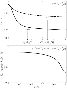
Figure 2: (a) Excess noise ratio for one and two excited neutral modes within the dipole picture $\gamma_{\rm DF}$ (solid line) and the thermal picture $\gamma_{\rm T}$ (dashed line). (b) Excess noise ratio for one and two excited neutral modes within the dipole picture while fixing the edge 1 bias in the asymptotically large regime, $\mu_{1}/\pi k_{B}T_{0}=10$, and varying the edge 2 bias, $\mu_{2}$.

We have taken $\hbar/k_{B}\tau_{c}=0.5$K and $T_{0}=10$mK, which are consistent with Ref. Gross et al., 2012, and we have also taken $\zeta_{1}=\zeta_{2}=\zeta_{3}=\zeta$. A clear signature of noise suppression due to quantum statistics can be seen in Fig. 2(b). Here, the bias for the dipole fermions on edge 1 is fixed at a large value, i.e. $\mu_{1}/\pi k_{B}T_{0}=10\gg 1$, and the bias on edge 2 is varied from $0$ to $\mu_{1}$. We interpret the suppression of noise as $\mu_{2}\rightarrow\mu_{1}$ as due to the reduction in phase space for scattering at the QPC from Pauli blocking. The suppression does not reach strictly zero due to disorder-averaging.

Thermal picture for noise for the random $\nu=2/3$ state: In this case, the backscattering correction to the dc noise reads

$$S_{B}(T_{1},T_{2})=\frac{(e^{*})^{2}}{8\hbar^{2}}\int dt\left[\zeta_{1}^{2}+\zeta_{2}^{2}+4\zeta_{3}^{2}\right]\\ \times F_{g}(T_{1},t)F_{g}(T_{2},t)[1-(2itk_{B}T_{0}/\hbar)],$$ (12)

where $T_{1},T_{2}\geq T_{0}$ are the temperatures of the upper and lower edges at the QPC, which are heated above the base temperature $T_{0}$ via transport of heat by the neutral modes Takei and Rosenow (2011). We define the normalized noise as above, and the excess noise is defined as $S_{\rm ex}(T_{1},T_{2})=S_{B}(T_{1},T_{2})-S_{B}(T_{0},T_{0})$. We consider again two cases: (i) a single thermally-excited neutral mode, i.e. $T_{1}>T_{0}$ and $T_{2}=T_{0}$; and (ii) two thermally-excited neutral modes, i.e. $T_{1}=T_{2}>T_{0}$. The ratio, $\gamma_{\rm T}=S_{\rm ex}(T_{1},T_{1})/S_{\rm ex}(T_{1},T_{0})$, shown as the dashed line in Fig. 2(a), is considerably higher than for the dipole-fermion case.

Comparison to experiment: For $\mu/\pi k_{B}T_{0}\gg 1$ [see solid line in Fig. 2(a)], which may be the regime of relevance for Ref. Gross et al., 2012, we see that the theoretical prediction for $\gamma_{\rm DF}$ falls well below the experimental value $\gamma_{\rm exp}\approx 1.6$. We have checked that this result does not depend on specific values for $\zeta_{i}$. For thermally excited neutral modes [see dashed line in Fig. 2(a)], we see that the experimental value is reproduced when $(T_{1}-T_{0})/T_{0}\approx 0.6$. Ref. Gross et al., 2012 provides lower and upper estimates, $T_{1}=55$mK and $T_{1}=200$-300mK, for the effective temperature at the QPC, putting either of these estimates well above the estimated base temperature of $T_{0}=10$mK. As $(T_{1}-T_{0})/T_{0}\to\infty$ the asymptotic value approaches $\gamma_{\rm T}\approx 1.3$, lower than the asymptotic value $\gamma_{\rm exp}$ found in Gross et al. (2012). However, treating the scaling dimension $g$ of the edge correlation function as a parameter of the theory as in Rosenow and Halperin (2002); Papa and MacDonald (2004), we have reevaluated the noise for $g=1$. In the dipole-fermion picture we find that the theoretical ratio remains well below the experimental value for $\mu/\pi k_{B}T_{0}\gg 1$, while in the thermal picture we now find $\gamma_{\rm T}\approx 1.5$ in the limit of strong thermal bias $(T_{1}-T_{0})/T_{0}\approx 10$, in better agreement with the experiment Gross et al. (2012), and indicating that thermally excited neutral modes are observed there.

In conclusion, we studied the excess charge noise generated by impinging one or two excited neutral modes on a single QPC. We focused on the $\nu=2/3$ FQH state, and considered thermally excited neutral modes as well as biased neutral modes with dipole-fermion excitations. We have found that in the case of two neutral modes impinging on a QPC the noise power reflects the quantum statistics of bosonic thermal excitations vs. dipole-fermions, thus allowing to detect a fingerprint of the quantum statistics of neutral edge excitations.

Acknowledgments $-$ BR acknowledges the DFG for financial support. AS thanks Microsoft Station Q, the US-Israel BSF and the Minerva Foundation for financial support.

References

- Tsui et al. (1982) D. C. Tsui, H. L. Stormer, and A. C. Gossard, Phys. Rev. Lett. 48, 1559 (1982).
- Wen (1991) X. G. Wen, Phys. Rev. B 43, 11025 (1991).
- Kane et al. (1994) C. L. Kane, M. P. A. Fisher, and J. Polchinski, Phys. Rev. Lett. 72, 4129 (1994).
- Levin et al. (2007) M. Levin, B. I. Halperin, and B. Rosenow, Phys. Rev. Lett. 99, 236806 (2007).
- Lee et al. (2007) S.-S. Lee, S. Ryu, C. Nayak, and M. P. A. Fisher, Phys. Rev. Lett. 99, 236807 (2007).
- Kane and Fisher (1995) C. L. Kane and M. P. A. Fisher, Phys. Rev. B 51, 13449 (1995).
- (7) A. Bid, N. Ofek, H. Inoue, M. Heiblum, C. L. Kane, V. Umansky, and D. Mahalu, Nature 466, 585 (2010).
- Dolev et al. (2011) M. Dolev, Y. Gross, R. Sabo, I. Gurman, M. Heiblum, V. Umansky, and D. Mahalu, Phys. Rev. Lett. 107, 036805 (2011).
- Gross et al. (2012) Y. Gross, M. Dolev, M. Heiblum, V. Umansky, and D. Mahalu, Phys. Rev. Lett. 108, 226801 (2012).
- Venkatachalam et al. (2012) V. Venkatachalam, S. Hart, L. Pfeiffer, K. West, and A. Yacoby, ArXiv e-prints (2012), arXiv:1202.6681 [cond-mat.mes-hall] .
- Altimiras et al. (2012) C. Altimiras, H. le Sueur, U. Gennser, A. Anthore, A. Cavanna, D. Mailly, and F. Pierre, Phys. Rev. Lett. 109, 026803 (2012).
- Takei and Rosenow (2011) S. Takei and B. Rosenow, Phys. Rev. B 84, 235316 (2011).
- Rosenow and Halperin (2002) B. Rosenow and B. I. Halperin, Phys. Rev. Lett. 88, 096404 (2002).
- Papa and MacDonald (2004) E. Papa and A. H. MacDonald, Phys. Rev. Lett. 93, 126801 (2004).