Evaluations of low-energy physical quantities in QCD with IR freezing of the coupling

Abstract

The ${\overline{\rm MS}}$-like schemes in QCD have in general the running coupling which contains Landau singularities, i.e., singularities outside the timelike semi-axis, at low squared momenta. As a consequence, evaluation of the spacelike quantities, such as current correlators, in terms of (powers of) such a coupling then results in quantities which contradict the basic principles of Quantum Field Theories. On the other hand, in those QCD frameworks where the running coupling remains finite at low squared momenta (IR freezing), the coupling usually does not have Landau singularities in the complex plane of the squared momenta. I argue that in such QCD frameworks the spacelike quantities should not be evaluated as a power series, but rather as a series in derivatives of the coupling with respect to the logarithm of the squared momenta. Such series show considerably better convergence properties. Moreover, Padé-related resummations of such logarithmic derivative series give convergent series, thus eliminating the practical problem of series divergence due to renormalons.

1 Introduction

One of the main challenges of the contemporary particle physics is to understand and adequately describe QCD at low scales $\stackrel{{\scriptstyle<}}{{\sim}}1$ GeV. The usual perturbative (pQCD) approach in $\overline{\rm MS}$-like schemes leads to the running coupling $a(Q^{2})$ ($\equiv\alpha_{s}^{\rm(pt)}(Q^{2})/\pi$) which has singularities in the regime outside the negative axis in the complex $Q^{2}$-plane (where $q^{2}\equiv-Q^{2}$ is the usual squared momentum transfer). Such singularities are not present in the spacelike renormalization scale invariant quantities $d(Q^{2})$, as a consequence of the basic principles of quantum field theories [1] such as locality, unitarity and microcausality. If such quantities are to be evaluated as functions of the running coupling $a(\kappa Q^{2})$ (with $\kappa\sim 1$), then the coupling $a$ should not have such (Landau) singularities. Thus $a(Q^{2})$ should be an analytic (holomorphic) function of $Q^{2}$ in the entire complex plane, with the exception of the negative semiaxis $Q^{2}<-M^{2}_{\rm thr}$ (where $M^{2}_{\rm thr}\sim 10^{-1}\ {\rm GeV}^{2}$).

Such a behavior of $a(Q^{2})$ is indirectly supported by calculations using functional methods [2; 3; 4; 5; 6; 7; 8; 9] and lattice calculations [10; 11; 12; 13]. Most of these works suggest that the running coupling has a finite limit when $Q^{2}\to 0$, i.e., IR freezing (IR fixed point). IR freezing is obtained also in models with AdS/CFT correspondence modified by a dilaton backgound [14; 15].

In the works [16; 17; 18; 19; 20; 21; 22; 23; 24; 25; 26; 27] the mentioned type of analyticity was imposed on the QCD coupling $a(Q^{2})$, within various scenarios, and as a result the obtained holomorphic coupling turned out to be IR finite (for reviews, see [28; 29]). Infrared finiteness of the coupling and its analyticity, however, do not necessarily always go together. For example, a model with holomorphic coupling which is infinite in the limit $Q^{2}\to 0$ was constructed and used in Refs. [30; 31]. The opposite example is that of Ref. [32] where the coupling is finite in the limit $Q^{2}\to 0$ but has (Landau) singularities within the complex $Q^{2}$ plane outside the real axis (see the comments about this coupling in Ref. [33]).

Yet another question is whether a purely perturbative coupling $a(Q^{2})$, in the $\overline{\rm MS}$-like schemes, can have a holomorphic (and IR finite) coupling $a(Q^{2})$ [$\overline{\rm MS}$-like schemes are speficied later on in the comments after Eq. (1)]. In Ref. [33] it was shown that such schemes are difficult to obtain, and appear to lead to sudden jumps in the values of the coefficients $\beta_{j}$ of the beta function when $j$ increases. Yet there exist QCD models with holomorphic and IR finite coupling $a(Q^{2})$ which practically merge with the underlying pQCD couplings $a_{\rm pt}(Q^{2})$ in the $\overline{\rm MS}$-like schemes at higher $|Q^{2}|$, i.e., $a(Q^{2})-a_{\rm pt}(Q^{2})\sim(Q^{2}/\Lambda^{2})^{N}$ at $Q^{2}>\Lambda^{2}$ (where $\Lambda^{2}\sim 10^{-1}\ {\rm GeV}^{2}$) with $N=4,5$, Refs. [34; 25; 26; 27]. In particular, the analytic model [27] has $N=5$, and reproduces the experimental value of the $\tau$ lepton semihadronic (strangeless) decay ratio $r_{\tau}$, the latter quantity being one of the few well measured low-momenta QCD quantities at present.

Here I will present three frameworks with IR finite coupling $a(Q^{2})$ which, in addition, is holomorphic in the $Q^{2}$ complex plane (with the exception of a semiaxis $Q^{2}<-M^{2}_{\rm thr}$). I will argue that the renormalization scale invariant spacelike quantities (such as spacelike observables) $d(Q^{2})$ at low $|Q^{2}|\sim 1\ {\rm GeV}^{2}$ should not be evaluated, as usually assumed, as a series in powers $a(\kappa Q^{2})^{n+1}$, but rather as a series in logarithmic derivatives ${\widetilde{a}}_{n+1}(\kappa Q^{2})\propto(\partial/\partial\ln Q^{2})^{n}a(\kappa Q^{2})$. This, because the renormalization scale dependence of the (truncated) power series grows out of control and the series shows strong divergence (compounded by the renormalon problem) when the number of terms increases. Further, I consider a resummation method of Refs. [35; 36; 37; 38], which is based on the mentioned truncated series in logarithmic derivatives and is a generalization of the diagonal Padé method. I show that this generalized Padé method in the frameworks with IR finite coupling gives results which are renormalization scale invariant and converge very well when the number of terms in the initial truncated series increases. Numerical evidence is presented for the large-$\beta_{0}$ Adler function, which is a spacelike renormalization scale invariant quantity whose expansion is known to all orders. Finally, I argue that the obtained conclusions are applicable also to the timelike observables, because they can be represented as integral transformations of the aforementioned spacelike quantities. A more detailed consideration of these topics has been presented in Ref. [39].

2 Three scenarios with IR finite (and holomorphic) coupling

To fix the notations, I start here with the (truncated) perturbative RGE

$$\frac{\partial a_{\rm pt}(Q^{2};{\beta_{2}},\ldots)}{\partial\ln Q^{2}} = -\sum_{j=0}^{n-1}\beta_{j}\>a_{\rm pt}(Q^{2};{\beta_{2}},\ldots)^{j+2}=-\beta_{0}a_{\rm pt}^{2}(1+c_{1}a_{\rm pt}+c_{2}a_{\rm pt}^{2}+\ldots)\ ,$$ (1)

where $a_{\rm pt}\equiv\alpha_{s}/\pi=g_{s}/(4\pi^{2})$, the first two beta coefficients are universal [$\beta_{0}=(1/4)(11-2N_{f}/3)$, $\beta_{1}=(1/16)(102-38N_{f}/3)$], and the other coefficients $\beta_{k}\equiv c_{j}\beta_{0}$ ($k\geq 2$) characterize the perturbative renormalization scheme. The renormalization schemes are called $\overline{\rm MS}$-like if the coefficients $\beta_{j}$ depend on the (quark) mass via the number of effective quark flavors $N_{f}$ and are polynomials of $N_{f}$ of order $j$ for $j\geq 2$. For the $\Lambda$-scale convention ($\Lambda$ “scheme”) I take $\Lambda_{\overline{\rm MS}}$.

2.1 Coupling with dynamical gluon mass

A representative case of QCD coupling $a(Q^{2})$ with finite $Q^{2}\to 0$ limit is the case with effective (dynamical) gluon mass $m$, Refs. [40; 41; 42; 43]

$$a^{(m)}(Q^{2})=a_{\rm pt}(Q^{2}+m^{2})\ ,$$ (2)

where I take $m=0.8$ GeV, $N_{f}=3$, and $a_{\rm pt}$ as the usual pQCD coupling in the $c_{2}=c_{3}=\ldots=0$ renormalization scheme which allows exact solution in terms of the Lambert function, Refs. [44; 45] (see also Ref. [46])

$$a_{\rm pt}(\kappa Q^{2})=-\frac{1}{c_{1}}\frac{1}{\left[1+W_{\mp 1}(z)\right]}\ .$$ (3)

Here, $Q^{2}=|Q^{2}|\exp(i\phi)$; $W_{-1}$ and $W_{+1}$ are the branches of the Lambert function for $0\leq\phi<+\pi$ and $-\pi<\phi<0$, respectively, and $z$ is defined as

$$z=-\frac{1}{c_{1}e}\left(\frac{\kappa|Q^{2}|}{\Lambda_{\rm L.}^{2}}\right)^{-\beta_{0}/c_{1}}\exp\left(-i{\beta_{0}}\phi/c_{1}\right)\ ,$$ (4)

where $\Lambda_{\rm L.}$ is the Lambert QCD scale. At $N_{f}=3$ we have $\Lambda_{\rm L.}=\Lambda_{\overline{\rm MS}}/0.72882$. I use $\Lambda_{\rm L.}=0.487$ GeV, thus $\Lambda_{\overline{\rm MS}}=0.355$ GeV. This gives at $\mu^{2}=m_{\tau}^{2}$ the value $a^{(m)}(m_{\tau}^{2})=0.293/\pi$.

2.2 (Fractional) Analytic Perturbation Theory (F)APT

This is the model developed in [16; 17; 18; 19; 20; 21; 22; 23; 24]. The analogs $a^{\rm(FAPT)}_{\nu}(Q^{2})$ of the power $a_{\rm pt}(Q^{2})^{\nu}$ (where $\nu$ can be noninteger; and $a_{\rm pt}$ is in a $\overline{\rm MS}$-like renormalization scheme) are obtained by “minimally” analytizing the pQCD expression $a_{\rm pt}(Q^{2})^{\nu}$. This means that the cuts of $a_{\rm pt}(Q^{2})^{\nu}$ on the negative axis $Q^{2}\equiv-\sigma<0$ are kept unchanged, but the Landau singularities (cuts and poles) on the positive $Q^{2}$ axis are eliminated. This leads via Cauchy theorem to the following dispersive expression for $a_{\nu}$:

$$a^{\rm{(FAPT)}}_{\nu}(Q^{2})=\frac{1}{\pi}\int_{\sigma=0}^{\infty}\frac{d\sigma{\rho^{\rm{(pt)}}_{\nu}}(\sigma)}{(\sigma+Q^{2})}\qquad\left[\not=a^{\rm{(FAPT)}}(Q^{2})^{\nu}\right]\ ,$$ (5)

where ${\rho^{\rm{(pt)}}_{\nu}}(\sigma)={\rm Im}a_{\rm pt}(-\sigma-i\epsilon)^{\nu}$ is the discontinuity function on the cut. At one-loop level $a_{\nu}^{\rm(FAPT)}$ has an explicit expression and was constructed and used in Ref. [22]

$$a_{\nu}(Q^{2})^{\rm(FAPT,1-\ell.)}=\frac{1}{\beta_{0}^{\nu}}\left(\frac{1}{\ln^{\nu}(z)}-\frac{{\rm Li}_{-\nu+1}(1/z)}{\Gamma(\nu)}\right)\ ,$$ (6)

where $z\equiv Q^{2}/\Lambda^{2}$ and ${\rm Li}_{-\nu+1}(z)$ is the polylogarithm function of order $-\nu+1$. FAPT expressions for higher loops can be obtained via expansions of the one-loop result [23; 24]. A review of FAPT is given in Refs. [28; 29]. Mathematical packages for numerical calculation are given in Refs. [47; 48; 49]. I will use for the underlying renormalizations scheme $c_{2}=c_{3}=\cdots=0$, and for the number of active quark flavors $N_{f}=3$. The (F)APT scale is fixed at ${\Lambda}_{\rm L.}({\rm(F)APT})=0.572$ GeV, giving the value $a^{\rm(FAPT)}(m_{\tau}^{2})=0.295/\pi$.

2.3 Analytic model with two deltas (2$\delta$anQCD)

This model also has holomorphic $a(Q^{2})$, and is based on the general dispersive relation for such couplings,

$$a(Q^{2})=\frac{1}{\pi}\int_{\sigma=0}^{\infty}\frac{d\sigma{\rho}(\sigma)}{(\sigma+Q^{2})}\ ,$$ (7)

where ${\rho}$ is the discontinuity function of $a$: ${\rho}(\sigma)={\rm Im}a(-\sigma-i\epsilon)$. In Ref. [27] this discontinuity function was approximated at high scales $\sigma\geq M_{0}^{2}$ (${\sim}1\ {\rm GeV}^{2}$) by its pQCD analog $\rho^{\rm(pt)}(\sigma)={\rm Im}a_{\rm pt}(-\sigma-i\epsilon)$. In the unknown low-scale regime, $0<\sigma<M_{0}^{2}$ it was approximated by two delta functions

$$\rho(\sigma)^{(2\delta)}(\sigma) = \pi F_{1}^{2}\delta(\sigma-M_{1}^{2})+\pi F_{2}^{2}\delta(\sigma-M_{2}^{2})+\Theta(\sigma-M_{0}^{2})\rho^{\rm(pt)}(\sigma)\ .$$ (8)

This gives via the dispersion relation (7) the following coupling:

$$a^{(2\delta)}(Q^{2}) = \frac{F_{1}^{2}}{Q^{2}+M_{1}^{2}}+\frac{F_{2}^{2}}{Q^{2}+M_{2}^{2}}+\frac{1}{\pi}\int_{M_{0}^{2}}^{\infty}d\sigma\;\frac{\rho^{\rm(pt)}(\sigma)}{(Q^{2}+\sigma)}\ .$$ (9)

The parameters $F_{j}$ and $M_{j}$ ($j=1,2$) appearing in the delta functions, and the pQCD-onset scale $M_{0}$, were adjusted so that the correct value of the semihadronic tau decay ratio $r_{\tau}\approx 0.20$ ($V+A$ channel) was reproduced and that the difference from the underlying pQCD coupling at high $|Q^{2}|>\Lambda^{2}$ is as strongly suppressed as possible

$$a^{(2\delta)}(Q^{2})-a_{\rm pt}(Q^{2}) \sim (\Lambda^{2}/Q^{2})^{5}\ .$$ (10)

The renormalization scheme parameter value $c_{2}=-4.76$ of the underlying $N_{f}=3$ coupling $a_{\rm pt}$ was chosen in such a way that $M_{0}$ and the value of $a^{(2\delta)}(Q^{2}=0)$ were reasonable, i.e., not too high: $M_{0}=1.25$ GeV and $a(0)\approx 0.78$ ($c_{2}$ can be varied between $-5.7$ and $-2.1$, see Table I in Ref. [50]). In addition, it was convenient to choose $c_{j}=c_{2}^{j-1}/c_{1}^{j-2}$ ($j=3,4,\ldots$), because then the exact solution of the underlying pQCD coupling is also known in terms of the Lambert function (Refs. [44; 21], cf. also Ref. [51]). I refer for more details on the model to Ref. [27]. The input values of the model are the central ones used in Ref. [27] (among them: $c_{2}=-4.76$, $\Lambda_{\rm L.}=0.260$ GeV) and give the value $a^{\rm(2\delta)}(m_{\tau}^{2})=0.291/\pi$.

3 Series in powers and logarithmic derivatives

A spacelike QCD quantity $d(Q^{2})$ with renormalization scale invariance, such as the derivative of a current correlator, is usually evaluated in $\overline{\rm MS}$-like schemes as a truncated power series

$$d(Q^{2};\kappa)_{\rm pt}^{[N]}=a_{\rm pt}(\kappa Q^{2})+\sum_{j=1}^{N-1}d_{j}(\kappa)\;a_{\rm pt}(\kappa Q^{2})^{j+1}\ ,$$ (11)

where $\mu^{2}\equiv\kappa Q^{2}$ is the renormalization scale ($\kappa\sim 1$), and usually $N=3$ or $N=4$. Due to truncation, there appears the dependence on the renormalization scale parameter $\kappa$

$$\frac{\partial d_{\rm pt}^{[N]}}{\partial\ln\kappa}=K_{N}a_{\rm pt}(\kappa Q^{2})^{N+1}+K_{N+1}a_{\rm pt}(\kappa Q^{2})^{N+2}+\cdots\;\sim a^{N+1}\ .$$ (12)

This dependence may be quite large at low $Q^{2}$ and large $N$, one reason being the increase of the coefficients $K_{N+k}$ ($\sim d_{N+k-1}$) when $N+k$ increases (due to renormalon growth); the other reason is the increase of $a_{\rm pt}(\kappa Q^{2})^{N+k+1}$ when $N+k$ increases because $a_{\rm pt}(\kappa Q^{2})$ is large due to vicinity of the Landau singularities (at low positive $Q^{2}$). These two reasons also result in a very strongly divergent behavior of the truncated power series (11) when the number of terms $N$ increases and $|Q|$ is low.

However, the power series can be reorganized in a series of logarithmic derivatives [52; 53; 33]

$${{\widetilde{a}}}_{{\rm pt},n}(Q^{2})\equiv\frac{(-1)^{n-1}}{\beta_{0}^{n-1}(n-1)!}\left(\frac{\partial}{\partial\ln Q^{2}}\right)^{n-1}a_{\rm pt}(Q^{2})\ ,\qquad(n=1,2,\ldots)\ .$$ (13)

It can be shown by the RGE (1) that

$${{\widetilde{a}}}_{{\rm pt},n}(Q^{2})=a_{\rm pt}(Q^{2})^{n}+\sum_{m\geq 1}k_{m}(n)a_{\rm pt}(Q^{2})^{n+m}\ ,$$ (14)

where $k_{m}(n)$ depend on the coefficients $c_{j}$ of the RGE (1). These relations can be inverted

$${a}_{{\rm pt}}(Q^{2})^{n}={{\widetilde{a}}}_{{\rm pt},n}(Q^{2})+\sum_{m\geq 1}{{\widetilde{k}}}_{m}(n){{\widetilde{a}}}_{{\rm pt},n+m}(Q^{2})\ .$$ (15)

Inserting these expressions in the truncated power series (11) results in the reorganized truncated series (mpt) in the logarithmic derivatives

$$d(Q^{2};\kappa)_{\rm mpt}^{[N]}=a_{\rm pt}(\kappa Q^{2})+\sum_{j=1}^{N-1}{\widetilde{d}}_{j}(\kappa)\;{\widetilde{a}}_{{\rm pt},j+1}(\kappa Q^{2})\ .$$ (16)

The two series (11) and (16) differ in terms $\sim a_{\rm pt}^{N+1}\sim{\widetilde{a}}_{{\rm pt},N+1}$ due to truncation. Further, the renormalization scale dependence has now a different, more simple, expression than in the case of the truncated power series (12)

$$\frac{\partial d_{\rm mpt}^{[N]}}{\partial\ln\kappa}=-\beta_{0}N{\widetilde{d}}_{N-1}(\kappa){\widetilde{a}}_{{\rm pt},N+1}(\kappa Q^{2})\ .$$ (17)

In pQCD with $\overline{\rm MS}$-like scheme, the two approaches of evaluation give comparable results, even at low $|Q|$, as demonstrated in Ref. [54]. However, in QCD with coupling $a(Q^{2})$ finite in the IR regime, at low $|Q|$ the method (16) with logarithmic derivatives is significantly better than (11) and, in fact, is the correct one, as argued in Refs. [52; 53] and further applied in Refs. [26; 27; 38; 50]. This has to do with the fact that beta function $\beta(a)$ of such IR finite holomorphic coupling $a(Q^{2})$ is not fully represented by the power expansion (1), but contains at low $|Q|$ significant nonperturbative contributions, i.e., contributions nonanalytic in $a$ such as $\exp(-K/a(Q^{2}))\sim(\Lambda^{2}/Q^{2})^{K/\beta_{0}}$. The same is true for the derivative on the left-hand side of Eq. (12) when $a_{\rm pt}\mapsto a$. The equality (12) is not valid when we have $a$ (instead of $a_{\rm pt}$) in the theory, the difference between the left-hand and the right-hand side being a nonperturbative contribution (invisible to powers of $a$) which tends to get out of control when $N$ is large. Hence, additional terms enter the renormalization scale dependence of the truncated power series in such frameworks and make it even more out of control at larger $N$. On the other hand, it can be shown that the scale dependence for the reorganized series (mpt) in such frameworks ($a_{\rm pt}\mapsto a$ and ${\widetilde{a}}_{\rm pt,n}\mapsto{\widetilde{a}}_{n}$) keeps the simple form (17), i.e., this equality remains exact in such frameworks. The right-hand side of Eq. (17) (with $a_{\rm pt}\mapsto a$) contains the nonperturbative contributions - they are contained in the single term there, the logarithmic derivative ${\widetilde{a}}_{N+1}(\kappa Q^{2})$ which, in contrast to powers $a(\kappa Q^{2})^{N+k}$, “sees” such contributions.

This means that in QCD with the coupling $a(Q^{2})$ finite at $Q^{2}\to 0$ we should not use as the basis for the evaluations the power series, but the reorganized series (man: for “modified analytic”)

$$d(Q^{2};\kappa)_{\rm man}^{[N]}=a(\kappa Q^{2})+\sum_{j=1}^{N-1}{\widetilde{d}}_{j}(\kappa)\;{\widetilde{a}}_{j+1}(\kappa Q^{2})\ ,$$ (18)

where

$${{\widetilde{a}}}_{n}(Q^{2})\equiv\frac{(-1)^{n-1}}{\beta_{0}^{n-1}(n-1)!}\left(\frac{\partial}{\partial\ln Q^{2}}\right)^{n-1}a(Q^{2})\ ,\qquad(n=1,2,\ldots)\ .$$ (19)

An additional reason for the better convergence and the weaker renormalization scale dependence of such series at low $|Q|$ is the empirical fact that in virtually all models with holomorphic IR finite coupling $a(Q^{2})$ we have the hierarchy $|a(Q^{2})|>|{\widetilde{a}}_{2}(Q^{2})|>|{\widetilde{a}}_{3}(Q^{2})|>\cdots$ for any $Q^{2}$ (and not just when $|Q^{2}|$ is large).

The approach described here was extended in Ref. [55], in the frameworks with IR finite holomorphic $a(Q^{2})$, to the evaluation of quantities whose perturbative power expansion (11) involves noninteger powers of $a_{\rm pt}$.

It is interesting that in the (F)APT model the evaluation with the analogs $a^{\rm{(FAPT)}}_{n}(Q^{2})$ of the powers of $a_{\rm pt}^{n}$, Eqs. (5)-(6), is equivalent to the approach described here, because it turns out that for (F)APT model the relations (15) are fulfilled

$$a^{\rm{(FAPT)}}_{n}(Q^{2})={{\widetilde{a}}}^{\rm{(FAPT)}}_{{\rm pt},n}(Q^{2})+\sum_{m\geq 1}{{\widetilde{k}}}_{m}(n){{\widetilde{a}}}^{\rm{(FAPT)}}_{n+m}(Q^{2})\ ,$$ (20)

and this even when $n$ is noninteger ($n=\nu$), as argued in Ref. [55] (see also Ref. [21], for integer $n$). Nonetheless, the approach reviewed here can be applied to general models with holomorphic coupling $a(Q^{2})$ with IR finite value, while the approach Eq. (5) only within the (F)APT.

4 Numerical evidence

I will illustrate numerically the effects of various evaluations in the case of the Adler function in the large-$\beta_{0}$ approximation. The effective charge of the (massless) Adler function is defined as

$$d_{\rm Adl}(Q^{2})=-(2\pi^{2})\frac{d\Pi(Q^{2})}{d\ln Q^{2}}-1\ ,$$ (21)

where $\Pi(Q^{2})$ is the correlator of the nonstrange charged hadronic currents (vector or axial) in the massless limit. The perturbation expansion of $d_{\rm Adl}$ in powers of $a_{\rm pt}$ has the form (11); however, only the first four coefficients are fully known at the moment ($d_{0}=1$; $d_{j}$ with $j=1,2,3$). I want to test, however, the renormalization scale dependence and the convergence of the evaluations based on the truncated perturbation series of the type (11) and (16) [(18)], in pQCD and in the mentioned IR finite coupling scenarios, when the truncation number $N$ is increasing. The coefficients $d_{n}$ and ${\widetilde{d}}_{n}$ in $\overline{\rm MS}$-type schemes can be written as polynomials of $N_{f}$ of order $n$, and thus also as polynomials in powers of $\beta_{0}$ of order $n$

$${\widetilde{d}}_{n}(\kappa)=c_{n,n}(\kappa)\beta_{0}^{n}+c_{n,n-1}\beta_{0}^{n-1}+\ldots+c_{n,0}\ ,$$ (22)

The leading-$\beta_{0}$ (LB) part of these coefficients, ${\widetilde{d}}_{n}^{\rm(LB)}=c_{n,n}\beta_{0}^{n}$, are known to all orders [56; 57]. This LB quantity can then be written formally as an integral over momenta $tQ^{2}$ [58]

$$d_{\rm Adl}^{\rm(LB)}(Q^{2})_{\rm(m)pt} = \int_{0}^{\infty}\frac{dt}{t}\;F_{d}(t)a_{\rm pt}(tQ^{2}e^{{\cal C}})$$ (23)

$$= a_{\rm pt}(\kappa Q^{2})+{\widetilde{d}}_{1}^{\rm(LB)}(\kappa){{\widetilde{a}}}_{{\rm pt},2}(\kappa Q^{2})+\cdots+{\widetilde{d}}_{n}^{\rm(LB)}(\kappa){{\widetilde{a}}}_{{\rm pt},n+1}(\kappa Q^{2})+\cdots$$ (24)

$$= a_{\rm pt}(\kappa Q^{2})+d_{1}^{\rm(LB)}(\kappa)a_{\rm pt}(\kappa Q^{2})^{2}+\cdots d_{n}^{\rm(LB)}(\kappa)a_{\rm pt}(\kappa Q^{2})^{n+1}+\cdots\ ,$$ (25)

where $F_{d}(t)=t{\hat{w}}_{d}(t)/4$ is the distribution function of the LB Adler function obtained in Ref. [58], and ${\cal C}=-5/3$ in the $\Lambda_{\bar{M}S}$-convention. It is important to point out that the coupling $a_{\rm pt}$ in the integral (23) can run according to $N$-loop RGE ($N\geq 1$), not just one-loop. The quantity defined in this way is renormalization scale ($\kappa$) independent, although it acquires renormalization scheme dependence when $a_{\rm pt}$ runs according to the $N$-loop RGE with $N\geq 3$ (dependence on the scheme parameters $c_{2},\ldots,c_{N-1}$). Nonetheless, I will use this quantity for testing the quality of different evaluations, i.e., evaluations based on the truncated series (24)-(25). The expansion (24) is obtained from the integral representation (23) by Taylor-expanding the coupling $a_{\rm pt}(tQ^{2}e^{{\cal C}})$ around the point $\ln\mu^{2}\equiv\ln\kappa Q^{2}$ and exchanging the order of integration and summation, and using the relations

$${{\widetilde{d}}}_{n}^{\rm(LB)}(\kappa) \equiv \beta_{0}^{n}c_{n,n}(\kappa)=(\beta_{0})^{n}(-1)^{n}\int_{t=0}^{\infty}d(\ln t)\ln^{n}\left(t\kappa^{-1}e^{{\cal C}}\right)F_{d}(t)\ ,$$ (26)

$$c_{n,n}(\kappa) = c_{n,n}(e^{\cal C})+\sum_{k=1}^{n}\left(\begin{array}[]{c}n\\ k\end{array}\right)\ln^{k}\left(\kappa e^{-{\cal C}}\right)c_{n-k,n-k}(e^{\cal C})\ ,$$ (29)

where

$$c_{n,n}(e^{\cal C})=\frac{3}{4}C_{F}\left(\frac{d}{db}\right)^{n}P(1-b)|_{b=0}$$ (30)

with $C_{f}=4/3$ and $P(x)$ is the trigamma function obtained in Ref. [56]

$$P(x)=\frac{32}{3(1+x)}\sum_{k=1}^{\infty}\frac{(-1)^{k}k}{(k^{2}-x^{2})^{2}}\ .$$ (31)

While ${{\widetilde{d}}}_{n}^{\rm(LB)}$ are the complete LB parts of the full coefficients ${{\widetilde{d}}}_{n}$, the coefficients $d_{n}^{\rm(LB)}$ in the power series (25) contain in general also beyond-the-leading-$\beta_{0}$ terms. Only in the case of one-loop RGE running the equality holds: $d_{n}^{\rm(LB)}={{\widetilde{d}}}_{n}^{\rm(LB)}$.

In $\overline{\rm MS}$-type schemes in pQCD the running coupling $a_{\rm pt}(tQ^{2}e^{{\cal C}})$ in the integral (23) has Landau singularities at low $t$, therefore the integral becomes ambiguous and an integration prescription must be imposed – usually the (generalized) principal value which I will adopt here, in order to define the “exact” LB value in pQCD. On the other hand, in QCD with finite $a(Q^{2})$ in the infrared, all the formulas (23)-(25) are repeated, with the simple replacements

$$a_{\rm pt}\mapsto a\ ,\qquad{\widetilde{a}}_{{\rm pt},n}\mapsto{\widetilde{a}}_{n}\ .$$ (32)

Moreover, the exact LB value, i.e., the integral (23), now becomes finite and unambiguous, due to the absence of the Landau singularities.

The numerical evaluations will be based on the truncated series (24) and (25), for pQCD in the $c_{2}=c_{3}=\cdots=0$ renormalization scheme; and on these truncated series with the replacements (32) for the three frameworks described in Sec. 2.

4.1 Stability under the variation of the renormalization scale

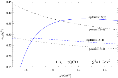
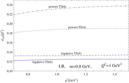
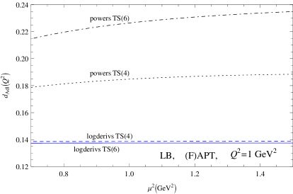
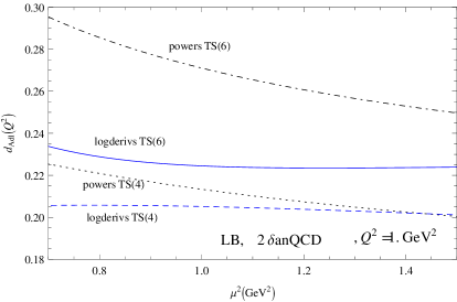
Figure 1: The LB Adler function $d_{\rm Adl}^{\rm(LB)}(Q^{2})$, at leading-$\beta_{0}$ (LB), for $Q^{2}=1\ {\rm GeV}^{2}$, as a function of the (squared) spacelike renormalization scale $\mu^{2}$: (a) in pQCD (the upper left-hand Figure); and in the three frameworks with the coupling $a(Q^{2})$ finite in the IR: (b) the model of Sec. 2.1 with effective constant gluon mass (the upper right-hand Figure); (c) (F)APT model of Sec. 2.2 (the lower left-hand Figure); (d) 2$\delta$ analytic QCD model of Sec. 2.3 (the lower right-hand Figure). The truncatetions are made at $\sim a^{4}$ (${\widetilde{a}}_{4}$) and $\sim a^{6}$ (${\widetilde{a}}_{6}$).

The results of the LB Adler function, Eqs. (24)-(25) truncated at order $N=4$ and $N=6$, for $Q^{2}=1\ {\rm GeV}^{2}$, are presented as functions of the squared (spacelike) renormalization scale $\mu^{2}=\kappa Q^{2}$ in Figs. 1 for the pQCD case and for the three models with IR finite $a(Q^{2})$ described in Sec. 2. We can see that the truncated series in the logarithmic derivatives show greater stability under the variation of $\mu^{2}$ in the three QCD frameworks with IR finite coupling.

4.2 Convergence properties of various evaluations

Here I will compare the convergence (divergence) behavior of the evaluations of truncated series (24)-(25) in pQCD and the three models of Sec. 2. I will add here yet another evaluation method, based on the truncated series (24). This method was constructed in Refs. [35; 36] in the context of pQCD, and was applied with success to QCD frameworks with IR finite holomorphic $a(Q^{2})$ in Refs. [37; 38]. It is an approximation constructed on the basis of the truncated series in logarithmic derivatives, truncated at order ${\widetilde{a}}_{2M}$ ($M=1,2,3,\cdots$), and can be written in the following form:

$${\cal G}^{[M/M]}_{d}(Q^{2})=\sum_{j=1}^{M}{\widetilde{\alpha}}_{j}\;a(\kappa_{j}Q^{2})\ .$$ (33)

The scale parameters $\kappa_{j}$ and the coefficients ${\widetilde{\alpha}}_{j}$ (where: ${\widetilde{\alpha}}_{1}+\ldots+{\widetilde{\alpha}}_{M}=1$) are determined uniquely from the coefficients ${\widetilde{d}}_{j}$ ($j=1,\cdots,2M-1$). I refer for details of the construction of this expression to the mentioned literature. Several aspects can be pointed out: (a) the approximant (33) can be regarded as a (nontrivial) generalization of the diagonal Padé (dPA) method [59], the latter giving renormalization scale independent results at the one-loop level; (b) the running of $a$ can be to any loop order (not just one-loop), and the result (33) is exactly independent of the renormalization scale used in the original series of logarithmic derivatives; (c) the approximant fulfills the basic requirement of the approximant of order $N=2M$, Ref. [37]

$$d(Q^{2})-{\cal G}^{[M/M]}_{d}(Q^{2})={\cal O}({\widetilde{a}}_{2M+1})\qquad\left[={\cal O}(a^{2M+1})\right]\ .$$ (34)

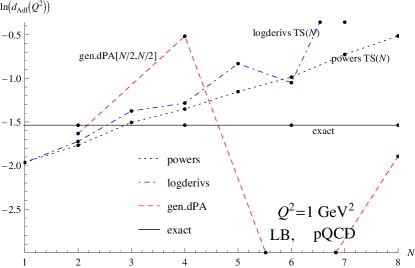
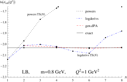
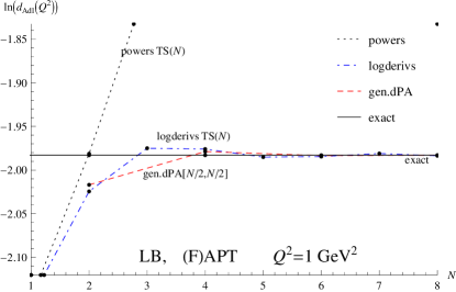
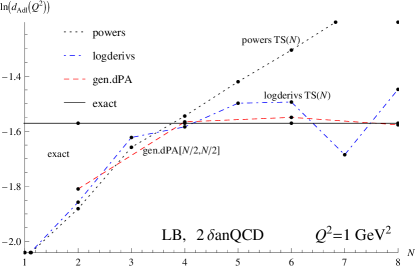
Figure 2: The behavior of the LB Adler function effective charge $d_{\rm Adl}^{\rm(LB)}(Q^{2}=1{\rm GeV}^{2})$ as a function of the truncation order $N$ [the vertical axis represents $\ln d_{\rm Adl}^{\rm(LB)}(Q^{2})$]: (a) pQCD (upper left); (b) the model with constant effective gluon mass of Sec. 2 (upper right); (c) (F)APT model of Sec. 2.2 (lower left); (d) 2$\delta$ analytic QCD model of Sec. 2.3 (lower right).

I performed the direct evaluations of the truncated power series (25) and the series in logarithmic derivatives (24), as well as the evaluation (33) [based on the truncated series (24)] for various orders of truncation $N$, at the chosen renormalization scale $\mu^{2}=Q^{2}$ ($\kappa=1$), in order to see the behavior of these series with increasing $N$ and to compare the results with the “exact” result (23) [with $a_{\rm pt}\mapsto a$ there]. The results are given in Figs. 2, for pQCD (in $c_{2}=c_{3}=\cdots=0$ scheme) and for the three QCD frameworks of Sec. 2, at $Q^{2}=1\ {\rm GeV}^{2}$. We can see the following: in all three IR finite frameworks, (a) the naive power series gives highly divergent behavior; (b) the series in logarithmic derivatives stabilizes to a degree at intermediate orders $N\approx 3$-$6$ and then starts to oscillate increasingly when $N$ increases further; (c) the dPA-related method of Eq. (33) gives results which converge to the exact LB value (23) [cf. also Eq. (32)] surprisingly well as $N$ increases, there is no trace of possible divergent behavior at high $N$ (I checked this up to $N=20$). On the other hand, for the ($\overline{\rm MS}$-like) pQCD, all three methods give consistently divergent behavior with increasing $N$, this being mainly the consequence of the vicinity of the Landau singularities when $Q^{2}\sim 1\ {\rm GeV}^{2}$. One reason for the failure of the power series (in all cases) and of the series in logarithmic derivatives (in pQCD already at low $N$; in IR finite framework at high $N>10$) is the renormalon growth of the coefficients $c_{n,n}\sim n!$. The dPA-related method (33), on the other hand, appears to deal with the renormalon growth of the coefficients very well, and the only problem for that method are the Landau singularities which, in the frameworks with holomorphic (analytic) and IR finite $a(Q^{2})$ are nonexistent. Even more, this dPA-related method, which is based on the truncated series in logarithmic derivatives, is completely renormalization scale independent, i.e., in Figs. 1 it would be represented by exactly horizontal lines.

5 Timelike observables

The timelike observables ${\cal T}(\sigma)$, such as cross sections and decay widths, can be related with spacelike observables ${\cal F}(Q^{2})$, via integral transformations.

Often the integral transformations between ${\cal T}(\sigma)$ and ${\cal F}(Q^{2})$ are the same or similar as between the $(e^{+}e^{-}\to\ {\rm hadrons})$ ratio ${\cal T}(\sigma)=R(\sigma)$ and the Adler function ${\cal F}(Q^{2})=d_{\rm Adl}(Q^{2})$

$${\cal F}(Q^{2})=Q^{2}\int_{0}^{\infty}\frac{d\sigma\ {\cal T}(\sigma)}{(\sigma+Q^{2})^{2}}\ ,\qquad{\cal T}(\sigma)=\frac{1}{2\pi i}\int_{-\sigma-i\varepsilon}^{-\sigma+i\varepsilon}\frac{dQ^{{}^{\prime}2}}{Q^{{}^{\prime}2}}{\cal F}(Q^{{}^{\prime}2})\ ,$$ (35)

where in the last integral the integration contour is in the complex $Q^{{}^{\prime}2}$-plane encircling the singularities of the integrand; for example, on the circle of radius $\sigma$ in the counterclockwise direction (and not cutting the negavive semiaxis).

The basic idea for evaluations of such timelike quantities in the QCD frameworks with analytic and IR finite $a(Q^{2})$ is that first the spacelike quantity ${\cal F}(Q^{{}^{\prime}2})$ is evaluated (with $Q^{{}^{\prime}2}$ on the mentioned circle), with aforementioned method of truncated series in logarithmic derivatives, or the dPA-related method (33); then the contour integral (35) is applied on this quantity.

6 Summary

Theoretical approaches such as Dyson-Schwinger equations and other functional methods, most of the analytic (holomorphic) QCD models, as well as lattice calculations, suggest that the QCD running coupling $a(Q^{2})$ ($\equiv\alpha_{s}(Q^{2})/\pi$) is finite in the IR limit $Q^{2}\to 0$. Here, it was argued that in such frameworks the evaluation of the renormalization scale invariant spacelike QCD quantities $d(Q^{2})$, at low $|Q^{2}|\sim 1\ {\rm GeV}^{2}$, should not be performed as a naive truncated power series, but rather as a truncated series in logarithmic derivatives, cf. Eqs. (18)-(19). The reason for this lies in the fact that the powers do not take into account correctly the nonperturbative (nonanalytic in $a$) terms, and this is reflected in the increasingly strong renormalization scale dependence when the number of power terms increases. The logarithmic derivatives, on the other hand, take into account the nonperturbative terms in a systematic way, and the scale dependence of such truncated series does not increase due to such terms (which are under control in this case) but only due to the renormalon growth of the coefficients. Further, in such frameworks, the evaluation method of Eq. (33), which is based on the truncated series in logarithmic derivatives and can be regarded as a generalization of the diagonal Padé method, gives results which are exactly renormalization scale independent and show very good convergence properties as the number of terms increases. Numerical evidence for all these arguments was presented for the leading-$\beta_{0}$ (LB) Adler function $d_{\rm Adl}^{\rm(LB)}(Q^{2})$, which is a renormalization scale invariant quantity in all such frameworks.

It is, however, realistic to assume that such QCD frameworks, with finite $a(Q^{2})$ when $Q^{2}\to 0$, do not give us all the nonperturbative effects in the “perturbative” leading-twist term, and that other nonperturbative contributions should be added, either via higher-twist terms of OPE [60], or by directly including such contributions in the specific considered observables [61; 62; 63; 64; 65; 66] (see also: [67; 68; 69]). If applying OPE in QCD with holomorphic and IR finite coupling $a(Q^{2})$, it is preferable that $a(Q^{2})$ differs very little from the underlying ($\overline{\rm MS}$-like) perturbative coupling $a_{\rm pt}(Q^{2})$ at high $|Q^{2}|$, in order to maintain the ITEP School interpretation [60] of the OPE higher-twist terms as being exclusively of the IR origin. In Ref. [27] we constructed such a model in which $a(Q^{2})-a_{\rm pt}(Q^{2})\sim(\Lambda^{2}/Q^{2})^{5}$ at large $|Q^{2}|$, and applied it with OPE in Ref. [38].

- [1] Bogoliubov, N.N., Shirkov, D.V.: Introduction to the theory of quantum fields, New York, Wiley, 1980
- [2] von Smekal,L., Alkofer, R., Hauck, A.: The infrared behavior of gluon and ghost propagators in Landau gauge QCD. Phys. Rev. Lett. 79, 3591 (1997)
- [3] Lerche, C., von Smekal, L.: On the infrared exponent for gluon and ghost propagation in Landau gauge QCD. Phys. Rev. D 65, 125006 (2002)
- [4] Aguilar, A.C., Binosi, D., Papavassiliou, J.: Gluon and ghost propagators in the Landau gauge: deriving lattice results from Schwinger-Dyson equations. Phys. Rev. D 78, 025010 (2008)
- [5] Boucaud, P. et al.: On the IR behaviour of the Landau-gauge ghost propagator. JHEP 0806, 099 (2008)
- [6] Gies, H.: Running coupling in Yang-Mills theory: a flow equation study. Phys. Rev. D 66, 025006 (2002)
- [7] Braun, J., Gies, H.: Chiral phase boundary of QCD at finite temperature. JHEP 0606, 024 (2006).
- [8] Pawlowski, J.M., Litim, D.F., Nedelko, S., von Smekal, L.: Infrared behavior and fixed points in Landau gauge QCD. Phys. Rev. Lett. 93, 152002 (2004).
- [9] Zwanziger,D.: Nonperturbative Landau gauge and infrared critical exponents in QCD. Phys. Rev. D 65, 094039 (2002)
- [10] Cucchieri, A., Mendes, T.: Constraints on the IR behavior of the gluon propagator in Yang-Mills theories. Phys. Rev. Lett. 100, 241601 (2008)
- [11] Bogolubsky, I.L., Ilgenfritz,E.M., Muller-Preussker, M., Sternbeck, A.: Lattice gluodynamics computation of Landau gauge Green’s functions in the deep infrared. Phys. Lett. B 676, 69 (2009).
- [12] von Smekal, L.: Landau gauge QCD: functional methods versus lattice simulations. arXiv:0812.0654
- [13] Sternbeck, A., von Smekal, L.: Infrared exponents and the strong-coupling limit in lattice Landau gauge. Eur. Phys. J. C 68, 487 (2010)
- [14] Brodsky, S.J., de Teramond, G.F., Deur, A.: Nonperturbative QCD coupling and its -function from light-front holography. Phys. Rev. D 81, 096010 (2010)
- [15] Gutsche, T., Lyubovitskij, V.E., Schmidt, I., Vega, A.: Dilaton in a soft-wall holographic approach to mesons and baryons. Phys. Rev. D 85, 076003 (2012)
- [16] Shirkov, D.V., Solovtsov, I.L.: Analytic model for the QCD running coupling with universal value. JINR Rapid Commun. 2[76], 5-10 (1996) and Phys. Rev. Lett. 79, 1209 (1997)
- [17] Milton, K.A., Solovtsov, I.L.: Analytic perturbation theory in QCD and Schwinger’s connection between the beta function and the spectral density. Phys. Rev. D 55, 5295 (1997).
- [18] Milton, K.A., Solovtsov, I.L., Solovtsova, O.P.: Analytic perturbation theory and inclusive tau decay. Phys. Lett. B 415, 104 (1997)
- [19] Shirkov, D.V.: Analytic perturbation theory in analyzing some QCD observables. Eur. Phys. J. C 22, 331 (2001)
- [20] Karanikas, A.I., Stefanis, N.G.: Analyticity and power corrections in hard scattering hadronic functions. Phys. Lett. B 504, 225 (2001) [Erratum-ibid. B 636, 330 (2006)]
- [21] Kurashev, D.S., Magradze, B.A.: Explicit expressions for timelike and spacelike observables of quantum chromodynamics in analytic perturbation theory. Theor. Math. Phys. 135, 531 (2003) [Teor. Mat. Fiz. 135, 95 (2003)];
- [22] Bakulev, A.P., Mikhailov, S.V., Stefanis, N.G.: QCD analytic perturbation theory: from integer powers to any power of the running coupling. Phys. Rev. D 72, 074014 (2005) [Erratum-ibid. D 72, 119908 (2005)]
- [23] Bakulev, A.P., Mikhailov, S.V., Stefanis, N.G.: Fractional Analytic Perturbation Theory in Minkowski space and application to Higgs boson decay into a pair. Phys. Rev. D 75, 056005 (2007) [Erratum-ibid. D 77, 079901 (2008)]
- [24] Bakulev, A.P., Mikhailov, S.V., Stefanis, N.G.: Higher-order QCD perturbation theory in different schemes: From FOPT to CIPT to FAPT. JHEP 1006, 085 (2010)
- [25] Webber, B.R.: QCD power corrections from a simple model for the running coupling. JHEP 9810, 012 (1998)
- [26] Contreras, C., Cvetič, G., Espinosa, O., Martínez, H.E.: Simple analytic QCD model with perturbative QCD behavior at high momenta. Phys. Rev. D 82, 074005 (2010)
- [27] Ayala, C., Contreras, C., Cvetič, G.: Extended analytic QCD model with perturbative QCD behavior at high momenta. Phys. Rev. D 85, 114043 (2012)
- [28] Bakulev, A.P.: Global Fractional Analytic Perturbation Theory in QCD with selected applications. Phys. Part. Nucl. 40, 715 (2009)
- [29] Stefanis, N.G.: Taming Landau singularities in QCD perturbation theory: the analytic approach. Phys. Part. Nucl. 44, 494 (2013)
- [30] Nesterenko, A.V.: Quark antiquark potential in the analytic approach to QCD. Phys. Rev. D 62, 094028 (2000)
- [31] Nesterenko, A.V.: Analytic invariant charge in QCD. Int. J. Mod. Phys. A 18, 5475 (2003)
- [32] Mattingly, A.C., Stevenson, P.M.: Optimization of ) and ’freezing’ of the QCD couplant at low energies. Phys. Rev. D 49, 437 (1994)
- [33] Cvetič, G., Kögerler, R., Valenzuela, C.: Reconciling the analytic QCD with the ITEP operator product expansion philosophy. Phys. Rev. D82, 114004 (2010)
- [34] A. I. Alekseev, A.I.: Synthetic running coupling of QCD. Few Body Syst. 40, 57 (2006)
- [35] Cvetič, G.: Renormalization scale invariant continuation of truncated QCD (QED) series: an analysis beyond large- approximation. Nucl. Phys. B 517, 506 (1998)
- [36] Cvetič, G.: Improvement of the method of diagonal Padé approximants for perturbative series in gauge theories. Phys. Rev. D 57, 3209 (1998)
- [37] Cvetič, G., Kögerler, R.: Applying generalized Padé approximants in analytic QCD models. Phys. Rev. D 84, 056005 (2011)
- [38] Cvetič, G., Villavicencio, C.: Operator product expansion with analytic QCD in tau decay physics. Phys. Rev. D 86, 116001 (2012)
- [39] Cvetič, G.: Techniques of evaluation of QCD low-energy physical quantities with running coupling with infrared fixed point. arXiv:1309.1696 [hep-ph] (to appear in Phys. Rev. D)
- [40] Simonov, Yu.A.: Perturbative theory in the nonperturbative QCD vacuum. Phys. Atom. Nucl. 58, 107 (1995) [Yad. Fiz. 58, 113 (1995)]
- [41] Simonov, Yu.A.: Asymptotic freedom and IR freezing in QCD: the role of gluon paramagnetism. arXiv:1011.5386 [hep-ph]
- [42] Badelek, B., Kwiecinski, J., Stasto, A.: A model for and at low and low . Z. Phys. C 74, 297 (1997)
- [43] Kotikov, A.V., Krivokhizhin, V.G., Shaikhatdenov, B.G.: Analytic and ’frozen’ QCD coupling constants up to NNLO from DIS data. Phys. Atom. Nucl. 75, 507 (2012)
- [44] Gardi, E., Grunberg, G., Karliner, M.: Can the QCD running coupling have a causal analyticity structure? JHEP 9807, 007 (1998)
- [45] Magradze, B.A.: The gluon propagator in analytic perturbation theory. Conf. Proc. C 980518, 158 (1999)
- [46] Garkusha, A.V., Kataev, A.L.: The absence of QCD -function factorization property of the generalized Crewther relation in the ’t Hooft -based scheme. Phys. Lett. B 705, 400 (2011)
- [47] Nesterenko, A.V., Simolo, S.: QCDMAPT: Program package for Analytic approach to QCD. Comput. Phys. Commun. 181, 1769 (2010)
- [48] Nesterenko, A.V., Simolo, S.: QCDMAPT-F: Fortran version of QCDMAPT package. Comput. Phys. Commun. 182, 2303 (2011)
- [49] Bakulev, A.P., Khandramai, V.L.: FAPT: a Mathematica package for calculations in QCD Fractional Analytic Perturbation Theory. Comput. Phys. Commun. 184, no. 1, 183 (2013)
- [50] Ayala, C., Cvetič, G.: Calculation of binding energies and masses of quarkonia in analytic QCD models. Phys. Rev. D 87, 054008 (2013)
- [51] Cvetič, G., Kondrashuk, I.: Explicit solutions for effective four- and five-loop QCD running coupling. JHEP 1112, 019 (2011)
- [52] Cvetič, G., Valenzuela, C.: An approach for evaluation of observables in analytic versions of QCD. J. Phys. G 32, L27 (2006)
- [53] Cvetič, G., Valenzuela, C.: Various versions of analytic QCD and skeleton-motivated evaluation of observables. Phys. Rev. D 74, 114030 (2006)
- [54] Cvetič, G., Loewe, M., Martínez, C., Valenzuela, C.: Modified contour-improved perturbation theory. Phys. Rev. D 82, 093007 (2010)
- [55] Cvetič, G., Kotikov, A.V.: Analogs of Noninteger Powers in General Analytic QCD. J. Phys. G 39, 065005 (2012)
- [56] Broadhurst, D.J.: Large N expansion of QED: asymptotic photon propagator and contributions to the muon anomaly, for any number of loops. Z. Phys. C 58, 339 (1993)
- [57] Lovett-Turner, C.N., Maxwell, C.J.: Renormalon singularities of the QCD vacuum polarization function to leading order in . Nucl. Phys. B 432, 147 (1994)
- [58] Neubert, M.: Scale setting in QCD and the momentum flow in Feynman diagrams. Phys. Rev. D 51, 5924 (1995)
- [59] Gardi, E.: Why Padé approximants reduce the renormalization scale dependence in QFT? Phys. Rev. D 56, 68 (1997)
- [60] Shifman, M.A., Vainshtein, A.I., Zakharov, V.I.: QCD and resonance physics: sum rules. Nucl. Phys. B 147, 385 (1979)
- [61] Peris, S., Perrottet, M., de Rafael, E.: Matching long and short distances in large- QCD. JHEP 9805, 011 (1998)
- [62] Magradze, B.A.: Testing the concept of quark-hadron duality with the ALEPH decay data. Few Body Syst. 48, 143 (2010) [Erratum-ibid. 53, 365 (2012)]
- [63] Milton, K.A., Solovtsov, I.L., Solovtsova, O.P.: The Adler function for light quarks in analytic perturbation theory. Phys. Rev. D 64, 016005 (2001)
- [64] M. Baldicchi et al.: Bound state approach to the QCD coupling at low energy scales. Phys. Rev. Lett. 99, 242001 (2007)
- [65] Nesterenko, A.V.: Hadronic effects in low-energy QCD: inclusive tau lepton decay. Nucl. Phys. Proc. Suppl. 234, 199 (2013)
- [66] Nesterenko, A.V.: Dispersive approach to QCD and inclusive tau lepton hadronic decay. Phys. Rev. D 88, 056009 (2013)
- [67] Deur, A., Burkert, V., Chen, J.P., Korsch, W.: Determination of the effective strong coupling constant from CLAS spin structure function data. Phys. Lett. B 665, 349 (2008)
- [68] Courtoy, A., Liuti, S.: Extraction of from deep inelastic scattering at large . Phys. Lett. B 726, 320 (2013)
- [69] Courtoy, A.: Phenomenology of at intermediate energy: the quark-hadron duality approach. arXiv:1311.7017 [hep-ph]