Experimenting with BitTorrent on a Cluster: A Good or a Bad Idea?

Abstract

Evaluation of large-scale network systems and applications is usually done in one of three ways: simulations, real deployment on Internet, or on an emulated network testbed such as a cluster. Simulations can study very large systems but often abstract out many practical details, whereas real world tests are often quite small, on the order of a few hundred nodes at most, but have very realistic conditions. Clusters and other dedicated testbeds offer a middle ground between the two: large systems with real application code. They also typically allow configuring the testbed to enable repeatable experiments. In this paper we explore how to run large BitTorrent experiments in a cluster setup. We have chosen BitTorrent because the source code is available and it has been a popular target for research. Our contribution is two-fold. First, we show how to tweak and configure the BitTorrent client to allow for a maximum number of clients to be run on a single machine, without running into any physical limits of the machine. Second, our results show that the behavior of BitTorrent can be very sensitive to the configuration and we re-visit some existing BitTorrent research and consider the implications of our findings on previously published results. As we show in this paper, BitTorrent can change its behavior in subtle ways which are sometimes ignored in published works.

1 Introduction

As networked systems and applications are getting larger and larger in terms of number of nodes, efficient evaluation methods are needed in their design. System designers typically have three main methods for evaluating the performance of their systems: simulations, real world tests, or emulated tests on a testbed.

Simulations, and analytical modeling where applicable, has the advantage that very large systems can be evaluated. Modern simulators can easily reach into system sizes of millions of nodes and analytical methods can potentially push even further. However, in doing simulations, the designer is often forced to make several simplifying assumptions about how the system behaves and thus abstract out many relevant practical details. Simulators can of course be programmed to take more details into account, but then their scalability becomes limited.

Real world tests, for example on systems like PlanetLab [1, 2] offer a realistic network environment for testing. Although the connectivity and performance of the nodes in a testbed does not match that of home users, such tests still have the advantage that the traffic between nodes has to flow over the real Internet and encounter real network traffic conditions. The downside of such tests is that they are often limited in size, with experiments of only hundreds of nodes being often a practical limit.

Cluster-like testbeds, such as Emulab [3] or Grid 5000 [4], attempt to strike a middle ground between simulations and real world tests. They are built as a cluster of computers, sometimes even geographically distributed, and connected by a high-speed network. Clusters have the advantage that the actual system being tested must be written for real, i.e., the same code would be running on the real network as well. The main issue with cluster experiments is that the network between the nodes is the high-speed cluster network, with minimal RTT and practically no packet loss. However, these can be configured separately, according to whatever model of a network is being called for. A further advantage of cluster experiments is that they are typically reproducible, since the load on the computers and in the network is controllable [5, 6]. Conditions of real world tests over the Internet are impossible to reproduce exactly, although repeating the experiment multiple times will give statistical confidence.

Our contribution in this paper revolves around how to design experiments of network systems and applications on a cluster-like testbed. As our results show, designing large tests that push the limits of the cluster is very tricky, with many unexpected effects cropping up at various places. We cannot stress enough that the designer must be extremely familiar with both her own system as well as the underlying operating system and network when running large tests on a cluster.

As a practical example of a network application we have chosen BitTorrent in our quest to get the most out of a cluster. We chose BitTorrent because it is a widely used and studied application and its source code is available, allowing us to verify some aspects of the observed behavior from the source code.

Our starting point is to see how many instances of BitTorrent can run in parallel on one physical node. We show how to tune and tweak BitTorrent and present the relationship between the number of clients per node and other system parameters. Running hundreds of parallel instances is easily feasible, opening the door to rather large practical BitTorrent experiments.

We also present analytical means for calculating the overall capacity (mainly number of clients per node) of an experimental platform. A commonly used way of looking only at average download rates and times or aggregated bandwidth turns out to be insufficient. We present a superior method for calculating the same parameters.

Although experiments on clusters are becoming more common, e.g., [5], there is a lack of general understanding on how such experiments should be performed and where their limits are. Our work in this paper provides a first set of answers to these questions through practical experiments, and therefore provide a recipe for others to follow when running similar experiments.

This paper is organized as follows. Section 2 gives background on BitTorrent. Section 3 describes the basics of our evaluation methodology. Section 4 shows how we had to tweak BitTorrent and the operating system to get the most out of them. In Section 5 we present the first set of our results. Section 6 presents the analytical methods for calculating system capacity and Section 6.3 investigates how clients in BitTorrent cluster under different circumstances. Section 7 contrasts our results to related work and discusses the implications of our findings. Finally, Section 8 concludes the paper.

2 Background on BitTorrent

In this section, we give a brief background refresher on BitTorrent. It is based on [7] and the source code of the Mainline version 4 and version 5 clients.

In order to join a BitTorrent swarm, a peer first needs to obtain the corresponding meta file, called a torrent file. Then the peer contacts the tracker whose address is in the torrent file. The tracker will create a peer list by randomly selecting 40 peers in the swarm and return it to the requesting peer. With the peer list, the peer can connect to those already in the swarm and join the distribution process. By default, a peer will keep connecting to others until it has 40 connections or buddies. After that, it will stop initiating new connections, but it still accepts connections from others. When a peer has 80 buddies, it stops accepting new buddies; any new incoming connections will be dropped immediately. If the number of buddies drops below a certain threshold, it will re-request a new peer list from the tracker. So, during the life span of a peer, it usually maintains 40 to 80 buddies.

The distributed file is cut into pieces. The usual size of a piece can range from 256KB to 1MB, but it must be a power of 2. Larger piece size can reduce the size of a torrent file. When exchanging data, a piece will be further divided into smaller units, which are called slices. In such a way, the uploads can be pipelined to improve the performance. Slice is the basic transmission unit.

As one of the core mechanisms, BitTorrent’s piece selection strategy is widely known as rarest-first. More precisely, it should be called local rarest-first since the decision is made based on local information from the peer list. By requesting those rare pieces, a peer can attract more buddies to download from it. As a result of tit-for-tat, it will be more likely to be served by others.

Another core mechanism is peer selection strategy. Leechers (peers still downloading) and seeds (peers with complete copy of file) have different peer selection strategy. A leecher will upload to those who can provide it better download rate, while a seed will upload to those who can download from it fast. The leecher’s strategy is rate-based tit-for-tat and the purpose is to guarantee the fairness in the system. Seed’s strategy tries to make sure the new replicas will be generated fast. Every 30 seconds, a peer selects the buddies to upload to based on these strategies; others will be choked.

3 Methodology

In this section, we present the general methodology of our experiments, including terminology and our experimental environment.

3.1 Terms used in this paper

In this paper, we also use the following terms to simplify the discussion. We refer two connected peers as buddies. If a peer’s buddy is on the same physical node with this peer, we refer it as a native buddy; otherwise a foreign buddy. Aggregated bandwidth represents the total traffic generated by a group of peers in every second. It can be further divided into aggregated download bandwidth and aggregated upload bandwidth. In this paper, we only consider the average value, not the instantaneous one, so the aggregated download bandwidth is calculated as the product of average download rate and the number of peers and likewise for the aggregated upload bandwidth.

All the experiments we performed can be divided into two categories. In one we set a limit on the leecher’s max upload rate; we call this kind of experiments upload-constrained experiment. In the other kind, we set a limit on the leecher’s max download rate, and call them download-constrained experiments. In all of our experiments, two distinct nodes are used for deploying the tracker the seed respectively. There is only one original seed in every experiment and its upload rate is always constrained. Every peer in the swarm will register itself to the tracker. Our experiment scripts query the tracker periodically to monitor the number of peers in the swarm. Only peers that successfully register at the tracker are counted.

3.2 Methods

Our main goal is to understand how far the experiments can be pushed before hitting the physical limits of the machine. When running multiple clients on a single physical node, it is vital to know when the CPU, memory, network, or other factors start restricting the scale of the experiment. We call the limit below which the experiments still run without problems the system capacity. Any experiment run above the system capacity limit will yield biased results; thus it is vital to know that limit when designing experiments.

CPU, memory, or local storage bottlenecks are easy to observe, for example just by looking at the CPU utilization or memory consumption statistics. Network bottlenecks are slightly harder to analyze, especially when multiple peers are running on the same node.

We use the average download rate as an indicator of network saturation. However, our research shows the average download rate and the corresponding aggregated bandwidth cannot reflect the system capacity correctly. The average download rate still remains at a stable level even though the network has already been saturated. One key contribution of our work is in analyzing in detail how the saturation of the network affects the experiments.

We control BitTorrent’s network usage by limiting either its upload or download bandwidth. In most of previous research on BitTorrent, the researchers only constrain the upload bandwidth and set it to a low value to model typical home connections, under the assumption that upload bandwidth is the main constraint in the system. This kind of a setting has a serious weakness, because the standard BitTorrent version 4 client has no enforced download rate limitation; it is limited by the available physical bandwidth. In a heterogeneous network, controlling only the upload bandwidths leaves open the possibility of clients downloading at rates exceeding their physical bandwidth.

In our experiments we try different values for upload bandwidth, but most of our experiments are run with a high value of 40 Mbps (5 MB/s). Although such upload bandwidths are still rare on the Internet, using a high value allows for easier probing of the system capacity limits. Using a high upload bandwidth, we can guarantee that the network will become the first bottleneck. This has the added benefit of allowing us to observe BitTorrent’s reactions to changes in network conditions more easily. As a result, we are able to examine how BitTorrent’s piece and peer selection algorithms interact with each other and get more insight on how peers cluster in a BitTorrent swarm.

3.3 Experiment Environment

Our experiments are performed using nodes equipped with a 8-core 2.8GHz CPU, 32GB memory and connected to a Gigabit Ethernet. The underlying operating system is Ubuntu SMP with Linux 2.6 kernel. The TCP congestion control used in the network between the nodes is CUBIC TCP. The parameters net.ipv4.tcp_wmem (controls the sending buffer) and net.ipv4.tcp_rmem (controls the receive buffer) are set to ”4096, 16384, 4194304” and ”4096, 87380, 4194304” respectively (minimum, default, and maximum). We observed a slight performance increase if the default sending buffer was increased to 64 KB, but kept it at 16 KB for our experiments.

The BitTorrent client we used is the BitTorrent Mainline Version 4 client, with some local modifications as detailed below. The code for our modifications and experiment setup are available at http://www.cs.helsinki.fi/u/lxwang/p2p

4 Tweaking and Tuning

In this section we present our modifications to the BitTorrent client and discuss how the operating system had to be tuned to allow for the largest number of clients running in parallel. We will present the details of BitTorrent parameter settings in Section 5.

4.1 Running Multiple Peers on One Node

The original design of BitTorrent only allows one instance running on one node. We considered the possibility of using virtual machines but decided against them because of their relatively high resource usage which hundreds of parallel VMs would engender.

The simpler solution was to modify the BitTorrent client to allow multiple instances run in parallel on a single machine. The resident memory for each instance is 10—14MB, so the memory will not be a bottleneck. We also added some functions such as creating working and configuration directories on the fly to avoid conflicts between the instances. BitTorrent also has a built-in limitation to allow only one connection per IP address, which we disabled. (The limitation is intended to prevent free-riding clients from creating several peer IDs and pretending to be multiple peers; this is not an issue for us.)

4.2 The Logger Module

We implemented a Logger module in the client. The Logger module is used to collect important information during the lifespan of a peer in the system. It will record the important events happening within the client, such as the timestamps for starting the client, joining the swarm, finishing downloads, leaving the system and so on. Besides that, the Logger module also takes a snapshot of the system every second. The snapshot includes information such as, the current upload and download rate, share ratio, transferred data size, and the connections maintained by the client at the moment.

Since the Logger module records almost all the important information, it gives us a good way to study the BitTorrent behavior in detail. Of particular benefit is the ability to track connections, which is needed when investigating peer selection strategies.

4.3 Bypass I/O Operations to Hard Disk

Our first experiment was performed in a simple setting: one seed and one leecher. Since we did not limit the upload or download rates, the transfer rate should reach somewhere close to the network bandwidth of 1 Gbps or 125 MB/s. However, the stable transfer rate in our experiment was only 70MB/s, far below the value predicted.

The bottleneck turned out to be the I/O operations. Writing the received file to hard disk cannot keep up with the speed at which the client is receiving data from the network and lot of CPU resources are wasted in I/O wait.

We considered two ways to bypass disk writes:

1. Simply throwing all received data away would eliminate all writes, but the client must be able to serve other peers with the correct data, so the file has to be available to it.

2. Storing the file in memory would help with I/O, but we do not have enough memory for hundreds of peers keeping a file of several GB in memory.

Our solution is a combination of the two methods. We intercept read and write operations within BitTorrent. When writing, we simply discard all data and when reading, we configured the client to read from a single, shared file. Using a shared file also means that the OS is likely caching the file in its buffers, since all clients regularly access all parts of it, but we only have one cached copy as opposed to each client having its own copy. We pre-load the file before the experiment, to allow the OS to cache it without affecting the beginning of the experiment.

As a result, we are able to eliminate I/O wait almost completely. Table 1 shows the performance of the simple scenario with and without I/O bypassing. It also turns out that even when we run hundreds of clients per machine, the CPU resources spent in I/O wait are close to zero.

I/O bypass	Transmission rate	CPU on I/O wait
NO	75MB/s	85%
YES	115MB/s	almost 0%

Table 1: Average download rate with and without I/O to hard disk

4.4 Restrictions from the OS

Our next experiment was to test the maximum peers we can start on a node. The goal was to identify possible limits in OS or BitTorrent on starting multiple clients. Since our goal was to find out the system capacity limits, we simply started all clients at the same time.

One restriction is from BitTorrent itself. By default, BitTorrent tries to listen on port 6881 for incoming connections. If port 6881 is occupied, it will try the others in the range 6881–6999 sequentially. This means we can only start 119 peers, after which BitTorrent will report an error. So we simply extended this range to 6881–9999 to guarantee enough ports.

We also observed an unexplained limit on the number of BitTorrent clients we were able to start (quasi) simultaneously. After starting 700 clients, the speed of starting new processes slowed down and after 800 clients it practically stopped. We were not able to get more than 835 clients started in this manner. We investigated several possibilities, but were not able to find a cause for this behavior. It was not an OS limit on starting processes, filehandles, available local ports, nor the tracker. The behavior is repeatable, but so far we have not been able to find the cause.

In practical terms, this means that we have a hard limit on the number of peers that can start “simultaneously”. If an experiment tries to capture realistic arrival patterns, this is not necessarily an issue, but it is something the designer should keep in mind. In our experiment setting, we were able to start 500 clients on a single node within 15 seconds.

Besides the above restrictions, there are also some others from the kernel and TCP, such as the maximum processes a user can start, maximum sockets, queue length for loopback interface, tcp_max_syn_backlog and so on. All these parameters have influences on the experiments and system performance. An experimenter should be very careful when he decides running multiple peers on one node, especially when the experiments are performed near the system capacity. Most probably, the experiment may be overwhelmed by tons of underlying details and parameters. However, knowing these restrictions enables us to control the experiment completely. We did experiment with tuning the kernel and TCP and did observe small potential performance gains, but none were significant enough to merit the added trouble of tweaking them.

4.5 Other Issues

When running multiple instances on one node, the piece size also has an impact on the performance. In Mainline Version 4, BitTorrent uses a dictionary to manage all the pieces. The smaller the pieces are, the more items will be in the dictionary, and more overhead will be introduced. Version 5, on the other hand, decides the piece size as a function of the file size and does not allow for more than $2^{12}$ pieces. We created the torrent files on Version 5 in order to get more clients per node because the torrent files of Version 5 are smaller. However, we decided to use Version 4 in our experiments because it is written in a clearer way and much easier to adapt and it is able to use the torrent files created by Version 5. Furthermore, the basic structure and core mechanisms are the same in both versions. We also experienced problems with unexplained, incomplete downloads with Version 5.

We observed also another interesting property of how Version 4 manages the downloads. It keeps track of the pieces in a hash table. When we tried to use an all-zero file as the file to be distributed, we observed a hit in performance, because all the pieces have the same hash and the dictionary manager had to resolve all those hash collisions. Hence, the important lesson to learn from this is to use a ”normal” file in experiments. We have not seen clear evidence of previous research falling for this, however it is good to note it.

5 Setting BitTorrent Parameters

BitTorrent has several dozens of parameters that can be tuned, some of which have great influence on the performance. Many developers spend quite a lot of time on tuning and testing those parameters to gain better performance, and these parameters are set to different values in different implementations. Even in the official implementation, same parameters are changed in different versions. These changes on the parameters reflect the changes in the network environment, at least from the implementer’s perspective.

Basically, BitTorrent is designed for low bandwidths and some parameters which give BitTorrent good performance on the Internet are not suitable in a high performance cluster. Hence, we need to tune these parameters carefully to obtain the maximum number of clients per node. A cluster is somewhat of an artificial environment and we need to be careful when generalizing the results to other scenarios. We believe the applicability of the results obtained on a cluster depends on what are the metrics of interest and how they behave. For measuring the effects of “high level” behavior (e.g., piece selection, etc.), we believe the results obtained on a cluster can be considered representative. On the other hand, applications with strict timing requirements, e.g., streaming, would not get representative results on a cluster. The exact extent to which experiment results from a cluster can be generalized is part of our future work.

All in all, we investigated many different parameters and below we explain the effects of the 3 main parameters we discovered.

5.1 Sending buffer

The first parameter that can be tuned to improve the performance is upload_unit_size. It controls the sending buffer in the application layer. When BitTorrent sends data, it writes 1380 bytes into TCP layer every time by default, and as a result, it generates a large amount of I/O operations in our experiment setting(high transfer rate, multiple peers on one node, etc.). However, when BitTorrent receives data, it will read up to 100KB from the TCP buffer every time.

By increasing this upload_unit_size, more data can be passed to TCP layer in a single write operation and the number of I/O operations can be reduced for a given amount of data. In our experiments, we increased this number to 64 KB, which we observed to give large improvements.

5.2 Slice size

As mentioned in Section 2, slice is the basic transmission unit. If a slice is corrupted, the whole slice needs to be re-transmitted and thus a large slice size can be inefficient. In the official version the parameter download_slice_size controls this and is 16 KB in Version 4 and 32 KB in Version 5. The reason for the increase in slice size between the versions is due to the increased bandwidths on the Internet, since larger slices are more efficient and faster network connections do not penalize the use of larger slices.

We experimented with several slice sizes and found out that increasing from 16 KB to 32 KB yields a significant improvement and a further increase to 64 KB resulted in a clear improvement over 32 KB. Further increases beyond 64 KB did not yield much improvements, so we decided to use the value 64 KB for the slice size.

5.3 Concurrent uploads

The number of concurrent uploads plays an important role in BitTorrent’s clustering behavior. The larger this value, the more difficult it is to see clustering of peers. In the extreme, when a peer uploads to all of its buddies, it is practically impossible to see any clustering. In many BitTorrent implementations, a user can set this value explicitly, but if this value is not specified, BitTorrent will calculate it based on the maximum upload rate, as the equation (1) shows. $uploads$ denotes the number of concurrent uploads, $rate$ denotes the maximum upload rate in KB/s. When $rate$ is set to negative, it means no limits on the upload rate. We can see that when the max upload rate is unlimited, 7 upload slots will be used, which is quite a conservative number.

$$uploads=\left\{\begin{array}[]{rl}2&\text{if }0<rate<9,\\ 3&\text{if }9\leqslant rate<15,\\ 4&\text{if }15\leqslant rate<42,\\ \sqrt{rate\times 0.6}&\text{if }rate\geqslant 42,\\ 7&\text{if }rate\leqslant 0.\end{array}\right.$$ (1)

Concurrent uploads also has strong influence on the system capacity. The larger the number of concurrent uploads, the smaller the overall system capacity, because too many concurrent uploads also cause a large amount of I/O operations.

5.4 Peer Set Cardinality

In many published works about BitTorrent, researchers do not care much about how many peers they use. However, our results show that selecting a too small number of peers can have a strong effect on the results.

We found that as the swarm size grows from 0 upwards, the average download rate keeps on decreasing until there are 40 peers in the swarm. Then the average download rate will remain roughly constant until we hit the system capacity limit. The reason for this behavior is that the peer list that a peer gets from the tracker contains 40 peers. Hence, when the swarm has less than 40 peers in total, every peer knows every other peer and the connection graph between them is a full mesh. This means that every peer has to maintain more buddies and thus the overhead of maintaining the connections increases. In large swarms, peers only maintain connections to about 40 peers, so the overhead remains stable after that point, until we reach the system capacity.

The important lesson to learn from this is to make the swarm size in any experiment larger than the peer list.

5.5 Effect of Tuning

Figure 1 shows how many peers we can deploy on a single node with and without tuning the parameters as described above. In these experiments we had one seed on a different machine with a maximum upload rate of 5 MB/s and all the leechers were on another machine and we constrained the leechers’ download rates to 5 MB/s. Upload rate was unconstrained and the number of concurrent uploads for leechers was 7. File size was 2 GB. Figure 1(a) shows the average download rate and Figure 1(b) shows the aggregate download bandwidth in the system.

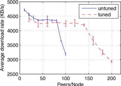
(a) Average download rate

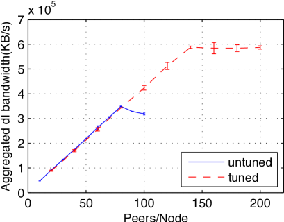
(b) Aggregated download bandwidth

Figure 1: Effects of tuning BitTorrent parameters on average download rate and aggregated bandwidth as a function of peers per node in download-constrained experiments. The bars show 99% confidence intervals.

We can see that the average download rate in the untuned case enters into the stable phase at 40 peers/node (recall that the peer list has 40 peers, as discussed above), and remains stable till it reaches 80 peers/node. After 80 peers/node, the average download rate drops sharply. This change can also be observed clearly on the corresponding aggregated bandwidth in Figure 1(b). Before reaching the system capacity at 80 peers/node, the aggregated bandwidth keeps increasing linearly to 350MB/s. Without tuning the parameters, we can therefore deploy a maximum of 80 peers on a node.

Looking at the curves for the tuned case, we see that the average download rate remains stable until we have 140 peers per node, almost double of that of the untuned case. Likewise, the aggregated bandwidth can reach almost 600 MB/s. In other words, by properly tuning the parameters we can deploy around 140 peers on a node at maximum. The tuned case exhibits similar behavior to the download-constrained case, with a limit of about 140 peers per node.

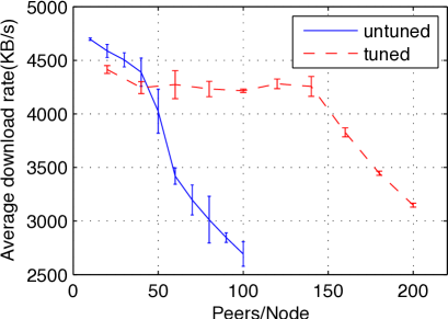
(a) Average download rate

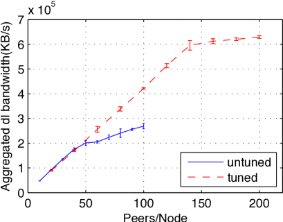
(b) Aggregated download bandwidth

Figure 2: Effects of tuning BitTorrent parameters on average download rate and aggregated bandwidth as a function of peers per node in upload-constrained experiments.

Figure 2 shows the results for upload-constrained experiments, where every leecher had unlimited download rate, but the upload rates were limited to 5 MB/s; seed’s upload was also limited to 5 MB/s as in the previous experiment. The results are similar to the ones from the download-constrained experiment, with the difference that the average download rate for the untuned case never enters a stable phase; instead, after the initial decrease in swarms under 40 peers, it continues to decline, indicating that the system is already overloaded. Interestingly, the aggregated bandwidth still keeps increasing slightly after 40 peers, but as the average download rate indicates, the system is overloaded and the experiment is no longer correct.

Note that the tuned case uses a fixed number of 7 upload slots in both cases. In the upload-constrained case we should actually let BitTorrent decide the number of upload slots according to equation (1). We tried this as well (results shown later in Figures 3(c) and 4) and observed that the behavior is practically identical up to the capacity limit. After the capacity limit has been reached, 7 upload slots means a more stable system performance with a very small variation in average download rate and aggregated bandwidth whereas the real value of 54 slots results in highly variable behavior (Figures 3(c) and 4)

Figures 1(a) and 2(a) show that the average download rate for the tuned case is slightly lower than untuned case when the number of peers is very small. This is because the tuned case uses a larger slice size, hence a piece will be divided into a smaller number of slices. Request pipelining which allows efficient parallel downloads is not as efficient in this case, hence the average download rate suffers slightly, but we have less I/O overhead.

6 Capacity Planning

After determining how the parameters are to be tuned for the best performance, we now turn to the more general issues related to capacity planning. Our goal is to determine general rules of thumb which a system designer can use to evaluate the performance of the system.

First we show that the naive method of only looking at the average download rate is not sufficient, and then we turn to a more elaborate mechanism for estimating the system capacity limit.

6.1 Naive Method For Capacity Planning

In the naive method, we only take average download rate into account. If there is no significant drop in average download rate, then the experiment is considered to be reasonable.

First we experimented with placing all the leechers on a single node. We increased the number of leechers until the average download rate was no longer stable. All leechers were upload-constrained and we used different values for upload bandwidths: 10, 20, 40, and 100 Mbps.

First, we investigated whether we can use the simple formula $y=\frac{a}{x}$ to roughly estimate how many peers we can put on a single node. $y$ is the maximum number of peers we can put on a single node, $x$ is the maximum upload or download rate we set, and $a$ is a constant related to the aggregated bandwidth. If the transmission rate and maximum number of peers on a node exhibit this simple relation, then we need not redo the capacity probing every time we change the experiment settings.

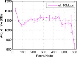
(a) Upload bandwidth 10 Mbps

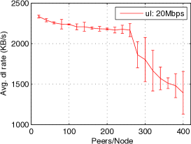
(b) Upload bandwidth 20 Mbps

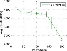
(c) Upload bandwidth 40 Mbps

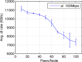
(d) Upload bandwidth 100 Mbps

Figure 3: Average download rate as function of peers per node for different upload bandwidths for case of 1 node being used.

Figure 4: The corresponding aggregated download bandwidth for the cases shown in Figure 3.

Figure 3 plots the average download rate against the number of peers. Even though the maximum upload rates are set to different values, the shapes of the curves are similar. The average download rate decreases slightly until it reaches 40 peers per node, then it enters into a relatively stable stage. After reaching the system capacity, the average download rate drops sharply.

Figure 4 plots the corresponding aggregated download bandwidth based on the same experiment, with the curves from the different cases combined. As the two figures show, the aggregated download bandwidth can increase to 500 MB/s, and the corresponding average download rates remain stable. Thus we can define 500 MB/s of aggregated download bandwidth as the system capacity, and any value below that is considered safe. Since the curves in the safe region are basically straight lines, it is easy to fit a curve and we obtain the result that relation between the number of peers per node, $x$, and maximum upload rate per peer, $y$, is given by

$$y=\frac{560}{x}.$$ (2)

Figure 5 shows this curve and our data points. This curve can be used to set the values for upload bandwidth and number of peers in an experiment when all peers are placed on a single node. In download-constrained experiments, we get similar results as in the upload-constrained experiments.

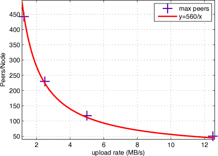
Figure 5: Number of peers/node vs. per-peer upload rate.

6.2 Using More than One Node

We repeated the experiment above by placing the peers on two nodes equally, starting with 20 peers per node and increasing by 20 peers per node until we reached 200 peers per node. Upload rates were constrained to 5 MB/s and download rates were unconstrained. Results for average download rate and aggregated bandwidth are shown in Figure 6 and are at first sight similar to the ones obtained for the single node case (Figure 3(c) and 40 Mbps line in Figure 4).

In a download-constrained experiment, we obtained similar curves (not shown due to space reasons).

Using the naive method, we would be led to conclude that 120 peers per node is still safe, but when we inspected the actual network traffic and connections made by the peers, we noticed that already at 60 peers per node, the network between the nodes had been saturated (see details below). As a result of this saturation, BitTorrent changed its behavior. This is not apparent in Figure 6, hence the naive method is inadequate. Below we provide details about our observations of the changes in behavior and an analytical means for calculating when experiments are still safe.

However, we consider the lack of observed change in the average download rate in changing network conditions as excellent evidence of BitTorrent’s ability to adapt to varying conditions.

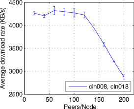
(a) Average download rate

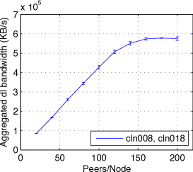
(b) Aggregated download bandwidth

Figure 6: Leechers deployed equally on two nodes; upload-constrained experiment

6.3 Clustering of the Nodes

We will substantiate our above claim that BitTorrent’s behavior has changed and that the average download is not an accurate indicator of a correct experiment in two ways. First, we will experimentally investigate how the connections between the peers are formed in the above experiment. Second, we derive simple analytical expressions for determining the bounds of when an experiment can be considered correct, and demonstrate that the above experiment with two nodes violates these intuitive conditions.

We ran the experiment with two nodes as above, i.e., start with 20 peers per node, increasing it by 20 peers per node until we reach 200 peers per node. Upload rates were constrained to 5 MB/s and download rates were unlimited. In every experiment we kept track of all the connections maintained by all the peers and identified which connections are native (to peers on same node) and which are foreign (to peers on the other node). Every experiment was repeated 3 times and we present the averages and the standard deviations in the figures.

Figure 7 shows the fraction of native buddies in the peer list given by the tracker. As we can see, the value hovers around 50% which is to be expected since the tracker picks the peers for the peer list uniformly at random. Investigating the fraction of native buddies (and consequently foreign buddies) allows us to determine how BitTorrent is choosing where to download from.

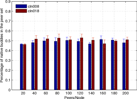
Figure 7: Fraction of native buddies in the peer list

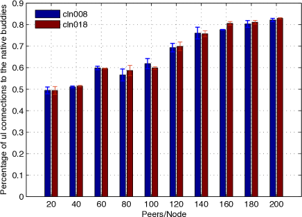
Figure 8: Fraction of upload connections to native buddies in an upload-constrained experiment with 2 nodes

Figure 8 shows the fraction of upload connections to native buddies in an upload-constrained experiment. We used two nodes, cln008 and cln018 and show the values for both of them, as a function of the number of peers per node. As we can see, from 60 peers per node onwards, the peers tend to favor native buddies and the fraction of connections to native buddies keeps on increasing throughout the experiment.

The explanation is quite simple. Because the peers obtained in the peer list are evenly distributed, so are the connections in the smaller tests. Because both the native and foreign peers are able to serve data equally fast, a peer has no reason to prefer one over the other. (Recall that BitTorrent selects the peers to upload to or download from based on the bandwidth it obtains to/from that peer.) At around 60 peers per node, the amount of data going between the nodes is enough to saturate the 1 Gbps network link, whereas the local loopback still has a lot of unused capacity. Hence, what we are seeing in Figure 8 is simply the normal BitTorrent’s peer selection algorithm at work. In other words, the peers have clustered themselves locally but this effect is not visible in the average download rates or aggregate bandwidth shown in Figure 6.

6.4 Clustering with Download Constraints

We repeated the above experiment, but this time constrained the download rate of every leecher to 5 MB/s and left the upload rates unlimited. Seed’s maximum upload rate was 5 MB/s as in the other experiments.

Figure 9 shows the results from this experiment. As with the upload-constrained case, the network is saturated at around 60 peers per node, but the effects are drastically different from the upload-constrained case. The peers start favoring foreign buddies as opposed to native buddies for a longer spell and return to favoring native buddies only in very large experiments.

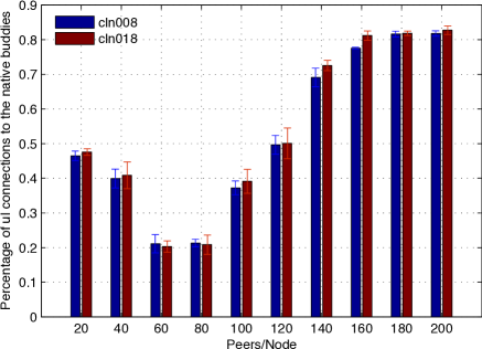
Figure 9: Fraction of upload connections to native buddies in a download-constrained experiment with 2 nodes.

Interestingly, our analysis of the situation showed that although most of the upload connections in the range of 60–80 peers per node were to foreign buddies, the peers received most of the data from native buddies. For example, with 20 peers per node, 54.4% of the traffic came from native buddies, at 60 peers per node this was 60.1% and at 100 peers per node 77.2%. Turns out that this behavior is a result of BitTorrent’s piece selection strategy. Piece selection strategy in BitTorrent is based on a mechanism called rarest-first. The purpose is to make a peer attractive to the others by requesting the rarest pieces first in the swarm, and quickly turn a peer into a productive member of the swarm.

Peers make the decision on which piece they consider to be the rarest based on locally available information from other peers. (This is why in some cases BitTorrent’s piece selection algorithm is called local rarest first.) Peers obtain information about the pieces other peers possess through BitTorrent’s HAVE-control messages. A peer sends a HAVE-message to its buddies when it has completed the download of a piece, in order to let its buddies know that they can download the piece from the peer. Peers keep track of the HAVE-messages and use them to calculate which pieces are the rarest among their buddies.

BitTorrent’s control messages (of which HAVE is one) have to share the network with the actual data transfers. When the network (or loopback device) becomes congested, both the data and control messages are slowed down. At the 60 peers per node point, the network between the nodes starts becoming congested, but the loopback is still far below its capacity. Hence, peers receive a lot of HAVE-messages from the native buddies but the HAVE-messages from foreign buddies slow down. As a result of this, the peer (correctly) considers the pieces from the foreign buddies to be rarer than native pieces (which spread very fast within the node to many peers) and wants to request the rarer pieces from the foreign buddies first. As the network is only approaching the saturation point and is not yet completely congested, the peer is able to provide uploads to foreign buddies so that they are willing to upload pieces to it (recall the use of tit-for-tat).

From the results, we can conclude that BitTorrent’s piece selection algorithm is very sensitive to changes in network conditions in the download-constrained cases. In fact, piece selection strategy overrules peer selection strategy in the early part of the experiment. As the network gets more and more congested, the peers are no longer able to provide good enough upload rates to foreign buddies, so in accordance to the tit-for-tat policy, they are choked. Hence they have to resort to the native buddies for actually getting the data. Since there are no limits on upload rate, the actual injection of new information is limited by the seed’s upload rate (which was limited), but the native buddies are enough to feed new data within the node. Eventually, we see the same kind of clustering between peers on a single node as we saw in the upload-constrained case.

To verify our claim that the behavior above is due to the piece selection algorithm, we repeated the experiment with a random piece selection algorithm. Because peers exhibit no preference for pieces, peer selection algorithm should be the deciding factor. Results are shown in Figure 10. The results are similar to the upload-constrained case in Figure 8 where peer selection is known to be the deciding factor.

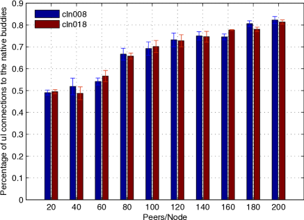
Figure 10: Fraction of upload connections to native buddies in a download-constrained experiment with 2 nodes and random piece selection.

As further evidence, we ran the download-constrained experiment with leechers placed equally on three nodes and the fraction of connections to other nodes is shown in Figure 11. The three parallel bars represent the three nodes. The lowest section of each bar shows native connections and the two upper sections show connections to the two other nodes. We see the same preference for foreign buddies in the beginning, with connections between the other two nodes being rather uniformly split, as is to be expected. After the network gets congested, we see the same kind of clustering as in the case with two nodes.

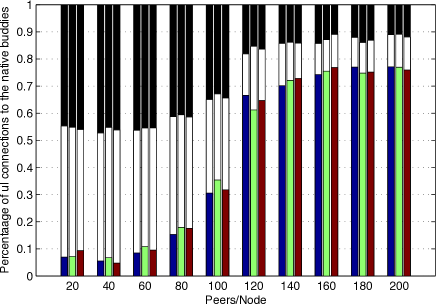
Figure 11: Fraction of upload connections to native buddies (lowest section of bars) and foreign buddies (white and black sections) with 3 nodes in a download-constrained experiment.

6.5 Capacity Planning Formulas

We now present a simple analytical means of determining whether a planned experiment falls within the system capacity limits or not. Table 2 lists the notation used in the following. Let $i,j,k\in\{1,2,3...n\}$. Compared with the traffic among the leechers, the traffic from the seed is negligible and we have excluded it for reasons of simplicity.

$n$	number of nodes in an experiment
$m_{i}$	number of peers on node $i$
$U_{i}$	aggregated upload bandwidth generated by the peers on node $i$
$D_{i}$	aggregated download bandwidth generated by the peers on node $i$
$L_{i}$	physical capacity of loopback device on node $i$
$C^{ul}_{i}$	physical upload capacity of network card on node $i$
$C^{dl}_{i}$	physical download capacity of network card on node $i$
$P_{ij}$	probability that a peer on node $i$ will connect to peers on node $j$

Table 2: variables used in the discussion

When we deploy multiple peers on one node, a peer will not only try to connect and upload to the native peers, but also to the foreign peers. $P_{ij}$ is the probability that a peer on node $i$ will connect to peers on node $j$, and assume all the peers on node $i$ have the same probability. Then we have

$$P_{ij}=\left\{\begin{array}[]{rl}\frac{m_{i}-1}{\sum_{k=1}^{n}m_{k}-1}&\text{if }i=j,\\ \\ \frac{m_{j}}{\sum_{k=1}^{n}m_{k}-1}&\text{if }i\neq j.\end{array}\right.$$ (3)

When $i=j$, $P_{ii}$ actually denotes the probability that a peer will connect to the native peers.

$U_{i}$ and $D_{i}$ denote the aggregated upload and download bandwidth on node $i$ respectively. Obviously, $U_{i}$ equals the sum of all peers’ upload bandwidth on node $i$ and $D_{i}$ equals the sum of all peers’ download bandwidth on node $i$. Then the traffic from node $i$ to node $j$ is

$$T_{ij}=P_{ij}\times min(U_{i},D_{j})$$ (4)

We can construct a matrix to show the traffic flows between the nodes:

$$T=\begin{bmatrix}T_{11}&T_{12}&T_{13}&\ldots&T_{1n}\\ T_{21}&T_{22}&T_{23}&\ldots&T_{2n}\\ \vdots&\vdots&\vdots&\ddots&\vdots\\ T_{n1}&T_{n2}&T_{n3}&\ldots&T_{nn}\\ \end{bmatrix}$$ (5)

In matrix $T$, row $i$ represents the distribution of the traffic flowing out of node $i$, and column $i$ represents the distribution of the traffic flowing into node $i$. The elements on the diagonal represent the traffic going through the loopback interface of a node. This traffic in $T$ must be constrained by the physical capacity of a node. Then for each $i,j$ we have:

$$\sum_{i=1,i\neq j}^{i=n}T_{ij}\leqslant C_{j}^{dl}$$ (6)

$$\sum_{j=1,i\neq j}^{j=n}T_{ij}\leqslant C_{i}^{ul}$$ (7)

$$T_{ii}\leqslant\frac{L_{i}}{2}$$ (8)

Now, consider an extreme situation, when all the traffic goes through loopback interface or the network card, then we have the following constraints:

$$U_{i}\leqslant C_{i}^{ul}$$ (9)

$$D_{i}\leqslant C_{i}^{dl}$$ (10)

$$min(U_{i},D_{i})\leqslant\frac{L_{i}}{2}$$ (11)

To some extent, (6), (7) and (8) define the upper bound of the experiment, while the (9), (10) and (11) define the lower bound. The upper and lower bound will converge at two points. The first is when only one node is used for deploying leechers. Then there is only one element $T_{11}$ in the matrix. The (8) and (11) will be the same, since all the traffic will go through the loopback interface.

The second is when an infinite number of nodes is used. Considering that we can only deploy a limited number of peers on a node, the probability that a peer will connect to native peers decreases to zero. As a result, all the traffic will go through network card. Then (6) and (7) will be the same as (9) and (10). $T_{ii}$ will be zero since no traffic will go through the loopback interface.

6.6 Example: Case of 2 Nodes

We revisit the case of using two nodes in an experiment shown in Figure 6. In the experiment, we obtained an average download rate of 4.25 MB/s and loopback capacity $L_{i}=500$ MB/s. The network between the nodes is a Gigabit Ethernet, so $C_{i}^{ul}=125MB/s$ and $C_{i}^{dl}=125MB/s$. ($i\in\{1,2\}$)

When there are 40 peers on each of the two nodes, we get the traffic distribution matrix $T^{40}$ as below:

$$T^{40}=\begin{bmatrix}T_{11}&T_{12}\\ T_{21}&T_{22}\\ \end{bmatrix}=\begin{bmatrix}83.9&86.1\\ 86.1&83.9\\ \end{bmatrix}$$ (12)

We can see from the equation (12), for node 1, $T_{12}~{}\leqslant~{}C_{1}^{ul}$, $T_{21}~{}\leqslant~{}C_{1}^{dl}$ and $T_{11}~{}\leqslant~{}\frac{L_{1}}{2}$. The same applies to node 2. We can see all the equations hold, the experiments are designed within the system capacity.

When there are 60 peers on each of the two nodes, we obtain the traffic distribution matrix $T^{60}$ as below:

$$T^{60}=\begin{bmatrix}T_{11}&T_{12}\\ T_{21}&T_{22}\\ \end{bmatrix}=\begin{bmatrix}126.4&128.6\\ 128.6&126.4\\ \end{bmatrix}$$ (13)

We can see from the equation (13), for node 1, $T_{12}~{}\textgreater~{}C_{1}^{ul}$ and $T_{21}~{}\textgreater~{}C_{1}^{dl}$. Both equations (6) and (7) are violated. Since equation (11) still holds, then in a upload-constrained experiment, a peer will not treat native buddies and foreign buddies equally. They start showing preference in uploading to native buddies, and the clustering happens. The same analysis can be applied to node 2. This analysis yields the same result as the investigation on the actual behavior of BitTorrent above.

7 Related Work

BitTorrent has been a popular target for research over the past several years, including several papers, e.g., [8, 9, 10, 11, 12] that use a real BitTorrent client in their experiments to validate their models and conclusions. However, less papers have concerned themselves with the accuracy of their experiments and possible bias in their methodologies.

Legout et al. [12, 13] have made a thorough measurement-based research on the two core mechanisms of BitTorrent, piece and peer selection.. However, the influences from these two mechanisms are discussed separately. The authors showed that the rarest first algorithm guarantees a close to ideal entropy, while the choke algorithm guarantees the fairness in the system. None of the results presented in the papers investigate the combined effects of the two mechanisms, which as we have shown, also occurs and can have significant effects on BitTorrent’s behavior.

Antoniu et al. [6] discuss the difficulties in validating large-scale peer-to-peer systems. The authors also proposed a framework for performing large-scale experiments based on grid services. However, how the experiments are affected by the underlying details and the experiment settings are not touched.

However, only a few papers, e.g., [14, 15, 5] concern the accuracy of experiments and the bias of measurements. Work in [15] investigated the sampling bias in BitTorrent experiments. Even though the discussion merely focuses on the approach of using instrumented client to obtain data from real-world swarm, the recommendations proposed in this paper are simple heuristics and guidelines. We have followed their recommendations and have designed our Logger module to follow them. Our Logger module takes a snapshot for the peer every second during its whole life span. This strategy yields very reliable experiment data.

On the other hand, Rasti and Rejaie [14] claim that the data obtained with this approach (injecting an instrumented client into real-world swarm) is not representative and has already been biased in the beginning. The main reason for their claim is that BitTorrent clients tend to cluster with other clients having similar upload bandwidths. This observation is definitely valid for measuring a real-world swarm on the Internet, but as our experiments are performed on a cluster where all peers are instrumented to provide logging information, such a bias does not exist in our experimental setup.

A lot of analytical work has also studied the clustering properties of BitTorrent. Based on the analysis of the choking algorithm, [11] provides empirical evidence of BitTorrent’s clustering and show that peers with similar bandwidths tend to get clustered.

Meulpolder et al. [8] extend an earlier analytical model from [16] and propose a new model for analytical investigation of BitTorrent’s clustering. Their model only takes into account peer selection in BitTorrent and ignores the effects of piece selection. They observe similar clustering behavior as we have observed. However, their model and measurements exhibit a small discrepancy which they conjecture is the result of probabilistic effects from too small experiments. Our results show that clustering in BitTorrent is actually an interplay of both peer and piece selection algorithms, and we believe that their observed discrepancies are a result of their model ignoring piece selection. Although the effects of piece selection on clustering are small and hard to observe, our work, in particular on the download-constrained experiments, has shown that it cannot be ignored. Both [8] and our work find the same effect of upload connections going to foreign peers while the majority of data comes from native peers.

The work by Rao et al. [5] is the closest work to ours. The authors discuss the rationality of performing BitTorrent experiments on a cluster. However, the discussions focus on the marginal influences on the average download rate from various RTT and packet loss rates and conclude that the effects from changing RTTs and packet loss rates are so small that they can be discounted in the evaluation. Our work focuses on how to design an experiment on a cluster properly, i.e., what is the “safe region” for a correct experiment and how BitTorrent behaves when the experiments are performed around the system capacity limit.

The experiment setup in [5] is very similar to the case discussed in our paper. The authors used 3 nodes for deploying leechers (100 leechers on each node) and performed a homogeneous upload-constrained experiment. The maximum upload rate was set to 100 KB/s. They did not consider possible bottlenecks in their experiment setup. Using our capacity planning method from Section 6.5, we can see that their experiments require only on the order of 3 MB/s of bandwidth between nodes and on the loopback. Given that they were using modern computers on the Grid 5000 testbed, they should be well below the system capacity limit. Our work therefore validates their experiment setting as being correct.

8 Conclusion

Experimental evaluation of large scale systems is an important topic in networking research. Currently no ideal environment exists for such evaluations, with simulations, real Internet, and cluster-based testbeds being the commonly used solutions. We believe that cluster-based testbeds offer the best of both worlds, realistic applications with a real (albeit not necessarily realistic) network in between.

In this paper we have shown how to design BitTorrent experiments on a cluster. Our focus has been on identifying how the physical limits of the host machine affect the tests and how many clients can be deployed on a node. We have shown that the number of peers per node depends on many factors, but up to 500 peers per node is realistic for certain values of allocated per-client bandwidth. We have shown that the simple metric of average download rate is not sufficient for determining when an experiment is “safe”, but that a more complex analysis is needed. We provide a simple set of formulas, intended to be used as rules of thumb for determining if an experiment runs into the physical limits of the machine.

Our work has also extended previous work on BitTorrent, by showing that the previously observed clustering behavior is actually a result of both the peer and piece selection algorithms, and not simply the peer selection algorithm as previously believed. Although the effect of the piece selection algorithm is small, it cannot be ignored in all cases.

In our future work, we plan to verify our results using a 10 Gbps network between the nodes. This is likely to change some of the details of our results, since in that case the loopback will saturate before the network; hence the clustering behavior will be different.

References

- [1] L. Peterson, T. Anderson, D. Culler, and T. Roscoe, “A blueprint for introducing disruptive technology into the internet,” SIGCOMM Comput. Commun. Rev., vol. 33, no. 1, pp. 59–64, 2003.
- [2] “PlanetLab Website,” 2010. [Online]. Available: http://www.planet-lab.org/
- [3] “Emulab Website,” 2010. [Online]. Available: http://www.emulab.net/
- [4] “Grid 5000 Website,” 2010. [Online]. Available: http://www.grid5000.fr/
- [5] A. Rao, A. Legout, and W. Dabbous, “Can realistic bittorrent experiments be performed on clusters?” in International Conference on Peer-to-Peer Computing, Aug. 2010.
- [6] G. Antoniu, L. Bougé, M. Jan, and S. Monnet, “Going Large-scale in P2P Experiments Using the JXTA Distributed Framework,” INRIA, Research Report RR-5151, 2004. [Online]. Available: http://hal.inria.fr/inria-00071432/en/
- [7] B. Cohen, “Incentives build robustness in bittorrent,” in Workshop on Economics of Peer-to-Peer systems, 2003.
- [8] M. Meulpolder, J. Pouwelse, D. Epema, and H. Sips, “Modeling and analysis of bandwidth-inhomogeneous swarms in bittorrent,” in International Conference on Peer-to-Peer Computing, sep. 2009, pp. 232 –241.
- [9] R. Kumar and K. Ross, “Peer-assisted file distribution: The minimum distribution time,” in Hot Topics in Web Systems and Technologies, nov. 2006, pp. 1 –11.
- [10] M. Sirivianos, J. Han, P. Rex, and C. X. Yang, “Free-riding in bittorrent networks with the large view exploit,” in Intenational Workshop on Peer-to-Peer Systems, 2007.
- [11] A. Legout, N. Liogkas, E. Kohler, and L. Zhang, “Clustering and sharing incentives in bittorrent systems,” in ACM SIGMETRICS. New York, NY, USA: ACM, 2007, pp. 301–312.
- [12] A. Legout, G. Urvoy Keller, and P. Michiardi, “Understanding BitTorrent: An Experimental Perspective,” INRIA Sophia Antipolis, Technical Report, 2005. [Online]. Available: http://hal.inria.fr/inria-00000156/en/
- [13] A. Legout, G. Urvoy-Keller, and P. Michiardi, “Rarest first and choke algorithms are enough,” in Internet Measurement Conferences. New York, NY, USA: ACM, 2006, pp. 203–216.
- [14] A. Rasti and R. Rejaie, “Understanding peer-level performance in bittorrent: A measurement study,” in International Conference on Computer Communications and Networks, aug. 2007, pp. 109 –114.
- [15] B. Zhang, A. Iosup, and et al, “Sampling bias in bittorrent measurements,” in Euro-Par, 2010.
- [16] D. Qiu and R. Srikant, “Modeling and performance analysis of bittorrent-like peer-to-peer networks,” in ACM SIGCOMM. New York, NY, USA: ACM, 2004, pp. 367–378.