Uncertainties in grid-based estimates of stellar mass and radius

Abstract

Context. The availability of high-quality astero-seismological data provided by satellite missions stimulated the development of several grid-based estimation techniques to determine the stellar masses and radii. Some aspects of the systematic and statistical errors affecting these techniques have still not been investigated well.

Aims. We study the impact on mass and radius determination of the uncertainty in the input physics, in the mixing-length value, in the initial helium abundance, and in the microscopic diffusion efficiency adopted in stellar model computations.

Methods. We consider stars with mass in the range [0.8 - 1.1] $M_{\sun}$ and evolutionary stages from the zero-age main sequence to the central hydrogen exhaustion. To recover the stellar parameters, a maximum-likelihood technique was employed by comparing the observations constraints to a precomputed grid of stellar models. Synthetic grids with perturbed input were adopted to estimate the systematic errors arising from the current uncertainty in model computations.

Results. We found that the statistical error components, owing to the current typical uncertainty in the observations, are nearly constant in all cases at about 4.5% and 2.2% on mass and radius determination, respectively. The systematic bias on mass and radius determination due to a variation of $\pm 1$ in $\Delta Y/\Delta Z$ is $\pm 2.3\%$ and $\pm 1.1\%$; the one due to a change of $\pm 0.24$ in the value of the mixing-length $\alpha_{\rm ml}$ is $\pm 2.1\%$ and $\pm 1.0\%$; the one due to a variation of $\pm 5\%$ in the radiative opacity is $\mp 1.0\%$ and $\mp 0.45\%$. An important bias source is to neglect microscopic diffusion, which accounts for errors of about 3.7% and 1.5% on mass and radius. The cumulative effects of the considered uncertainty sources can produce biased estimates of stellar characteristics. Comparison of the results of our technique with other grid techniques shows that the systematic biases induced by the differences in the estimation grids are generally greater than the statistical errors involved.

1 Introduction

Accurate and precise determination of the main stellar parameters is fundamental in many astrophysical areas. The continuously growing number of detected extrasolar planets over the past decade has strengthened this statement even more, since the inferred properties of a planet depend on the mass and radius estimates of the host star.

The growth of observational asteroseismology through satellite missions, such as CoRoT (see e.g. Appourchaux et al. 2008; Michel et al. 2008; Baglin et al. 2009) and Kepler (see e.g. Borucki et al. 2010; Gilliland et al. 2010), has opened a new way to estimate stellar properties of solar-type stars, such as mass, radius, and age. Moreover, these properties can be determined more precisely by combining these data with traditional non-seismic observables, such as effective temperature $T_{\rm eff}$, metallicity [Fe/H], and luminosity $L$.

Different techniques of analysis have been developed to exploit the growing availability of data. Some of them attempt a direct fit to the individual oscillation frequencies (Metcalfe et al. 2009), while others determine the stellar parameters by fitting the data to precomputed grid of stellar models (see e.g. Stello et al. 2009; Basu et al. 2010; Quirion et al. 2010; Gai et al. 2011; Huber et al. 2013). These methods have been recently adopted in stellar population studies (see e.g. Chaplin et al. 2011; Verner et al. 2011; Mathur et al. 2012; Miglio et al. 2012) because they allow a fast and automated way to obtain the stellar characteristics from data.

Although a large amount of work has been done to determine the systematic and statistical errors inherent in grid-based estimates (see e.g. Gai et al. 2011; Basu et al. 2012), some aspects have still not been investigated thoroughly. In particular, the impact of the current uncertainty in the main input physics required to compute the stellar models at the base of any grid technique has not yet been quantified fully. In Valle et al. (2013a, b) we showed that the effect on stellar evolutionary tracks and isochrones of the uncertainties in the microphysics input (i.e. radiative opacity, nuclear reaction cross sections, etc.) adopted in stellar codes is not negligible. Thus, to evaluate the reliability of the values obtained using any grid technique, it is necessary to understand how the uncertainties in microphysics propagate into the final results. Besides the input physics, the stellar models depend on the values of some still uncertain parameters, such as the initial chemical abundances (i.e. the initial helium abundance at a given metallicity) and the efficiency of the convective transport, i.e. the mixing-length parameter and the core overshooting (Chaboyer et al. 1995; Barmina et al. 2002; Claret 2007).

In this paper we address the problem of quantifying the effects of those uncertainties affecting stellar models on the star properties derived from a grid technique. We restrict our analysis to central hydrogen-burning stars with mass in the range [0.8 - 1.1] $M_{\sun}$. We focus on the following uncertainty sources: the radiative opacity, the microscopic diffusion velocities, the ¹⁴N$(p,\gamma)^{15}$O reaction rate, the mixing-length parameter value, and the initial helium abundance-metallicity relationship. The uncertainty in the convective core overshooting extension is neglected, since the stars in the chosen mass range burn hydrogen in a radiative core.

The structure of the paper is the following. In Sect. 2, 3 we discuss the method and the grids used in the estimate process; in Sect. 4 we discuss the effects on the estimates of the grid morphology; the main results are presented in Sects. 5 - 7; in Sects. 8 and 9 we present a comparison of the estimates obtained with our grids with some observations and with those obtained by other techniques. Some concluding remarks can be found in Sect. 10.

2 Grid-based recovery technique

We developed a code – SCEPtER (Stellar CharactEristics Pisa Estimation gRid) – that allows, through a maximum likelihood technique, to estimate the stellar mass and radius given a set of observable quantities relying on a grid of precomputed stellar models. The code is quite flexible since different observables can be used, depending on their availability, as well as different grids of models. The code and the grids developed for this work are available in the R packages SCEPtER and SCEPtERextras on CRAN.

In the current paper we focus on the case where four quantities are available: the stellar effective temperature $T_{\rm eff}$, the metallicity [Fe/H], the large frequency spacing $\Delta\nu$, and the frequency of maximum oscillation power $\nu_{\rm max}$. The large frequency spacing $\Delta\nu$ is the spacings between consecutive overtones having the same spherical angular harmonic, and they are related to the acoustic radii of the stars (see e.g. Christensen-Dalsgaard 2012, and references therein). The frequency of maximum oscillation power $\nu_{\rm max}$ is related to the acoustic cut-off frequency of a star (see e.g. Chaplin et al. 2008). The selection of these seismic parameters is motivated by their being recovered from most of target stars.

More in detail, we adopted the same scheme described in Basu et al. (2012). We let $\cal S$ be a star for which the following vector of observed quantities is available: $q^{\cal S}\equiv\{T_{\rm eff,\cal S},{\rm[Fe/H]}_{\cal S},\Delta\nu_{\cal S},\nu_{\rm max,\cal S}\}$. Then we let $\sigma=\{\sigma(T_{\rm eff,\cal S}),\sigma({\rm[Fe/H]}_{\cal S}),\sigma(\Delta\nu_{\cal S}),\sigma(\nu_{\rm max,\cal S})\}$ be the nominal uncertainty in the observed quantities. For each point $j$ on the estimation grid of stellar models, we define $q^{j}\equiv\{T_{{\rm eff},j},{\rm[Fe/H]}_{j},\Delta\nu_{j},\nu_{{\rm max},j}\}$. Let ${\cal L}_{j}$ be the likelihood function defined as

$${\cal L}_{j}=\left(\prod_{i=1}^{4}\frac{1}{\sqrt{2\pi}\sigma_{i}}\right)\times\exp\left(-\frac{\chi^{2}}{2}\right)$$ (1)

where

$$\chi^{2}=\sum_{i=1}^{4}\left(\frac{q_{i}^{\cal S}-q_{i}^{j}}{\sigma_{i}}\right)^{2}.$$ (2)

The technique allows an easy expansion whenever other observational constraints are available, since they can be inserted into the same scheme.

The likelihood function is evaluated for each grid point within $3\sigma$ of all the variables from $\cal S$, allowing for a faster computation without introducing any perturbation on the estimated quantities. We then let

$${\cal L}_{\rm max}=\max_{j}{\cal L}_{j}$$ (3)

be the maximum value of the likelihood function over the estimation grid of stellar models. The estimated values of radius and mass are obtained by averaging the radius and the mass of all the models with likelihood greater than $0.95\times{\cal L}_{\rm max}$.

Whenever an informative prior on the stellar characteristics to be estimated is available, the technique can take the information into account in the likelihood computation. The prior can be inserted as a multiplicative factor in Eq. (1), and it can be considered as a weight attached to the grid points.

The technique can also be employed to construct a confidence interval for mass and radius estimations. To this purpose a synthetic sample of $n$ stars is generated, following a multivariate normal distribution with vector of mean $q^{\cal S}$ and covariance matrix $\Sigma={\rm diag}(\sigma)$. A value of $n=10000$ is usually adopted since it provides a fair balance between computation time and the accuracy of the results. The median of the radius and mass of the $n$ objects is taken as the best estimate of the true values; the 16th and 84th quantiles of the $n$ values are adopted as a $1\sigma$ confidence interval.

2.1 Standard estimation grid

The standard estimation grid of stellar models is obtained using our well tested evolutionary code – FRANEC (Degl’Innocenti et al. 2008) – in the same configuration as was adopted to compute the Pisa Stellar Evolution Data Base for low-mass stars (Dell’Omodarme et al. 2012; Dell’Omodarme & Valle 2013).

The grid consists of 78320 points (110 points for 712 evolutionary tracks), corresponding to evolutionary stages from the ZAMS to central hydrogen exhaustion. Models are computed for masses in the range [0.80 - 1.10] $M_{\sun}$ with a step of 0.01 $M_{\sun}$ and [Fe/H] in the range [$-0.55$ - 0.55] with a step of 0.05 dex. The solar scaled heavy-element mixture by Asplund et al. (2009) is adopted. The initial helium abundance is obtained using the linear relation:

$$Y=Y_{p}+\frac{\Delta Y}{\Delta Z}Z$$ (4)

with cosmological ⁴He abundance value $Y_{p}=0.2485$ from WMAP (Cyburt et al. 2004; Steigman 2006; Peimbert et al. 2007a, b), and assuming $\Delta Y/\Delta Z=2$ (Pagel & Portinari 1998; Jimenez et al. 2003; Gennaro et al. 2010). The models are computed assuming the solar-scaled mixing-length parameter $\alpha_{\rm ml}=1.74$. Present calculations use the most recent version of the OPAL equation of state, EOS 2006 (Rogers et al. 1996; Rogers & Nayfonov 2002). Radiative opacity coefficients are taken from the OPAL group (Iglesias & Rogers 1996) in the version released in 2006 for temperatures higher than $10^{4.5}$ K, and from Ferguson et al. (2005) for lower temperatures. Nuclear reaction rates are taken from the NACRE compilation (Angulo et al. 1999) except for ¹⁴N$(p,\gamma)^{15}$O, for which we adopt a more recent estimate by Imbriani et al. (2005). Present models include atmospheric models by Brott & Hauschildt (2005) as outer boundary conditions. Atomic diffusion is included, taking the effects of gravitational settling and thermal diffusion into account with coefficients given by Thoul et al. (1994). Further details on the input adopted in the computations are available in Valle et al. (2009).

The average large frequency spacing $\Delta\nu$ and the frequency of maximum oscillation power $\nu_{\rm max}$ are obtained using a simple scaling from the solar values:

$$\frac{\Delta\nu}{\Delta\nu_{\sun}} = \sqrt{\frac{M/M_{\sun}}{(R/R_{\sun})^{3}}}\quad,$$ (5)

$$\frac{\nu_{\rm max}}{\nu_{\rm max,\sun}} = \frac{{M/M_{\sun}}}{(R/R_{\sun})^{2}\sqrt{T_{\rm eff}/T_{\rm eff,\sun}}}.$$ (6)

In the case of $\Delta\nu$, a more accurate approach would require the fit of the pulsational frequencies of each model, but the extraction of frequencies is generally only possible for high signal-to-noise detections. Moreover, it has been shown (Stello et al. 2009; Basu et al. 2010) that the simple scaled values are adequate for the grid-estimation process. For a review of both theoretical and empirical tests of Eqs. 5 and 6 we refer to Belkacem (2012); Miglio et al. (2013), and to Sect. 2.1 of Huber et al. (2013).

3 Grid technique internal accuracy

To test the consistency of the recovery procedure, we built a synthetic dataset by sampling $N=10000$ artificial stars from the same standard estimation grid of stellar models used in the recovery procedure, adding to each of them a Gaussian noise in all the observed quantities. We assumed the same standard deviations as used by Gai et al. (2011): i.e. 2.5% in $\Delta\nu$, 5% in $\nu_{\rm max}$, 100 K in $T_{\rm eff}$, and 0.1 dex in [Fe/H].

The recovery of mass and radius for these artificial stars by adopting the same standard grid as was used to generate them will reveal possible distortions introduced by the technique itself and will serve as reference for all the other results. This numerical experiment will prove the performances of our grid technique in the ideal case where the adopted stellar models are in perfect agreement with real stars.

Figure 1: (Top) Kernel density estimate of the relative error for mass reconstruction (bandwidth 0.0060). (Bottom) As the upper panel but for the radius (bandwidth 0.0031). Stars are sampled and reconstructed on the standard grid. A positive value of the relative error indicates an estimated value greater than the true value.

In Fig. 1 we present the kernel density estimates of the relative error for the mass and radius reconstruction (Scott 1992; Venables & Ripley 2002). Some details on the adopted technique are given in Appendix A. In all the cases a positive value of mass (radius) relative error indicates an estimated value greater than the true value. The relevant quantities of the distributions are summarized in rows 1 (labelled “standard”) of Table 1. In the table we report, for mass and radius relative errors, the median of the distribution; the width of its 95% confidence interval; the standard deviation of the data; the width of its 95% confidence interval; the 16th and 84th quantiles of the data. For ease of identification, each case is identified by a number and a label, which are identical for mass and radius.

Since the median of the relative error of mass and radius estimates are consistent with zero, the technique is unbiased for the standard case (i.e. the technique is accurate). The standard deviation values for the mass and radius estimates are of the order of, respectively, 4.5% and 2.2%, so the method provides good recovery precision; however, the error on the single estimate can be as much as 20% and 10% for mass and radius, respectively.

Table 2 gives the standard deviation of the relative errors in the mass and radius estimates for different assumptions on the adopted errors in the observed quantities. This allow to explore the sensitivity of the reconstruction procedure to the precision degree of the observational data. As a first test, lines 1 in Table 2 show the effect of doubling the precision of effective temperature measurements (i.e. 50 K as $T_{\rm eff}$ error) and keeping the uncertainties in the other quantities fixed to the standard value. As a second test, lines 2 in Table 2 show the impact of halving the error in metallicity measurements (i.e. 0.05 dex as [Fe/H] error), again adopting the standard value for the uncertainty in the other quantities. The third test assumes 1% in $\Delta\nu$ and 2.5% in $\nu_{\rm max}$ (lines 3 in Table 2). The last test (lines 4 in Table 2) assumes the set of all reduced errors quoted above.

Concerning mass reconstruction, increasing the $T_{\rm eff}$ precision of a factor of two has a major effect on the reconstructed mass, as it leads to a reduction of the standard deviation on relative errors from 4.5% to 3.5%. The second most important effect is due to improving the metallicity measurements, whereas having more precise $\Delta\nu$ and $\nu_{\rm max}$ only leads to a minor improvement. This behaviour can be understood by considering the mass gradient with respect to $T_{\rm eff}$ and seismic parameters in the neighbourhood of a reference point. It turns out that the dependence of mass on $T_{\rm eff}$ is much steeper than the one on seismic parameters. The stellar tracks for the evolutionary stages considered in this paper evolve at slightly changing $T_{\rm eff}$, but rapidly decreasing seismic parameters (see e.g. the right panel in Fig. 3).

Regarding radius determination, increasing the precision in the two asteroseismic observables has the strongest impact, reducing the standard deviation on relative errors from 2.2% to 1.6%. More precise effective temperature and metallicity measurements only lead to a small improvement in radius precision. All these results agree with those of Basu et al. (2012). The set of all reduced errors roughly halves the standard deviation of the mass and radius estimates.

Figure 2: (Upper row) Dependence of mass estimate relative errors on the true mass of the star, on the metallicity value, [Fe/H], and on the relative age of the star (see text). The [Fe/H] is the surface value currently present for the star, not the original one. (Lower row) The same as upper row but for radius reconstruction. Data are sampled and reconstructed on the standard grid of stellar models. The black lines represent a LOWESS smoother of the data. A positive value for the relative error indicates an estimated value greater than the true value.

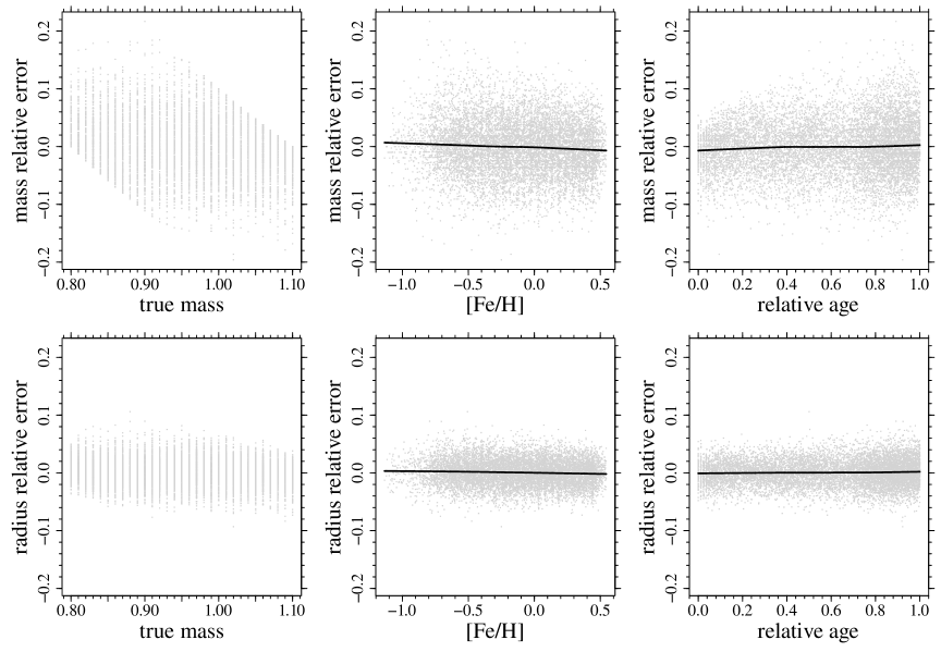
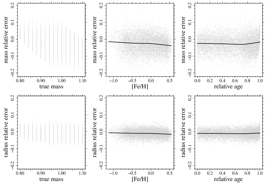
Figure 2 shows the dependence of relative errors on the recovered mass and radius on the true stellar mass, [Fe/H] value, and relative age, defined as the ratio between the age of the star and the age of the same star at central hydrogen exhaustion. (The age is conventionally set to 0 at the ZAMS position.) The ratio [Fe/H] is the current surface value for the star, which can be significantly different from the initial one owing to the microscopic diffusion processes. The figure shows a LOWESS (LOcally Weighted Scatterplot Smoothing) smoother of the data (Cleveland 1981). More details on the technique are given in Appendix A.

The most evident feature is the ”edge effect” that characterizes the trend of the mass relative errors versus the true mass of the stars. The trend is a distinctive feature of a maximum likelihood grid technique, although its relevance is not always recognized. This is because the mass can never be estimated at values outside the grid, so that the estimate of the mass of a star with true mass of 0.80 $M_{\sun}$, the lowest value available in the grid, can never result in values below 0.80 $M_{\sun}$. The opposite occurs for a star of true mass 1.10 $M_{\sun}$, our highest value; i.e. the estimated mass can never result in a value greater than 1.10 $M_{\sun}$. As a consequence the apparent precision of mass estimate on the grid is higher toward its edges, but these estimates are systematically biased. Very similar behaviour is reported, for instance, in Gai et al. (2011) (their Fig. 9) although its causes are not discussed.

As shown in the left-hand panel of the bottom row in Fig. 2, the same effect, although less evident, is present in the decreasing trend of the radius relative errors versus the true mass of the stars. In this case the trend is induced by the fact that the radius of a star increases with the star mass, so that for the lowest mass (0.80 $M_{\sun}$) the probability of having an estimate of radius below the edge of the grid is null, while it is possible to have radius estimate above the grid values spanned by 0.80 $M_{\sun}$ models, because of the increasing trend mentioned above. The reverse behaviour occurs for 1.10 $M_{\sun}$ models. A more detailed discussion of the edge effects can be found in the next section.

Interestingly, no clear trend is shown for different values of [Fe/H]. The region at [Fe/H] ¡ $-0.8$ dex is poorly populated since the microscopic diffusion can reduce the surface [Fe/H] at these values only for a few tracks that start at low metallicity. For the dependence on relative age, a mild increase in the standard deviation is found for the mass estimate: from a value of 0.037 for relative ages in the range [0.00 - 0.25] to a value of 0.049 in the range [0.75 - 1.00]. This is another example of the edge effect, a pervasive presence in several aspects of the grid-based estimation. More details on this topic are given in Sect. 4.

As a last comment, as reported in the literature (see e.g. Jørgensen & Lindegren 2005), neglecting the evolutionary time step in grid-based calculations can lead to significant biases in the estimated stellar parameters. However, the mass range adopted in our computations – which stops at 1.10 $M_{\sun}$ – including metallicity and seismic constraints and excluding the PMS and post central hydrogen exhaustion phases, reduce the occurrence of intersecting tracks. To quantify the bias, we performed a weighted grid estimate of mass, using the evolutionary age as weight. Only a small median bias of -0.003 $M_{\sun}$, which is constant for all ages, is found. No relevant differences appear for the relative error in mass estimates.

4 Trends induced by the grid morphology

In Sect. 3 a mild trend in the standard deviation of the relative errors on mass estimates with the relative age of the star is reported . Although the effect is very small for most practical purposes, it deserves analysis since it is typical of grid-based estimation techniques. Such an effect is related to the morphology of the projection of the grid in the ($T_{\rm eff}$, $\Delta\nu$) and in the ($T_{\rm eff}$, $\nu_{\rm max}$) planes. To keep the discussion simple and to increase the relevance of the effect under investigation, we focus on the case where only $T_{\rm eff}$ and $\Delta\nu$ (or equivalently $\nu_{\rm max}$) are available.

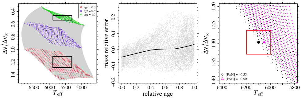
In the left-hand panel of Fig. 3, we plot the projection of the estimation grid in the ($T_{\rm eff}$, $\Delta\nu$) plane. The evolutionary path of a star starts at the bottom edge of the grid and develops towards lower values of $\Delta\nu$. In the figure we display the position of the ZAMS points, of the points that mark the 80% of the evolution, and of the final points corresponding to the central hydrogen depletion.

The figure shows that during the evolution of a MS star, a slight variation in$T_{\rm eff}$ corresponds to a large decrease in $\Delta\nu$. It also appears that the points corresponding to the models with relative ages 0.0 and 0.8 are more scattered in $\Delta\nu$ than those with relative age 1.0. Moreover, the separation in $\Delta\nu$ of regions at given relative ages increases as a star evolves from the ZAMS towards the central-hydrogen exhaustion. In fact, as shown in the left-hand panel of Fig. 3, the $\Delta\nu$ decrease from the ZAMS to the models with relative age 0.8 is nearly the same of the decrease from the model with relative age 0.8 to the one corresponding to central-hydrogen exhaustion. Furthermore, the dimension of the $3\sigma$ boxes around a point shrinks in $\Delta\nu$ at later ages, since the error on seismic quantities is assumed to be a fixed percent of the seismic values. This effect is shown in the figure.

In the middle panel of Fig. 3 we display the relative error on mass estimates versus the relative age of the stars. The increase in the variance with relative age is much more evident than in the case discussed in Sect. 3, where the availability of the metallicity on the estimation procedure mitigates the effect. The trend is due to the different probability of selecting an object of mass higher or lower than the one of the sampled object in the maximum likelihood analysis. This is shown in the right-hand panel of Fig. 3. It is clear that most of the models encompassed by the $1\sigma$ box correspond to mass lower (at lower $T_{\rm eff}$) than the reference case one. Moreover, tracks corresponding to lower masses enter in the box at later stages of evolution than tracks corresponding to higher masses. The conclusion holds even if tracks at different metallicity are included. As a result the mass is generally underestimated for low values of relative age. To help estimate the effects, we note that the relative age of 0.20 is reached at around the 18th point of the track.

Figure 3: (Left): region of the ($T_{\rm eff}$, $\Delta\nu$) plane spanned by the reconstruction grid; the points mark the position of ZAMS (red), of the relative evolutionary age 0.8 (blue), and of the central hydrogen depletion (green). The black boxes show the typical extent of the $3\sigma$ regions in the initial and final stages of the stellar evolution. (Middle): relative error on mass estimates with respect to the relative age of the stars. Only $T_{\rm eff}$ and $\Delta\nu$ are employed for the estimate. (Right): detail of the region around the $M$ = 0.90 $M_{\sun}$ (black dot) for initial [Fe/H] = $-0.55$. The red box shows the extent of $1\sigma$ region around the aforementioned model. The magenta diamond corresponds to the same model for initial [Fe/H] = $-0.50$. The dashed line marks the evolutionary path of the model.

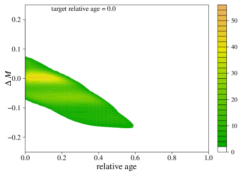
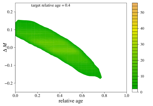
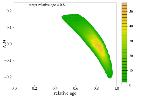
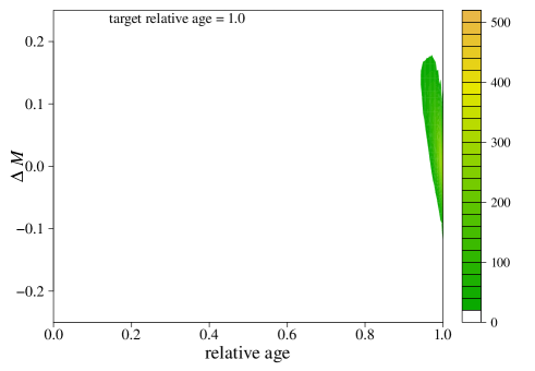
As we move to higher relative ages, the mass underestimation disappears, and the standard deviation of the mass relative error estimates increases. To understand this increase we refer to the case treated in Sect. 3 and assume that the metallicity of the star is available, along with $T_{\rm eff}$ and seismic parameters. We selected the reference points corresponding to target relative ages 0.0, 0.4, 0.8, and 1.0 in the grid. We then considered all the models in the $3\sigma$ boxes of the reference points and computed, for the four reference ages separately, the quantity $\Delta M$ defined as the difference between the mass of the reference point and the mass of the models in the box.

In Fig. 4 we plot the joint density of $\Delta M$ and relative age of all the models at the four selected target relative ages. The density of the extreme cases (target relative age 0.0 and 1.0) are strongly peaked in mass, in particular for the case at late age. It is also apparent the effect induced by the edge of the grid, mainly at target relative age 0.0, where the distribution toward higher masses is truncated at the grid edge. In the middle and third quarters of the evolution (i.e. relative ages 0.4 and 0.8, respectively), the mass densities are flatter, so the variances are higher than in the previous two cases. In other words, at intermediate relative ages, the grid is populated by models covering a mass range that is wider than in the other two cases.

The trend and the asymmetries of Fig. 4 are the consequences of stellar evolution. The changes are smooth in the first part of the evolution; the seismic quantities evolve faster in the later stages, after about relative age 0.8. In fact, as discussed above, in the first three quarters of the evolution, the reference points in each reference level span a wide hyper-range, and the levels are close one another (see left panel, Fig. 3). At late evolutionary stages, they pack more closely in each levels and separate strongly from one another. As a consequence, at late relative ages, a $3\sigma$ box around the reference point contains more homogeneous grid models, i.e. models with more similar masses and relative ages than in the early evolution.

Figure 4: Joint density of $\Delta M$ and relative ages selected in the $3\sigma$ boxes around the references point for target relative ages 0.0, 0.4, 0.8, and 1.0. A positive value of $\Delta M$ implies that the selected mass is greater than the reference one. The color legend of the lower right panel is different from the others because the distribution is much more peaked.

5 Stellar-model uncertainty propagation

The accuracy and precision of the parameters of real stars inferred by means of any grid-based technique depend on the reliability degree of the adopted stellar models. The evolutionary tracks, hence the grid-based results, are susceptible to variations arising from the adopted input physics (radiative opacity, nuclear reaction cross-sections, etc.), efficiency of macroscopic processes (e.g. convection), and initial chemical composition.

For the first issue, we have recently shown that the cumulative uncertainty affecting the current generation of stellar models from the combined effect of the main input physics is still not negligible (see e.g. Valle et al. 2013a, b, for a detailed discussion). Regarding the second point, it is well known that the rough treatment of super-adiabatic convective transport is one of the major weakness in stellar computations. This means that the predicted effective temperature of stars with a convective envelope strongly depends on the adopted value of the mixing-length parameter. Finally, stellar tracks and isochrones clearly depend on the initial chemical composition adopted in the computations.

The variations of the stellar tracks due to all the uncertainty sources mentioned above will affect the estimates obtained from grid techniques in a non-trivial way, owing to the concurrent effects arising from a single ingredient variation. Direct estimates obtained from perturbed stellar models are the only way to tackle the problem.

To this purpose we computed several sampling grids of non-standard stellar tracks, with mass steps of 0.02 $M_{\sun}$, adopting perturbed input physics, different values of the helium abundance at a given metallicity, and various mixing-length parameters $\alpha_{\rm ml}$. From these non-standard grids we sampled the corresponding synthetic datasets of $N=10000$ artificial stars. We applied to these datasets our recovery procedure based on the standard grid of stellar models in order to estimate mass and radius of the artificial objects as in the case of real data. Comparing these reconstructed values with the known true ones allows the effect of the various uncertainty sources discussed in detail to be quantified in the following sections.

5.1 Initial helium abundance

The observable quantities of a star of given age and mass depend on its chemical composition. While the surface metallicity can be measured, the helium abundance cannot be determined for the vast majority of stars, since helium lines are not observable in stars colder than about 20000 K. From the theoretical point of view, this means that one has to assume an initial value $Y$ for the helium abundance to adopt in stellar evolution computations. The common procedure consists in assuming the linear relationship between the original helium $Y$ and metallicity $Z$ shown in Eq. (4). However, the value of the helium-to-metal enrichment ratio $\Delta Y/\Delta Z$ is still quite uncertain (Pagel & Portinari 1998; Jimenez et al. 2003; Gennaro et al. 2010), since its determination relies only on indirect methods. Such an uncertainty directly translates into an uncertainty in the initial helium abundance adopted in stellar computations for a given initial metallicity and, in turn, into an uncertainty in the predicted observable quantities of a star.

Figure 5: Median of mass and radius relative errors; the error bars correspond to their 95% confidence interval. The synthetic data are sampled from grids of stellar models with $\Delta Y/\Delta Z$ = 1, 2, 3 and reconstructed on the standard grid with $\Delta Y/\Delta Z$ = 2.

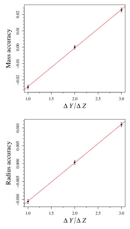
To quantify the impact of a change in the star’s initial helium content on the estimate of its mass and radius, we computed two additional grids of stellar models with the same values of the metallicities $Z$ as in the standard grid but by changing the helium-to-metal enrichment ratio in Eq. (4) within the current uncertainty, namely $\Delta Y/\Delta Z$ = 1 and 3. Then, we built a synthetic dataset of $N=10000$ artificial stars by sampling the objects from the non-standard grid with $\Delta Y/\Delta Z=1$ and another from the non-standard grid with $\Delta Y/\Delta Z=3$. The mass and radius of the objects are then estimated using the recovery procedure based on the standard grid. The results of these tests are presented in rows 2-3 of Table 1 and in Fig. 5. The figure shows the values of the median of the relative error in mass and radius estimates, where the error bars show their 95% confidence interval. The lines represent the weighted least squares fit to the values.

It appears that the effect of changing the initial helium abundance is highly symmetric around the standard value, which corresponds to the case discussed in Sect. 3. The bias induced by the considered uncertainty in initial helium abundance is of the order of $\pm$2.3% on mass estimates and $\pm$1.1% on the radius. As expected, an increase (decrease) in the initial helium content of the stars shifts the mass estimate to higher (lower) values. In fact, with respect to the standard grid models, the helium-rich ones have higher effective temperature and radius, and consequently lower seismic parameters. Recalling that as the mass increases, $T_{\rm eff}$ increases, whereas seismic parameters decrease, it follows that the mass of the sampled object will generally be overestimated. In this case the grid technique shows a bias, although the statistical errors, represented by the standard deviation, are still dominant on average (but see e.g. discussion below on metal-rich stars).

Figure 6: As in Fig. 2, but for data sampled from a grid with $\Delta Y/\Delta Z=1$, and recovered with the standard grid adopting $\Delta Y/\Delta Z=2$.

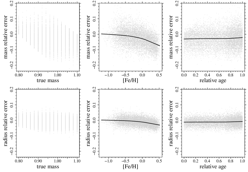
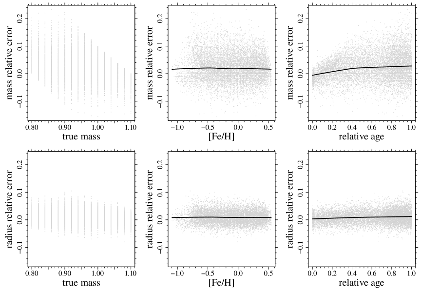
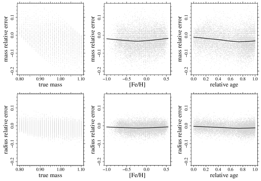
Figure 6 shows the same quantities as Fig. 2 but for the case of synthetic data sampled from stellar models adopting $\Delta Y/\Delta Z=1$. Apart from the trend with mass discussed above, there is a signature of an edge effect in the trends on relative age, similar to the one discussed in Sect. 4. The most interesting feature is, however, a clear metallicity effect. This is because $Y$ and $Z$ are linked by the relation in Eq. (4) so that at low $Z$ values the change in $Y$ driven by a change in $\Delta Y/\Delta Z$ is less than the same change at high metallicity.

As a result, the uncertainty in helium content mainly affects stars at high values of [Fe/H]: the median of the distribution of mass relative errors is $-0.005$ for [Fe/H] $\leq$ $-0.5$, $-0.016$ in the range of [Fe/H] = [$-0.5$, 0.0], and it grows to a value of $-0.048$ for [Fe/H] $\geq$ 0.0. The last error is comparable to the standard deviation of mass relative-error distribution.

The effect of helium uncertainty should then be carefully taken into account if the technique is applied to metal-rich objects, since it can result in biased estimates of mass and radius. The trend discussed above is reversed whenever the initial helium content is increased with respect to the standard grid (plots with $\Delta Y/\Delta Z=3$ not shown).

5.2 Mixing-length value

The lack of a solid and fully consistent treatment of the convective transport in superadiabatic regimes prevents modern stellar evolution codes to firmly predict the effective temperature and radius of stars with an outer convective envelope, such as those studied in this paper. The common approach consists in adopting a simplified treatment as the mixing-length theory, where the efficiency of the convective transport depends on a free parameter $\alpha_{\rm ml}$ to be calibrated with observations. Usually, stellar models adopt the solar calibration that in our standard case provides $\alpha_{\rm ml}=1.74$. Nevertheless, there is no stringent a priori reason that guarantees that the solar calibrated $\alpha_{\rm ml}$ value is also suitable for stars of different masses and/or in different evolutionary stages.

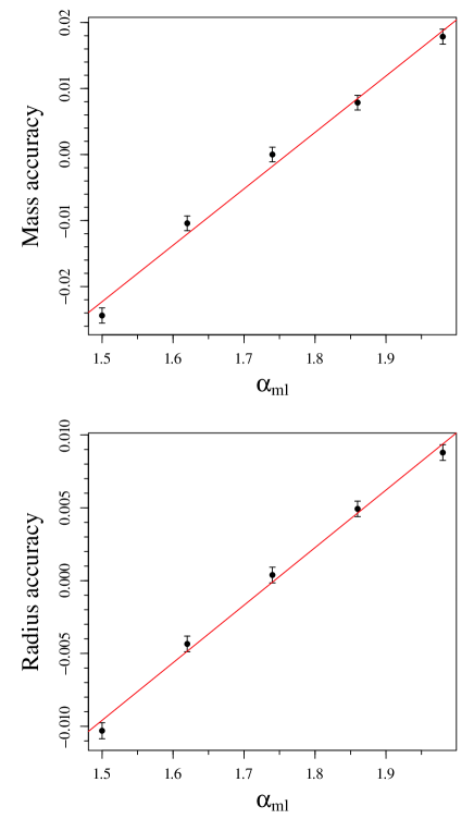
To establish the influence of varying the super-adiabatic convective transport efficiency, we computed four additional grids of stellar models by assuming mixing-length parameters that are different from the solar-calibrated one: $\alpha_{\rm ml}$ = 1.50, 1.62 1.86, and 1.98. Then, we built four different synthetic datasets of artificial stars by sampling $N=10000$ stars for each of the four supplementary non-standard grids with different values of the mixing-length parameter. Then we applied our recovery procedure, based on the standard grid of stellar models, on these datasets in order to estimate the stellar masses and radii. The comparison between recovered and true values allows the effect of a variation in the mixing-length parameter to be quantified.

The results are shown in rows 4-7 of Table 1 and in Fig. 7 for both mass and radius estimates. The extreme change in $\alpha_{\rm ml}$ (i.e. $\pm 0.24$) induces a bias in mass and radius estimates of about $\pm 2.1\%$ and $\pm 1.0\%$, which is similar to the one caused by the $\Delta Y/\Delta Z$ variation discussed in Sect. 5.1. Figure 7 shows the dependence of the median of the relative errors distribution on the $\alpha_{\rm ml}$ adopted in the sampling grids. The trend is nearly linear, although the fit is not as good as in the other cases discussed in this work. As for initial helium abundance variation, the bias is dominated by the statistical errors.

As expected, the synthetic datasets sampled from the models with higher (lower) values of $\alpha_{\rm ml}$ are reconstructed with higher (lower) masses. In fact a higher value of $\alpha_{\rm ml}$ results in MS synthetic stars with higher effective temperature, which mimic more massive objects with standard $\alpha_{\rm ml}$.

Figure 7: As in Fig. 5, but for synthetic data sampled from grids with different $\alpha_{\rm ml}$ values and reconstructed with the standard grid for $\alpha_{\rm ml}=1.74$.

Figures 8 and 9 display, for $\alpha_{\rm ml}$ = 1.50 and 1.98 respectively, the same quantities of Fig. 2. A comparison of the two figures shows the different trend in the mass relative error vs. relative age plots. In detail, for $\alpha_{\rm ml}=1.98$, the spread of the relative errors in the estimated mass is lower at low values of relative ages. The mass is generally overestimated at high relative ages. For $\alpha_{\rm ml}=1.50$ instead, the variance of the relative errors is almost constant, and the mass is underestimated; in the last 20% of the relative age, the underestimation is smaller than in the first part of the plot. All these trends are edge effects similar to the ones described in Sect. 4, and they are the responsible for the deviation from the linear relation visible in Fig. 7. The importance of this distortion is greatest for $\alpha_{\rm ml}=1.98$. Restricted to relative ages greater than 0.35, hence avoiding the strong edge effect present in this case, the median of the mass relative error increases from 1.79% (Row 7 in Table 1) to 2.13%, which is nearly symmetrical to the value $-2.44\%$ obtained for $\alpha_{\rm ml}=1.50$ (Row 4 in Table 1).

The effect of sampling from grids computed with different values of mixing-length has been previously investigated in Basu et al. (2012), but with a different approach. In that work the synthetic grid consisted on a pool of nine sub-grids with $\alpha_{\rm ml}$ from 1.5 to 2.4 (their solar calibrated value being 1.826). In that paper three different sets of uncertainty on the observational quantities are considered; we report here the results for the Error 2 set (in their Table 1), i.e. 1.0% in $\Delta\nu$, 2.5% in $\nu_{\rm max}$, 100 K in $T_{\rm eff}$, and 0.25 dex in [Fe/H]. The bias resulting from the reconstruction of the sampled objects – in the seismic case – is 3.50% in mass and 1.32% in radius with spreads of 6.86% and 2.64%, respectively. Since the sampling procedure is different, these results cannot be directly compared with ours. In fact, the results presented in Rows 4-7 of Table 1 are computed by adopting a unique value of $\alpha_{\rm ml}$ in the synthetic grid. It is expected that the sampling from a pool of grids with $\alpha_{\rm ml}$ symmetric around the solar-scaled value result in negligible bias, except for a small distortion due to edge effects. The variance is expected to be inflated since it will also account for the difference in the mean of the estimates obtained from the different grids in the pool.

Figure 8: As in Fig. 2, but for synthetic data sampled from a grid with $\alpha_{\rm ml}=1.50$, and estimated with the standard grid (i.e. $\alpha_{\rm ml}=1.74$).

Figure 9: As in Fig. 2, but for synthetic data sampled from a grid with $\alpha_{\rm ml}=1.98$ and estimated with the standard grid (i.e. $\alpha_{\rm ml}=1.74$).

5.3 Radiative opacity, ¹⁴N$(p,\gamma)^{15}$O rate, and diffusion velocity

Even in the ideal case in which the metallicity, the helium abundance, and the mixing-length parameter were exactly known, the resulting stellar models would still be affected by a non-negligible uncertainty owing to the current degree of knowledge of the input physics required to solve stellar evolution equations. In Valle et al. (2013a, b), we devoted a strong computational effort to try to quantify the cumulative uncertainty affecting stellar models due to the combined effect of the main input physics (radiative opacity, nuclear reaction cross sections, etc.), focussing in particular on some relevant evolutionary features.

However, the effect of these uncertainties on the stellar parameters estimated by means of grid-based techniques has never been investigated. This section represents the first attempt to fill such a gap.

To quantify the impact of the current uncertainties on the microphysics, we computed additional grids of models by adopting perturbed input physics. Relying on the results of our previous papers, we can limit the analysis only to the three input shown to be relevant in the evolutionary stages and mass range studied here, i.e. the radiative opacities, the ¹⁴N$(p,\gamma)^{15}$O reaction rate, and the microscopic diffusion velocities. In light of the results presented in Valle et al. (2013a, b), the impact of the radiative opacity is expected to dominate the others. As discussed in detail in that paper, we assume an uncertainty of 5% in radiative opacities, of 15% in microscopic diffusion velocities, and of 10% in the ¹⁴N$(p,\gamma)^{15}$O reaction rate. As shown in our previous work, as far as perturbations of the input physics of these order are considered, the interactions among them can be neglected. Therefore, we computed grids by changing one input at the time while keeping all the others fixed to the standard values.

In more detail, we computed two grids assuming, respectively, high and low values of radiative opacities (i.e. $k_{\rm r}\pm$ 5%), two grids with high and low values of microscopic diffusion velocities (i.e. $v_{\rm d}\pm$ 15%), and two with high and low values of the ¹⁴N$(p,\gamma)^{15}$O reaction rate (i.e. $\sigma\pm$ 10%).

To assess the importance of these uncertainties, we built synthetic datasets of artificial stars by sampling $N=10000$ objects from each of these six non-standard grids. Then we applied our recovery procedure based on the standard grid of stellar models on these datasets in order to estimate the masses and radii. The comparison between recovered and true values allows the effect of the current uncertainty in the input physics adopted in stellar evolution codes to be quantified. The results are summarized in the Rows 8-13 of Table 1. Fig. 10 displays the same quantities of Fig. 2 for the only relevant case, the one with $k_{\rm r}\pm$ 5%. In fact, only the radiative opacity perturbation produces a relevant effect on the mass estimates (see e.g. Fig. 10). For radius estimates the microscopic diffusion velocities perturbation has an effect of about one half of the one from the opacity variation. In all the cases the statistical errors dominate over the bias.

The recovery procedure applied to the two synthetic datasets obtained by adopting perturbed values of radiative opacity ($k_{\rm r}\pm 5\%$) produces a bias in mass relative error of about $\mp 1.0\%$ and of about $\mp 0.45\%$ in radius relative errors. As shown in Fig. 10, the effects are symmetric with respect to the standard value, which corresponds to the case discussed in Sect. 5. These effects are about one half of those due to the initial helium abundance uncertainty and the extreme mixing-length variation analysed in this work. The trend of the median of the relative errors distribution with the opacity perturbation can be understood by considering that a lower value of radiative opacity will result in hotter artificial stars, which mimic more massive stellar models computed with standard opacity.

Figure 10: As in Fig. 5, but for synthetic data sampled from grids with different values of radiative opacity and reconstructed with the standard grid.

Figure 11: As in Fig. 2, but for synthetic data sampled from a grid with $k_{\rm r}$ at its low value, estimated on the standard grid.

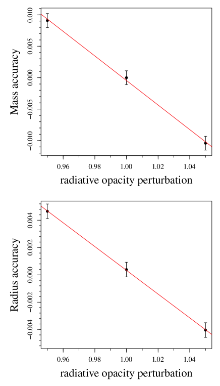
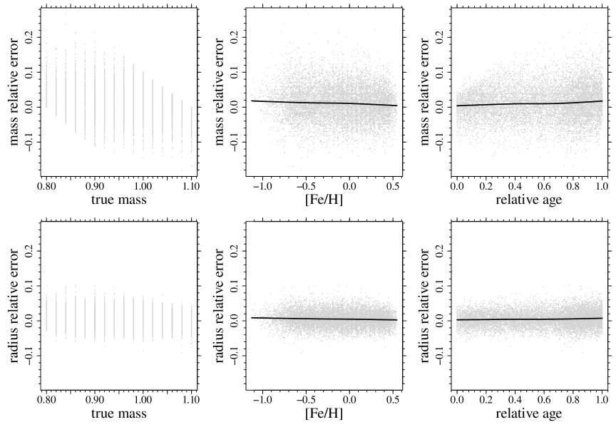
Figure 11 displays the dependence of relative errors on the mass and radius on the true mass of the stars, on [Fe/H], and on the relative age of the star. We observe that the performance of the grid-based estimates does not depend on the metallicity, and the dependence on stellar relative age shows a signature of the edge effect, as in the cases discussed above.

5.4 Cumulative effect of mixing-length, helium abundance, and radiative opacity uncertainties

The possible interactions between simultaneous variations in the mixing-length parameter and initial helium content or radiative opacity can, in principle, result in biases in mass and radius estimates that are not the simple sum of the biases due to the single input.

To test this hypothesis, we computed four further non-standard grids of stellar models by simultaneously varying two different inputs in order to explore possible interactions. The first two grids are calculated by combining the variations in initial helium content and mixing-length parameter: the former with $\Delta Y/\Delta Z=1$ and $\alpha_{\rm ml}=1.50$, the latter with $\Delta Y/\Delta Z=3$ and $\alpha_{\rm ml}=1.98$. The other two grids take the variation in mixing-length and radiative opacities simultaneously into account: the former adopting $\alpha_{\rm ml}=1.98$ and low values of radiative opacities, the latter with $\alpha_{\rm ml}=1.50$ and high values of radiative opacities. These cases correspond to the maximum variation expected by crossing the selected inputs. Then, we built synthetic datasets of artificial stars by sampling $N=10000$ objects from each of these four non-standard grids of stellar models. The mass and radius of the objects are finally estimated using the recovery procedure based on the standard grid.

The results are summarized in Rows 14-17 of Table 1. In all four cases, the bias of mass and radius estimates are consistent with the sum of the single biases illustrated in the previous sections. In these cases the statistical errors are nearly the same as the systematic ones. This implies that the cumulative uncertainty in the model calculations can result in significantly distorted estimates of stellar characteristics.

6 Effects of neglecting element diffusion in the stellar model grid

The surface [Fe/H] value observed in real low-mass MS stars clearly represents the abundance currently present in the atmosphere. Such an abundance can be quite different from the initial one, depending on the stellar age and mass, owing to the microscopic diffusion processes.

Figure 12 shows the [Fe/H] evolution for two stars of $M$ = 0.8 and 1.00 $M_{\sun}$ with three different initial metallicities ([Fe/H] = $-0.55$, 0.00, 0.55). The general trend is that, during the central hydrogen burning, the surface [Fe/H] drops from the ZAMS value and reaches a minimum at about 90% of its evolution before central hydrogen exhaustion. After this point it starts to increase again because of the sink of the convective envelope, which reaches more internal regions where metals were previously accumulated by gravitational settling. The amount of the decrease depends on the mass and initial metallicity of the star. The lower the initial metallicity, the higher the drop due to the reduced extension of the external convective region, which inhibits diffusion. The surface [Fe/H] decrease is around 0.1-0.15 dex, with the exception of the 1.0 $M_{\sun}$ model with initial [Fe/H] = $-0.55,$ which shows a dramatic iron depletion (i.e. about 0.55 dex) due to the vanishing convective envelope.

Figure 12: Evolution of surface [Fe/H] for two different masses $M$ = 0.80 and 1.00 $M_{\sun}$ (identified by the black circle and red triangle, respectively) and initial [Fe/H] = $-0.55$, 0.00, and 0.55.

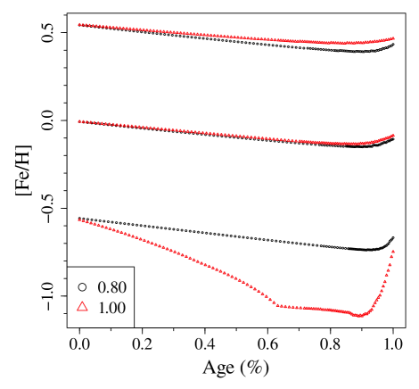
These effects of the microscopic diffusion must be taken into account whenever the stellar parameters of low-mass MS stars have to be determined, since neglecting them and using the initial [Fe/H] in the estimation grid would introduce a systematic bias.

Nevertheless, some widely used stellar model grids in the literature, namely BaSTI (Pietrinferni et al. 2004, 2006) and STEV (Bertelli et al. 2008, 2009) do not implement diffusion. The same occurs in stellar models used in some grid-based technique, such as RADIUS (Stello et al. 2009) and SEEK, which both adopt a grid of models computed with the Aarhus STellar Evolution Code (Christensen-Dalsgaard 2008).

Thus, it is useful to analyse the distortion in grid-based estimates that arises whenever the effects of the diffusion are neglected. To do this, we follow a different approach to the cases discussed above, where the recovery procedure has always been performed by means of the same standard estimation grid of models, and the various sources of uncertainty were taken into account in the synthetic dataset construction. In contrast, we think that is more realistic in this case to build the artificial stars by sampling from the standard grid of models, which takes the element diffusion into account, as in real stars, and to use non-standard models for the recovery.

Since diffusion affects not only the surface chemical abundance but also the internal structure and evolution of low-mass MS stars, we study two different cases. In the first one, the estimation grid stellar models have been computed without element diffusion, whereas in the second one diffusion is allowed, but the surface evolution of [Fe/H] is neglected in the recovery procedure (i.e. the [Fe/H] value in the evolutionary tracks is fixed to be equal to its initial value). In the latter case, the effect on the reconstructed mass and radius is only due to an incorrect initial metallicity evaluation, since one would assign an initial metal abundance equal to the observed surface one to the observed star, thus underestimating the metallicity. In the former, one would also neglect the other evolutionary effects of diffusion.

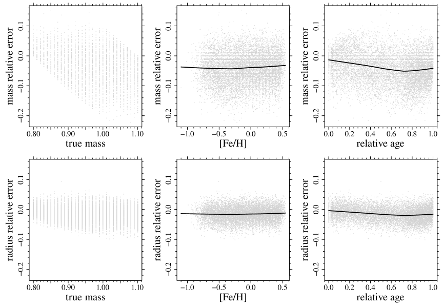
The results of the first case, i.e. completely neglecting the diffusion in the estimation grid, are summarized in Rows 18 of Table 1. The bias in mass relative error is about $-3.7\%$, while it is about $-1.5\%$ for radius relative errors. The statistical errors, about $5.0\%$ and $2.3\%$ respectively, are very close to the biases. The biases turn out to be comparable to the one presented in Row 17 of Table 1, obtained for the combined variation of mixing-length parameter and radiative opacity. Figure 13 shows the dependence of relative errors in the mass and radius on the true mass of the stars, on [Fe/H], and on the relative age of the star. As expected, the effect of microscopic diffusion is greater at higher relative ages, since the timescale of the microscopic diffusion is a few Gyr. As a consequence the bias in the mass and radius estimates is greater for stars in late central hydrogen burning. Figure 13 also shows that around [Fe/H] = $-0.5,$ the underestimation of mass and radius is more than for metal-richer stars. This effect is the due to the metallicity dependence of the external convection extension, which inhibits diffusion, hence of the diffusion efficiency.

Figure 13: As in Fig. 2, but for synthetic data sampled from the standard grid and recovered on the grid, which does not include diffusion in the computations.

The results of the second case are summarized in Row 19 of Table 1. The bias in mass relative error is about $-2.6\%$, while it is about $-1\%$ for radius relative errors. The statistical errors, about $4.8\%$ and $2.3\%$ respectively, are dominant in both cases.

As one can see in Row 2 of Table 1, these values are nearly the same as those due to the initial helium abundance uncertainty. From Fig. 14, it appears that the trend of the relative errors in mass and radius are similar to those discussed above that result from the complete neglecting of diffusion.

The comparison of the results reported in Rows 18 and 19 in Table 1 shows that the neglecting of surface [Fe/H] evolution is the main bias source, since it accounts for about two-thirds of the overall bias due to completely neglecting diffusion in stellar evolution.

Figure 14: As in Fig. 2, but for synthetic data sampled from the standard grid and recovered on the same grid but whithout taking the surface [Fe/H] evolution into account.

7 Possible extensions of the standard estimation grid

An extension of the estimation grid with models computed with different input physics and parameters might in principle improve mass and radius estimates in the presence of unknown sources of uncertainty. The general idea is that the presence of grids computed with different mixing-length values or different radiative opacities can mimic the variation induced by other sources of uncertainty, e.g. the initial helium contents. As a result the additional grids would help to keep the hidden variability under control, providing less biased estimates. A similar method has already been adopted in the literature (see e.g. Basu et al. 2012), although with some differences to the computations presented here.

To check such a working hypothesis, we built synthetic datasets of artificial stars by sampling from a grid of models not included in the estimation process. In other words, we did not sample the synthetic stars from the same grids used in the recovery procedure, unlike Basu et al. (2012). This is a subtle but important distinction. If the synthetic dataset were built from the same extended grid of models as used for the subsequent recovery procedure, the resulting estimates would by necessity be less biased than the ones obtained from the standard grid alone, since in this case the extended grid indeed also contains the sampled synthetic stars. This is clearly not the case when synthetic stars are sampled from grids that are not included.

To assess the usefulness of the grid extension we adopted the following approach. As a first test, we built two synthetic datasets of artificial stars by sampling $N=10000$ objects from non-standard grids of stellar models with mixing-length values different from the solar calibrated one, namely $\alpha_{\rm ml}$ = 1.50 and 1.98. Then we applied the recovery procedure to estimating the mass and radius of these objects and added all the stellar models computed with different values of initial helium abundance to our standard estimation grid (i.e. $\Delta Y/\Delta Z$ = 1 and 3). The results are summarized in Rows 1 and 2 of Table 3.

As a second test, we built two other synthetic datasets of artificial stars by sampling $N=10000$ objects from the non-standard grids of stellar models computed with high and low radiative opacities values. Then we reconstructed the mass and radius by adopting the same extended grid used in the previous test in the recovery procedure (results in Rows 3-4 of Table 3).

Finally, we analysed the same synthetic dataset as for the first test (i.e. non-solar mixing-length parameters) but adopted a different extended grid that includes the two non-standard grids computed with high and low radiative opacities beyond the standard one (results in Rows 5-6 of Table 3).

The comparison of the results reported in Table 3 (Rows 1-4) with those presented in Table 1 (Rows 4, 7, 8, 9) shows that the insertion of non-standard grids computed with different $\Delta Y/\Delta Z$ values produces estimates of mass and radius with a slightly reduced bias, but at the expense of an increase in the statistical error by about 15%. The estimates obtained from the grid that includes non-standard models with different values of the radiative opacity (Rows 5-6 in Table 3) do not differ significantly from the ones obtained with the standard grid only (Rows 4 and 7 in Table 1).

The importance of a multi-mixing-length recovery grid can be different for different stellar evolutionary stages or for different sources of uncertainty. As an example, in Basu et al. (2012) – which considers stars up to 3.0 $M_{\sun}$, including the red giant phase – it was stated that, for stars sampled from a grid computed with different boundary conditions, the bias of the mass estimates is lower in the multi-grid case.

Table 1: Summary of mass and radius relative errors.

	Label	Median	95% CI	Std. dev.	95% CI	$q_{16}$	$q_{84}$
Mass estimate
1	standard	0.0000	0.0011	0.0450	0.0006	-0.043	0.042
2	$\Delta Y/\Delta Z$ = 1	-0.0244	0.0012	0.0487	0.0007	-0.075	0.017
3	$\Delta Y/\Delta Z$ = 3	0.0227	0.0012	0.0490	0.0007	-0.019	0.075
4	$\alpha_{\rm ml}$ = 1.50	-0.0244	0.0011	0.0468	0.0006	-0.074	0.016
5	$\alpha_{\rm ml}$ = 1.62	-0.0104	0.0011	0.0454	0.0006	-0.058	0.029
6	$\alpha_{\rm ml}$ = 1.86	0.0079	0.0011	0.0455	0.0006	-0.031	0.054
7	$\alpha_{\rm ml}$ = 1.98	0.0179	0.0011	0.0463	0.0006	-0.020	0.067
8	$k_{\rm r}$ low	0.0091	0.0011	0.0453	0.0006	-0.030	0.055
9	$k_{\rm r}$ high	-0.0104	0.0011	0.0446	0.0006	-0.055	0.028
10	14N$(p,\gamma)^{15}$O low	0.0000	0.0011	0.0451	0.0006	-0.044	0.041
11	14N$(p,\gamma)^{15}$O high	0.0000	0.0011	0.0444	0.0006	-0.044	0.040
12	$v_{\rm d}$ low	0.0000	0.0011	0.0454	0.0006	-0.038	0.048
13	$v_{\rm d}$ high	-0.0027	0.0011	0.0447	0.0006	-0.048	0.038
14	$\alpha_{\rm ml}$ = 1.50, $\Delta Y/\Delta Z$ = 1	-0.0476	0.0013	0.0515	0.0007	-0.104	0.000
15	$\alpha_{\rm ml}$ = 1.98, $\Delta Y/\Delta Z$ = 3	0.0395	0.0013	0.0514	0.0007	0.000	0.100
16	$\alpha_{\rm ml}$ = 1.98, $k_{\rm r}$ low	0.0284	0.0011	0.0463	0.0006	-0.009	0.078
17	$\alpha_{\rm ml}$ = 1.50, $k_{\rm r}$ high	-0.0365	0.0011	0.0465	0.0006	-0.085	0.003
18	no diffusion	-0.0370	0.0012	0.0496	0.0007	-0.091	0.008
19	no [Fe/H] evolution	-0.0257	0.0012	0.0481	0.0007	-0.076	0.014
Radius estimate
1	standard	0.0004	0.0005	0.0219	0.0003	-0.021	0.022
2	$\Delta Y/\Delta Z$ = 1	-0.0106	0.0006	0.0235	0.0003	-0.033	0.013
3	$\Delta Y/\Delta Z$ = 3	0.0109	0.0006	0.0233	0.0003	-0.012	0.034
4	$\alpha_{\rm ml}$ = 1.50	-0.0103	0.0005	0.0222	0.0003	-0.032	0.012
5	$\alpha_{\rm ml}$ = 1.62	-0.0043	0.0005	0.0219	0.0003	-0.026	0.017
6	$\alpha_{\rm ml}$ = 1.86	0.0049	0.0005	0.0219	0.0003	-0.016	0.027
7	$\alpha_{\rm ml}$ = 1.98	0.0088	0.0005	0.0219	0.0003	-0.012	0.031
8	$k_{\rm r}$ low	0.0047	0.0005	0.0219	0.0003	-0.016	0.027
9	$k_{\rm r}$ high	-0.0040	0.0005	0.0219	0.0003	-0.025	0.017
10	14N$(p,\gamma)^{15}$O low	0.0003	0.0005	0.0223	0.0003	-0.021	0.022
11	14N$(p,\gamma)^{15}$O high	-0.0002	0.0005	0.0215	0.0003	-0.020	0.022
12	$v_{\rm d}$ low	0.0021	0.0005	0.0218	0.0003	-0.018	0.024
13	$v_{\rm d}$ high	-0.0015	0.0005	0.0218	0.0003	-0.022	0.020
14	$\alpha_{\rm ml}$ = 1.50, $\Delta Y/\Delta Z$ = 1	-0.0199	0.0006	0.0244	0.0003	-0.044	0.004
15	$\alpha_{\rm ml}$ = 1.98, $\Delta Y/\Delta Z$ = 3	0.0187	0.0006	0.0239	0.0003	-0.004	0.044
16	$\alpha_{\rm ml}$ = 1.98, $k_{\rm r}$ low	0.0126	0.0005	0.0220	0.0003	-0.008	0.035
17	$\alpha_{\rm ml}$ = 1.50, $k_{\rm r}$ high	-0.0144	0.0005	0.0224	0.0003	-0.037	0.007
18	no diffusion	-0.0149	0.0006	0.0234	0.0003	-0.038	0.008
19	no [Fe/H] evolution	-0.0104	0.0006	0.0228	0.0003	-0.033	0.012

Table 2: Summary of standard deviation of mass and radius relative errors obtained adopting reduced errors on observation constraints. For the observables not explicitly indicated in the labels, the errors are the same as those adopted in the standard case.

	Label	std. dev.	$q_{16}$	$q_{84}$
Mass estimate
1	$\sigma(T_{\rm eff})=$ 50 K	0.0350	-0.034	0.031
2	$\sigma([Fe/H])=$ 0.05 dex	0.0392	-0.038	0.037
3	$\sigma(\Delta\nu)=$ 1%, $\sigma(\nu_{\rm max})=$ 2.5%	0.0427	-0.041	0.040
4	all the above	0.0246	-0.023	0.023
Radius estimate
1	$\sigma(T_{\rm eff})=$ 50 K	0.0193	-0.018	0.020
2	$\sigma([Fe/H])=$ 0.05 dex	0.0203	-0.019	0.020
3	$\sigma(\Delta\nu)=$ 1%, $\sigma(\nu_{\rm max})=$ 2.5%	0.0164	-0.016	0.016
4	all the above	0.0108	-0.010	0.011

Table 3: Summary of mass and radius relative errors obtained adopting non-standard estimation grid.

	Label	Estimation grid	Median	95% CI	Std. dev.	95% CI	$q_{16}$	$q_{84}$
Mass estimate
1	$\alpha_{\rm ml}$ = 1.50	std. + He	-0.0208	0.0014	0.0552	0.0008	-0.080	0.028
2	$\alpha_{\rm ml}$ = 1.98	std. + He	0.0111	0.0013	0.0533	0.0007	-0.032	0.070
3	$k_{\rm r}$ low	std. + He	0.0062	0.0013	0.0529	0.0007	-0.041	0.060
4	$k_{\rm r}$ high	std. + He	-0.0096	0.0013	0.0533	0.0007	-0.062	0.038
5	$\alpha_{\rm ml}$ = 1.50	std. + $k_{\rm r}$	-0.0244	0.0012	0.0470	0.0007	-0.073	0.019
6	$\alpha_{\rm ml}$ = 1.98	std. + $k_{\rm r}$	0.0160	0.0012	0.0472	0.0007	-0.024	0.066
Radius estimate
1	$\alpha_{\rm ml}$ = 1.50	std. + He	-0.0081	0.0006	0.0253	0.0004	-0.034	0.016
2	$\alpha_{\rm ml}$ = 1.98	std. + He	0.0067	0.0006	0.0244	0.0003	-0.016	0.032
3	$k_{\rm r}$ low	std. + He	0.0040	0.0006	0.0243	0.0003	-0.019	0.028
4	$k_{\rm r}$ high	std. + He	-0.0042	0.0006	0.0246	0.0003	-0.028	0.021
5	$\alpha_{\rm ml}$ = 1.50	std. + $k_{\rm r}$	-0.0098	0.0005	0.0224	0.0003	-0.032	0.012
6	$\alpha_{\rm ml}$ = 1.98	std. + $k_{\rm r}$	0.0085	0.0005	0.0224	0.0003	-0.013	0.031

8 Comparison with other techniques

Computation of the bias on the estimated mass and radius presented in the previous sections shed some light on the magnitude of systematic errors due to some uncertainties affecting stellar evolution. These computations have been obtained using a single evolutionary code, so they share a large number of input physics and algorithmic approaches. The comparison with the results obtained by other authors on a common set of objects is therefore of high interest for estimating the possible contributions to the systematic uncertainty arising from different stellar evolutionary computations and from different recovery techniques.

In this section we apply our standard estimation grids to recovering stellar parameters of seven objects – K3656476, K6116048, K7976303, K8006161, K8379927, K10516096, and K10963065 – from the Kepler catalogue. The selected objects have been extensively studied by Mathur et al. (2012), along with other 15 objects that lie outside our estimation grid, by adopting RADIUS, YB, and SEEK.

The RADIUS method (Stello et al. 2009) uses $T_{\rm eff}$, $\log g$, [Fe/H], $L$, and $\Delta\nu$ to find the optimal model. It is based on a large grid of stellar models computed with the Aarhus STellar Evolution Code (Christensen-Dalsgaard 2008), which does not include rotation, overshooting, and diffusion. The grid has fixed values of the mixing-length and initial helium abundance at a given metallicity. The Grevesse & Noels (1993) solar mixture is adopted. The metallicity $Z$ is in the range [0.001 - 0.055], and the mass step is 0.01 $M_{\sun}$ in the range [0.5 - 4.0] $M_{\sun}$. The recovery technique identifies a $3\sigma$ region in the observation hyperspace around the object to reconstruct, finds the extreme values of mass and radius in this set, and reports their averages as mass and radius estimates.

The YB method uses a variant of the Yale-Birmingham code (Gai et al. 2011) and adopts the same estimation technique as in the present work. The recovery is based on the following observables: $T_{\rm eff}$, [Fe/H], $\Delta\nu$, and $\nu_{\rm max}$. The grid of stellar models is computed with the Yale rotating evolution code (Demarque et al. 2008) in its non-rotating configuration. The grid spans the mass range [0.80 - 3.0] $M_{\sun}$ in steps of 0.02 $M_{\sun}$. The metallicity [Fe/H] ranges from $-0.6$ to 0.6 dex, with solar abundance according to Grevesse & Sauval (1998). The initial helium abundance is linked to the metallicity assuming $\Delta Y/\Delta Z=1$.

The SEEK technique requires the use of a large grid of stellar models computed with the Aarhus Stellar Evolution Code (Christensen-Dalsgaard 2008), and it adopts a Bayesian approach in the estimation procedure. The grid is composed of 7300 evolution tracks with different mixing-length parameters and initial helium abundances at a given metallicity. It adopts the solar mixture of Grevesse & Sauval (1998). The mass step in the range [0.6 - 1.8] $M_{\sun}$ is 0.02 $M_{\sun}$. The metallicity range of the grid is $Z$ $\in$ [0.005, 0.03]. The observables used in the reconstruction are $T_{\rm eff}$, [Fe/H], and $\Delta\nu$.

Table 4 lists the observational constraints adopted in the estimation. Regarding the seismic quantities, we adopt a slightly conservative approach – which accounts for the uncertainty in the solar seismic values – and we assume a common uncertainty of 1% in $\Delta\nu$ and 5% in $\nu_{\rm max}$.

In Table 6 we present the results of the estimation procedure. The table lists the results obtained using only the standard grid and those obtained also using the grids of stellar models with different mixing-length values and different initial helium contents. The second approach is similar to the one adopted in the SEEK technique. The corresponding estimates quoted in Mathur et al. (2012) are in Table 7. As noted in Sect. 7, the statistical error from the multi-grid estimation technique is often larger than the one from the single-grid technique. This effect can be anticipated since the estimates in the multi-grid cases can be viewed as the pool of the estimates obtained on the different grids inserted in the recovery procedure. All these estimates have almost equal variance (see Table 1). The total variance of the mass and radius estimates are then slightly inflated by the presence of the systematic bias of the estimates on the different grids in the recovery procedure. This small amount of inflaction confirms that the statistical component of the error term is more important than the systematic shift in the estimates due to the differences in the grids. Obviously, an improvement on the precision of the stellar observables will modify the balance of these two error terms, since the statistical errors will shrink (see e.g. Gai et al. 2011).

Although the adopted technique is the same as YB, the results of the present work match those provided by the SEEK technique best. In fact in all the studied cases, our and SEEK estimates of both mass and radius are consistent within the errors. This results illustrates the difficulties in disentangling the various input and techniques adopted in the grid estimation procedure. The SEEK grid does not include microscopic diffusion, which is shown here to contribute largely to biasing the estimates of mass and radius, but this bias is cancelled out by the other differences in the evolutionary code and in the estimation technique.

Comparison with the estimates obtained by YB is highly informative since it highlights the systematic uncertainty arising only from the differences in the stellar evolution computations, because the recovery procedure is the same. The YB mass estimates of K6116048 and K8379927 are significantly higher – at $1\sigma$ level – than the ones obtained here using the standard reconstruction grid, but consistent with the estimates obtained using all the other grids. As for radii, YB estimates for K6116048, K7976303, and K8379927, are significantly larger than the ones obtained here, while for K10516096 the estimate is significantly lower.

A general agreement among the estimation techniques is not unexpected. In fact, we are focussing on central hydrogen burning stars in a narrow range of masses around the solar one. In these cases, the common procedure of calibrating the mixing-length parameter to the Sun will keep most of the differences induced by the different input physics in the evolutionary codes under control. A poorer agreement is expected whenever later stages, e.g. the red giant branch evolution, are considered. Nevertheless, even from the analysis of the few objects presented here, we note that the differences in the assumptions made in the different codes (input physics, convection and diffusion efficiencies, chemical composition, etc.) play a fundamental role. The mass estimates provided by all of the techniques agree within the errors only for K7976303, K8006161, K10516096, and K10963065, while the agreement of both mass and radius is only obtained for K10963065.

A simple exercise gives an idea of the range of mass spanned by the different estimation techniques. We averaged the differences in the higher and lower estimates obtained by the four techniques for all the seven objects. The result is $\left<\Delta M\right>=0.14$ $M_{\sun}$, which is much higher than the statistical components of the error obtained by the grid techniques. As a reference, the mean of these latter errors is about 0.05 $M_{\sun}$. The same computation performed on radii gives an average of $\left<\Delta R\right>=0.11$ $R_{\sun}$; even in this case, the systematic error is more than the statistical ones (the mean of statistical errors is about 0.02 $R_{\sun}$).

It is apparent that the magnitude of the systematic error shown here is much larger than the one reported in the analyses of the previous sections and that it is dominant over the statistical component. It appears that the differences in the evolutionary codes and in the recovery techniques play a fundamental role in estimating stellar parameters. Since the refinement of the observation techniques will make data available with increasing precision, it is expected that this conclusion will strengthen in the near future, since better observation precision will obviously lead to smaller statistical errors, as displayed in Table 2 (see also Gai et al. 2011).

As a final remark, the asteroseismic radius of KIC 8006161 has been verified using parallaxes (Silva Aguirre et al. 2012) and interferometry (Huber et al. 2012). The values are $R=0.927\pm 0.014$ $R_{\sun}$ and $R=0.952\pm 0.021$ $R_{\sun,}$ respectively. The results reported here ($R=0.92\pm 0.01$ $R_{\sun}$ for single grid estimate, and $R=0.93\pm 0.02$ $R_{\sun}$ for multi-grid estimate) agree with these determinations.

Table 4: Observational sample of stars from the Kepler catalog selected for the estimation procedure.

Star	$T_{\rm eff}$ (K)	[Fe/H]	$\Delta\nu$ ($\mu$Hz)	$\nu_{\rm max}$ ($\mu$Hz)
K3656476	5700 $\pm$ 70	0.32 $\pm$ 0.07	93.70 $\pm$ 0.22	1940 $\pm$ 25
K6116048	5895 $\pm$ 70	-0.26 $\pm$ 0.07	100.14 $\pm$ 0.22	2120 $\pm$ 20
K7976303	6050 $\pm$ 70	0.10 $\pm$ 0.07	50.95 $\pm$ 0.37	910 $\pm$ 25
K8006161	5340 $\pm$ 70	0.38 $\pm$ 0.07	148.21 $\pm$ 0.19	3545 $\pm$ 140
K8379927	5960 $\pm$ 125	-0.30 $\pm$ 0.12	120.86 $\pm$ 0.43	2880 $\pm$ 65
K10516096	5900 $\pm$ 70	-0.10 $\pm$ 0.07	84.15 $\pm$ 0.36	1710 $\pm$ 15
K10963065	6015 $\pm$ 70	-0.21 $\pm$ 0.07	103.61 $\pm$ 0.41	2160 $\pm$ 35

Observational data: Mathur et al. (2012).

Table 5: Observational sample of binary stars selected for the estimation procedure.

Star	$T_{\rm eff}$ (K)	[Fe/H]	$\Delta\nu$ ($\mu$Hz)	$\nu_{\rm max}$ ($\mu$Hz)	$M$ ($M_{\sun}$)	$R$ ($R_{\sun}$)	References
$\alpha$ Cen A	5847 $\pm$ 27	0.24 $\pm$ 0.03	105.5 $\pm$ 0.5	2410	1.105 $\pm$ 0.007	1.224 $\pm$ 0.003	1, a, A
$\alpha$ Cen B	5316 $\pm$ 28	0.25 $\pm$ 0.04	161.5 $\pm$ 0.5	4100	0.935 $\pm$ 0.006	0.863 $\pm$ 0.005	2, a, A
70 Oph A	5300 $\pm$ 50	0.04 $\pm$ 0.05	161.7 $\pm$ 0.8	4500	0.890 $\pm$ 0.020	–	3, b, B

Asteroseismology data: (1) Bouchy & Carrier (2002); (2) Kjeldsen et al. (2005); (3) Carrier & Eggenberger (2006). Other observables: (a) Porto de Mello et al. (2008); (b) Eggenberger et al. (2008). Masses and radii values: (A) Miglio & Montalbán (2005); (B) Eggenberger et al. (2008).

Table 6: Mass and radius estimates for the observational sample of Tables 4 and 5.

	Standard grid		Multi grids
Star	$M$ ($M_{\sun}$)	$R$ ($R_{\sun}$)	$M$ ($M_{\sun}$)	$R$ ($R_{\sun}$)
K3656476	1.06${}^{+0.03}_{-0.04}$	1.30${}^{+0.01}_{-0.02}$	1.08${}^{+0.02}_{-0.08}$	1.30${}^{+0.01}_{-0.03}$
K6116048	0.92 $\pm$ 0.04	1.19 $\pm$ 0.02	0.96 $\pm$ 0.04	1.20 $\pm$ 0.02
K7976303	1.06${}^{+0.02}_{-0.04}$	1.94 $\pm$ 0.02	1.08${}^{+0.04}_{-0.02}$	1.95${}^{+0.03}_{-0.02}$
K8006161	0.95 $\pm$ 0.03	0.92 $\pm$ 0.01	0.96${}^{+0.08}_{-0.06}$	0.93 $\pm$ 0.02
K8379927	0.96${}^{+0.02}_{-0.03}$	1.05 $\pm$ 0.02	0.99 $\pm$ 0.06	1.07 $\pm$ 0.02
K10516096	1.01 $\pm$ 0.04	1.37 $\pm$ 0.02	1.05${}^{+0.05}_{-0.04}$	1.39 $\pm$ 0.02
K10963065	0.98 $\pm$ 0.04	1.18 $\pm$ 0.02	1.00${}^{+0.04}_{-0.05}$	1.19 $\pm$ 0.02
$\alpha$ Cen A	1.09${}^{+0.01}_{-0.02}$	1.21 $\pm$ 0.01	1.10-0.02	1.21 $\pm$ 0.01
$\alpha$ Cen B	0.92${}^{+0.02}_{-0.01}$	0.86 $\pm$ 0.01	0.95${}^{+0.03}_{-0.04}$	0.87 $\pm$ 0.01
70 Oph A	0.86 $\pm$ 0.02	0.84 $\pm$ 0.01	0.90${}^{+0.02}_{-0.04}$	0.85 $\pm$ 0.01

Table 7: Mass and radius estimates from literature with different methods.

	RADIUS		YB		SEEK
Star	$M$ ($M_{\sun}$)	$R$ ($R_{\sun}$)	$M$ ($M_{\sun}$)	$R$ ($R_{\sun}$)	$M$ ($M_{\sun}$)	$R$ ($R_{\sun}$)	Ref.
K3656476	1.29 $\pm$ 0.06	1.38 $\pm$ 0.02	1.05 $\pm$ 0.04	1.28 $\pm$ 0.02	1.05${}^{+0.06}_{-0.03}$	1.32 $\pm$ 0.02	a
K6116048	0.86 $\pm$ 0.03	1.16 $\pm$ 0.01	1.03 $\pm$ 0.03	1.24${}^{+0.01}_{-0.02}$	0.93${}^{+0.07}_{-0.05}$	1.19${}^{+0.04}_{-0.03}$	a
K7976303	1.04 $\pm$ 0.03	1.93 $\pm$ 0.02	1.10${}^{+0.05}_{-0.08}$	2.07 ${}^{+0.05}_{-0.07}$	1.05${}^{+0.08}_{-0.04}$	1.98${}^{+0.03}_{-0.08}$	a
K8006161	1.07 $\pm$ 0.03	0.96 $\pm$ 0.01	0.96${}^{+0.08}_{-0.04}$	0.91 $\pm$ 0.01	1.00 $\pm$ 0.02	0.93 $\pm$ 0.02	a
K8379927	0.84 $\pm$ 0.03	1.01 $\pm$ 0.01	1.10 $\pm$ 0.06	1.13 $\pm$ 0.02	0.98${}^{+0.05}_{-0.08}$	1.06 $\pm$ 0.03	a
K10516096	1.00 $\pm$ 0.05	1.36 $\pm$ 0.03	1.02 $\pm$ 0.04	1.18 $\pm$ 0.03	1.05${}^{+0.10}_{-0.05}$	1.41 $\pm$ 0.03	a
K10963065	0.95 $\pm$ 0.04	1.17 $\pm$ 0.02	1.02${}^{+0.06}_{-0.07}$	1.19 $\pm$ 0.03	1.03${}^{+0.07}_{-0.05}$	1.21 $\pm$ 0.02	a
$\alpha$ Cen A					1.09 $\pm$ 0.09	1.23 $\pm$ 0.04	b
$\alpha$ Cen B					0.92 $\pm$ 0.04	0.87 $\pm$ 0.01	b
70 Oph A					0.89 $\pm$ 0.06	0.86 $\pm$ 0.02	b

9 Comparison with observations

Beyond the tests described in previous sections, any recovery procedure has to prove its performance against real data. A severe empirical test is provided by binaries stars for which precise mass and radius measurements are available.

We focus our attention on three binary stars for which independent estimates of mass and radius exist. The selected stars are $\alpha$ Cent A + B and 70 Oph A. These objects have recently been studied by Quirion et al. (2010) with the SEEK technique, so we can compare our results with both observations and SEEK estimates. The seismic and non-seismic observable quantities adopted in the estimation are listed in Table 5.

In Table 6 we present the results of the estimation procedure. This table lists the results obtained using the standard grid alone and those obtained also using the grids with different mixing-length and initial helium abundance values. The second approach is similar to the one adopted in the SEEK technique. In all the six cases the estimates of mass and radius reported in Table 6 are consistent within the errors.

The corresponding estimates obtained with the SEEK technique are in Table 7. It is apparent that the mass and radius obtained from the recovery grid are consistent with the values presented in Table 5.

10 Conclusions

In this work we investigated how the stellar model grid-based estimates of mass and radius of a star are influenced by systematic uncertainties arising from still uncertain knowledge of both the main input physics (radiative opacity, nuclear reaction cross sections, etc.) and macroscopic processes (superadiabatic convection, element diffusion, etc.) implemented in stellar codes.

To do that, we developed a code – SCEPtER (Stellar CharactEristics Pisa Estimation gRid), available on-line – to estimate stellar mass and radius through a grid-based maximum likelihood technique following Gai et al. (2011) and Basu et al. (2012). In the current version, we relied on four observable quantities, namely the effective temperature, the metallicity [Fe/H], the large frequency spacing $\Delta\nu$, and the frequency of maximum oscillation power $\nu_{\rm max}$ of the star. The grid of stellar models covers the evolutionary phases from ZAMS to the central hydrogen exhaustion in the mass range [0.8 - 1.1] $M_{\sun}$.

The present work focussed on estimating the statistical errors arising from the uncertainty in observational quantities and on estimating the systematic biases due to the uncertainties in initial helium content, in the mixing-length value, and in some input physics that enter into the stellar computations. For this last point, we focussed our attention on radiative opacities, on microscopic diffusion velocities, and on the ¹⁴N$(p,\gamma)^{15}$O reaction rate. These are the main sources of uncertainty in the considered evolutionary stages (see Valle et al. 2013a, b, for a detailed discussion). This is the first time that such an issue has been addressed.

We found that the statistical error component is almost the same for all the cases we studied. The standard deviations for mass and radius estimates are about 4.5% and 2.2%, even if the error on the single estimate can reach 20% and 10%, respectively.

The initial helium content adopted in the stellar computations is assumed to scale linearly with the metallicity $Z$. To model the uncertainty in its determination we adopted a reference slope of $\Delta Y/\Delta Z$ = 2 and studied the effect of choosing different slopes for the synthetic datasets, namely $\Delta Y/\Delta Z$ = 1 and 3. The systematic bias due to the variation in the initial helium content on the explored range is of the order of $\pm 2.3\%$ on mass and $\pm 1.1\%$ on radius, on average. However, for metal-rich stars (i.e. [Fe/H] $\geq$ 0.0) the effect gets as large as $\pm 4.8\%$ and $\pm 1.9\%$ for mass and radius estimates, becoming comparable with the statistical error.

The impact of the mixing-length value variation was studied by computing several synthetic grids with $\alpha_{\rm ml}$ from 1.50 to 1.98, with our solar calibrated value (i.e. $\alpha_{\rm ml}$ = 1.74) adopted as a reference for the recovery standard grid. We found that the bias induced by the extreme allowed variation is of the order of $\pm 2.1\%$ on mass and $\pm 1.0\%$ on radius.

The impacts of the uncertainties in input physics that enter into the stellar computations have been studied here for the first time. We found that the current uncertainty in radiative opacities – i.e. $\pm 5\%$ (Valle et al. 2013a) – accounts for a bias of about $\mp 1.0\%$ and $\mp 0.45\%$ in mass and radius determination, whereas the other explored uncertainty sources in the input physics only have a minor effect.

The combination of the biases of several sources of uncertainty showed that they can be directly added with no interaction effects. As an example, the bias due to the concomitant uncertainty in mixing-length and in initial helium content is about $\pm 4.3\%$ and $\pm 2.0\%$ in mass and radius determination, respectively. These values are very close to the statistical ones, implying that the estimates can be distorted in a non-negligible way.

Since several widely used databases of stellar models (e.g. Pietrinferni et al. 2004, 2006; Bertelli et al. 2008, 2009) and some grid-based technique, such as RADIUS (Stello et al. 2009) and SEEK, which both adopt a grid of models computed with the Aarhus STellar Evolution Code (Christensen-Dalsgaard 2008), do not implement diffusion, we considered the bias due to this neglect. We found that this bias is on average of about 3.7% and 1.5% on mass and radius determination. We also showed that the mass and radius estimated by relying on a grid of stellar models computed including microscopic diffusion, but neglecting the temporal evolution of the surface [Fe/H] in the recovery procedure, are affected by a bias of the order of two-thirds of what is produced by using stellar tracks without diffusion. In both cases, the bias is greater at later evolutionary phases and around [Fe/H] = $-0.5$.

These results show that the lack of precise knowledge about the physics of the star might result in biases that are in some cases of the same magnitude of the uncertainty arising from the observation errors. Since this last source of uncertainty is expected to shrink in the near future, owing to instrument improvements, the systematic bias will soon be the main source of uncertainty in the estimates provided by grid-based techniques. The halving of the observational errors with respect to those considered in the paper, a goal already reached for several stars, will decrease the statistical errors on mass and radius estimates at the level of their biases.

We compared the results obtained by the SCEPtER technique to those found with other grid-based techniques reported in the literature: RADIUS (Stello et al. 2009), YB (Gai et al. 2011), and SEEK (Christensen-Dalsgaard 2008). Selecting a homogeneous subset of seven targets from the Kepler catalogue, analysed in Mathur et al. (2012), we found that our estimates of mass and radius always agreed with those of the SEEK technique. Several disagreements were found in the comparisons with YB estimates, which are obtained with the same recovering technique used by us but with different stellar models grids. We found that the systematic differences among the estimates of the four techniques are from three to five times greater than the statistical errors of the estimates. This implies that the differences in the inputs of the stellar computations are at present the most important source of systematic biases on the mass and radius estimates obtained by grid-based methods.

Finally, we tested our recovery procedure against three binary stars for which mass and radius have been determined empirically. These systems have been studied by Quirion et al. (2010) with the SEEK technique. In all three cases our grid-based estimates of mass and radius agree with both the observations and the estimates obtained with the SEEK technique.

Appendix A Kernel density and LOWESS

The kernel density is a non-parametric estimate of the probability density function from a discrete set of data. It can be viewed as a generalization of the histogram, with better theoretical properties (Härdle & Simar 2012). For a set of $n$ observations $x_{1}$, $x_{2}$, $\ldots$, $x_{n},$ a kernel density with bandwidth $h$ has the form:

$$\hat{f}(x,h)=\frac{1}{nh}\sum_{i=1}^{n}K\left(\frac{x-x_{i}}{h}\right)$$ (7)

where the kernel function $K$ is chosen to be a probability density function. Several choices of kernel are available. In this work. we make use of a Gaussian kernel:

$$K(y)=\frac{1}{\sqrt{2\pi}}\exp\left(-\frac{y^{2}}{2}\right).$$ (8)

The kernel selection usually has a minor influence on the kernel estimate with respect to the bandwidth $h$. This parameter is selected balancing two effects since an increment of $h$ increases the bias of $\hat{f}$, while it reduces its variance. An often adopted choice for a Gaussian kernel is given by the rule of thumb (Silverman 1986):

$$\hat{h}=0.9\;{\rm min}(\hat{\sigma},R/1.34)\;n^{-1/5}$$ (9)

where $\hat{\sigma}$ is the sample standard deviation and $R$ the sample interquartile range.

Other choices for the bandwidth, based on the asymptotic expansion of the mean integrated squared error, are reported in the literature. The different choices have an impact on kernel estimator for multi-modal distributions, which is not the case of the present work. We refer interested readers to Feigelson & Babu (2012); Härdle & Simar (2012); Venables & Ripley (2002); Sheather & Jones (1991).

A frequently used bivariate smoother is the local regression technique LOWESS, which combines a linear least squares regression with a robust nonlinear regression. It provides a generally smooth curve, whose value at a particular location along the $x$ axis is only determined by the points in its neighbourhood. The first step is to fit a polynomial regression in a neighbourhood of $x$. A fraction $f$ of the $n$ sample points near $x$ is selected. We define $m=\lceil fn\rceil$ the number of points used in the fit. Then the technique obtains the estimates $\hat{\beta}$ by minimizing

$$\hat{y}=m^{-1}\sum_{i=1}^{m}W_{i}(x)\left(y_{i}-\sum_{j=0}^{p}\beta_{j}x_{j}\right)^{2}\;,$$ (10)

where $W_{i}(x)$ are the weights, usually obtained by the tricubic function:

$$W_{i}(x)=\left(1-\left|\frac{x-x_{i}}{d}\right|^{3}\right)^{3}\;,$$ (11)

where $d$ is the maximum distance between $x$ and the other predictor values $x_{i}$ in the span. For LOWESS estimates the value $p=1$ is usually adopted, implying a local linear regression. The model residuals $\hat{\epsilon}_{i}$ and the scale parameter $\hat{m}={\rm median}(\hat{\epsilon}_{i})$ are computed. The median absolute deviation $\hat{\sigma}$ of the residuals is evaluated: $\hat{\sigma}={\rm median}|\hat{\epsilon}_{i}-\hat{m}|$. Then the algorithm computes the robustness weights $\delta_{i}=R(\hat{\epsilon}_{i}/6\hat{\sigma})$, with $R(u)=15/16(1-u)^{2}$ for $|u|\leq 1$ and $R(u)=0$ otherwise. The local regression of Eq. (10) is computed again, but with weights given by $\delta_{i}K_{i}(x)$. This procedure is iterated a variable number of times between one and five; this makes the local estimate robust even in presence of outliers. Further details on the technique and on the numerical methods used to speed up the computations are available in Cleveland (1981).

The computations outlined in this section were performed using the functions density and lowess, available in the R 2.15.2 (R Development Core Team 2012).