Conservative effects in spin-transfer-driven magnetization dynamics

Abstract

It is shown that under appropriate conditions spin-transfer-driven magnetization dynamics in a single-domain nanomagnet is conservative in nature and admits a specific integral of motion, which is reduced to the usual magnetic energy when the spin current goes to zero. The existence of this conservation law is connected to the symmetry properties of the dynamics under simultaneous inversion of magnetisation and time. When one applies an external magnetic field parallel to the spin polarization, the dynamics is transformed from conservative into dissipative. More precisely, it is demonstrated that there exists a state function such that the field induces a monotone relaxation of this function toward its minima or maxima, depending on the field orientation. These results hold in the absence of intrinsic damping effects. When intrinsic damping is included in the description, a competition arises between field-induced and damping-induced relaxations, which leads to the appearance of limit cycles, that is, of magnetization self-oscillations.

The spin-transfer phenomenon and related spintronic applications have been the focus of considerable research in the past two decades Slonczewski (1996); Berger (1996); Tserkovnyak et al. (2005); Haney et al. (2008); Brataas et al. (2012). This research has been dominated by experimental and theoretical studies of spin-transfer-induced magnetization switching Katine et al. (2000); Bazaliy et al. (2004); Kubota et al. (2008); Liu et al. (2012), as well as spin-transfer-driven magnetization self-oscillations Kiselev et al. (2003); Rippard et al. (2004); Krivorotov et al. (2005); Bertotti et al. (2005, 2009). These studies have all been based on the seed idea that spin transfer manifests itself as a non-conservative torque that competes with intrinsic (thermal) damping. In particular, it has been realized that the mutual compensation of non-conservative effects caused by spin transfer and thermal damping is the physical mechanism for the formation of magnetization self-oscillations Slonczewski (1996); Bertotti et al. (2005); Li et al. (2005).

It is demonstrated in this Letter that in single-domain nanomagnets spin transfer may act as a purely conservative torque when electron spin polarization is directed along the intermediate (i. e., hard in-plane) anisotropy axis. Under these conditions, the following new physical features emerge: the appearance of purely conservative magnetization dynamics with closed precession-type trajectories; the existence of a special integral of motion for this conservative dynamics, which is reduced to the conventional magnetic energy at zero spin current; a very unique global bifurcation in magnetization dynamics occurring at a specific critical value of the injected spin-polarized current; the conversion of the conservative dynamics into monotone relaxation when an in-plane dc magnetic field is applied along the intermediate anisotropy axis; the existence of a Lyapunov function governing these field-induced relaxations as well as the appearance of field-induced interlacing of the basins of attractions of the critical points of the dynamics. The origin of all these new physical features can be traced back to the special symmetry of magnetization dynamics appearing in the case when both electron spin polarization and applied dc magnetic field are directed along the intermediate axis of magnetic anisotropy.

The described new physical features of magnetization dynamics appear when intrinsic damping effects are neglected. When these damping effects are accounted for, the mutual compensation of the non-conservative effects caused by damping and the applied dc magnetic field (rather than spin-transfer) may lead to the formation of magnetization self-oscillations. This suggests the intrinsic controllability of these oscillations by the applied dc magnetic field, a feature that may be potentially useful in the development of novel nano-magnetometers.

To discuss the essence of these phenomena, consider a single-domain nanomagnet with total (i.e., crystal + shape) ellipsoidal anisotropy and principal axes along $x,y,z$. The energy of the system can be written in dimensionless form as: $g_{{}_{\mathit{\!M}}}(\mathbf{m})=\left(D_{x}m_{x}^{2}+D_{y}m_{y}^{2}+D_{z}m_{z}^{2}\right)/2$. In this expression, energy is measured in units of $\mu_{0}M_{s}^{2}V$ ($V$ is the volume of the nanomagnet and $M_{s}$ is the spontaneous magnetization), while $\mathbf{m}=(m_{x},m_{y},m_{z})$ represents the normalized magnetization ( $|\mathbf{m}|^{2}=1$ ) of the nanomagnet. Assume that the $x$, $y$, and $z$ axes are the easy, intermediate, and hard anisotropy axes, respectively. The magnetic anisotropy coefficients are then ordered in the following manner: $D_{x}<D_{y}<D_{z}$. A typical case of interest is the disk-like free layer of a spin-transfer nanopillar device with in-plane anisotropy, for which $D_{x}<0,D_{y}\simeq 0$, $D_{z}\simeq 1$. Under these conditions, it is convenient to shift the zero of energy by the amount $D_{y}/2$ and rewrite the energy as:

$$g_{{}_{\mathit{\!M}}}(\mathbf{m})=\frac{1}{2}\left(D_{zy}m_{z}^{2}-D_{yx}m_{x}^{2}\right)\,\,\,,$$ (1)

where $D_{yx}\equiv D_{y}-D_{x}>0$, $D_{zy}\equiv D_{z}-D_{y}>0$, and use has been made of the identity $m_{x}^{2}+m_{y}^{2}+m_{z}^{2}=1$.

Assume now that the nanomagnet is subjected to a spin-transfer torque of the form $\beta\,\mathbf{m}\times\left(\mathbf{m}\times\mathbf{e}_{y}\right)$, due to a spin current with polarisation parallel to the intermediate axis $\mathbf{e}_{y}$. The dimensionless parameter $\beta$ measures the intensity of the spin current. The equation for the magnetization dynamics in the absence of intrinsic (thermal) damping is:

$$\frac{d\mathbf{m}}{dt}=-\mathbf{m}\times\mathbf{h}_{{}_{\mathit{\!M}}}+\beta\,\mathbf{m}\times\left(\mathbf{m}\times\mathbf{e}_{y}\right)\,\,\,,$$ (2)

where $\mathbf{h}_{{}_{\mathit{\!M}}}\equiv-\partial g_{{}_{\mathit{\!M}}}/\partial\mathbf{m}=D_{yx}m_{x}\mathbf{e}_{x}-D_{zy}m_{z}\mathbf{e}_{z}$. Equation (2) is also dimensionless, with time measured in units of $\left(\gamma M_{s}\right)^{-1}$ ($\gamma$ is the absolute value of the gyromagnetic ratio). The dynamics preserves the magnitude of magnetization and thus takes place on the surface of the unit sphere $|\mathbf{m}|^{2}=1$. Of special importance are the two points: $m_{y}=\pm 1$, $m_{x}=m_{z}=0$, which are critical points of the dynamics for any arbitrary value of the spin current.

The dynamics (2) is characterised by a conservation law. This follows from the fact that Eq. (2) is invariant under the transformation: $m_{y}\rightarrow-m_{y}$, $t\rightarrow-t$. To explain this, consider first the purely precessional dynamics under zero current: $d\mathbf{m}/dt=-\mathbf{m}\times\mathbf{h}_{{}_{\mathit{\!M}}}$. The trajectories of this dynamics on the unit sphere $|\mathbf{m}|^{2}=1$ are constant-level lines of the anisotropy energy (1). When considered as a function of $\mathbf{m}$ on the unit sphere, this energy is an even function of $m_{y}$. Consequently, its maxima and minima lie on the plane $m_{y}=0$ and all its constant-level curves intersect the plane $m_{y}=0$ at least once.

As the spin current $\beta$ is gradually increased from $\beta=0$, the property of these trajectories on the unit sphere of intersecting the plane $m_{y}=0$ cannot be immediately destroyed by the current, because of continuity. Consider one of these trajectories, and choose the time origin at the moment when the plane $m_{y}=0$ is crossed. Then, because of the mentioned $(m_{y},t)$ reversal symmetry, the trajectory will consist of two parts, a forward-in-time and a backward-in-time parts, mirror-symmetric with respect to the plane $m_{y}=0$. Consequently, if that trajectory crosses the plane $m_{y}=0$ a second time, it is a closed trajectory. Trajectories with more than two intersections with $m_{y}=0$ are not possible. If a trajectory is not closed, then, again because of the $(m_{y},t)$ reversal symmetry, it necessarily connects two critical points characterized by opposite values of $m_{y}$. These critical points are the points $(m_{x}=0,m_{y}=\pm 1,m_{z}=0)$, which are saddle points of the dynamics if the current is not too large.

Therefore, one arrives at the important conclusion that the phase portrait consists only of closed trajectories or open trajectories connecting saddle points (so-called separatrix trajectories) even under nonzero spin current. These closed trajectories and separatrices can be interpreted as constant-level curves of some conserved quantity Andronov et al. (1987), say $\tilde{g}_{{}_{\mathit{\!M}}}(\mathbf{m};\beta)$. Consequently, there must exist an integrating factor $f(\mathbf{m};\beta)$ reducing Eq. (2) to the conservative form:

$$\frac{d\mathbf{m}}{d\,t}=\frac{1}{f}\,\mathbf{m}\times\frac{\partial\tilde{g}_{{}_{\mathit{\!M}}}}{\partial\mathbf{m}}\,\,\,,$$ (3)

where the conserved quantity is $\tilde{g}_{{}_{\mathit{\!M}}}(\mathbf{m};\beta)=f(\mathbf{m};\beta)\,g_{{}_{\mathit{\!M}}}(\mathbf{m})$ and $f(\mathbf{m};0)\equiv 1$, in order to guarantee that the dynamics is reduced to $d\mathbf{m}/dt=-\mathbf{m}\times\mathbf{h}_{{}_{\mathit{\!M}}}$ when no spin current is injected.

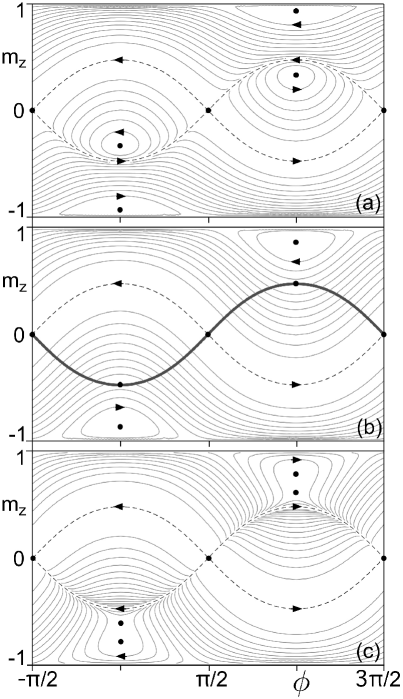
Figure 1: Phase portrait of undamped spin-transfer-driven dynamics under zero external field and increasing spin current. Continuous lines: constant-level curves of integral of motion $\tilde{g}_{{}_{\mathit{\!M}}}$. Arrows: direction of magnetization change. Dashed lines: invariant trajectories $w\pm w_{Q}=0$. Black dots: critical points. (a) $\beta=0.75\,Q$. (b) $\beta=Q$ (bifurcation point), the bold continuous line representing the critical line on which $d\mathbf{m}/dt=0$. (c) $\beta=1.15\,Q$. Parameters: $D_{yx}=0.3$, $D_{zy}=1$, $Q=\sqrt{D_{zy}D_{yx}}$.

To derive this integrating factor, consider that $\tilde{g}_{{}_{\mathit{\!M}}}$, as a conserved quantity, must satisfy the condition: $d\tilde{g}_{{}_{\mathit{\!M}}}/dt=(\partial\tilde{g}_{{}_{\mathit{\!M}}}/\partial\mathbf{m})\cdot(d\mathbf{m}/dt)=0$ along magnetization trajectories, that is (see Eq. (2)):

$$\left(\mathbf{h}_{{}_{\mathit{\!M}}}-\frac{g_{{}_{\mathit{\!M}}}}{f}\,\frac{\partial f}{\partial\mathbf{m}}\right)\cdot\Big{[}\mathbf{m}\times\big{(}\mathbf{h}_{{}_{\mathit{\!M}}}-\beta\,\mathbf{m}\times\mathbf{e}_{y}\big{)}\Big{]}=0\,\,\,.$$ (4)

This condition is identically satisfied for any $\mathbf{m}$ if the vectors $\mathbf{h}_{{}_{\mathit{\!M}}}-\left(g_{{}_{\mathit{\!M}}}/f\right)\partial f/\partial\mathbf{m}$ and $\mathbf{h}_{{}_{\mathit{\!M}}}-\beta\,\mathbf{m}\times\mathbf{e}_{y}$ are parallel, that is, if:

$$\frac{g_{{}_{\mathit{\!M}}}}{f}\,\frac{\partial f}{\partial\mathbf{m}}=\beta\,\mathbf{m}\times\mathbf{e}_{y}\,\,\,.$$ (5)

This equation yields the following differential equation:

$$\frac{1}{f}\,\frac{df}{dw}=\frac{\beta}{Q}\,\,\frac{2w_{Q}}{w^{2}-w_{Q}^{2}}\,\,\,,\,\,\,w=\frac{m_{z}}{m_{x}}\,\,\,,$$ (6)

where: $Q=\sqrt{D_{zy}D_{yx}}$ and $w_{Q}=\sqrt{D_{yx}/D_{zy}}$. Indeed, $\mathbf{m}\times\mathbf{e}_{y}=m_{x}^{2}\,\partial w/\partial\mathbf{m}$ and $g_{{}_{\mathit{\!M}}}(\mathbf{m})=D_{zy}m_{x}^{2}\left(w^{2}-w_{Q}^{2}\right)/2$ (see Eq. (1)). By integrating Eq. (6) under the condition that $f(w;0)\equiv 1$, one obtains:

$$f(w;\beta)=\left|\frac{w-w_{Q}}{w+w_{Q}}\right|^{\beta/Q}\,\,\,.$$ (7)

By using Eq. (5), Eq. (2) is transformed into Eq. (3), as anticipated. The phase portrait of the dynamics is straightforwardly obtained by drawing the constant-level lines of $\tilde{g}_{{}_{\mathit{\!M}}}(\mathbf{m};\beta)\equiv f(w;\beta)\,g_{{}_{\mathit{\!M}}}(\mathbf{m})$ (Fig. 1). A convenient representation is obtained in terms of cylindrical coordinates $(m_{z},\phi)$, whose relation to the cartesian magnetization components $(m_{x},m_{y},m_{z})$ is: $m_{x}=\sqrt{1-m_{z}^{2}}\,\cos\phi$, $m_{y}=\sqrt{1-m_{z}^{2}}\,\sin\phi$.

Figure 1 illustrates the progressive restructuring of the dynamics as the spin current is increased. A remarkable property of this restructuring is the invariance of zero-energy trajectories. According to Eq. (1), constant-level lines on which $g_{{}_{\mathit{\!M}}}=0$ are described by the equations: $m_{z}\sqrt{D_{zy}}\pm m_{x}\sqrt{D_{yx}}=0$. It is easily verified that on these curves $\mathbf{h}_{{}_{\mathit{\!M}}}=\pm Q\,\mathbf{m}\times\mathbf{e}_{y}$. By substituting this expression into Eq. (2) and by taking into account that $\mathbf{h}_{{}_{\mathit{\!M}}}=-\partial g_{{}_{\mathit{\!M}}}/\partial\mathbf{m}$, one obtains:

$$\frac{d\mathbf{m}}{dt}=\left(1\mp\frac{\beta}{Q}\right)\mathbf{m}\times\frac{\partial g_{{}_{\mathit{\!M}}}}{\partial\mathbf{m}}\,\,\,.$$ (8)

This expression reveals that if $g_{{}_{\mathit{\!M}}}=0$, then $dg_{{}_{\mathit{\!M}}}/dt=(\partial g_{{}_{\mathit{\!M}}}/\partial\mathbf{m})\cdot(d\mathbf{m}/dt)=0$. In other words, constant-level curves on which $g_{{}_{\mathit{\!M}}}=0$ are always solutions of the dynamics, whatever the value of the spin current $\beta$. The current only affects the rate at which the constant-level curve is traversed. This rate goes to zero when $\beta=\pm Q$. When this condition is met, the entire constant-level curve becomes a critical line along which $d\mathbf{m}/dt=0$. This occurs as a result of a complex bifurcation (see Fig. 1(b)), at which a global transition from closed to open magnetization trajectories occurs.

The dramatic restructuring of the phase portrait at $\beta=\pm Q$ affects the integral of motion $\tilde{g}_{{}_{\mathit{\!M}}}$, which is single-valued and continuous everywhere for $\beta^{2}<Q^{2}$, while it diverges on the curve $w+w_{Q}=0$ when $\beta>Q$ or on the curve $w-w_{Q}=0$ when $\beta<-Q$. However, this divergence can be eliminated by taking advantage of the fact that any arbitrary monotone function $F(\tilde{g}_{{}_{\mathit{\!M}}})$ can be taken as integral of motion instead of $\tilde{g}_{{}_{\mathit{\!M}}}$. If one chooses $F(\tilde{g}_{{}_{\mathit{\!M}}})=\arctan\tilde{g}_{{}_{\mathit{\!M}}}$, then Eq. (3) is transformed into:

$$\frac{d\mathbf{m}}{d\,t}=\frac{1+\tilde{g}_{{}_{\mathit{\!M}}}^{2}}{f}\,\mathbf{m}\times\frac{\partial}{\partial\mathbf{m}}\arctan\tilde{g}_{{}_{\mathit{\!M}}}\,\,\,.$$ (9)

The function $\arctan\tilde{g}_{{}_{\mathit{\!M}}}$ appears similar to a stream function: it is conserved along magnetization trajectories and exhibits a discontinuous jump of amplitude equal to $\pi$ across the curve on which $\tilde{g}_{{}_{\mathit{\!M}}}$ diverges.

When a magnetic field $h_{a}\mathbf{e}_{y}$ is applied along the intermediate axis $\mathbf{e}_{y}$, the energy of the system becomes $g(\mathbf{m};h_{a})=g_{{}_{\mathit{\!M}}}(\mathbf{m})-h_{a}\,\mathbf{e}_{y}\cdot\mathbf{m}$, and the undamped spin-transfer-driven dynamics is governed, instead of Eq. (3), by the equation:

$$\frac{d\mathbf{m}}{dt}=\frac{1}{f}\,\mathbf{m}\times\frac{\partial\tilde{g}_{{}_{\mathit{\!M}}}}{\partial\mathbf{m}}-h_{a}\,\mathbf{m}\times\mathbf{e}_{y}\,\,\,.$$ (10)

The introduction of the field breaks the $(m_{y},t)$ reversal symmetry and thus destroys the property of $\tilde{g}_{{}_{\mathit{\!M}}}$ of being an integral of motion. However, quite remarkably, it is possible to modify $\tilde{g}_{{}_{\mathit{\!M}}}$ in order to obtain a state function that acts as a global Lyapunov function Andronov et al. (1987); Perko (1996), that is, a function that monotonically increases or decreases under all circumstances during the magnetization process. We shall limit the discussion to the current interval $\beta^{2}<Q^{2}$, in which $\tilde{g}_{{}_{\mathit{\!M}}}$ is a single-valued, well-behaved state function. A different approach, not discussed here, would be necessary to deal with the case when $\beta^{2}>Q^{2}$.

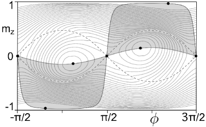
Figure 2: Constant-level curves of function $\tilde{g}(\mathbf{m};\beta,h_{a})$ for $\beta^{2}<Q^{2}$. Dashed lines: curves $w\pm w_{Q}=0$ on which $g_{{}_{\mathit{\!M}}}(\mathbf{m})=0$. Black dots: critical points. Shadowed region: region delimited by curves $w=w_{1}$ and $w=w_{2}$, in which $(f-f_{0})>0$ and $(w-w_{1})(w-w_{2})<0$ (the opposite occurs in remaining non shadowed region). Parameters: $D_{yx}=0.3$, $D_{zy}=1$, $\beta=0.2$, $h_{a}=0.1$, $w_{Q}=\sqrt{D_{zy}/D_{yx}}$.

The time derivative of $\tilde{g}_{{}_{\mathit{\!M}}}$ derived from Eq. (10) is: $d\tilde{g}_{{}_{\mathit{\!M}}}/dt=h_{a}\,f\,dm_{y}/dt$. The term $dm_{y}/dt$ can be computed from Eq. (10). One finds:

$$\frac{1}{1-m_{y}^{2}}\,\frac{dm_{y}}{dt}=-\left(\frac{2Rw}{1+w^{2}}+\beta\right)\,\,\,,$$ (11)

where $w=m_{z}/m_{x}$ and $R=\left(D_{zy}+D_{yx}\right)/2$. Equation (11) shows that the sign of $dm_{y}/dt$ is fully controlled by the roots of the equation $w^{2}+2Rw/\beta+1=0$, namely, $w_{1,2}=-\left(R\mp\sqrt{R^{2}-\beta^{2}}\right)/\beta$. When $\beta^{2}<Q^{2}<R^{2}$, $w_{1}^{2}<w_{Q}^{2}$ and $w_{2}^{2}>w_{Q}^{2}$. Therefore, the curve $w=w_{1}$ lies in the region $g_{{}_{\mathit{\!M}}}<0$ and the curve $w=w_{2}$ in the region $g_{{}_{\mathit{\!M}}}>0$, since $g_{{}_{\mathit{\!M}}}(\mathbf{m})=D_{zy}m_{x}^{2}\left(w^{2}-w_{Q}^{2}\right)/2$ (see Eq. (1) and Fig. 2).

Consider now the function:

$$\tilde{g}\left(\mathbf{m};\beta,h_{a}\right)=$$ (12)

$$\tilde{g}_{{}_{\mathit{\!M}}}(\mathbf{m};\beta)-f_{0}h_{a}\mathbf{e}_{y}\cdot\mathbf{m}\,\,\,,\,\,\,f_{0}=\left\{\begin{array}[]{c}f(w_{1};\beta)\,\,\,\text{if}\,\,\,g_{{}_{\mathit{\!M}}}\leq 0\\ f(w_{2};\beta)\,\,\,\text{if}\,\,\,g_{{}_{\mathit{\!M}}}>0\end{array}\right..$$ (15)

Its time derivative, computed from Eq. (10), is: $d\tilde{g}/dt=h_{a}\left(f-f_{0}\right)dm_{y}/dt$, at every point in state space at which $g_{{}_{\mathit{\!M}}}\neq 0$. By combining this result with Eq. (11), one arrives at:

$$\frac{d\tilde{g}}{dt}=-\beta h_{a}\,\frac{1-m_{y}^{2}}{1+w^{2}}\,\big{(}f-f_{0}\big{)}\big{(}w-w_{1}\big{)}\big{(}w-w_{2}\big{)}\,\,\,.$$ (16)

By definition of $f(w;\beta)$ (Eq. (7)) and $f_{0}$ (Eq. (12)), $(f-f_{0})>0$ when $(w-w_{1})(w-w_{2})<0$ and vice versa (see Fig. 2). Therefore, the function $\tilde{g}(\mathbf{m};\beta,h_{a})$ will be an increasing or decreasing function of time, depending on whether the product $\beta h_{a}$ is positive or negative, respectively. In particular, the maxima and minima of $\tilde{g}$ will represent critical points of the dynamics (Fig. 2). When $\beta=0$ or $h_{a}=0$, $\tilde{g}$ is reduced to the corresponding conserved quantity, $g(\mathbf{m};h_{a})$ or $\tilde{g}_{{}_{\mathit{\!M}}}(\mathbf{m};\beta)$, respectively.

Equation (16) is not valid when $g_{{}_{\mathit{\!M}}}=0$, because $\tilde{g}$ is discontinuous there as a consequence of the jump in $f_{0}$. However, this discontinuity does not modify the conclusions of our analysis. It is sufficient to complement Eq. (16) with the information about the direction of crossing of the boundary $g_{{}_{\mathit{\!M}}}=0$. This information is readily obtained from the dynamics of the ratio $w=m_{z}/m_{x}$. From Eq. (10) one finds that if $w\pm w_{Q}=0$, then $dw/dt=-\left(1+w_{Q}^{2}\right)h_{a}$. Thus, the boundary $g_{{}_{\mathit{\!M}}}=0$ is crossed in the sense of decreasing $w$ when $h_{a}>0$ and increasing $w$ when $h_{a}<0$.

The existence of the function $\tilde{g}$ implies that the undamped spin-transfer-driven dynamics under nonzero field is nothing but a field-induced relaxation process toward $\tilde{g}$ minima or maxima, depending on the sign of the product $\beta h_{a}$. The function $\tilde{g}$ is characterised by a pair of minima in the region $g_{{}_{\mathit{\!M}}}<0$ and a pair of maxima in the region $g_{{}_{\mathit{\!M}}}>0$ Not . Therefore, there will exist two basins of attraction for the field-induced relaxation. These basins exhibit some degree of interlacing, similarly to what one observes in conventional magnetization relaxation due to intrinsic damping Bertotti et al. (2013), the smaller the field $h_{a}$, the finer the interlacing. An example, obtained by numerical integration of Eq. (10), is shown in Fig. 3. The fine basin interlacing makes the field-induced relaxation probabilistic in nature whenever control of initial conditions is imperfect Neishtadt (1991); Arnold et al. (2006). We stress that intrinsic damping has been neglected in the derivation of these results.

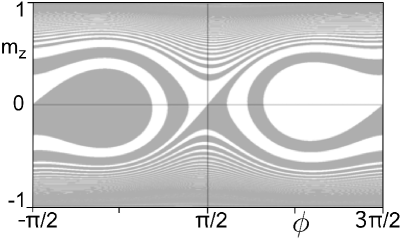
Figure 3: Basins of attraction of undamped spin-transfer-driven dynamics under nonzero external magnetic field. Parameters: $D_{yx}=0.3$, $D_{zy}=1$, $\beta=0.05$, $h_{a}=-0.025$.

Intrinsic damping effects can be conveniently introduced in so-called Gilbert form Gilbert (2004); Tserkovnyak et al. (2005); Hickey and Moodera (2009), which amounts to changing $d\mathbf{m}/dt$ into $d\mathbf{m}/dt-\alpha\,\mathbf{m}\times d\mathbf{m}/dt$ in Eq. (10). As a consequence, Eq. (16) is modified as:

$$\frac{d\tilde{g}}{dt}=-\alpha\,f\left|\frac{d\mathbf{m}}{dt}\right|^{2}+h_{a}\left(f-f_{0}\right)\frac{dm_{y}}{dt}\,\,\,,$$ (17)

where $\alpha$ represents the damping constant. The last term on the right-hand side of Eq. (17) is not exactly coincident with the right-hand side of Eq. (16), because $dm_{y}/dt$ is slightly modified by the introduction of damping. However, this modification plays a secondary role if $\alpha\ll 1$. In essence, Eq. (17) is controlled by two terms, of which the one due to damping is always negative whereas the one due to current and field is approximately equal to the right-hand side of Eq. (16) and has thus the sign of the product $\beta h_{a}$. Hence, when current and field have opposite sign, their action contributes jointly with intrinsic damping to the stabilization of $\tilde{g}$ minima, whereas when they have identical sign their action competes with that of intrinsic damping.

There exist conditions under which damping-induced and field-induced relaxations balance each other, leading to the appearance of limit cycles, that is, of magnetization self-oscillations. A typical scenario, confirmed by computer simulations, is the formation of a pair of attractive/repulsive limit cycles through a semi-stable limit-cycle bifurcation Kuznetsov (1995); Perko (1996). Depending on the values of field and current, hysteretic transitions may occur between coexisting stationary and self-oscillation regimes, or conditions can be realised in which all critical points are unstable, which means that self-oscillations become the only possible steady-state regime available to the system.

This work was partially supported by Progetto Premiale MIUR-INRIM Nanotecnologie per la metrologia elettromagnetica , by MIUR-PRIN Project 2010ECA8P3 DyNanoMag , and by NSF.

References

- Slonczewski (1996) J. C. Slonczewski, J. Magn. Magn. Mater. 159, L1 (1996).
- Berger (1996) L. Berger, Phys. Rev. B 54, 9353 (1996).
- Tserkovnyak et al. (2005) Y. Tserkovnyak, A. Brataas, G. E. W. Bauer, and B. I. Halperin, Rev. Mod. Phys. 77, 1375 (2005).
- Haney et al. (2008) P. M. Haney, R. A. Duine, A. S. Nunez, and A. H. MacDonald, J. Magn. Magn. Mater. 320, 1300 (2008).
- Brataas et al. (2012) A. Brataas, A. D. Kent, and H. Ohno, Nature Mater. 11, 372 (2012).
- Katine et al. (2000) J. A. Katine, F. J. Albert, R. A. Buhrman, E. B. Myers, and D. C. Ralph, Phys. Rev. Lett. 84, 3149 (2000).
- Bazaliy et al. (2004) Y. B. Bazaliy, B. A. Jones, and S. C. Zhang, Phys. Rev. B 69, 094421 (2004).
- Kubota et al. (2008) H. Kubota, A. Fukushima, K. Yakushiji, T. Nagahama, S. Yuasa, K. Ando, H. Maehara, Y. Nagamine, K. Tsunekawa, D. D. Djayaprawira, et al., Nature Physics 4, 37 (2008).
- Liu et al. (2012) L. Liu, C. F. Pai, Y. Li, H. W. Tseng, D. C. Ralph, and R. A. Buhrman, Science 336, 555 (2012).
- Kiselev et al. (2003) S. I. Kiselev, J. C. Sankey, I. N. Krivorotov, N. C. Emley, R. J. Schoelkopf, R. A. Buhrman, and D. C. Ralph, Nature 425, 380 (2003).
- Rippard et al. (2004) W. H. Rippard, M. R. Pufall, S. Kaka, S. E. Russek, and T. J. Silva, Phys. Rev. Lett. 92, 027201 (2004).
- Krivorotov et al. (2005) I. N. Krivorotov, N. C. Emley, J. C. Sankey, S. I. Kiselev, D. C. Ralph, and R. A. Buhrman, Science 307, 228 (2005).
- Bertotti et al. (2005) G. Bertotti, C. Serpico, I. D. Mayergoyz, A. Magni, M. d’Aquino, and R. Bonin, Phys. Rev. Lett. 94, 127206 (2005).
- Bertotti et al. (2009) G. Bertotti, I. D. Mayergoyz, and C. Serpico, Nonlinear Magnetization Dynamics in Nanosystems (Elsevier, Oxford, 2009).
- Li et al. (2005) Z. Li, J. He, and S. Zhang, Phys. Rev. B 72, 212411 (2005).
- Andronov et al. (1987) A. A. Andronov, A. A. Vitt, and S. E. Khaikin, Theory of Oscillators (Dover, New York, 1987).
- Perko (1996) L. Perko, Differential Equations and Dynamical Systems (Springer, New York, 1996).
- (18) A detailed analysis, not reported here, shows that this occurs in the current-field region: , where and .
- Bertotti et al. (2013) G. Bertotti, C. Serpico, and I. D. Mayergoyz, Phys. Rev. Lett. 110, 147205 (2013).
- Neishtadt (1991) A. I. Neishtadt, Chaos 1, 42 (1991).
- Arnold et al. (2006) V. I. Arnold, V. V. Kozlov, and A. I. Neishtadt, Mathematical Aspects of Classical and Celestial Mechanics (Springer, Berlin, 2006).
- Gilbert (2004) T. L. Gilbert, IEEE Trans. Magn. 40, 3443 (2004).
- Hickey and Moodera (2009) M. C. Hickey and J. S. Moodera, Phys. Rev. Lett. 102, 137601 (2009).
- Kuznetsov (1995) Y. A. Kuznetsov, Elements of Applied Bifurcation Theory (Springer, New York, 1995).