Phase-field-crystal models and mechanical equilibrium

Abstract

Phase field crystal (PFC) models constitute a field theoretical approach to solidification, melting and related phenomena at atomic length and diffusive time scales. One of the advantages of these models is that they naturally contain elastic excitations associated with strain in crystalline bodies. However, instabilities that are diffusively driven towards equilibrium are often orders of magnitude slower than the dynamics of the elastic excitations, and are thus not included in the standard PFC model dynamics. We derive a method to isolate the time evolution of the elastic excitations from the diffusive dynamics in the PFC approach and set up a two-stage process, in which elastic excitations are equilibrated separately. This ensures mechanical equilibrium at all times. We show concrete examples demonstrating the necessity of the separation of the elastic and diffusive time scales. In the small deformation limit this approach is shown to agree with the theory of linear elasticity.

I Introduction

Insight into crystal growth and related phenomena is essential for understanding fundamental material properties and exploiting them in engineering applications. Atomistic methods such as density functional theory (both quantum-mechanical and classical), or numerical molecular dynamics simulations have provided a great deal of information about material properties but are limited to relatively small length and time scales. Thermally driven dynamics such as annealing of defects or relaxing stress in heteroepitaxial systems requires microsecond time scales that are beyond such methods. On large length scales there are a vast number of macroscopic field theories for studying melting and solidification but these theories often fail to incorporate atomistic details that are essential for understanding the phenomena associated with crystal growth. To this end the phase field crystal (PFC) model was proposed by Elder et al. Elder et al. (2002); Elder and Grant (2004); Elder et al. (2007) to add a richer theory able to describe the underlying crystalline structure with elastic and plastic properties. The PFC model describes the dynamics of a dimensionless field $n$ that is related to the atomic number density and as such is periodic in a crystalline state and constant in a liquid phase. PFC models have been applied to study a wide range of different phenomena such as grain-boundary melting Berry et al. (2008a); Mellenthin et al. (2008) and energy Jaatinen et al. (2009), fractal growth Tegze et al. (2011), surface ordering Achim et al. (2006, 2009); Ramos et al. (2010, 2008), epitaxial growth Elder et al. (2002); Elder and Grant (2004); Elder et al. (2007); Wu and Voorhees (2009), the yield stress of polycrystals Stefanovic et al. (2006); Hirouchi et al. (2009); Stefanovic et al. (2009) and glass transitions Berry et al. (2008b); Berry and Grant (2011).

The dynamics of the PFC model were originally assumed to be conserved dissipative and driven by the chemical potential to minimize an associated free energy functional. Such dynamics can in certain limits be justified by more fundamental arguments Marconi and Tarazona (1999); Archer and Evans (2004); Majaniemi and Grant (2007). However, since the energy of the PFC models incorporates elastic energy due to elastic stress this might turn out to be problematic in some cases. For example, elastic excitations such as travelling wave modes and simple stretch or compression of solid body should relax considerably faster than the diffusive time scales of solidification. Even in a system that is actively not driven out of equilibrium elastic excitations can arise. For example, crystallization from multiple crystallization centres may result into elastic excitations when the grains that are oriented in different directions meet at the grain boundaries. It is often justifiably assumed that in many materials (metals, insulators, semi-conductors) elastic equilibrium is instantaneous compared to the other slow processes, such as solidification, phase segregation, etc. Attempts have been made to address this issue by adding higher time derivatives to the PFC equation Stefanovic et al. (2006), but such an approach is only approximate. In this work we present a method that can be shown to give exact elastic or mechanical equilibrium in the small deformation limit. This approach relies on the so-called amplitude formulation of the PFC model.

The amplitude formulation bridges the gap between the conventional PFC model and more macroscopic phase field models and was introduced by Goldenfeld and collaborators Goldenfeld et al. (2005); Athreya et al. (2006); Goldenfeld et al. (2006) for the two dimensional triangular phase of the PFC model and has been extended to three dimensional bcc and fcc crystals, binary alloys Elder et al. (2010); Huang et al. (2010) and to include miscibility gap in the density field Yeon et al. (2010). This approach considers variations of the amplitudes of a periodic density field. The amplitudes are complex so that they have two degrees of freedom, magnitude and phase. Essentially, the magnitude of the amplitude is zero in the liquid state and finite in a crystalline phase, while the phase can account for elastic deformations and rotations. The combination of the two can describe dislocations and grain boundaries, since the phase can be discontinuous when the magnitude goes to zero. This approach allows for larger length and time scales, and as shown by Athera et al. Athreya et al. (2007) can be numerically implemented using efficient multi-grid methods. It is also very useful for studies in which the crystal orientation is almost the same everywhere (except near dislocations) as in the case of heteroepitaxial systems Huang and Elder (2008, 2010); Elder et al. (2012, 2013).

In this article we propose a method to isolate and separately equilibrate the elastic excitations of the system within the framework of the amplitude expansion of the PFC model and show that in a certain limit this is consistent with elastic equilibrium. Numerical verification of the theory is also provided. The article is organized as follows: Sec. II introduces the phase-field crystal model and its corresponding amplitude expansion. The separation of the fast time scales associated with elastic excitations is described in Sec. III and later studied in the linear deformation limit in Sec. IV. The theory is numerically tested in Sec. V and finally the results are summarized and concluded in Sec. VI.

II Phase-field crystal model

The phase-field crystal model Elder et al. (2002); Elder and Grant (2004); Elder et al. (2007) is a coarse-grained model that describes the dynamics of a dimensionless field $n$ that is related to deviations of the atomic number density from the average number density. The associated free energy can be written in dimensionless form as

$$\begin{split}F_{PFC}[n(\vec{r})]&=\int_{\Omega}d\vec{r}\left\{\frac{\Delta B}{2}n(\vec{r})^{2}+B^{x}\frac{n}{2}(1+\nabla^{2})^{2}n\right.\\ &\left.-\frac{\tau}{3}n^{3}+\frac{v}{4}n^{4}\vphantom{\frac{\Delta B}{2}}\right\},\end{split}$$ (1)

where $\Delta B\equiv B^{\ell}-B^{x}$. The parameter $B^{\ell}$ is related to the compressibility of the liquid state, and the elastic moduli of the crystalline state are proportional to $B^{x}$. The parameters $\tau$ and $v$ control the amplitude of the fluctuations in the solid state and the liquid-solid miscibility gap. Descriptions of these parameters can be found in Refs. Jaatinen et al. (2009); Elder et al. (2007). The field $n$ is a conserved quantity that is driven to minimize the free energy, i.e.,

$$\begin{split}\frac{dn}{dt}&=\nabla^{2}\frac{\delta F_{PFC}}{\delta n}\\ &=\nabla^{2}\left[\Delta Bn+B^{x}(1+\nabla^{2})^{2}n-\tau n^{2}+vn^{3}\right],\end{split}$$ (2)

where the mobility has been set to unity. As discussed in many previous works, the free energy functional has an elastic contribution and Eq. (2) does relax to minimize any elastic deformations. However, the relaxation is on diffusive times scales, not on time scales associated with phonon modes (or speed of sound time scales) that can be significantly faster in metals and semiconductors. It is often assumed that the relaxation is instantaneous compared to processes such as vacancy diffusion or solidification in traditional phase field models of such systems Muller and Grant (1999); Haataja et al. (2002); Orlikowski et al. (1999); Wang et al. (2001).

To see how instantaneous elastic equilibrium can be achieved it is useful to consider an amplitude representation of $n$ and the corresponding equations of motion. In the solid phase the ground state can be represented in an amplitude expansion, i.e.,

$$n\approx\bar{n}+\sum_{j}\left[\eta_{j}(\vec{r},t)e^{i\vec{q}_{j}\cdot\vec{r}}+\textrm{c.c.}\right],$$ (3)

where $\eta_{j}$ are complex amplitudes, $\vec{q}_{j}\equiv{\rm k}\,\vec{k}_{1}+{\rm l}\,\vec{k}_{2}+{\rm m}\,\vec{k}_{3}$, (klm) are the Miller indices and $(\vec{k}_{1},\vec{k}_{2},\vec{k}_{3}$) are the principle reciprocal lattice vectors. Within a certain range of parameters, Eq. (1) produces a triangular crystal lattice in two dimensions as a ground state that to a good approximation can be approximated by only three amplitudes, the ones corresponding to the three smallest $|\vec{q}_{j}|$’s. More generally, equations of motion for the amplitudes have been derived using various methods by assuming that they are slowly varying functions of space and times. This procedure is described in detail in Refs. Athreya et al. (2006); Goldenfeld et al. (2006, 2005); Yeon et al. (2010); Elder et al. (2010); Huang et al. (2010).

The reason it is interesting to consider the complex amplitudes as opposed to $n$ itself is that the magnitude and phase of $\eta_{j}$ describe different physical features and more importantly naturally separate out the elastic part, as will be explained in the next section. This separation makes it possible to relax the elastic energy at a different rate than other processes, such as vacancy diffusion and climb. The separation of time scales is discussed in the next section.

III Amplitude expansion

A simple derivation of the equations of motion of the amplitudes can be obtained by assuming that the amplitudes are approximately constant at atomic length scales. This is done by substituting Eq. (3) into Eq. (2), multiplying by $e^{-i\vec{q}_{j}\cdot\vec{r}}$ and averaging over one unit cell, assuming that the $\eta_{j}$’s are constant. This heuristic method gives essentially the same result as more rigorous multiple scales or renormalization group calculations. The results of such calculations give the dynamic amplitude equations for a single component 2D system Elder et al. (2010),

$$\begin{split}\frac{d\eta_{j}}{dt}&=-\left\{\vphantom{\prod_{i\neq j}}\left[\Delta B+B^{x}\mathcal{G}_{j}^{2}+3v(A^{2}-|\eta_{j}|^{2})\right]\eta_{j}\right.\\ &\left.-2\tau\prod_{i\neq j}\eta_{i}^{*}\right\},\end{split}$$ (4)

where

$$\mathcal{G}_{j} \equiv \nabla^{2}+2i\vec{q}_{j}\cdot\vec{\nabla},$$ (5)

$$A^{2} \equiv 2\sum_{j}|\eta_{j}|^{2},$$ (6)

$$\vec{q}_{1} = -\sqrt{3}\hat{x}/2-\hat{y}/2,$$ (7)

$$\vec{q}_{2} = \hat{y},$$ (8)

$$\vec{q}_{3} = \sqrt{3}\hat{x}/2-\hat{y}/2.$$ (9)

The time evolution can also be written by using the (dimensionless) free energy as

$$\frac{d\eta_{j}}{dt}=-\frac{\delta F}{\delta\eta_{j}^{*}},$$ (10)

with the free energy

$$\begin{split}F[\{\eta_{j}\}]&=\int_{\Omega}d\vec{r}\left\{\frac{\Delta B}{2}A^{2}+\frac{3v}{4}A^{4}\right.\\ &\left.+\sum_{j=1}^{3}\left[B^{x}|\mathcal{G}_{j}\eta_{j}|^{2}-\frac{3v}{2}|\eta_{j}|^{4}\right]\right.\\ &\left.-2\tau(\eta_{1}\eta_{2}\eta_{3}+\eta_{1}^{*}\eta_{2}^{*}\eta_{3}^{*})\vphantom{\frac{\Delta B}{2}}\right\}.\end{split}$$ (11)

It should be noted that $|\vec{q}_{j}|=1$, which is a direct consequence of the term $(1+\nabla^{2})^{2}$ in the PFC energy defined by Eq. (1). This sets the length scale throughout the article.

The complex amplitudes represent renormalized amplitudes of a one-mode approximation of the number density field associated with the PFC models. The approximate PFC density field can be reconstructed from Eq. (3). A perfect crystal can be realized by setting $\eta_{j}=\phi=\textit{constant}$. This helps in the interpretation of the complex amplitudes. Consider a deformation of the coordinates $\vec{r}\to\vec{r}+\vec{u}$ with some deformation field $\vec{u}(\vec{r})$. Making this substitution in $n$ is equivalent to transforming the amplitudes of the perfect crystal to $\eta_{j}=\phi\exp{(i\vec{q}_{j}\cdot\vec{u})}$. Thus we see that the phase of the amplitude carries information about the deformation field $\vec{u}$. For this reason it is useful to write $\eta_{j}=\phi_{j}\exp(i\theta_{j})$ and consider the equations of motion for $\phi_{j}$ and $\theta_{j}$ separately.

Writing $\eta_{j}=\phi_{j}\exp{(i\theta_{j})}$ the complex amplitudes can be separated into fields $\phi_{j}(\vec{r},t)$ that differentiate between the liquid and solid phase, and fields $\theta_{j}(\vec{r},t)$ that represent deformations. The idea behind the separation of the time scales is that the fields $\phi_{j}(\vec{r},t)$ represent slow melting, solidification and diffusive phenomena while the fields $\theta_{j}(\vec{r},t)$ stand for deformations that are in general fast. It is then straightforward to show that Eq. (4) becomes

$$\begin{split}\frac{d\phi_{j}}{dt}+i\phi_{j}\frac{d\theta_{j}}{dt}&=-B^{x}(\mathcal{L}_{j}^{2}-4\mathcal{Q}_{j}^{2}+4i\mathcal{Q}_{j}\mathcal{L}_{j})\phi_{j}\\ &-\Delta B\phi_{j}-3v\left(2\sum_{i}(\phi_{i}^{2})-\phi_{j}^{2}\right)\phi_{j}\\ &+2\tau\left(\prod_{i\neq j}\phi_{i}\right)\exp{\left(-i\sum_{i}\theta_{i}\right)},\end{split}$$ (12)

where $\mathcal{Q}_{j}$ and $\mathcal{L}_{j}$ are operators given by

$$\mathcal{Q}_{j}\equiv\vec{q}_{j}\cdot\left(\vec{\nabla}+i\vec{\nabla}\theta_{j}\right),$$ (13)

and

$$\mathcal{L}_{j}\equiv\nabla^{2}-|\vec{\nabla}\theta_{j}|^{2}+2i\vec{\nabla}\theta_{j}\cdot\vec{\nabla}+i\nabla^{2}\theta_{j}.$$ (14)

Collecting the real and the imaginary parts of the right-hand side of Eq. (12) gives the equations of motion for $\phi_{j}$ and $\theta_{j}$. To understand the behavior of the fields and their relationship to elastic equilibrium it is useful to consider next the limit of a small deformation.

IV Small deformation limit

In the small deformation limit the complex amplitudes can be represented as $\eta_{j}=\phi e^{i\vec{q}_{j}\cdot\vec{u}}$, where $\vec{u}$ is the standard displacement vector used in continuum elasticity theory Landau et al. (1986). If we consider the case in which the derivatives of $\vec{u}$ are of linear order and $\phi$ is constant in time and space, it is then straightforward to determine the conditions in which elastic equilibrium is reached. In the next section these conditions are derived by varying the free energy with respect to the strain tensor to determine the stress tensor and then imposing the standard definition of elastic equilibrium, i.e., that the divergence of the stress tensor is zero. In subsection IV.2 it is also shown that this is equivalent to a condition on the dynamics of the phases $\theta_{j}$. In this way new equations for the dynamics of the phases can be introduced to ensure exact elastic equilibrium in the small deformation limit.

IV.1 Elastic equilibrium from energy

In the linear elastic limit the elastic equilibrium is written in terms of the linear strain tensor

$$\varepsilon_{ij}=\frac{1}{2}\left(\frac{\partial u_{i}}{\partial x_{j}}+\frac{\partial u_{j}}{\partial x_{i}}\right),$$ (15)

where $u_{i}$ are the components of the deformation field $\vec{u}$ and the stress tensor that can be obtained by taking a tensor derivative of the free energy with respect to the strains, i.e.,

$$\sigma_{ij}=\begin{cases}\frac{\delta F}{\delta\varepsilon_{ij}}&\text{if $i=j$};\\ \frac{1}{2}\frac{\delta F}{\delta\varepsilon_{ij}}&\text{if $i\neq j$}.\end{cases}$$ (16)

Elastic equilibrium is then established when,

$$\vec{\nabla}\cdot\vec{\vec{\sigma}}=0.$$ (17)

The above equation is Newton’s second law of motion for continuum media in the static case.

As shown in a prior publication Elder et al. (2010), for a two dimensional triangular lattice the elastic contribution to the free energy given in Eq. (11) can be written as

$$\begin{split}F_{el}&=\int d\vec{r}\left[3B^{x}\phi^{2}\left(\frac{3}{2}\varepsilon_{11}^{2}+\frac{3}{2}\varepsilon_{22}^{2}+\varepsilon_{11}\varepsilon_{22}+2\varepsilon_{12}^{2}\right)\right].\end{split}$$ (18)

Using this we can write down the components of the stress tensor from Eq. (16)

$$\begin{split}\sigma_{11}=3B^{x}\phi^{2}(3\varepsilon_{11}+\varepsilon_{22})=3B^{x}\phi^{2}(3\partial_{1}u_{1}+\partial_{2}u_{2}),\end{split}$$ (19)

$$\begin{split}\sigma_{22}=3B^{x}\phi^{2}(3\varepsilon_{22}+\varepsilon_{11})=3B^{x}\phi^{2}(\partial_{1}u_{1}+3\partial_{2}u_{2}),\end{split}$$ (20)

and

$$\begin{split}\sigma_{12}=6B^{x}\phi^{2}\varepsilon_{12}=3B^{x}\phi^{2}(\partial_{1}u_{2}+\partial_{2}u_{1}).\end{split}$$ (21)

Elastic equilibrium follows from using Eq. (17) as

$$(\vec{\nabla}\cdot\vec{\vec{\sigma}})_{1}=3B^{x}\phi^{2}(3\partial_{1}^{2}u_{1}+\partial_{2}^{2}u_{1}+2\partial_{1}\partial_{2}u_{2})=0,$$ (22)

$$(\vec{\nabla}\cdot\vec{\vec{\sigma}})_{2}=3B^{x}\phi^{2}(3\partial_{2}^{2}u_{2}+\partial_{1}^{2}u_{2}+2\partial_{1}\partial_{2}u_{1})=0,$$ (23)

simplifying to

$$3\partial_{1}^{2}u_{1}+\partial_{2}^{2}u_{1}+2\partial_{1}\partial_{2}u_{2} =0,$$ (24)

$$3\partial_{2}^{2}u_{2}+\partial_{1}^{2}u_{2}+2\partial_{1}\partial_{2}u_{1} =0.$$ (25)

These equations describe the elastic equilibrium conditions for triangular crystal systems, where the linear strain tensor is connected to the stress via elastic constants as

$$\sigma_{ii}=C_{11}\varepsilon_{ii}+C_{12}\varepsilon_{jj},\quad\textrm{for $i\neq j$};$$ (26)

$$\sigma_{12}=\sigma_{21}=2C_{44}\varepsilon_{12}.$$ (27)

The above calculations give the elastic constants the values of $C_{11}=9B^{x}\phi^{2}$, $C_{12}=3B^{x}\phi^{2}$, and $C_{44}=3B^{x}\phi^{2}$.

IV.2 Elastic equilibrium from dynamical equations

Eq. (12) gives the time evolution for the fields $\phi_{j}$ and $\theta_{j}$. In the limit that $\phi$ is constant in space and time the real and imaginary parts of Eq.  (12) become,

$$4\vec{q}_{j}\cdot\vec{\nabla}\nabla^{2}\theta_{j}=C,$$ (28)

and

$$\frac{d\theta_{j}}{dt}=-B^{x}\left(\nabla^{4}-4(\vec{q}_{j}\cdot\vec{\nabla})^{2}\right)\theta_{j},$$ (29)

respectively, where $C\equiv\Delta B\phi-2\tau\phi^{2}+15v\phi^{3}$. In the small deformation limit, $\theta_{j}\equiv\vec{q}_{j}\cdot\vec{u}$, Eq. (28) for $j=2$ becomes

$$4B^{x}\partial_{2}\nabla^{2}u_{2}=C,$$ (30)

which implies

$$\partial_{2}^{2}\nabla^{2}u_{2}=\partial_{1}\partial_{2}\nabla^{2}u_{2}=0.$$ (31)

Similarly, by adding Eq. (28) for $j=1$ and $j=3$ it is easy to show that

$$\partial_{1}^{2}\nabla^{2}u_{1}=\partial_{2}\partial_{1}\nabla^{2}u_{1}=0.$$ (32)

In addition, subtracting Eq. (28) for $j=1$ and $j=3$ gives

$$\partial_{1}\nabla^{2}u_{2}=-\partial_{2}\nabla^{2}u_{1}.$$ (33)

By taking derivatives of this equation and using Eqns. (31) and (32) it is straightforward to show that

$$\partial^{2}_{1}\nabla^{2}u_{2}=\partial^{2}_{2}\nabla^{2}u_{1}=0$$ (34)

or $\nabla^{4}\vec{u}=0$ which implies $\nabla^{4}\theta_{j}=0$. Thus Eq. (29) to becomes simply

$$\frac{d\theta_{j}}{dt}=4B^{x}(\vec{q}_{j}\cdot\vec{\nabla})^{2}\theta_{j}.$$ (35)

In the small deformation limit the deformation field $\vec{u}$ can be written as

$$\vec{u}=\frac{2}{3}\sum_{j=1}^{3}\vec{q}_{j}\theta_{j}$$ (36)

using deformations along reciprocal lattice vectors $\vec{q}_{j}$ given by $\theta_{j}=\vec{q}_{j}\cdot\vec{u}$. The condition for elastic equilibrium becomes

$$\frac{d\vec{u}}{dt}=\frac{2}{3}\sum_{j=1}^{3}\vec{q}_{j}\frac{d\theta_{j}}{dt}=0.$$ (37)

For a two-dimensional triangular system we have

$$\begin{split}\sum_{j=1}^{3}q_{j1}\frac{d\theta_{j}}{dt}&=\frac{\sqrt{3}}{2}\frac{d\theta_{3}}{dt}-\frac{\sqrt{3}}{2}\frac{d\theta_{1}}{dt}\\ &=\frac{3B^{x}}{2}\left(3\partial_{1}^{2}u_{1}+\partial_{2}^{2}u_{1}+2\partial_{1}\partial_{2}u_{2}\right)\\ &=\frac{1}{2\phi^{2}}(\vec{\nabla}\cdot\vec{\vec{\sigma}})_{1},\end{split}$$ (38)

and

$$\begin{split}\sum_{j=1}^{3}q_{j2}\frac{d\theta_{j}}{dt}&=\frac{d\theta_{2}}{dt}-\frac{1}{2}\frac{d\theta_{1}}{dt}-\frac{1}{2}\frac{d\theta_{3}}{dt}\\ &=\frac{3B^{x}}{2}(3\partial_{2}^{2}u_{2}+\partial_{1}^{2}u_{2}+2\partial_{1}\partial_{2}u_{1})\\ &=\frac{1}{2\phi^{2}}(\vec{\nabla}\cdot\vec{\vec{\sigma}})_{2}.\end{split}$$ (39)

Thus setting

$$\sum\vec{q}_{j}\frac{d\theta_{j}}{dt}=0$$ (40)

ensures elastic equilibrium as defined by Eqs. (22) and (23) or Eqs. (24) and (25). In Appendices A, B, and C we derive the corresponding equations for the one-dimensional case, and for bcc and fcc crystals in three dimensions.

The goal here is to develop a method that incorporates elasticity, dislocations, crystallization and all the features contained in the PFC and related amplitude models that is also consistent with instantaneous elastic equilibrium. This can be achieved by solving Eq. (12) subject to condition given by Eq. (40). To test our approach we have performed numerical calculations for some selected systems, where we expect the mechanical equilibrium constraint to influence the dynamics. A description of these calculations are given in the next section.

V Numerical tests

In this section we discuss the time evolution of the amplitudes using standard conjugate gradient dynamics as described by Eq. (4), and dynamics subject to the elastic equilibrium condition Eq.  (40). The corresponding 1D equations are (100) and (103) in Appendix C.

Eq. (4) and its one dimensional counterpart (100) were solved using a semi-implicit time stepping scheme, where the nonlinear terms of the dynamical equations are treated explicitly while the linear terms are treated implicitly. The spatial derivatives were calculated using fast Fourier transforms. Evolution of the amplitudes according to Eq. (4) is referred to as standard conjugate gradient dynamics while the other approach used is time evolution with elastic equilibration. Numerically the elastic equilibration is formulated as follows.

V.1 Elastic equilibration

For a two dimensional triangular system it is straightforward to show that Eq. (40) can be written as

$$-\frac{d\theta_{i}}{dt}+\frac{1}{2}\left(\frac{d\theta_{j}}{dt}+\frac{d\theta_{k}}{dt}\right)=0,$$ (41)

with $i$, $j$ and $k$ being different. Applying the chain rule shows that these time derivatives can be written down as functional derivatives of the energy defined by Eq. (11) as

$$\frac{d\theta_{j}}{dt}=-\operatorname{Im}{\left[\frac{1}{\eta_{j}}\frac{\delta F}{\delta\eta^{*}}\right]}=-\frac{1}{2}\frac{\delta F}{\delta\theta_{j}}\phi_{j}^{-2}.$$ (42)

Thus the elastic equilibrium condition Eq. (40) can be written as

$$-\frac{\delta F}{\delta\theta_{i}}\phi_{i}^{-2}+\frac{1}{2}\left(\frac{\delta F}{\delta\theta_{j}}\phi_{j}^{-2}+\frac{\delta F}{\delta\theta_{k}}\phi_{k}^{-2}\right)=0.$$ (43)

The algorithm works as follows:

1. Set the initial configuration.

2. Equilibrate $\theta_{i}$ for all $i$ by solving Eq. (43).

3. Calculate time evolution using Eq. (4) for one step.

4. Go to 2.

In 1D the elastic equilibration is simpler. We directly minimize the energy with respect to $\theta$ i.e. the deformation field as

$$\frac{\delta F_{1D}}{\delta\theta}=0,$$ (44)

The energy $F_{1D}$ is defined by Eq. (99).

For numerical calculations the functional derivatives with respect to $\theta$ in both the 1D and the 2D cases are calculated by taking the imaginary part of the conjugate gradient time evolution as suggested by Eq. (42).

V.2 Compression in one dimension

Here we describe a test of the dynamics with elastic equilibrium imposed as described in App. C. We start with a compressed solid body immersed in an undercooled liquid as seen in Figs. 1 and 2 . For the numerical work in this paper we used the dimensionless parameters $\Delta B=-0.5$, $B^{x}=1$ and $v=1$. The size of the 1D system here is $256$ and the spatial discretisation size is about $1.57$. We used a time step of $0.05$ for the evolution of the complex amplitudes.

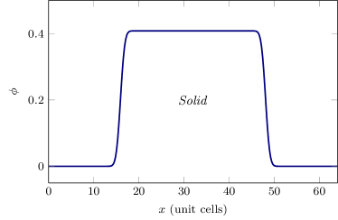
Figure 1: Initial order parameter field: a solid block immersed in an undercool.

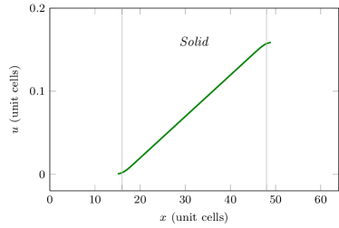
Figure 2: Initial deformation field of the compressed 1D system.

The ground state of the system is a solid block with constant $\phi\approx 0.408$. The evolution of $\phi$ is straightforward as it freezes towards the constant profile. What is interesting is the evolution of the deformation field. Physical intuition tells that the system should stretch very quickly, but what actually happens with the standard conjugate gradient evolution is seen in Fig. 3. The system freezes too quickly for the elastic instability to relax. When the system solidifies completely the elastic stresses cannot relax any more since the periodic boundaries prevent any stretching and the system remains in a strained state. It should be mentioned that the deformation field cannot be defined in liquid and therefore the domain of $u$ grows as the system solidifies.

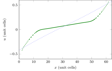
Figure 3: The standard conjugate gradient method at times $10$, $20$ and $30$ as shown by the solid, dashed and dotted lines, respectively. The block solidifies entirely while the deformation field is left practically unchanged. The blue dotted line shows the deformation field after $3000$ time units.

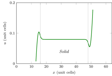
Figure 4: Deformation field of the initial setting seen in Fig. 2 after elastic equilibration.

The elastic equilibration through the conjugate gradient dynamics is very slow. It takes thousands of time units to get the equally strained deformation profile in Fig. 3 while it took only $39$ time units for the system to solidify. The solidification process with the elastic equilibrium imposed took only $19$ time units to solidify implying that even the dynamics of the $\phi$ field are different depending on whether the dynamics is solved in elastic equilibrium or not. The deformation field after the initial equilibration is shown in Fig. 4. The profile is simply stretched while the solid block grows.

V.3 Grain rotation in two dimensions

The elastic equilibration was also tested for the well known grain rotation phenomena Wu and Voorhees (2012); Cahn and Taylor (2004); Cahn et al. (2006) in a two-dimensional triangular system. In these simulations a circular grain is initially rotated by a certain angle $\alpha$ creating dislocations at the boundary between the circular grain and the surrounding solid body.

The classical description of grain boundary evolution states that the normal velocity of the grain boundary is proportional to its curvature. In the case of a circular grain the curvature can be written as $R(t)^{-1}$, where $R(t)$ is the radius of the circle. Now, $d/dt[R(t)]\sim R(t)^{-1}$, which implies that $d/dt[R(t)^{2}]$ is a constant. In other words, the area of the circular grain decreases linearly. The shrinking in the normal direction of the boundary ensures that shrinking of a circular grain is self similar, only the radius decreases.

Another consequence of the initial rotation is the rotation of the grain while shrinking. This is due to the fact that for small rotation angles the number of dislocations $n_{D}$ is conserved throughout the shrinking (until a rapid final collapse of the grain) and is proportional to the mismatch given by the rotation angle $\alpha(t)$ times the grain boundary length $2\pi R(t)$ i.e. $n_{D}\sim R(t)\alpha(t)$. This implies that $\alpha(t)\sim R(t)^{-1}$, which makes the rotation angle grow as the grain radius shrinks.

To examine this phenomena we first conducted a set of simulations with parameters identical to the ones chosen by Wu and Voorhees Wu and Voorhees (2012) who examined grain rotation using the PFC model, i.e., Eq. (2). A second set of simulations were also conducted for parameters in which the difference between the standard conjugate and the instantaneous elastic relaxation approaches is large.

The parametrisation of Wu and Voorhees Wu and Voorhees (2012) in our notation reads $\Delta B=-0.014075$, $B^{x}=1$, $\tau=0.585$ and $v=1$ and is from now on referred to as the warm case (parametrization). We calculated the dynamics also with a colder effective temperature by dropping the value of $\Delta B$ to $-0.05$ (cold parametrization). In both of these cases the initial rotation angle was chosen to be 5° corresponding to calculations done in Wu and Voorhees (2012). All the calculations were performed using isotropic spatial discretisation of $4.0$ and a time step of $1.0$. A simulation box of 1568$\times$1568 with periodic boundaries was used for all calculations. This comprises about 216$\times$216 atoms of which the rotated grain occupies about 1/4 with a diameter of 100 atoms.

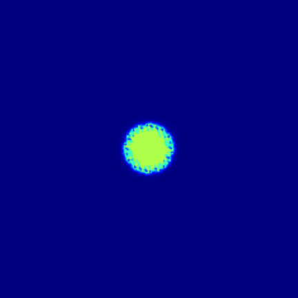
Figure 5: The norm of the gradient of the deformation field $\lVert\nabla\vec{u}\rVert$. Panels (a)-(c) show the time evolutions for warm parametrisation of Wu et al. Wu and Voorhees (2012) at times $10000$, $400000$, and $680000$, respectively. Brighter color stands for greater value of the norm. The dots on the perimeter show the dislocations at the grain boundary.

Fig. 5 shows the gradient of the deformation field $\lVert\nabla\vec{u}\rVert=\sqrt{\sum_{i,j}(\partial_{i}u_{j})^{2}}$ without the equilibration. For small angles this is proportional to the rotation angle inside the circle since the deformation is a pure rotation. The brighter colours at the boundary show the dislocations that join in the last panel to vanish shortly afterwards. It must be noted that the grain is shown in the original coordinates without any displacement. The radius and the angle as a function of time for the warm parametrisation can be seen in Fig. 6. These results agree very well with those in Ref. Wu and Voorhees (2012) and show that for this set of parameters the amplitude representation, i.e., Eq. (4) accurately reproduces the full PFC results, i.e., Eq. (2).

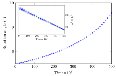
Figure 6: Angle of the shrinking grain for the warm parametrisation. Inset shows the corresponding squared radius.

For the warm case the dynamics with elastic equilibration is indistinguishable within the errors from the standard conjugate gradient dynamics. This is due to the fact that the parameters were chosen very close to the liquid state to avoid getting stuck at local energy minima. The elastic energies are very small close to the liquid state and the equilibration does not make any discernible difference. A linear fit to the squared radius data gives a slope of $-0.181\pm 0.01$ in dimensionless units.

The situation is very different in the cold case. Linear scaling of the squared radius still holds for both the equilibrated and the standard conjugate gradient dynamics, but the time scales are completely different as seen in Fig. 7. The slope of the linear fit to the squared radius data is $-0.157\pm 0.01$ for the cold case with conjugate gradient dynamics implying that the dynamics is slightly faster with the warm parametrisation as expected. The corresponding slope of the linear fit for the equilibrated dynamics in the cold case is $-1.47\pm 0.1$ that is almost ten times faster than the slope with the conjugate gradient dynamics. This suggests that with the standard conjugate gradient dynamics the inability to quickly reach elastic equilibrium severely hinders shrinkage.

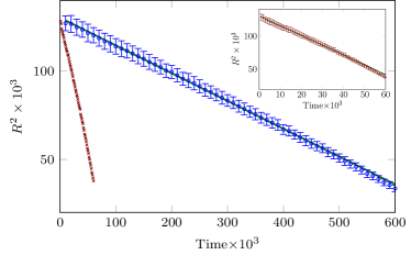
Figure 7: The steep line with the red crosses shows the squared radius data for the cold parametrisation with the elastic equilibration while the circles show the equivalent data for the standard conjugate gradient dynamics. The inset shows the data for the equilibrated dynamics with error bars.

VI Summary and Conclusions

We have proposed a method to separately relax elastic excitations in the amplitude expansion picture of the PFC model during non-conserved dissipative dynamics. This approach is shown to be consistent in the small deformation limit with the theory of linear elasticity. The numerical tests suggest that the approach indeed relaxes elastic excitations and furthermore that this relaxation can considerably change the dynamics.

An interesting result of the test cases is that the elastic excitations are extremely resilient in the diffusive time scales. It seems that the system tends to prefer solidification to relaxing simple elastic stretches and strains. This is unfortunate especially with systems driven out of equilibrium. Traditional conjugate gradient dynamics allows only for diffusive transportation of the information of any strains in the solid body. This is in conflict with the theory of elasticity that predicts ballistic transport of small displacements. This problem is present both in the PFC dynamics and the conjugate gradient dynamics of the amplitude expansion model, and becomes even more important when the system is mechanically driven out of equilibrium. Our approach to equilibrate the elastic excitations remedies this inherent shortcoming in the standard diffusive dynamics.

Appendix A Elastic excitations in bcc crystals

A.1 Elastic equilibrium from energy

To describe the bcc lattice first mode approximation we use the following reciprocal lattice vectors

$$\begin{split}&\vec{q}_{1}=(1,1,0)/\sqrt{2},\\ &\vec{q}_{2}=(1,0,1)/\sqrt{2},\\ &\vec{q}_{3}=(0,1,1)/\sqrt{2},\\ &\vec{q}_{4}=(0,1,-1)/\sqrt{2},\\ &\vec{q}_{5}=(1,-1,0)/\sqrt{2},\\ &\vec{q}_{6}=(-1,0,1)/\sqrt{2}.\\ \end{split}$$

The complete energy for a 3D bcc system is written down in Elder et al. (2010). As for the 2D case, the only term giving rise to elastic energy in the energy is again the term

$$4B^{x}\phi^{2}\sum_{k,l}q_{jk}q_{jl}(\partial_{k}\theta_{j})(\partial_{l}\theta_{j}),$$ (45)

and the elastic part of the energy can be defined as

$$F_{el}=\int_{\Omega}d\vec{r}\left[4B^{x}\phi^{2}\sum_{k,l,j}q_{jk}q_{jl}(\partial_{k}\theta_{j})(\partial_{l}\theta_{j})\right].$$ (46)

This in terms of the linear strain tensor is

$$\begin{split}F_{el}&=\int_{\Omega}d\vec{r}\left[8B^{x}\phi^{2}\left(2\sum_{i=1}^{3}\varepsilon_{ii}^{2}+4\varepsilon_{12}^{2}+4\varepsilon_{13}^{2}\right.\right.\\ &\left.\left.+4\varepsilon_{23}^{2}+2\varepsilon_{22}\varepsilon_{33}+2\varepsilon_{11}\varepsilon_{22}+2\varepsilon_{11}\varepsilon_{33}\vphantom{\sum_{i=1}^{3}}\right)\right].\end{split}$$ (47)

Now the stress tensor becomes

$$\begin{split}\sigma_{ii}&=\frac{\delta F_{el}}{\delta\varepsilon_{ii}}\\ &=32B^{x}\phi^{2}\varepsilon_{ii}+16B^{x}\phi^{2}\varepsilon_{jj}+16B^{x}\phi^{2}\varepsilon_{kk},\end{split}$$ (48)

for $i$, $j$, $k$ different and

$$\sigma_{ij}=\frac{1}{2}\frac{\delta F_{el}}{\delta\varepsilon_{ij}}=32B^{x}\phi^{2}\varepsilon_{ij},$$ (49)

for $i\neq j$. Writing the elastic equilibrium $\sum_{j}\partial_{j}\sigma_{ij}=0$ in terms of the components of $\vec{u}$ gives

$$2\partial_{i}^{2}u_{i}+(\partial_{j}^{2}+\partial_{k}^{2})u_{i}+2\partial_{i}(\partial_{j}u_{j}+\partial_{k}u_{k})=0,$$ (50)

for all $i$, $j$, $k$ different.

The elastic constants of the cubic crystal symmetry can be obtained as

$$\sigma_{ii} =C_{11}\varepsilon_{ii}+C_{12}(\varepsilon_{jj}+\varepsilon_{kk}),\quad\textrm{$i$, $j$, $k$ different;}$$ (51)

$$\sigma_{ij} =2C_{44}\varepsilon_{ij},\quad\textrm{$i\neq j$}$$ (52)

giving $C_{11}=32B^{x}\phi^{2}$, $C_{12}=16B^{x}\phi^{2}$ and $C_{44}=16B^{x}\phi^{2}$.

A.2 Elastic equilibrium from dynamics

The equivalent of Eq. (4) can be found from Elder et al. (2010). The dynamical equations of motion for $\phi$ are

$$\vec{q}_{j}\cdot\nabla\nabla^{2}\theta_{j}=c_{j},$$ (53)

where $c_{j}$ are constants. We will now combine different components of Eq. (53): $(j=1)+(j=5)$, $(j=2)+(j=6)$, $(j=1)-(j=5)$, $(j=2)-(j=6)$, $(j=3)-(j=4)$ and finally $(j=3)+(j=4)$, respectively, yield the following relations,

$$\begin{split}&(\partial_{1}^{3}+\partial_{1}\partial_{2}^{2}+\partial_{1}\partial_{3}^{2})u_{1}\\ +&(\partial_{2}\partial_{1}^{2}+\partial_{2}\partial_{3}^{2}+\partial_{2}^{3})u_{2}=d_{1},\end{split}$$ (54)

$$\begin{split}&(\partial_{1}^{3}+\partial_{1}\partial_{2}^{2}+\partial_{1}\partial_{3}^{2})u_{1}\\ +&(\partial_{3}\partial_{1}^{2}+\partial_{3}\partial_{2}^{2}+\partial_{3}^{3})u_{3}=d_{2},\end{split}$$ (55)

$$\begin{split}&(\partial_{1}^{3}+\partial_{1}\partial_{2}^{2}+\partial_{1}\partial_{3}^{2})u_{2}\\ +&(\partial_{2}\partial_{1}^{2}+\partial_{2}\partial_{3}^{2}+\partial_{2}^{3})u_{1}=d_{3},\end{split}$$ (56)

$$\begin{split}&(\partial_{1}^{3}+\partial_{1}\partial_{2}^{2}+\partial_{1}\partial_{3}^{2})u_{3}\\ +&(\partial_{3}\partial_{1}^{2}+\partial_{3}\partial_{2}^{2}+\partial_{3}^{3})u_{1}=d_{4},\end{split}$$ (57)

$$\begin{split}&(\partial_{2}^{3}+\partial_{2}\partial_{1}^{2}+\partial_{2}\partial_{3}^{2})u_{3}\\ +&(\partial_{3}\partial_{1}^{2}+\partial_{3}\partial_{2}^{2}+\partial_{3}^{3})u_{2}=d_{5},\end{split}$$ (58)

$$\begin{split}&(\partial_{2}^{3}+\partial_{2}\partial_{1}^{2}+\partial_{2}\partial_{3}^{2})u_{2}\\ +&(\partial_{3}\partial_{1}^{2}+\partial_{3}\partial_{2}^{2}+\partial_{3}^{3})u_{3}=d_{6},\end{split}$$ (59)

where $d_{j}$ are constants. Now, $\frac{1}{2}\partial_{1}$[Eq. (54)+Eq. (55)] $-\frac{3}{2}\partial_{1}$[Eq. (59)] $+\partial_{2}$[Eq. (56)] $+\partial_{3}$[Eq. (57)] gives

$$\nabla^{4}u_{1}=0.$$ (60)

Furthermore, $\partial_{1}$[Eq. (56)] $+\partial_{3}$[Eq. (58)] $+\frac{1}{2}\partial_{2}$ [Eq. (54) + Eq. (59)] $-\frac{3}{2}\partial_{2}$[Eq. (55)] yields

$$\nabla^{4}u_{2}=0.$$ (61)

Finally, from $\partial_{1}$[Eq. (57)] $+\partial_{2}$[Eq. (58)] $-\frac{3}{2}\partial_{3}$ [Eq. (54)] $+\frac{1}{2}\partial_{3}$[Eq. (55) + Eq. (59)], it follows that

$$\nabla^{4}u_{3}=0.$$ (62)

Thus, $\nabla^{4}\theta_{j}=0$.

The time evolution for the $\theta_{j}$ fields can be written as

$$\frac{d\theta_{j}}{dt}=-B^{x}\nabla^{4}\theta_{j}+4B^{x}\left(\vec{q}_{j}\cdot\nabla\right)^{2}\theta_{j},$$ (63)

which now simplifies into

$$\frac{d\theta_{j}}{dt}=4B^{x}\left(\vec{q}_{j}\cdot\nabla\right)^{2}\theta_{j}=4B^{x}\left(\vec{q}_{j}\cdot\nabla\right)^{2}\vec{q}_{j}\cdot\vec{u}.$$ (64)

The elastic equilibrium equations are written down with the help of Eq. (40) as

$$\sum_{j=1}^{6}\vec{q}_{j}\frac{d\theta_{j}}{dt}=0.$$ (65)

This becomes

$$\frac{d\theta_{1}}{dt}+\frac{d\theta_{2}}{dt}+\frac{d\theta_{5}}{dt}-\frac{d\theta_{6}}{dt} =0;$$ (66)

$$\frac{d\theta_{1}}{dt}+\frac{d\theta_{3}}{dt}+\frac{d\theta_{4}}{dt}-\frac{d\theta_{5}}{dt} =0;$$ (67)

$$\frac{d\theta_{2}}{dt}+\frac{d\theta_{3}}{dt}-\frac{d\theta_{4}}{dt}+\frac{d\theta_{6}}{dt} =0.$$ (68)

The time derivatives can be replaced using Eq. (64) giving

$$2\partial_{1}^{2}u_{1}+\partial_{2}^{2}u_{1}+\partial_{3}^{2}u_{1}+2\partial_{1}\partial_{2}u_{2}+2\partial_{1}\partial_{3}u_{3} =0;$$ (69)

$$2\partial_{2}^{2}u_{2}+\partial_{1}^{2}u_{2}+\partial_{3}^{2}u_{2}+2\partial_{1}\partial_{2}u_{1}+2\partial_{2}\partial_{3}u_{3} =0;$$ (70)

$$2\partial_{3}^{2}u_{3}+\partial_{1}^{2}u_{3}+\partial_{2}^{2}u_{3}+2\partial_{1}\partial_{3}u_{1}+2\partial_{2}\partial_{3}u_{2} =0,$$ (71)

which give $\left(\nabla\cdot\sigma\right)_{i}=0$ for $i=1,2,3$ respectively.

Appendix B Elastic excitations in fcc crystals

In order to reproduce the fcc lattice symmetry, two different sets of reciprocal lattice vectors of different scales are needed (two-mode approximation) that are both cubically symmetric. Let us choose them to be

$$\begin{split}&\vec{q}_{1}=(-1,1,1)/\sqrt{3},\\ &\vec{q}_{2}=(1,-1,1)/\sqrt{3},\\ &\vec{q}_{3}=(1,1,-1)/\sqrt{3},\\ &\vec{q}_{4}=(-1,-1,-1)/\sqrt{3},\\ &\vec{q}_{5}=2(0,0,1)/\sqrt{3},\\ &\vec{q}_{6}=2(1,0,0)/\sqrt{3},\\ &\vec{q}_{7}=2(0,1,0)/\sqrt{3}.\\ \end{split}$$

B.1 Elastic equilibrium from the energy

Full energy for the fcc system can be found from Ref. Elder et al. (2010). Again, the only term giving rise to elastic energy in the energy is the term

$$4B^{x}\phi^{2}\sum_{k,l}q_{jk}q_{jl}(\partial_{k}\theta_{j})(\partial_{l}\theta_{j}),$$ (72)

and the elastic part of the energy can be defined as

$$F_{el}=\int_{\Omega}d\vec{r}\left[4B^{x}\phi^{2}\sum_{k,l,j}q_{jk}q_{jl}(\partial_{k}\theta_{j})(\partial_{l}\theta_{j})\right].$$ (73)

This in terms of the linear strain tensor is

$$\begin{split}F_{el}&=\int_{\Omega}d\vec{r}\left[16B^{x}\phi^{2}\left(5\sum_{i=1}^{3}\varepsilon_{ii}^{2}+4\varepsilon_{12}^{2}+4\varepsilon_{13}^{2}\right.\right.\\ &\left.\left.+4\varepsilon_{23}^{2}+2\varepsilon_{22}\varepsilon_{33}+2\varepsilon_{11}\varepsilon_{22}+2\varepsilon_{11}\varepsilon_{33}\vphantom{\sum_{i=1}^{3}}\right)\right].\end{split}$$ (74)

Now the stress tensor becomes

$$\begin{split}\sigma_{ii}&=\frac{\delta F_{el}}{\delta\varepsilon_{ii}}\\ &=160B^{x}\phi^{2}\varepsilon_{ii}+32B^{x}\phi^{2}\varepsilon_{jj}+32B^{x}\phi^{2}\varepsilon_{kk},\end{split}$$ (75)

for all $i$, $j$, $k$ different and

$$\sigma_{ij}=\frac{1}{2}\frac{\delta F_{el}}{\delta\varepsilon_{ij}}=64B^{x}\phi^{2}\varepsilon_{ij},$$ (76)

for all $i\neq j$. Writing the elastic equilibrium $\sum_{j}\partial_{j}\sigma_{ij}=0$ in terms of the components of $\vec{u}$ gives

$$5\partial_{i}^{2}u_{i}+(\partial_{j}^{2}+\partial_{k}^{2})u_{i}+2\partial_{i}(\partial_{j}u_{j}+\partial_{k}u_{k})=0,$$ (77)

for all $i$, $j$, $k$ different.

The elastic constants are again from the cubic crystal symmetry

$$\sigma_{ii} =C_{11}\varepsilon_{ii}+C_{12}(\varepsilon_{jj}+\varepsilon_{kk}),\quad\textrm{$i$, $j$, $k$ different};$$ (78)

$$\sigma_{ij} =2C_{44}\varepsilon_{ij},\quad\textrm{$i\neq j$}.$$ (79)

Now $C_{11}=160B^{x}\phi^{2}$, $C_{12}=32B^{x}\phi^{2}$ and $C_{44}=32B^{x}\phi^{2}$.

B.2 Elastic equilibrium from dynamics

The evolution of the complex amplitudes can be found from Ref. Elder et al. (2010). When making again the assumption that $\eta_{j}=\phi_{j}e^{i\vec{q}_{j}\cdot\vec{u}}$ with constant $\phi_{j}$ and going to linear order in $\vec{u}$ gives us equation for the amplitudes as

$$\sum_{k,l}q_{jk}\partial_{k}v_{l}q_{jl}=C_{1},$$ (80)

for $j=1,2,3,4$ and

$$\sum_{k,l}q_{jk}\partial_{k}v_{l}q_{jl}=C_{2},$$ (81)

for $j=5,6,7$. Here $C_{1}$ and $C_{2}$ are constants consisting of constant amplitudes and model parameters and $\vec{v}=\nabla^{2}\vec{u}$. Again we need to show that the biharmonic equation $\nabla^{4}\vec{u}$ follows. Inserting the reciprocal vectors $\vec{q}_{5}$, $\vec{q}_{6}$, and $\vec{q}_{7}$ in Eq. (81) gives

$$\partial_{i}v_{i}=C_{2},$$ (82)

for all $i$.

Next, let us open Eq. (80)

$$\begin{split}&q_{j1}^{2}\partial_{1}v_{1}+q_{j2}^{2}\partial_{2}v_{2}+q_{j3}^{2}\partial_{3}v_{3}\\ &+q_{j1}q_{j2}(\partial_{1}v_{2}+\partial_{2}v_{1})+q_{j1}q_{j3}(\partial_{1}v_{3}+\partial_{3}v_{1})\\ &+q_{j2}q_{j3}(\partial_{2}v_{3}+\partial_{3}v_{2})=C_{2}.\end{split}$$ (83)

We can take advatage of the fact that the set $\{\vec{q}_{j}\}$ is invariant under cubic symmetry operations. Using reflections of the coordinate $i$ and subtracting from both sides of (83) it follows that

$$q_{ji}q_{jk}(\partial_{i}v_{k}+\partial_{k}v_{i})+q_{ji}q_{jl}(\partial_{i}v_{l}+\partial_{l}v_{i})=0,$$ (84)

or

$$q_{jk}(\partial_{i}v_{k}+\partial_{k}v_{i})+q_{jl}(\partial_{i}v_{l}+\partial_{l}v_{i})=0,$$ (85)

since $q_{ji}$ are non-zero for $i=1,2,3,4$. Here the indices $i$, $k$, $l$ are all different so Eq. (85) applies for all the permutations of $1$, $2$ and $3$. Using reflection on $q_{jl}$ and adding to Eq. (85) gives

$$q_{jk}(\partial_{i}v_{k}+\partial_{k}v_{i})=0,$$ (86)

or

$$(\partial_{i}v_{k}+\partial_{k}v_{i})=0,$$ (87)

for all $k\neq i$. Taking derivative $\partial_{i}$ it follows that

$$\partial_{i}^{2}v_{k}=0,$$ (88)

since $\partial_{k}\partial_{i}v_{i}=0$ according to Eq. (82). Now

$$(\partial_{1}^{2}+\partial_{2}^{2}+\partial_{3}^{2})v_{i}=0,$$ (89)

for all $i$ i.e. $\nabla^{4}\vec{u}=0$.

The time evolution for $\theta_{j}$ after applying the biharmonic equation becomes

$$\frac{d\theta_{j}}{dt}=4B^{x}(\vec{q}_{j}\cdot\vec{\nabla})^{2}\vec{q}_{j}\cdot\vec{u},$$ (90)

or in terms of components

$$\frac{d\theta_{j}}{dt}=4B^{x}\sum_{k,l,p}q_{jk}q_{jl}\partial_{k}\partial_{l}q_{jp}u_{p},$$ (91)

for all $i=1-7$.

The elastic equilibrium condition can be written down using Eq. (40) as

$$\sum_{j=1}^{7}\vec{q}_{j}\frac{d\theta_{j}}{dt}=0,$$ (92)

giving

$$-\frac{d\theta_{1}}{dt}+\frac{d\theta_{2}}{dt}+\frac{d\theta_{3}}{dt}-\frac{d\theta_{4}}{dt}+2\frac{d\theta_{6}}{dt} =0;$$ (93)

$$\frac{d\theta_{1}}{dt}-\frac{d\theta_{2}}{dt}+\frac{d\theta_{3}}{dt}-\frac{d\theta_{4}}{dt}+2\frac{d\theta_{7}}{dt} =0;$$ (94)

$$\frac{d\theta_{1}}{dt}+\frac{d\theta_{2}}{dt}-\frac{d\theta_{3}}{dt}-\frac{d\theta_{4}}{dt}+2\frac{d\theta_{5}}{dt} =0.$$ (95)

Using Eq. (91) this gives

$$5\partial_{1}^{2}u_{1}+(\partial_{2}^{2}+\partial_{3}^{2})u_{1}+2\partial_{1}(\partial_{2}u_{2}+\partial_{3}u_{3}) =0;$$ (96)

$$5\partial_{2}^{2}u_{2}+(\partial_{1}^{2}+\partial_{3}^{2})u_{2}+2\partial_{2}(\partial_{1}u_{1}+\partial_{3}u_{3}) =0;$$ (97)

$$5\partial_{3}^{2}u_{3}+(\partial_{1}^{2}+\partial_{2}^{2})u_{3}+2\partial_{3}(\partial_{1}u_{1}+\partial_{2}u_{2}) =0,$$ (98)

which constitutes to $(\nabla\cdot\sigma)_{i}=0$ for indices $i=1,2,3$, respectively i.e. gives the elastic equilibrium condition.

Appendix C Elastic excitations in 1D

C.1 Separation of complex amplitudes

Energy for a 1D system can be written as

$$F_{1D}=\int_{\Omega}dx[\Delta B|\eta|^{2}+B^{x}|\mathcal{G}\eta|^{2}+\frac{3}{2}v|\eta|^{4}],$$ (99)

where $\mathcal{G}=\partial_{x}^{2}+2i\partial_{x}$. The time evolution for $\eta$ is

$$\begin{split}\frac{d\eta}{dt}&=-\frac{\delta E_{1D}}{\delta\eta^{*}}=\frac{d\phi}{dt}e^{i\theta}+i\phi\frac{d\theta}{dt}e^{i\theta}\\ &=-\left\{\Delta B\eta+B^{x}\mathcal{G}^{2}\eta+3v|\eta|^{2}\eta\right\}.\end{split}$$ (100)

Opening the right-hand side and separating the complex and the real parts gives

$$\begin{split}\frac{d\phi}{dt}&=-\Delta B\phi\\ &-B^{x}[4\phi(\partial_{x}\theta)^{2}+4\phi(\partial_{x}\theta)^{3}+\phi(\partial_{x}\theta)^{4}\\ &-12(\partial_{x}\phi)(\partial_{x}^{2}\theta)-12(\partial_{x}\theta)(\partial_{x}\phi)(\partial_{x}^{2}\theta)\\ &-3\phi(\partial_{x}^{2}\theta)^{2}-4\partial_{x}^{2}\phi-12(\partial_{x}\theta)(\partial_{x}^{2}\phi)\\ &-6(\partial_{x}\theta)^{2}(\partial_{x}^{2}\phi)-4\phi(\partial_{x}^{3}\theta)\\ &-4\phi(\partial_{x}\theta)(\partial_{x}^{3}\theta)+\partial_{x}^{4}\phi]-3v\phi^{3},\end{split}$$ (101)

and

$$\begin{split}\phi\frac{d\theta}{dt}&=-B^{x}[-8(\partial_{x}\theta)(\partial_{x}\phi)-12(\partial_{x}\theta)^{2}(\partial_{x}\phi)\\ &-4(\partial_{x}\theta)^{3}(\partial_{x}\phi)-4(\partial_{x}^{2}\theta)\phi\\ &-12\phi(\partial_{x}\theta)(\partial_{x}^{2}\theta)-6(\partial_{x}\theta)^{2}(\partial_{x}^{2}\theta)\phi\\ &+6(\partial_{x}^{2}\theta)(\partial_{x}^{2}\phi)+4(\partial_{x}^{3}\theta)(\partial_{x}\phi)\\ &+4(\partial_{x}^{3}\phi)+4(\partial_{x}\theta)(\partial_{x}^{3}\phi)+(\partial_{x}^{4}\theta)\phi].\end{split}$$ (102)

In one dimension the deformation field $u=\theta$, which gives an expression for the elastic equilibrium condition

$$\frac{d\theta}{dt}=0.$$ (103)

C.2 Linear elasticity

Let us consider evolution of $\phi$ given by Eq. (101). Writing $\theta(x)=u(x)$ and going to linear order in the deformation field $u$ gives an equation for constant $\phi$

$$\partial_{x}^{3}u=\frac{\Delta B+3v\phi^{2}}{4B^{x}}=C,$$ (104)

where $C=\textit{const.}$, from which it follows that

$$\partial_{x}^{4}u=0.$$ (105)

Writing down the condition of Eq. (103) for Eq. (102) in the linear regime gives

$$-4\partial_{x}^{2}u+\partial_{x}^{4}u=0,$$ (106)

implying that

$$\partial_{x}^{2}u=0.$$ (107)

The same relation follows in the linear elasticity limit from the energy by taking the functional derivative with respect to the deformation field i.e. demanding that

$$\frac{\delta F_{1D}}{\delta u}=\frac{\delta F_{1D}}{\delta\theta}=0.$$ (108)

References

• Elder et al. (2002) K. R. Elder, M. Katakowski, M. Haataja, and M. Grant, Phys. Rev. Lett. 88, 245701 (2002).
• Elder and Grant (2004) K. R. Elder and M. Grant, Phys. Rev. E 70, 051605 (2004).
• Elder et al. (2007) K. R. Elder, N. Provatas, J. Berry, P. Stefanovic, and M. Grant, Phys. Rev. B 75, 064107 (2007).
• Berry et al. (2008a) J. Berry, K. R. Elder, and M. Grant, Phys. Rev. B 77 (2008a).
• Mellenthin et al. (2008) J. Mellenthin, A. Karma, and M. Plapp, Phys. Rev. B 78 (2008).
• Jaatinen et al. (2009) A. Jaatinen, C. Achim, K. R. Elder, and T. Ala-Nissila, Phys. Rev. E 80, 031602 (2009).
• Tegze et al. (2011) G. Tegze, G. I. Tóth, and L. Gránásy, Phys. Rev. Lett. 106 (2011).
• Achim et al. (2006) C. Achim, M. Karttunen, K. R. Elder, E. Granato, T. Ala-Nissila, and S. Ying, Phys. Rev. E 74 (2006).
• Achim et al. (2009) C. Achim, J. Ramos, M. Karttunen, K. R. Elder, E. Granato, T. Ala-Nissila, and S. Ying, Phys. Rev. E 79 (2009).
• Ramos et al. (2010) J. A. P. Ramos, E. Granato, S. C. Ying, C. V. Achim, K. R. Elder, and T. Ala-Nissila, Phys. Rev. E 81, 011121 (2010).
• Ramos et al. (2008) J. Ramos, E. Granato, C. Achim, S. Ying, K. R. Elder, and T. Ala-Nissila, Phys. Rev. E 78 (2008).
• Wu and Voorhees (2009) K.-A. Wu and P. W. Voorhees, Phys. Rev. B 80, 125408 (2009).
• Stefanovic et al. (2006) P. Stefanovic, M. Haataja, and N. Provatas, Phys. Rev. Lett. 96 (2006).
• Hirouchi et al. (2009) T. Hirouchi, T. T, and T. Tomita, Comput. Mat. Sci. 44, 1192 (2009).
• Stefanovic et al. (2009) P. Stefanovic, M. Haataja, and N. Provatas, Phys. Rev. E 80 (2009).
• Berry et al. (2008b) J. Berry, K. R. Elder, and M. Grant, Phys. Rev. E 77, 061506 (2008b).
• Berry and Grant (2011) J. Berry and M. Grant, Phys. Rev. Lett. 106, 175702 (2011).
• Marconi and Tarazona (1999) U. Marconi and P. Tarazona, J. Chem. Phys. 110, 8032 (1999).
• Archer and Evans (2004) A. J. Archer and R. Evans, J. Chem. Phys. 121, 4246 (2004).
• Majaniemi and Grant (2007) S. Majaniemi and M. Grant, Phys. Rev. B 75, 054301 (2007).
• Goldenfeld et al. (2005) N. Goldenfeld, B. Athreya, and J. Dantzig, Phys. Rev. E 72, 020601 (2005).
• Athreya et al. (2006) B. Athreya, N. Goldenfeld, and J. Dantzig, Phys. Rev. E 74, 011601 (2006).
• Goldenfeld et al. (2006) N. Goldenfeld, B. P. Athreya, and J. A. Dantzig, J. Stat. Phys. 125, 1015 (2006).
• Elder et al. (2010) K. R. Elder, Z.-F. Huang, and N. Provatas, Phys. Rev. E 81, 011602 (2010).
• Huang et al. (2010) Z.-F. Huang, K. R. Elder, and N. Provatas, Phys. Rev. E 82, 021605 (2010).
• Yeon et al. (2010) D.-E. Yeon, Z.-F. Huang, K. R. Elder, and K. Thornton, Phil. Mag. 90, 237 (2010).
• Athreya et al. (2007) B. Athreya, N. Goldenfeld, J. Dantzig, M. Greenwood, and N. Provatas, Phys. Rev. E 76 (2007).
• Huang and Elder (2008) Z.-F. Huang and K. R. Elder, Phys. Rev. Lett. 101, 158701 (2008).
• Huang and Elder (2010) Z.-F. Huang and K. R. Elder, Phys. Rev. B 81, 364103 (2010).
• Elder et al. (2012) K. R. Elder, G. Rossi, P. Kanerva, F. Sanches, S.-C. Ying, E. Granato, C. V. Achim, and T. Ala-Nissila, Phys. Rev. Lett. 108, 226102 (2012).
• Elder et al. (2013) K. R. Elder, G. Rossi, P. Kanerva, F. Sanches, S.-C. Ying, E. Granato, C. V. Achim, and T. Ala-Nissila, Phys. Rev. B 88, 075423 (2013).
• Muller and Grant (1999) J. Muller and M. Grant, Phys. Rev. Lett. 82, 035401 (1999).
• Haataja et al. (2002) M. Haataja, J. Muller, A. D. Rutenberg, and M. Grant, Phys. Rev. B 65, 035401 (2002).
• Orlikowski et al. (1999) D. Orlikowski, C. Sagui, A. Somoza, and C. Roland, Phys. Rev. B 59, 8646 (1999).
• Wang et al. (2001) Y. U. Wang, Y. M. Jin, A. M. Cuitino, and A. G. Khachaturyan, Appl. Phys. Lett. 63, 224114 (2001).
• Landau et al. (1986) L. Landau, E. Lifshitz, A. Kosevitch, and L. Pitaevskiĭ, Theory of Elasticity, Course of theoretical physics (Butterworth-Heinemann, Oxford, 1986), ISBN 9780750626330.
• Wu and Voorhees (2012) K.-A. Wu and P. W. Voorhees, Acta Mater. 60, 407 (2012).
• Cahn and Taylor (2004) J. W. Cahn and J. E. Taylor, Acta Mater. 52, 4887 (2004).
• Cahn et al. (2006) J. W. Cahn, Y. Mishin, and A. Suzuki, Phil. Mag. 86, 3965 (2006).