Logistic regression analysis with standardized markers

Abstract

Two different approaches to analysis of data from diagnostic biomarker studies are commonly employed. Logistic regression is used to fit models for probability of disease given marker values, while ROC curves and risk distributions are used to evaluate classification performance. In this paper we present a method that simultaneously accomplishes both tasks. The key step is to standardize markers relative to the nondiseased population before including them in the logistic regression model. Among the advantages of this method are the following: (i) ensuring that results from regression and performance assessments are consistent with each other; (ii) allowing covariate adjustment and covariate effects on ROC curves to be handled in a familiar way, and (iii) providing a mechanism to incorporate important assumptions about structure in the ROC curve into the fitted risk model. We develop the method in detail for the problem of combining biomarker data sets derived from multiple studies, populations or biomarker measurement platforms, when ROC curves are similar across data sources. The methods are applicable to both cohort and case–control sampling designs. The data set motivating this application concerns Prostate Cancer Antigen 3 (PCA3) for diagnosis of prostate cancer in patients with or without previous negative biopsy where the ROC curves for PCA3 are found to be the same in the two populations. The estimated constrained maximum likelihood and empirical likelihood estimators are derived. The estimators are compared in simulation studies and the methods are illustrated with the PCA3 data set.

T1Supported by NIH Grants U01 CA086368-06, RO1 GM054438, PO1 CA053996, U24CA086368, and P30CA015704.

, and

1 Introduction

As myriads of biomarkers are becoming available from research laboratories, the demand for more sophisticated statistical analysis methods increases. For example, an emerging request is to combine information from multiple sources in evaluating a biomarker’s performance. In addition, biomarkers must be evaluated from multiple points of view, including, for example, their roles as risk factors and predictors as well as their classification performance.

Logistic regression analysis has been a mainstay of biostatistical methodology for evaluating risk factors, particularly in epidemiology and in therapeutic research. For evaluating biomarker performance, however, other methods are more appropriate, such as those based on receiver operating characteristic (ROC) curves [Pepe (2003)] and risk distributions. Methods that evaluate categorized risk distributions are gaining popularity and are often called risk reclassification methods. However, in general, methods for evaluating performance are far less well developed and have more limited availability than logistic regression methodology.

In this paper we show that evaluation of biomarker performance can be achieved within the logistic regression framework if as a preliminary step one standardizes the marker using the control population to define the reference distribution for standardization. Previously, in a simple setting with the biomarker as the only predictor of interest, Gu and Pepe (2010) applied a logistic regression model to standardized marker values as a rank-invariant approach to estimating the variance of the empirical ROC curve in sample size calculations. Here we extend the approach to estimate the ROC curve itself and to allow for additional covariates. Through recognition of the fact that there is a direct functional relationship between the coefficient for the standardized marker in the logistic regression model and the ROC curve, we show that risk distributions as well as the ROC curve conditional on covariates can be calculated directly from coefficients in the model and that incorporating this relationship into estimation leads to efficiency gains. Since the method simultaneously evaluates the marker as a risk factor and the marker’s performance as a classifier, it provides a more coherent approach than current methods that separately evaluate the two aspects. Potentially inconsistent results are avoided. The framework has several other attributes. First, estimated ROC curves can be constrained to be concave if desired. Concavity is a fundamental property of the ROC curve that is not taken advantage of by most standard methods. Second, covariate effects on biomarker performance can be addressed naturally within the logistic regression framework. Third, the method is rank invariant with respect to the marker, adding a degree of robustness compared with usual logistic regression.

The general framework and methods for estimation are presented in Section 2. The method is then developed in some detail for the problem of evaluating a biomarker using data derived from multiple studies or populations when a common ROC curve across data sources is of interest. This is an important problem for which methodology has not been proposed heretofore. Consider that prior to launching a large validation study, data from multiple small studies, possibly using different assay platforms, may be examined. Methods that can combine information across studies are needed in this setting. Moreover, when a large collaborative validation study is undertaken, it typically involves multiple sites that may each follow somewhat different protocols or involve multiple subpopulations that differ in regard to patient characteristics. Again, in this setting, our methods for combining data based on a common ROC curve will be useful. The example that motivated our work concerns evaluating a prostate cancer biomarker in two subpopulations of men.

In Section 3 we describe this example in detail and develop three methods for estimating parameters in the logistic regression model. We evaluate the properties of these estimators in simulation studies and describe results in Section 4. In Section 5 we illustrate the methodology using the data set from the prostate cancer biomarker study and finish with some concluding remarks in Section 6.

2 The general framework: Logistic regression applied to standardized biomarker values

2.1 The risk model is related to the ROC curve

Consider a binary outcome $D$, disease, say, with $D=0$ for control nondiseased subjects and $D=1$ for case diseased subjects, a single continuous marker $Y$, and additional covariates denoted by $X$. Note the marker $Y$ may be a predefined combination of predictors. For example, the Framingham risk score is a linear combination of risk factors for cardiovascular events including age, total cholesterol, and systolic blood pressure. Another example is the Oncotype-DX recurrence score that is a fixed combination of 21 gene expression assays. For an observation with marker measurement $Y=y$ and covariate value $X=x$, let the standardized marker value be $U=U(x,y)=P(Y>y|D=0,X=x)$. That is, using as a reference the marker distribution among controls with covariate value $x$, $U$ is the proportion of marker values in the reference distribution exceeding $y$. $U$ has been called the placement value for $Y$ [Pepe and Cai (2004)] and $100\times(1-U)$ is recognized as the percentile of $Y$ in the reference population [Hanley and Hajian-Tilaki (1997), Huang and Pepe (2009a)]. Percentiles are commonly used to standardize growth and lung function measurements for children and to standardize many laboratory measures. Note that the risk function can be written in terms of $Y$ or $U$, $P(D=1|Y,X)=P(D=1|U,X)$. Using the latter formulation, we propose the following logistic regression model:

$$\operatorname{logit}P(D=1|U,X)=\operatorname{logit}P(D=1|X)+G(U,X,\beta),$$ (1)

where $G(U,X,\beta)$ is some parametric function of $U$ and $X$ parameterized by $\beta$, and $\operatorname{logit}P(D=1|X)$ is an offset term that will be entered into the model before the application of the logistic regression.

Interestingly, we can show that $G(U,X,\beta)$ in this framework corresponds to the log-derivative of $\operatorname{ROC}_{X}$, where $\operatorname{ROC}_{x}$ is the ROC curve for $Y$ in the covariate specific population with $X=x$.

Theorem 1

Under model (1), $\operatorname{ROC}_{x}(t)=\int_{0}^{t}\exp\{G(u,x,\beta)\}\,du$ and $G(u,x,\beta)=\log\operatorname{ROC}_{x}^{\prime}(u)$.

A proof of Theorem 1 can be found in Appendix A of the supplementary material [Huang, Pepe and Feng (2013)]. The proposed framework (1) therefore naturally links risk modeling with ROC analysis. These two analytic tasks are typically undertaken separately in current practice, leading to disjointed and possibly inconsistent results, as illustrated in a simulated example in Appendix B of the supplementary material [Huang, Pepe and Feng (2013)]. Having a unified framework for risk modeling and for ROC analysis offers a more coherent approach to biomarker evaluation.

2.2 Ensuring concave ROC curves

An important attribute of this framework is that the ROC curve using the marker as the decision variable can be easily constrained to be concave if desired. Concavity is a fundamental characteristic of proper ROC curves [Egan (1975), Dorfman et al. (1996)]. In settings where it is reasonable to assume a monotone relationship between the risk of disease and the marker, the corresponding ROC curve for the marker is necessarily concave. Yet concavity has not been strictly enforced in ROC modeling. Indeed, the classic binormal ROC model that is widely used in radiology is not constrained to be concave. The binormal ROC curve assumes the existence of a common monotone transformation that transforms the marker distributions of cases and controls to normality, but if the variances of those normal distributions differ, the ROC curve is not concave. There have been several concave ROC models proposed in the literature, including the “bigamma” ROC curve [Dorfman et al. (1996)], the “bilomax” ROC curve [Campbell and Ratnaparkhi (1993)], and the “proper” binormal ROC curve [Metz and Pan (1999)]. Use of these models has been limited, however, partly due to difficulties in their implementation. In our framework (1), we model $G(u,x,\beta)$, the log-derivative of the ROC curve directly rather than modeling the ROC curve itself. Consequently, it is easy to constrain the ROC curve to be concave by modeling $G(u,x,\beta)$ as a monotone decreasing function of $u$.

2.3 Incorporating covariates

Equation (1) can be recognized as showing the association between the pre-test and post-test risk of disease where $G(U,X,\beta)$ is known as the covariate specific diagnostic likelihood ratio. Using Bayesian terminology, $G(U,X,\beta)$ is the Bayes factor that relates the prior and posterior probabilities of disease. However, very little methodology exists that exploits its relationship with the ROC curve, $G(U,X,\beta)=\log\operatorname{ROC}_{X}^{\prime}(U)$. To our knowledge, the only previous use of this framework is by Gu and Pepe (2010), who exploited a simplified version of (1) without covariates for a different problem of estimating the variance of the empirical ROC curve in sample size calculation.

The framework provides a mechanism to incorporate covariates $X$ into the model for the ROC curve through $G(U,X,\beta)=\log\operatorname{ROC}_{X}^{\prime}(U)$. This model provides opportunities for evaluating effects of covariates on the discriminatory power of the marker. To illustrate, consider the following toy example. Suppose $X$ is comprised of two subsets $X_{1}$ and $X_{2}$ that can each be multivariate, for example, $X_{1}=\mathrm{age}$ and $X_{2}=\mathrm{gender}$. Suppose we are interested in testing whether $X_{2}$ affects the marker’s classification accuracy. We model $G(U,X,\beta)$ as $\beta_{0}+\beta_{1}r(U)+\beta_{2}^{T}X_{1}+\beta_{3}^{T}X_{1}r(U)+\beta_{4}^{T}X_{2}+\beta_{5}^{T}X_{2}r(U)$, where $r(u)$ is some pre-specified function of $u$. Then the null hypothesis $H_{0}$, that $X_{2}$ does not affect the ROC curve, corresponds to zero coefficients for terms involving $X_{2}$, that is, $H_{0}\dvtx\beta_{4}=\beta_{5}=0$. The approach applies in general: we can test whether a subset of covariates affect the marker’s discriminatory accuracy by testing the corresponding coefficients in the risk model. One appealing property of (1) is that it naturally separates covariate effects for marker standardization from covariate effects for ROC analysis. Specifically, covariates used in deriving $U$ are those affecting the marker distribution in the control population, whereas covariates involved in $G(U,X,\beta)$ are those affecting the discriminatory power of the marker, as characterized by the ROC curve.

Two natural competing methods existing in the literature for covariate adjustment in ROC estimation using standardized marker values are the nonparametric ROC adjustment method proposed by Janes and Pepe (2008, 2009) and various semiparametric regression methods based on the binormal ROC model, such as the ROC-GLM method [Alonzo and Pepe (2002)] and the pseudo-likelihood method [Pepe and Cai (2004)]. Compared to the nonparametric method, applying a logistic regression form provides a much more efficient alternative. As mentioned in Section 2.2, existing semiparametric methods relying on the binormal ROC curve are not natural for modeling a concave ROC curve. In addition, as detailed in Sections 3 and 4, they make inference using standardized marker values among cases only, whereas the proposed method utilizes standardized marker values for all subjects and gains efficiency as a consequence.

2.4 Estimation

Consider first a cohort or cross-sectional study. Before fitting the logistic regression model to estimate regression coefficients, we first need to estimate the offset term $\operatorname{logit}P(D=1|X)$ and the standardized marker values $U$. Denote the estimators by $\hat{P}(D=1|X)$ and $\hat{U}$, respectively. For a cohort or cross-sectional study, $\hat{P}(D=1|X)$ can be derived in standard fashion using logistic regression techniques or nonparametrically if $X$ is discrete. Computation of $\hat{U}$ requires estimating the distribution of $Y$ in the control population conditional on $X$. Methods have been described and we refer to Huang and Pepe (2009a) for details. In particular, they suggest nonparametric methods for discrete $X$, and parametric and semiparametric methods for continuous $X$. After obtaining $\hat{P}(D=1|X)$ and $\hat{U}$, we substitute them into the logistic regression model (1) to estimate coefficients for $X$ and $\hat{U}$ using standard logistic regression fitting procedures including $\operatorname{logit}\hat{P}(D=1|X)$ as an offset term.

Consider a case–control sample where cases and controls are randomly sampled from the case and control subpopulations. Estimation of $U$ can be performed as in a cohort or cross-sectional study. Let $\mathit{Sampled}$ denote being sampled into the case–control set. According to Bayes’ theorem, we have

$$\frac{P(D=1|U,X)}{P(D=0|U,X}\frac{P(D=0|X)}{P(D=1|X)}$$

$$\qquad=\frac{P(D=1|U,X,\mathrm{Sampled})}{P(D=0|U,X,\mathrm{Sampled})}\frac{P(D=0|X,\mathrm{Sampled})}{P(D=1|X,\mathrm{Sampled})},$$

which implies that equation (1) can be written as

$$\operatorname{logit}P(D=1|U,X,\mathrm{Sampled})$$

$$\qquad=\operatorname{logit}P(D=1|X,\mathrm{Sampled})+G(U,X,\beta).$$

Thus, the estimate of regression coefficients for (1) can be obtained by applying an ordinary logistic regression to $D$, $X$, and $\hat{U}$ to the case–control sample with $\operatorname{logit}\hat{P}(D=1|X,\mathrm{Sampled})$ entered as an offset, where $\hat{P}(D=1|X,\mathrm{Sampled})$ is an estimate of $P(D=1|X,\mathrm{Sampled})$ based on the case–control sample.

After the model coefficients for (1) are obtained either based on a cohort, a cross-sectional, or a case–control sample, disease risk for each subject can be computed by entering $\hat{P}(D=1|X)$ and the individual’s $\hat{U}$ into the estimated model. For a case–control sample, in order to estimate $P(D=1|X)$, information about prevalence, $P(D=1)$, has to be acquired externally, for example, from the literature, from another independent cohort, or from the parent cohort within which the case–control sample is nested. For evaluation of a biomarker’s classification and prediction performance conditional on covariates, methods have been developed previously when the risk of disease conditional on the biomarker and covariates follows a logistic regression model [Huang, Pepe and Feng (2007), Huang and Pepe (2010a)]. These methods can be applied here, replacing the biomarker value on the original scale $Y$ with their estimated standardized value $\hat{U}$. Note that the $\hat{U}$’s are correlated with each other due to use of the control sample for estimating the reference distributions for standardization. Hence, standard variance formulae from logistic regression results do not apply, as they assume independence between observations. Additional complexity is also introduced by using an estimated offset term. Instead we propose bootstrap resampling for estimating variances of parameter estimators and constructing confidence intervals using percentiles of the bootstrap distribution. The resampling procedures need to mimic the design of the original study. Specifically, separate resampling of cases and controls would be warranted if the study is of case–control design, while for a cohort study resampling would be at random from the cohort without regard to outcome status.

3 Methodology for combining data sources through a common ROC curve

3.1 Combining data sets with common ROC curves

In the remainder of this manuscript, we focus on a specific problem where we evaluate biomarker performance combining data from multiple sources through estimation of a common ROC curve across data sources. The covariate $X$ characterizes the data source and we show how to use the logistic regression methodology to take advantage of the constraint that the ROC curves are common across $X$.

The study motivating this research is a cross-sectional study conducted by the Early Detection Research Network assessing a urine biomarker for prostate cancer, Prostate Cancer Antigen 3 (PCA3). PCA3 is a prostate-specific noncoding mRNA overexpressed in prostate tumors [Deras et al. (2008)]. Among 576 men who were biopsied due to an elevated prostate specific antigen, half had had a previous (negative) biopsy and half had not had a previous biopsy. Researchers were interested in assessing the risk prediction and classification capacity of PCA3 in both populations, the initial biopsy population and the repeat biopsy population. Interestingly, it was observed that the empirical ROC curves for PCA3 were very similar in the two populations [Figure 1(b)], even if it is well known that the initial biopsy population has a higher prevalence of prostate cancer. This scenario raises the question of how to combine data from the two populations in such a way as to incorporate this common ROC condition when evaluating PCA3. In this example, $X=0$ indicates the initial biopsy population and $X=1$ indicates the repeat biopsy population.

In general, let $X$ denote the population and suppose that in preliminary analyses a test for equality of ROC curves across populations has been accepted. The comparison between ROC curves in two populations can be made through the comparison between distributions of case placement values [Huang and Pepe (2009a)]. For example, comparison of the area under the ROC curve (AUC) between populations corresponds to comparison of mean case placement values. Moreover, comparison can be made with respect to the Wilcoxon Rank Sum statistic of case placement values [Huang and Pepe (2009a)]. An alternative test may be based on fitting a model of the form (1) and using a Wald test to determine if terms involving $X$ in $G(U,X,\beta)$ can be eliminated. We next propose methods to estimate the risk model, points on the ROC curve, $\operatorname{ROC}_{x}(t)$, and the inverse of points on the predictiveness curve, $\operatorname{CDF}_{Rx}(p)$, where the predictiveness curve is defined as the quantile curve of the disease risk [Bura and Gastwirth (2001), Huang, Pepe and Feng (2007), Pepe et al. (2008)]. In other words, the inverse of points on the predictiveness curve is the distribution of the disease risk, $\operatorname{CDF}_{Rx}(p)=P\{\operatorname{Risk}(X,Y)\leq p|X=x\}$, where $\operatorname{Risk}(X,Y)=P(D=1|X,Y)$. Without loss of generality, assume $G(U,X,\beta)$ in (1) can be modeled with $\beta_{0}+\beta_{1}^{T}r(U)$, a monotone decreasing function of $U$, such that

$$\operatorname{logit}P(D=1|U,X)=\operatorname{logit}P(D=1|X)+\beta_{0}+\beta_{1}^{T}r(U).$$ (2)

Different prevalences and the common ROC curve are naturally and explicitly modeled in (2), with the ROC curve entirely determined by the coefficients of the risk model. None of the existing methods we are aware of can do so. In particular, consider the standard method of fitting logistic regression to the marker $Y$ on its original scale and using the logit score to generate the ROC curve in each population. Since the corresponding ROC curve depends on both the risk model coefficients and the marker distribution in each population, the common ROC assumption cannot be incorporated into the logistic risk model without specifying the marker distributions.

3.2 Estimated empirical likelihood estimators

First, we consider an empirical likelihood method. The key idea is to maximize the estimated empirical likelihood of the observed $\hat{U}$ in the sample. The empirical likelihood method has previously been used for evaluating goodness of fit for logistic regression models and for constructing ROC curves based on raw marker measures only [Qin and Lawless (1994), Qin and Zhang (1997, 2003)]. Here we extend it to accommodate additional covariates using standardized marker values that are estimated.

Let $F_{Dx}^{U}$ and $F_{\bar{D}x}^{U}$ denote the CDFs of $U$ in the case and control populations, respectively, with covariate $X=x$. The logistic regression model (2) implies an exponential tilt relationship between the probability densities of $U$ among cases and controls: $dF_{Dx}^{U}(u)=\exp\{G(u,x,\beta)\}\,dF^{U}_{\bar{D}x}(u)$. Let $A_{Dx}$ and $A_{\bar{D}x}$ be the set of cases and controls in the sample with $X=x$ and let $n_{Dx}$ and $n_{\bar{D}x}$ be the corresponding sample sizes. Let $A_{D}=\bigcup_{x}A_{Dx}$ and $A_{\bar{D}}=\bigcup_{x}A_{\bar{D}x}$, let $n_{{D}}$ and $n_{\bar{D}}$ be the total number of cases and controls, and let $n=n_{D}+n_{\bar{D}}$. With $i$ indicating study subject, suppose we know the true $U_{i},i=1,\ldots,n$, the empirical likelihood given ${U}_{i}$ is

$${\mathcal{L}}\bigl{(}\beta_{0},\beta_{1},F^{U}_{\bar{D}x}\bigr{)}$$

$$\qquad=\prod_{x}\prod_{i\in A_{\bar{D}x}}\,dF^{U}_{\bar{D}x}({U}_{i})\prod_{x}\prod_{i\in A_{{D}x}}\,dF^{U}_{{D}x}({U}_{i})$$ (3)

$$\qquad=\prod_{x}\prod_{i\in A_{\bar{D}x}}\,dF^{U}_{\bar{D}x}({U}_{i})\prod_{x}\prod_{i\in A_{{D}x}}\exp\bigl{\{}\beta_{0}+\beta_{1}^{T}r({U}_{i})\bigr{\}}\,dF^{U}_{\bar{D}x}({U}_{i}).$$

By definition, for controls the conditional distribution of $U$ given $X$ is $\operatorname{uniform}(0,1)$. Moreover, for cases the conditional distribution of $U$ given $X$ is the common ROC curve. Therefore, the distributions of ${U}$ conditional on disease status are the same across populations. Henceforth, we let $p_{i}$ and $\exp\{\beta_{0}+\beta_{1}^{T}r({U}_{i})\}p_{i}$ be the “common” density of ${U}$ for a control or a case in the sample and the empirical likelihood (3.2) becomes

$$\Biggl{\{}\prod_{i=1}^{n}p_{i}\Biggr{\}}\biggl{[}\prod_{x}\prod_{i\in{A_{Dx}}}\exp\bigl{\{}\beta_{0}+\beta_{1}^{T}r({U}_{i})\bigr{\}}\biggr{]}$$

(4)

$$\qquad=\Biggl{\{}\prod_{i=1}^{n}p_{i}\Biggr{\}}\biggl{[}\prod_{i\in A_{D}}\exp\bigl{\{}\beta_{0}+\beta_{1}^{T}r({U}_{i})\bigr{\}}\biggr{]},$$

subject to $\sum_{i=1}^{n}p_{i}=1$ and $\sum_{i=1}^{n}\exp\{\beta_{0}+\beta_{1}^{T}r({U}_{i})\}p_{i}=1$.

This empirical likelihood can be maximized using a Lagrange multiplier approach by solving the equation

$$\sum_{i=1}^{n}\operatorname{log}(p_{i})+\sum_{i\in A_{D}}\bigl{\{}\beta_{0}+\beta_{1}^{T}r({U}_{i})\bigr{\}}-\lambda_{1}\sum_{i=1}^{n}(p_{i}-1)$$

$$\qquad{}-\lambda_{2}\sum_{i=1}^{n}\bigl{[}\exp\bigl{\{}\beta_{0}+\beta_{1}^{T}r({U}_{i})\bigr{\}}p_{i}-1\bigr{]}=0.$$

Consequently, $(\hat{\beta}_{0}$, $\hat{\beta}_{1})$, the maximum likelihood estimates of $(\beta_{0}$, $\beta_{1})$, satisfy the following system of score equations:

$$\frac{\partial l(\beta_{0},\beta_{1})}{\partial\beta_{0}} = n_{D}-\sum_{i=1}^{n}\frac{({n_{D}}/{n_{\bar{D}}})\exp\{\beta_{0}+\beta_{1}^{T}r({U}_{i})\}}{1+({n_{D}}/{n_{\bar{D}}})\exp\{\beta_{0}+\beta_{1}^{T}r({U}_{i})\}}=0,$$

$$\frac{\partial l(\beta_{0},\beta_{1})}{\partial\beta_{1}} = \sum_{i\in A_{D}}r({U}_{i})-\sum_{i=1}^{n}\frac{r({U}_{i})({n_{D}}/{n_{\bar{D}}})\exp\{\beta_{0}+\beta_{1}^{T}r({U}_{i})\}}{1+({n_{D}}/{n_{\bar{D}}})\exp\{\beta_{0}+\beta_{1}^{T}r({U}_{i})\}}=0,$$

which are the score equations for $(\beta_{0},\beta_{1})$ if we apply a prospective logistic model $\operatorname{logit}\{P(D=1|{U})\}=\beta_{0}+\beta_{1}^{T}r({U})$ to the data with offset $n_{D}/n_{\bar{D}}$. The maximum likelihood estimate of $p_{i}$ is $\hat{p}_{i}=1/[n_{\bar{D}}+n_{D}\exp\{\hat{\beta}_{0}+\hat{\beta}_{1}^{T}r({U}_{i})\}]$.

In practice, we substitute $\hat{U}_{i}$ for $U_{i}$ into the empirical likelihood (3.2) to get an estimated empirical likelihood, and obtain $\hat{\beta}_{0}$ and $\hat{\beta}_{1}$ with a logistic regression model based on $\hat{U}_{i}$. The corresponding estimated empirical likelihood estimators of $F^{U}_{\bar{D}x}$ and $F^{U}_{Dx}$ are

$$\hat{F}^{U}_{\bar{D}x}(u) = \frac{1}{n_{\bar{D}}}\sum_{i=1}^{n}\frac{I(\hat{U}_{i}\leq u)}{1+({n_{D}}/{n_{\bar{D}}})\exp\{\hat{\beta}_{0}+\hat{\beta}_{1}^{T}r(\hat{U}_{i})\}},$$

$$\hat{F}^{U}_{Dx}(u) = \frac{1}{n_{\bar{D}}}\sum_{i=1}^{n}\frac{\exp\{\hat{\beta}_{0}+\hat{\beta}_{1}^{T}r(\hat{U}_{i})\}I(\hat{U}_{i}\leq u)}{1+({n_{D}}/{n_{\bar{D}}})\exp\{\hat{\beta}_{0}+\hat{\beta}_{1}^{T}r(\hat{U}_{i})\}},$$

which is the same across $X$ levels. Note this procedure can be applied whether or not there are tied values of $\hat{U}_{i}$ in the sample.

A piecewise differentiable and concave estimator of the common ROC curve $\widehat{\operatorname{ROC}}_{x}(t)=\widehat{\operatorname{ROC}}(t)=\hat{F}_{Dx}^{U}{\hat{F}_{\bar{Dx}}^{U-1}}(t)$ can be constructed based on $\hat{F}^{U}_{Dx}$ and $\hat{F}^{U}_{\bar{D}x}$ using methods analogous to those proposed by Qin and Zhang (2003), Huang (2007) and Huang and Pepe (2009c). The procedure is outlined in Appendix C of the supplementary material [Huang, Pepe and Feng (2013)]. Finally, we estimate $F^{U}_{x}$, the distribution of $U$ conditional on covariate $X=x$ with $\hat{F}^{U}_{x}(u)=\hat{P}(D=0|X=x)\hat{F}^{U}_{\bar{D}x}(u)+\hat{P}(D=1|X=x)\hat{F}^{U}_{Dx}(u)$, and estimate disease risk conditional on $\hat{U}$ and $X$ by substituting $\hat{\beta}_{0}$ and $\hat{\beta}_{1}$ into (2). Then for a particular risk threshold $p$, we estimate $\operatorname{CDF}_{Rx}(p)$, the risk distribution at $X=x$, with $1-\hat{F}^{U}_{x}\{u(p,x)\}$, the proportion of subjects with covariate $x$ that have $\hat{U}$ larger than $u(p,x)=\sup_{i\in\{1,\dots,n\}}\{{\hat{U}_{i}}\dvtx\hat{P}(D=1|\hat{U},X=x)\geq p\}$. We call estimators obtained using the approach in this section the “estimated empirical likelihood estimators” (EML).

3.3 Constrained estimated maximum likelihood estimators

The estimated empirical likelihood method proposed in Section 3.2 is easy to implement using standard statistical software. In this method, the relationship between the ROC curve and the logistic regression model presented in Theorem 1 is utilized for combining $\hat{U}$ across different covariate levels to estimate a common distribution as in (3.2), under a common ROC assumption. Based on a discrete support for $\hat{U}$, the corresponding ROC curve estimate is piecewise differentiable. As we will show next, an alternative way to exploit the relationship in Theorem 1 is to use it as a constraint directly when estimating parameters in the risk model. Since the ROC curve is completely specified by the coefficients in the logistic regression model (2), this procedure leads to a smooth ROC curve estimate.

Observe that $G(t,x,\beta)=\log\operatorname{ROC}_{x}^{\prime}(t)$ implies that the common $\operatorname{ROC}(t)$ is equal to $\int_{0}^{t}\exp\{G(u,x,{\beta})\}\,du$, which is independent of $x$ and can be estimated by replacing $\beta$ with a consistent estimate based on the logistic regression model (2). Unlike the typical logistic regression model where there is no constraint on the parameter space, however, the risk model (2) based on the standardized marker has an implicit constraint: $\operatorname{ROC}(1)=\int_{0}^{1}\exp\{\beta_{0}+\beta_{1}^{T}r(t)\}\,dt=1$ by definition of the ROC curve. The standard log-likelihood for $D$ conditional on $U$ and $X$ based on the logistic model is

$$l=\sum_{i=1}^{n}D_{i}\log\bigl{\{}P(D_{i}=1|{U}_{i},X_{i})\bigr{\}}+(1-D_{i})\log\bigl{\{}1-P(D_{i}=1|{U}_{i},X_{i})\bigr{\}}.$$ (5)

We propose to maximize the estimated version of this log-likelihood (5) by substituting $\hat{U}$ for $U$, with the additional constraint that $\int_{0}^{1}\exp\{\beta_{0}+\beta_{1}^{T}r(t)\}\,dt=1$.

The method used to enforce this constraint in the estimation procedure depends on the complexity of $\beta_{1}$. For example, for a univariate $\beta_{1}$, $\beta_{0}$ can be represented by a closed-form function of $\beta_{1}\dvtx\beta_{0}=\log[\beta_{1}/\{\exp(\beta_{1})-1\}]$ as $\operatorname{ROC}(1)=\{\exp(\beta_{0}+\beta_{1})-\exp(\beta_{0})\}/\beta_{1}=1$. For more complicated models, numerical methods are needed to represent $\beta_{0}$ as a function of $\beta_{1}$. Let $(\hat{\beta}_{0},\hat{\beta}_{1})$ be the estimate of $\beta$ that maximizes the constrained estimated maximum likelihood. We estimate the common ROC curve with $\widehat{\operatorname{ROC}}_{x}(t)=\widehat{\operatorname{ROC}}(t)=\int_{0}^{t}\exp\{\hat{\beta}_{0}+\hat{\beta}_{1}^{T}r(u)\}\,du$.

The CDF of risk conditional on $X=x$ can be derived from $\widehat{\operatorname{ROC}}_{x}$ and the disease prevalence estimate $\hat{P}(D=1|X=x)$ by exploiting the relationship between the ROC curve and the risk distribution shown in Huang and Pepe (2009b). Specifically, for $p\in(0,1)$, $\operatorname{CDF}_{Rx}(p)$ can be estimated by $1-\{1-\hat{P}(D=1|X=x)\}t-\hat{P}(D=1|X=x)\widehat{\operatorname{ROC}}_{x}(t)$, where $t$ satisfies

$$\hat{P}(D=1|X=x)\widehat{\operatorname{ROC}}{}^{\prime}_{x}(t)/\bigl{\{}\hat{P}(D=1|X=x)\widehat{\operatorname{ROC}}{}^{\prime}_{x}(t)+1-\hat{P}(D=1|X=x)\bigr{\}}$$

$$\qquad=p.$$

We call estimators obtained using the methods in this section the “constrained estimated maximum likelihood estimators” (CML).

3.4 Connection to and modification of existing methods

Our approach to fitting a common ROC curve across populations is similar in spirit to the covariate-adjusted ROC curve proposed by Janes and Pepe (2008, 2009), which is defined as a weighted average of covariate-specific ROC curves ${\mathcal{A}}\operatorname{ROC}(t)=\int\operatorname{ROC}_{x}(t)\,dF_{D}(x),$ where $F_{D}(x)$ is the CDF of $X$ among diseased case subjects. When $\operatorname{ROC}_{x}$ is the same for different values of $x$, ${\mathcal{A}}\operatorname{ROC}$ is the common ROC curve. Janes and Pepe (2008, 2009) proposed estimating ${\mathcal{A}}\operatorname{ROC}$ nonparametrically using the empirical CDF of $\hat{U}$ for all cases, where $\hat{U}_{i}=\sum_{j=1}^{n_{\bar{D}X_{i}}}I(Y_{i}>Y_{j})/n_{\bar{D}X_{i}}$, exploiting the fact that the distribution of $U$ for diseased observations is equal to the ROC curve. Alternatively, semiparametric methods can be used to model the distribution of $U$, that is, the common ROC curve. One choice of semiparametric estimator is the pseudo-likelihood estimator (PSL), originally proposed by Pepe and Cai (2004) for estimating the ROC curve in a single population. In Pepe and Cai (2004), the PSL method imposes a parametric functional form on the ROC curve such as a binormal form, and maximizes the likelihood of $\hat{U}$ among diseased case subjects. This approach is easy to implement and has been shown to have good efficiency compared to other semiparametric ROC modeling approaches. Here we modify the PSL method by modeling the derivative of the ROC curve directly, thereby accommodating the model form implied by the logistic regression framework (2). Specifically, we maximize

$$l=\sum_{i\in A_{D}}\log\,dF_{Dx}^{U}(\hat{U}_{i})=\sum_{i\in A_{D}}\log\operatorname{ROC}_{x}^{\prime}(\hat{U}_{i})=\sum_{i\in A_{D}}\bigl{\{}\beta_{0}+\beta_{1}^{T}r(\hat{U}_{i})\bigr{\}}.$$

In addition, we enforce the constraint $\operatorname{ROC}(1)=1$ as in the CML method. Since the PSL method uses only the standardized marker value in diseased observations, we expect that some efficiency could be gained from our method by including standardized marker values for nondiseased control observations as well.

4 Application to simulated data

To mimic the setting in the PCA3 example, we simulated random samples from two populations with disease prevalences equal to 0.44 and 0.27, respectively. Marker distributions for controls are $N(0,1)$ in population 1 and $N(1,1)$ in population 2. Marker distributions for cases from each population are chosen to achieve a common ROC curve with $\operatorname{ROC}^{\prime}(t)=\exp(\beta_{0}+\beta_{1}t+\beta_{2}t^{2})$. With $X$ being the population indicator variable, $X=1$ for population 2, the risk model is

$$\operatorname{logit}P(D=1|U,X)=\alpha_{0}+\alpha_{1}X+\beta_{0}+\beta_{1}U+\beta_{2}U^{2},$$ (6)

where the offset terms $\alpha_{0}$ and $\alpha_{0}+\alpha_{1}$ are log odds of the prevalences in the two populations, which will be estimated empirically from the sample and entered into the model before estimation of the other parameters in the logistic regression model.

We generated 300 observations from each population (cf. Section 5: the PCA3 data set has 267 men in each population). We compared the CML, EML, and PSL estimators for estimating: (i) $\beta=(\beta_{0},\beta_{1},\beta_{2})$; (ii) $\operatorname{ROC}(t)$ for $t=0.1,0.3,0.5,0.7,0.9$; (iii) the risk distribution, $\operatorname{CDF}_{Rx}(p)$ versus $p$ in each population for $p$ equal to 10%, 30%, 50%, 70%, and 90%; and (iv) $\operatorname{Risk}(y|x)=P(D=1|Y=y,X=x)$ in each population, for $y$ corresponding to $p$ in (iii). In each simulation, the standardized marker value $U$’s are estimated based on nonparametric CDF estimates of the control distribution in each population. For each estimator, we used both the population-specific approach where only samples from the target population are used for estimation and the combined-data approach where we estimate a common ROC curve across populations. We performed 10,000 Monte Carlo simulations with 500 bootstrap samples for each simulated data set to construct confidence intervals

All three estimators, EML, CML, and PSL, have negligible bias (Table 1). Moreover, coverage of their 95% bootstrap percentile confidence intervals are all close to the nominal level (Table 2). We note that for a sample of size 300 in each population, an alternative to percentile bootstrap confidence intervals are Wald confidence intervals with a bootstrap standard error estimate, which can achieve reasonable coverage with a smaller bootstrap size such as 50; yet for smaller sample sizes (e.g., 100 in each population), they tend to have an under-coverage problem (details omitted). We recommend percentile bootstrap confidence intervals for our estimators in general, as they have better performance overall.

==0pt Population 1 Population 2 Population-specific Combined-data analysis Population-specific Combined-data analysis EML CML PSL EML CML PSL EML CML PSL EML CML PSL True Bias$\bolds{\times 1000}$ True Bias$\bolds{\times 1000}$ $\beta$ $\beta_{0}$ $-4$ $13$ $2$ $-6$ $22$ $13$ $3$ $-4$ $10$ $2$ $-8$ $22$ $13$ $3$ $\beta_{1}$ $1$ $-73$ $-52$ $-30$ $-120$ $-107$ $-72$ $1$ $-54$ $-41$ $0$ $-120$ $-107$ $-72$ $\beta_{2}$ $2$ $14$ $-1$ $5$ $85$ $75$ $66$ $2$ $-36$ $-45$ $-65$ $85$ $75$ $66$ $\operatorname{ROC}(t)$ $t=0.1$ $0.27$ $5.9$ $4.2$ $2.5$ $5.9$ $4.5$ $2.5$ $0.27$ $5.8$ $5.1$ $3.0$ $5.9$ $4.5$ $2.5$ $t=0.3$ $0.59$ $3.6$ $2.8$ $-0.1$ $4.1$ $3.8$ $0.6$ $0.59$ $4.3$ $4.0$ $1.2$ $4.1$ $3.8$ $0.6$ $t=0.5$ $0.77$ $1.6$ $1.5$ $-1.0$ $1.6$ $1.8$ $-0.7$ $0.77$ $2.6$ $2.7$ $0.6$ $1.6$ $1.8$ $-0.7$ $t=0.7$ $0.89$ $-0.1$ $0.0$ $-1.6$ $-0.2$ $0.0$ $-1.6$ $0.89$ $0.3$ $0.5$ $-0.8$ $-0.2$ $0.0$ $-1.6$ $t=0.9$ $0.97$ $-1.0$ $-1.0$ $-1.6$ $-0.8$ $-0.7$ $-1.3$ $0.97$ $-1.2$ $-1.2$ $-1.6$ $-0.8$ $-0.7$ $-1.3$ $\operatorname{CDF}_{Rx}(p)$ $p=(0.22,0.12)^{\star}$ $0.10$ $7.3$ $7.6$ $3.8$ $0.8$ $1.4$ $-3.3$ $0.10$ $22.2$ $22.8$ $18.9$ $10.4$ $10.9$ $5.9$ $p=(0.30,0.16)$ $0.30$ $-1.2$ $-1.7$ $-4.5$ $3.1$ $3.0$ $-0.1$ $0.30$ $-10.6$ $-10.3$ $-15.0$ $-1.7$ $-1.6$ $-6.4$ $p=(0.43,0.23)$ $0.50$ $-1.0$ $-2.4$ $-2.1$ $2.3$ $1.2$ $1.3$ $0.50$ $0.6$ $-0.3$ $-1.2$ $4.5$ $3.4$ $2.6$ $p=(0.56,0.35)$ $0.70$ $4.0$ $3.4$ $5.9$ $2.2$ $1.3$ $3.8$ $0.70$ $0.9$ $0.4$ $1.3$ $2.5$ $1.3$ $2.7$ $p=(0.67,0.48)$ $0.90$ $-4.2$ $-1.7$ $1.3$ $-4.7$ $-3.1$ $0.7$ $0.90$ $0.4$ $1.2$ $3.7$ $-1.0$ $0.1$ $3.1$ $\operatorname{Risk}(y|x)$ $y=(-1.1,-0.2)^{\star}$ $0.22$ $-1.3$ $-2.0$ $0.4$ $-0.2$ $-1.1$ $1.3$ $0.12$ $-0.6$ $-1.0$ $0.2$ $0.5$ $0.0$ $1.5$ $y=(-0.24,-0.64)$ $0.31$ $-2.2$ $-3.0$ $-1.5$ $-2.2$ $-3.2$ $-1.4$ $0.16$ $-2.6$ $-3.1$ $-2.0$ $-1.4$ $-2.0$ $-0.8$ $y=(0.33,1.20)$ $0.43$ $0.1$ $-1.3$ $-1.2$ $-1.0$ $-2.4$ $-1.8$ $0.24$ $-0.7$ $-1.5$ $-0.7$ $-1.1$ $-2.0$ $-1.4$ $y=(0.88,1.75)$ $0.56$ $3.0$ $1.1$ $0.5$ $1.7$ $-0.3$ $-0.5$ $0.35$ $2.6$ $1.2$ $1.0$ $0.9$ $-0.3$ $-1.0$ $y=(1.6,2.5)$ $0.67$ $1.7$ $-0.5$ $-1.4$ $2.7$ $0.8$ $-0.4$ $0.48$ $3.2$ $1.4$ $0.2$ $3.4$ $1.6$ $-0.2$ []^⋆: the values separated by commas correspond to population 1 and population 2, respectively.

Table 1: Bias of different estimators (multiplied by 1000 and rounded) using data from the target population or based on the combined-data analysis. EML is the estimated empirical likelihood estimator, CML is the constrained estimated maximum likelihood estimator, PSL is the constrained pseudolikelihood estimator. Standard errors of biases are less than 0.03 for $\beta$ estimates, less than 0.001 for estimates of $\operatorname{ROC}(t)$ and $\operatorname{Risk}(y|x)$, and less than 0.002 for estimates of $\operatorname{CDF}_{Rx}(p)$

= Population 1 Population 2 Population-specific Combined-data Population-specific Combined-data EML CML PSL EML CML PSL EML CML PSL EML CML PSL $\beta$ $\beta_{0}=-3.8$ $-10$ $-6$ $-4$ $-17$ $-8$ $-2$ $-9$ $-8$ $-3$ $-17$ $-8$ $-2$ $\beta_{1}=1.2$ $-5$ $-5$ $-8$ $-8$ $-6$ $0$ $-7$ $-8$ $-2$ $-8$ $-6$ $0$ $\beta_{2}=1.5$ $-5$ $-4$ $-5$ $-5$ $-1$ $-2$ $-7$ $-7$ $-4$ $-5$ $-1$ $-2$ $\operatorname{ROC}(t)$ $t=0.1$ $-7$ $-5$ $-3$ $-16$ $-10$ $-1$ $-11$ $-6$ $-5$ $-16$ $-10$ $-1$ $t=0.3$ $-8$ $-8$ $-4$ $-13$ $-14$ $-10$ $-9$ $-8$ $-6$ $-13$ $-14$ $-10$ $t=0.5$ $-8$ $-7$ $-2$ $-10$ $-11$ $-6$ $-14$ $-13$ $-9$ $-10$ $-11$ $-6$ $t=0.7$ $-7$ $-8$ $-3$ $-5$ $-6$ $-4$ $-12$ $-15$ $-9$ $-5$ $-6$ $-4$ $t=0.9$ $-5$ $-6$ $-4$ $-5$ $-6$ $-5$ $-13$ $-14$ $-11$ $-5$ $-6$ $-5$ $\operatorname{CDF}_{Rx}(p)$ $p=(0.22,0.12)^{\star}$ $-2$ $-4$ $1$ $-1$ $-1$ $5$ $-20$ $-21$ $-14$ $-4$ $-8$ $-1$ $p=(0.30,0.16)$ $2$ $1$ $1$ $0$ $-3$ $2$ $-4$ $-7$ $-5$ $3$ $1$ $5$ $p=(0.43,0.23)$ $-1$ $-3$ $-4$ $-2$ $-3$ $-3$ $8$ $5$ $6$ $1$ $4$ $2$ $p=(0.56,0.35)$ $-1$ $-6$ $-4$ $-3$ $-8$ $-7$ $8$ $5$ $4$ $2$ $0$ $-2$ $p=(0.67,0.48)$ $-11$ $-8$ $-6$ $-7$ $-7$ $-3$ $-5$ $-6$ $-3$ $-5$ $-4$ $-4$ $\operatorname{Risk}(y|x)$ $y=(-1.1,-0.17)^{\star}$ $-4$ $-6$ $0$ $0$ $-1$ $2$ $-19$ $-21$ $-15$ $-4$ $-7$ $-5$ $y=(-0.24,0.64)$ $-2$ $-5$ $-3$ $-2$ $-7$ $0$ $-10$ $-12$ $-6$ $3$ $0$ $5$ $y=(0.33,1.2)$ $-5$ $-4$ $-2$ $1$ $-2$ $1$ $1$ $1$ $0$ $0$ $0$ $1$ $y=(0.88,1.7)$ $-5$ $-1$ $-1$ $-2$ $0$ $-1$ $5$ $6$ $6$ $4$ $3$ $3$ $y=(1.6,2.5)$ $-16$ $-12$ $-10$ $-14$ $-8$ $-5$ $-6$ $-3$ $-1$ $-2$ $0$ $2$ []^⋆: the values separated by commas correspond to population 1 and population 2, respectively.

Table 2: Coverage of 95% percentile bootstrap confidence intervals (subtracted by 95.0 and then multiplied by 10), based on the estimated empirical likelihood estimator (EML), the constrained estimated maximum likelihood estimator (CML), and the pseudo likelihood estimator (PSL) using data only from the target population or based on the combined-data analysis. Standard errors of entries do not exceed 0.4% of the value

Table 3: Efficiency of other estimators (using data from the target population or based on the combined-data analysis) relative to the constrained maximum likelihood estimator calculated using data only from the target population. Standard errors of entries do not exceed 3% of the value

	Population 1					Population 2
	Pop-specific		Combined-data			Pop-specific		Combined-data
	EML	PSL	EML	CML	PSL	EML	PSL	EML	CML	PSL
	$\beta$
$\beta_{0}=-3.8$	0.98	0.94	1.81	1.89	1.77	0.98	1.00	2.24	2.34	2.20
$\beta_{1}=1.2$	0.99	0.92	1.81	1.87	1.73	0.99	0.99	2.27	2.35	2.18
$\beta_{2}=1.5$	0.99	0.91	1.80	1.85	1.70	0.99	0.98	2.35	2.42	2.23
	$\operatorname{ROC}(t)$
$t=0.1$	0.96	0.95	1.75	1.84	1.76	0.99	1.01	2.16	2.28	2.18
$t=0.3$	0.99	0.98	1.77	1.81	1.77	1.00	1.01	2.25	2.31	2.25
$t=0.5$	0.99	0.98	1.71	1.75	1.71	0.99	0.99	2.33	2.38	2.33
$t=0.7$	0.98	0.95	1.66	1.71	1.62	0.98	0.97	2.33	2.39	2.27
$t=0.9$	0.97	0.92	1.66	1.72	1.59	0.98	0.96	2.31	2.39	2.21
	$\operatorname{CDF}_{Rx}(p)$
$p=(0.22,0.12)^{\star}$	0.99	1.01	1.14	1.15	1.17	1.00	1.02	1.28	1.29	1.32
$p=(0.30,0.16)$	0.98	0.95	1.31	1.35	1.26	0.99	0.97	1.39	1.43	1.36
$p=(0.43,0.23)$	0.96	0.96	1.20	1.24	1.19	0.99	0.98	1.35	1.40	1.34
$p=(0.56,0.35)$	0.98	0.96	1.37	1.38	1.35	0.99	0.98	1.44	1.46	1.42
$p=(0.67,0.48)$	0.98	1.00	1.24	1.25	1.25	0.99	1.01	1.26	1.28	1.26
	$\operatorname{Risk}(y|x)$
$y=(-1.1,-1.2)^{\star}$	1.00	0.96	1.51	1.53	1.47	0.99	0.97	1.98	2.00	1.91
$y=(-0.24,-0.36)$	0.99	0.95	1.32	1.32	1.29	1.00	1.00	1.51	1.55	1.49
$y=(0.33,0.20)$	0.99	0.92	1.16	1.14	1.13	0.99	0.98	1.35	1.40	1.32
$y=(0.88,0.75)$	1.00	0.99	1.08	1.08	1.08	0.99	1.00	1.10	1.12	1.10
$y=(1.6,1.5)$	1.00	0.93	1.40	1.45	1.34	0.99	0.98	1.53	1.53	1.50

[]^⋆: the values separated by commas correspond to population 1 and population 2, respectively.

Table 3 shows the efficiencies of the three estimators relative to each other. We use the population-specific CML estimator as the reference in this table so the entries are the variances of the CML estimator that employs data for the target population only relative to variances of the estimators. In general, the EML estimator appears to be slightly less efficient than the CML estimator, and both the CML and EML estimators are slightly more efficient than the PSL estimator. Most importantly, Table 3 shows that the combined-data analysis dramatically increases efficiency compared to using only the population-specific data. The magnitude of the efficiency gain varies with the measures and the target population of interest. For example, when population 1 is the target population, the relative efficiency of the combined-data analysis versus the population-specific method ranges from 1.6–1.8 for ROC estimation, and ranges from 1.1–1.4 for risk distribution estimation; when population 2 is the target population, the relative efficiency of the combined-data analysis versus the population-specific method ranges from 2.2–2.4 for ROC estimation, and ranges from 1.3–1.5 for risk distribution estimation.

Since the nonparametric method is commonly used for estimating ROC and ${\mathcal{A}\operatorname{ROC}}$ curves, we compared their performances with the proposed method based on the logistic regression framework. In Table 4 we present the nonparametric estimate of the ROC curve within each population and the nonparametric ${\mathcal{A}}\operatorname{ROC}$ estimate that combines data from the two populations to estimate the common ROC curve. While the nonparametric estimates have minimal bias, it appears in our simulation setting that coverage of the bootstrap percentile confidence interval can be remarkably below nominal levels for points at the end of the ROC curve. Moreover, we see that the logistic regression framework gains substantial efficiency over the nonparametric method. The efficiency of the CML estimator relative to the nonparametric estimator varies from 1.2 to 1.9 in Table 4.

Table 4: Performance of the nonparametric $\operatorname{ROC}(t)$ and ${\mathcal{A}}\operatorname{ROC}(t)$ estimators. Standard errors of biases of $\operatorname{ROC}(t)$ or ${\mathcal{A}}\operatorname{ROC}(t)$ are less than 0.001. Standard errors for coverage of 95% confidence intervals do not exceed 0.7% of the value. Standard errors for relative efficiency do not exceed 1% of the value

	Population 1	Population 2	Combined-data
Bias$\times 1000$
$t=0.1$	$0.012$	$0.014$	$0.008$
$t=0.3$	$0.005$	$0.008$	$0.002$
$t=0.5$	$0.004$	$0.006$	$0.002$
$t=0.7$	$0.004$	$0.006$	$0.002$
$t=0.9$	$0.004$	$0.006$	$0.002$
Coverage of 95% bootstrap percentile CI
$t=0.1$	$94.4$	$95.4$	$95.6$
$t=0.3$	$95.4$	$94.6$	$95.7$
$t=0.5$	$94.8$	$94.2$	$95.6$
$t=0.7$	$94.0$	$92.4$	$95.3$
$t=0.9$	$90.2$	$82.9$	$93.8$
Efficiency of CML relative to the nonparametric estimator
$t=0.1$	$1.83$	$1.64$	$1.84$
$t=0.3$	$1.21$	$1.23$	$1.26$
$t=0.5$	$1.28$	$1.29$	$1.32$
$t=0.7$	$1.22$	$1.23$	$1.25$
$t=0.9$	$1.72$	$1.68$	$1.88$

We further evaluated the proposed methods by varying the simulation settings. Results for estimating the ROC curve, risk, and risk distribution are presented in Appendix D of the supplementary material [Huang, Pepe and Feng (2013)]. We examined two additional scenarios where the common ROC curve condition holds across two populations. The first scenario has smaller sample sizes (100 in each populations) compared to the primary setting (Tables 1–3 in Appendix D). The second scenario has different control marker distributions across populations [$N(0,1)$ in population 1 and $\operatorname{logNormal}(1,1)$ in population 2] (Tables 4–6 in Appendix D). Smaller sample sizes lead to slightly larger bias. But overall we observe minimal bias, good coverage, and good efficiency gain with the combined-data analysis in each of the two scenarios. We also examined another scenario where there is a slight difference in the ROC curves between the two populations, with the area under the ROC curve 5% larger in population 2 relative to population 1. In the presence of a small difference in ROC curves, the combined-data approach estimating the common ROC curve has slightly larger bias compared to the population-specific approach, but in general still maintains a good efficiency gain in terms of an appreciable drop in the mean squared error (Tables 7–8 in Appendix D).

5 Application to a prostate cancer data set

We illustrate our methodology using the PCA3 example data set that includes 576 patients [Deras et al. (2008)] who underwent a diagnostic biopsy for prostate cancer due to elevated PSA levels. Among these subjects, 267 had a previous negative biopsy and 267 subjects had no previous biopsy.

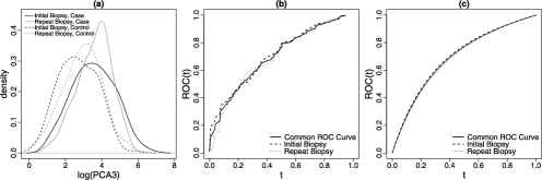
Figure 1: (a) density of $\operatorname{log}(\mathrm{PCA3})$ conditional on disease status in each population; (b) nonparametric and (c) semiparametric ROC curves for PCA3 in initial and repeat biopsy populations, and the common ROC curve adjusting for population effect.

Figure 1(a) shows probability density functions for $\operatorname{log}(\mathrm{PCA3})$ conditional on disease status, and Figure 1(b) shows the empirical ROC curves in the two populations. Interestingly, although the distributions of PCA3 conditional on disease status seem to differ between the two populations, the two ROC curves appear similar to each other. A test for equality of the ROC curves based on the area under the ROC curves yields a $p$-value of 0.66. An alternative test comparing case placement values using the Wilcoxon Rank Sum statistic yields a $p$-value of 0.45 [Huang and Pepe (2009a)]. Also presented in Figure 1(b) is the nonparametric estimate of the common ROC curve [Janes and Pepe (2009)] $\widehat{{\mathcal{A}}\operatorname{ROC}}(t)=\sum_{i=1}^{n_{D}}I\{Y_{Di}>\hat{S}_{\bar{D}X_{i}}^{-1}(t)\}/n_{D}$.

= Initial biopsy Repeat biopsy Combined-data Population specific Combined-data Population specific $\operatorname{ROC}(t)$ $t=0.1$ Est 0.266 (0.209, 0.339) 0.274 (0.205, 0.368) 0.266 (0.209, 0.339) 0.256 (0.166, 0.369) Eff^⋆ 1.57 1.00 2.53 1.00 $t=0.3$ Est 0.591 (0.518, 0.671) 0.600 (0.510, 0.704) 0.591 (0.518, 0.671) 0.578 (0.462, 0.697) Eff 1.57 1.00 2.41 1.00 $t=0.5$ Est 0.772 (0.710, 0.831) 0.778 (0.703, 0.854) 0.772 (0.710, 0.831) 0.764 (0.670, 0.847) Eff 1.64 1.00 2.21 1.00 $t=0.7$ Est 0.886 (0.836, 0.927) 0.889 (0.827, 0.939) 0.886 (0.836, 0.927) 0.882 (0.810, 0.940) Eff 1.67 1.00 2.19 1.00 $t=0.9$ Est 0.967 (0.943, 0.982) 0.967 (0.937, 0.986) 0.967 (0.943, 0.982) 0.966 (0.930, 0.987) Eff 1.67 1.00 2.32 1.00 $\operatorname{CDF}_{R}(p)$ $p=0.65$ $p=0.20$ Est 0.855 (0.711, 1.000) 0.843 (0.698, 1.000) 0.418 (0.276, 0.564) 0.406 (0.211, 0.586) Eff 1.12 1.00 1.60 1.00 $\operatorname{Risk}(y)$ $y=60$ $y=20$ Est 0.654 (0.567, 0.731) 0.659 (0.569, 0.749) 0.208 (0.147, 0.270) 0.214 (0.135, 0.292) Eff 1.22 1.00 1.59 1.00 []Eff^⋆: efficiency relative to the population-specific estimator.

Table 5: The constrained maximum likelihood estimators calculated with data from the PCA3 study

As we have noted earlier, we cannot enforce a common ROC condition by fitting a logistic model with $Y$ on the usual scale. But fitting a model with $Y$ on the $U$ scale such as $\operatorname{logit}P(D=1|U,X)=\operatorname{logit}P(D=1|X)+\beta_{0}+\beta_{1}^{T}r(U)$ automatically guarantees a common ROC across $X$. We adopt a logistic model $\operatorname{logit}P(D=1|U,X)=\operatorname{logit}P(D=1|X)+\beta_{0}+\beta_{1}U+\beta_{2}U^{2}$. Figure 1(c) displays the ROC curve estimates calculated by fitting this model separately in the two populations and by using the combined-data analysis method. Observe that the curves are all concave and are very similar to each other. However, the combined-data analysis estimates are much more precise (Table 5). Borrowing information across populations leads to an efficiency gain of over 50% compared to using the initial biopsy sample only and over 100% gain in efficiency compared to using the repeat biopsy sample only. Comparing the CML estimates of the common $\operatorname{ROC}(t)$ (combined-data analysis) with the nonparametric ${\mathcal{A}}\operatorname{ROC}(t)$ estimates [Figure 1(b)], the efficiency gains through modeling the ROC derivative are 87%, 41%, 78%, 51%, and 74%, respectively, for $t=0.1,0.3,0.5,0.7$, and $0.9$.

Figure 2: Risk as a function of $\operatorname{log}(\mathrm{PCA3})$ and versus the CDF of Risk in the (a) initial biopsy and (b) repeat biopsy populations.

The estimated risk is shown in Figure 2 as a function of $\operatorname{log}(\mathrm{PCA3})$ and the risk distributions in the two populations are shown as well. Again, curves derived from fitting the risk model to each population separately appear to be similar to those derived from the combined-data analysis. Urologists are particularly interested in the capacity of PCA3 to identify high risk subjects from the initial biopsy population and low risk subjects from the repeat biopsy population. Toward this goal, we want to have an accurate prediction of the prostate cancer risk as a function of PCA3 among each population, and to have a good assessment of the population impact of PCA3 in assisting treatment decision. Here we evaluate the risk of prostate cancer at $\mathrm{PCA}3=60$, denoted by $\operatorname{Risk}(60)$, for the former population and the risk of prostate cancer at $\mathrm{PCA}3=20$, denoted by $\operatorname{Risk}(20)$, for the latter population. In addition, suppose an estimated risk greater than 0.65 will lead to a recommendation for treatment and a risk below 0.20 will lead to a recommendation against treatment. Therefore, we assess $\operatorname{CDF}_{R}(0.65)$ in the initial biopsy population and $\operatorname{CDF}_{R}(0.20)$ in the repeat biopsy population. Table 5 presents the CML estimators for those quantities based on population-specific analysis and on combined-data analysis. Again, both approaches result in similar estimates, but combined-data analysis yields more precise estimates. The efficiency of the combined-data analysis is modest for evaluating the risk prediction capacity of PCA3 in the initial biopsy population [1.22 for estimating $\operatorname{Risk}(60)$ and 1.12 for estimating $\operatorname{CDF}_{R}(0.65)$], but much larger when the repeat biopsy population is concerned, around 1.6 for both $\operatorname{Risk}(20)$ and $\operatorname{CDF}_{R}(0.20)$. Our results provide useful information to urologists regarding the value of PCA3 in treatment decision making. In particular, based on a high risk threshold of 0.65 and a low risk threshold of 0.20, use of PCA3 will recommend 86% of subjects for treatment in initial biopsy population and will spare 58% of subjects from treatment in repeat biopsy population.

6 Discussion

In this paper we proposed a logistic regression framework for modeling marker values after they are standardized using the distribution in the nondiseased control population. This sort of standardization is often used in laboratory and clinical medicine. For example, Frischancho (1990) provides weight and height of children standardized relative to a healthy population of children of the same age and gender. Our framework provides a convenient way to connect risk modeling with ROC analysis with many applications. For example, one can use it for simply estimating the ROC curve from a single cohort or case–control study, for evaluating covariate effects on biomarker performance, and for combining data sources in evaluating biomarker performance through the estimation of a common ROC curve when applicable, as presented in this paper.

Covariate adjustment is an important issue in ROC curve evaluation. When a biomarker’s distribution depends on covariates, adjusting for the covariate effect allows an evaluation of biomarker’s classification performance independent of the covariate level. Estimation of a common ROC curve adjusting for a covariate that affects marker distribution in a classification study is analogous to estimation of a common odds ratio across covariate strata in an association study but requires different techniques for covariate adjustment. While the covariates to be adjusted for in odds ratio estimation are included in the regression model, covariate-adjustment in ROC analysis is achieved in the step of marker standardization. We developed two types of combined-data analysis estimators based on a common ROC curve. The constrained estimated maximum likelihood estimator is more efficient when there is large variability in estimated standardized marker values across populations, due, for example, to variation in the sizes of the reference nondiseased sample across populations. The estimated empirical likelihood estimator, on the other hand, is easier to implement and may be preferable for complicated models. R code for computing the two estimators is available upon request. An easy-to-implement nonparametric method for covariate-adjustment in ROC estimation has been proposed in Janes and Pepe (2008, 2009). Our logistic regression based estimator provides a much more efficient semiparametric alternative. An additional advantage of our semiparametric method over the nonparametric method is the ease of retrieving the ROC derivative, which can be used for various purposes, including the derivation of the risk distribution [Huang and Pepe (2009b)]. Moreover, while the nonparametric method does not model risk factors for risk prediction and operationally is more suitable for discrete $X$, our framework has the same flexibility as a traditional logistic regression model. Our method also provides a useful addition to the semiparmatric ROC modeling field. Unlike other existing semiparametric ROC regression methods [e.g., by Pepe and Cai (2004), Alonzo and Pepe (2002), Dodd and Pepe (2003)] that posit assumptions on the functional form of the ROC curve (typically a binormal ROC form), we fit a model to the ROC derivative directly. One attractive property of this strategy is that one can easily build in the constraint that the ROC curve is concave, which is a fundamental attribute of proper ROC curves, whereas the traditional binormal ROC model is not natural for ensuring concavity. Another attractive feature of the logistic regression framework is that it accommodates case–control sampling which is common in biomarker research studies [Pepe et al. (2001)].

Moreover, as shown in Sections 3.4 and 4, another novelty of the logistic regression framework over existing ROC regression methods based on marker standardization is the way the standardized marker values are used. Our approach fits a prospective risk model based on standardized marker values among all subjects and is more efficient compared to the traditional ROC regression methods that build on standardized marker value among cases only.

Our methods for combining data from different sources is flexible and applies whether or not the components combined have the same study design. For example, we can have one component being a case–control study and the other component a cohort study. Frequency matching in case–control studies can also be accommodated by adjusting for biased sampling in estimation of the standardized marker value and in fitting of the logistic regression model. The former can be conducted using the fact that $U(y)=P(Y>y|D=0)=\sum_{s}P(Y>y|D=0,S=s)P(D=0|S=s)$ for cases and controls frequency-matched within stratum $S$. The latter can be conducted weighting the contribution of each observation to the likelihood by the inverse of the sampling probability.

Finally, we want to point out that there are different ways to assess our model calibrations in practice. The direct correspondence between our risk model and the ROC model allows assessment of model calibration based on ROC model checking techniques such as those proposed in Cai and Zheng (2007). In our motivating example, goodness of fit can be demonstrated graphically comparing the nonparametric estimate of the covariate-adjusted ROC curve with our semiparametric estimates. Alternatively, model checking can be conducted through general Hosmer–Lemeshow type techniques developed for logistic regression [Hosmer and Lemeshow (1980), Huang and Pepe (2010b)].

References

- Alonzo and Pepe (2002) {barticle}[pbm] \bauthor\bsnmAlonzo, \bfnmTodd A.\binitsT. A. and \bauthor\bsnmPepe, \bfnmMargaret Sullivan\binitsM. S. (\byear2002). \btitleDistribution-free ROC analysis using binary regression techniques. \bjournalBiostatistics \bvolume3 \bpages421–432. \biddoi=10.1093/biostatistics/3.3.421, issn=1465-4644, pii=3/3/421, pmid=12933607 \bptokimsref \endbibitem
- Bura and Gastwirth (2001) {barticle}[mr] \bauthor\bsnmBura, \bfnmEfstathia\binitsE. and \bauthor\bsnmGastwirth, \bfnmJoseph L.\binitsJ. L. (\byear2001). \btitleThe binary regression quantile plot: Assessing the importance of predictors in binary regression visually. \bjournalBiom. J. \bvolume43 \bpages5–21. \biddoi=10.1002/1521-4036(200102)43:1<5::AID-BIMJ5>3.0.CO;2-6, issn=0323-3847, mr=1820036 \bptokimsref \endbibitem
- Cai and Zheng (2007) {barticle}[mr] \bauthor\bsnmCai, \bfnmTianxi\binitsT. and \bauthor\bsnmZheng, \bfnmYingye\binitsY. (\byear2007). \btitleModel checking for ROC regression analysis. \bjournalBiometrics \bvolume63 \bpages152–163, 312–313. \biddoi=10.1111/j.1541-0420.2006.00620.x, issn=0006-341X, mr=2345585 \bptokimsref \endbibitem
- Campbell and Ratnaparkhi (1993) {barticle}[auto:STB—2013/05/03—14:24:43] \bauthor\bsnmCampbell, \bfnmG.\binitsG. and \bauthor\bsnmRatnaparkhi, \bfnmM. V.\binitsM. V. (\byear1993). \btitleAn application of Lomax distributions in receiver operating characteristic (ROC) curve analysis. \bjournalCommunications in Statistics \bvolume22 \bpages1681–1697. \bptokimsref \endbibitem
- Deras et al. (2008) {barticle}[auto:STB—2013/05/03—14:24:43] \bauthor\bsnmDeras, \bfnmI. L.\binitsI. L., \bauthor\bsnmAubin, \bfnmS. M. J.\binitsS. M. J., \bauthor\bsnmBlase, \bfnmA.\binitsA., \bauthor\bsnmDay, \bfnmJ. R.\binitsJ. R., \bauthor\bsnmKoo, \bfnmS.\binitsS., \bauthor\bsnmPartin, \bfnmA. W.\binitsA. W., \bauthor\bsnmEllis, \bfnmW. J.\binitsW. J., \bauthor\bsnmMarks, \bfnmL. S.\binitsL. S., \bauthor\bsnmFradet, \bfnmY.\binitsY., \bauthor\bsnmRittenhouse, \bfnmH.\binitsH. and \bauthor\bsnmGroskopf, \bfnmJ.\binitsJ. (\byear2008). \btitlePCA3: A molecular urine assay for predicting prostate biopsy outcome. \bjournalJ. Urol. \bvolume179 \bpages1587–1592. \bptokimsref \endbibitem
- Dodd and Pepe (2003) {barticle}[mr] \bauthor\bsnmDodd, \bfnmLori E.\binitsL. E. and \bauthor\bsnmPepe, \bfnmMargaret Sullivan\binitsM. S. (\byear2003). \btitleSemiparametric regression for the area under the receiver operating characteristic curve. \bjournalJ. Amer. Statist. Assoc. \bvolume98 \bpages409–417. \biddoi=10.1198/016214503000198, issn=0162-1459, mr=1995717 \bptokimsref \endbibitem
- Dorfman et al. (1996) {barticle}[auto:STB—2013/05/03—14:24:43] \bauthor\bsnmDorfman, \bfnmD. D.\binitsD. D., \bauthor\bsnmBerbaum, \bfnmK. S.\binitsK. S., \bauthor\bsnmMetz, \bfnmC. E.\binitsC. E., \bauthor\bsnmLength, \bfnmR. V.\binitsR. V., \bauthor\bsnmHanley, \bfnmJ. A.\binitsJ. A. and \bauthor\bsnmDagga, \bfnmH. A.\binitsH. A. (\byear1996). \btitleProper receiver operating characteristic analysis: The bigamma model. \bjournalAcademic Radiology \bvolume4 \bpages138–149. \bptokimsref \endbibitem
- Egan (1975) {bbook}[auto:STB—2013/05/03—14:24:43] \bauthor\bsnmEgan, \bfnmJ. P.\binitsJ. P. (\byear1975). \btitleSignal Detection Theory and ROC Analysis. \bpublisherAcademic Press, \blocationNew York. \bptokimsref \endbibitem
- Frischancho (1990) {bbook}[auto:STB—2013/05/03—14:24:43] \bauthor\bsnmFrischancho, \bfnmA. R.\binitsA. R. (\byear1990). \btitleAnthropometric Standards for the Assessment of Growth and Nutritional Status. \bpublisherUniv. Michigan Press, \blocationAnn Arbor. \bptokimsref \endbibitem
- Gu and Pepe (2010) {barticle}[auto:STB—2013/05/03—14:24:43] \bauthor\bsnmGu, \bfnmW.\binitsW. and \bauthor\bsnmPepe, \bfnmM. S.\binitsM. S. (\byear2010). \btitleEstimating the diagnostic likelihood ratio of a continuous marker. \bjournalBiostatistics \bvolume12 \bpages87–101. \bptokimsref \endbibitem
- Hanley and Hajian-Tilaki (1997) {barticle}[auto:STB—2013/05/03—14:24:43] \bauthor\bsnmHanley, \bfnmJ. A.\binitsJ. A. and \bauthor\bsnmHajian-Tilaki, \bfnmK. O.\binitsK. O. (\byear1997). \btitleSampling variability of nonparametric estimate of the areas under receiver operating characteristic curves: An update. \bjournalAcademic Radiology \bvolume4 \bpages49–58. \bptokimsref \endbibitem
- Hosmer and Lemeshow (1980) {barticle}[auto:STB—2013/05/03—14:24:43] \bauthor\bsnmHosmer, \bfnmD. W.\binitsD. W. and \bauthor\bsnmLemeshow, \bfnmS.\binitsS. (\byear1980). \btitleGoodness of fit tests for the multiple logistic regression model. \bjournalComm. Statist. Theory Methods \bvolume9 \bpages1043–1069. \bptokimsref \endbibitem
- Huang (2007) {bmisc}[auto:STB—2013/05/03—14:24:43] \bauthor\bsnmHuang, \bfnmY.\binitsY. (\byear2007). \bhowpublishedEvaluating the predictiveness of continuous biomarkers. Ph.D. thesis, Univ. Washington. \bptokimsref \endbibitem
- Huang, Pepe and Feng (2007) {barticle}[mr] \bauthor\bsnmHuang, \bfnmYing\binitsY., \bauthor\bsnmPepe, \bfnmMargaret Sullivan\binitsM. S. and \bauthor\bsnmFeng, \bfnmZiding\binitsZ. (\byear2007). \btitleEvaluating the predictiveness of a continuous marker. \bjournalBiometrics \bvolume63 \bpages1181–1188, 1313. \biddoi=10.1111/j.1541-0420.2007.00814.x, issn=0006-341X, mr=2414596 \bptokimsref \endbibitem
- Huang and Pepe (2009a) {barticle}[auto:STB—2013/05/03—14:24:43] \bauthor\bsnmHuang, \bfnmY.\binitsY. and \bauthor\bsnmPepe, \bfnmM. S.\binitsM. S. (\byear2009a). \btitleBiomarker evaluation using the controls as a reference population. \bjournalBiostatistics \bvolume10 \bpages228–244. \bptokimsref \endbibitem
- Huang and Pepe (2009b) {barticle}[mr] \bauthor\bsnmHuang, \bfnmY.\binitsY. and \bauthor\bsnmPepe, \bfnmM. S.\binitsM. S. (\byear2009b). \btitleA parametric ROC model-based approach for evaluating the predictiveness of continuous markers in case-control studies. \bjournalBiometrics \bvolume65 \bpages1133–1144. \biddoi=10.1111/j.1541-0420.2009.01201.x, issn=0006-341X, mr=2756501 \bptokimsref \endbibitem
- Huang and Pepe (2009c) {barticle}[mr] \bauthor\bsnmHuang, \bfnmYing\binitsY. and \bauthor\bsnmPepe, \bfnmMargaret Sullivan\binitsM. S. (\byear2009c). \btitleSemiparametric methods for evaluating risk prediction markers in case-control studies. \bjournalBiometrika \bvolume96 \bpages991–997. \biddoi=10.1093/biomet/asp040, issn=0006-3444, mr=2767284 \bptokimsref \endbibitem
- Huang and Pepe (2010a) {barticle}[mr] \bauthor\bsnmHuang, \bfnmY.\binitsY. and \bauthor\bsnmPepe, \bfnmM. S.\binitsM. S. (\byear2010a). \btitleSemiparametric methods for evaluating the covariate-specific predictiveness of continuous markers in matched case-control studies. \bjournalJ. R. Stat. Soc. Ser. C. Appl. Stat. \bvolume59 \bpages437–456. \biddoi=10.1111/j.1467-9876.2009.00707.x, issn=0035-9254, mr=2756544 \bptokimsref \endbibitem
- Huang and Pepe (2010b) {barticle}[mr] \bauthor\bsnmHuang, \bfnmYing\binitsY. and \bauthor\bsnmPepe, \bfnmMargaret Sullivan\binitsM. S. (\byear2010b). \btitleAssessing risk prediction models in case-control studies using semiparametric and nonparametric methods. \bjournalStat. Med. \bvolume29 \bpages1391–1410. \biddoi=10.1002/sim.3876, issn=0277-6715, mr=2758124 \bptokimsref \endbibitem
- Huang, Pepe and Feng (2013) {bmisc}[auto:STB—2013/05/03—14:24:43] \bauthor\bsnmHuang, \bfnmY.\binitsY., \bauthor\bsnmPepe, \bfnmM. S.\binitsM. S. and \bauthor\bsnmFeng, \bfnmZ.\binitsZ. (\byear2013). \bhowpublishedSupplement to “Logistic regression analysis with standardized markers.” DOI:\doiurl10.1214/13-AOAS634SUPP. \bptokimsref \endbibitem
- Janes and Pepe (2008) {barticle}[mr] \bauthor\bsnmJanes, \bfnmHolly\binitsH. and \bauthor\bsnmPepe, \bfnmMargaret S.\binitsM. S. (\byear2008). \btitleAdjusting for covariates in studies of diagnostic, screening, or prognostic markers: An old concept in a new setting. \bjournalAm. J. Epidemiol. \bvolume168 \bpages89–97. \bptokimsref \endbibitem
- Janes and Pepe (2009) {barticle}[mr] \bauthor\bsnmJanes, \bfnmHolly\binitsH. and \bauthor\bsnmPepe, \bfnmMargaret S.\binitsM. S. (\byear2009). \btitleAdjusting for covariate effects on classification accuracy using the covariate-adjusted receiver operating characteristic curve. \bjournalBiometrika \bvolume96 \bpages371–382. \biddoi=10.1093/biomet/asp002, issn=0006-3444, mr=2507149 \bptokimsref \endbibitem
- Metz and Pan (1999) {barticle}[mr] \bauthor\bsnmMetz, \bfnmCharles E.\binitsC. E. and \bauthor\bsnmPan, \bfnmXiaochuan\binitsX. (\byear1999). \btitle“Proper” binormal ROC curves: Theory and maximum-likelihood estimation. \bjournalJ. Math. Psych. \bvolume43 \bpages1–33. \biddoi=10.1006/jmps.1998.1218, issn=0022-2496, mr=1669506 \bptokimsref \endbibitem
- Pepe (2003) {bbook}[mr] \bauthor\bsnmPepe, \bfnmMargaret Sullivan\binitsM. S. (\byear2003). \btitleThe Statistical Evaluation of Medical Tests for Classification and Prediction. \bseriesOxford Statistical Science Series \bvolume28. \bpublisherOxford Univ. Press, \blocationOxford. \bidmr=2260483 \bptokimsref \endbibitem
- Pepe and Cai (2004) {barticle}[mr] \bauthor\bsnmPepe, \bfnmMargaret Sullivan\binitsM. S. and \bauthor\bsnmCai, \bfnmTianxi\binitsT. (\byear2004). \btitleThe analysis of placement values for evaluating discriminatory measures. \bjournalBiometrics \bvolume60 \bpages528–535. \biddoi=10.1111/j.0006-341X.2004.00200.x, issn=0006-341X, mr=2067011 \bptokimsref \endbibitem
- Pepe et al. (2001) {barticle}[pbm] \bauthor\bsnmPepe, \bfnmM. S.\binitsM. S., \bauthor\bsnmEtzioni, \bfnmR.\binitsR., \bauthor\bsnmFeng, \bfnmZ.\binitsZ., \bauthor\bsnmPotter, \bfnmJ. D.\binitsJ. D., \bauthor\bsnmThompson, \bfnmM. L.\binitsM. L., \bauthor\bsnmThornquist, \bfnmM.\binitsM., \bauthor\bsnmWinget, \bfnmM.\binitsM. and \bauthor\bsnmYasui, \bfnmY.\binitsY. (\byear2001). \btitlePhases of biomarker development for early detection of cancer. \bjournalJ. Natl. Cancer Inst. \bvolume93 \bpages1054–1061. \bidissn=0027-8874, pmid=11459866 \bptokimsref \endbibitem
- Pepe et al. (2008) {barticle}[auto:STB—2013/05/03—14:24:43] \bauthor\bsnmPepe, \bfnmM. S.\binitsM. S., \bauthor\bsnmFeng, \bfnmZ.\binitsZ., \bauthor\bsnmHuang, \bfnmY.\binitsY., \bauthor\bsnmLongton, \bfnmG. M.\binitsG. M., \bauthor\bsnmPrentice, \bfnmR.\binitsR., \bauthor\bsnmThompson, \bfnmI. M.\binitsI. M. and \bauthor\bsnmZheng, \bfnmY.\binitsY. (\byear2008). \btitleIntegrating the predictiveness of a marker with its performance as a classifier. \bjournalAmerican Journal of Epidemiology \bvolume167 \bpages362–368. \bptokimsref \endbibitem
- Qin and Lawless (1994) {barticle}[mr] \bauthor\bsnmQin, \bfnmJing\binitsJ. and \bauthor\bsnmLawless, \bfnmJerry\binitsJ. (\byear1994). \btitleEmpirical likelihood and general estimating equations. \bjournalAnn. Statist. \bvolume22 \bpages300–325. \biddoi=10.1214/aos/1176325370, issn=0090-5364, mr=1272085 \bptokimsref \endbibitem
- Qin and Zhang (1997) {barticle}[mr] \bauthor\bsnmQin, \bfnmJing\binitsJ. and \bauthor\bsnmZhang, \bfnmBiao\binitsB. (\byear1997). \btitleA goodness-of-fit test for logistic regression models based on case-control data. \bjournalBiometrika \bvolume84 \bpages609–618. \biddoi=10.1093/biomet/84.3.609, issn=0006-3444, mr=1603924 \bptokimsref \endbibitem
- Qin and Zhang (2003) {barticle}[mr] \bauthor\bsnmQin, \bfnmJing\binitsJ. and \bauthor\bsnmZhang, \bfnmBiao\binitsB. (\byear2003). \btitleUsing logistic regression procedures for estimating receiver operating characteristic curves. \bjournalBiometrika \bvolume90 \bpages585–596. \biddoi=10.1093/biomet/90.3.585, issn=0006-3444, mr=2006837 \bptokimsref \endbibitem