Influencing elections with statistics: Targeting voters with logistic regression trees

Abstract

In political campaigning substantial resources are spent on voter mobilization, that is, on identifying and influencing as many people as possible to vote. Campaigns use statistical tools for deciding whom to target (“microtargeting”). In this paper we describe a nonpartisan campaign that aims at increasing overall turnout using the example of the 2004 US presidential election. Based on a real data set of 19,634 eligible voters from Ohio, we introduce a modern statistical framework well suited for carrying out the main tasks of voter targeting in a single sweep: predicting an individual’s turnout (or support) likelihood for a particular cause, party or candidate as well as data-driven voter segmentation. Our framework, which we refer to as LORET (for LOgistic REgression Trees), contains standard methods such as logistic regression and classification trees as special cases and allows for a synthesis of both techniques. For our case study, we explore various LORET models with different regressors in the logistic model components and different partitioning variables in the tree components; we analyze them in terms of their predictive accuracy and compare the effect of using the full set of available variables against using only a limited amount of information. We find that augmenting a standard set of variables (such as age and voting history) with additional predictor variables (such as the household composition in terms of party affiliation) clearly improves predictive accuracy. We also find that LORET models based on tree induction beat the unpartitioned models. Furthermore, we illustrate how voter segmentation arises from our framework and discuss the resulting profiles from a targeting point of view.

abstract skip 20 keyword skip 8 frontmatter skip 0plus 3minus 3

, , , and

1 Introduction.

“Decisions are made by those who show up,” said President Bartlet, a character from a popular TV show, The West Wing. The character in the show used the line to motivate a college audience to voice their opinion by showing up at the polls. Getting eligible voters to actually vote (“get-out-the-vote;” GOTV) is an important goal in countries with a democratic political system and a lot of resources are spent on achieving that goal. Take the 2012 US presidential race, for example. In that year, the world witnessed the amount of money raised and spent by the campaigns reaching unprecedented heights. By spending over USD $1.5$ billion, the Obama and Romney campaigns tried to mobilize eligible voters to engage in the political process and cast their vote on November 6th.

1.1 Campaigning, mobilization and turnout.

The impact of partisan campaigning or nonpartisan get-out-the-vote efforts on mobilization and turnout has been subject to numerous scientific investigations over the last 20 years. Examples include Whitelock, Whitelock and van Heerde’s (2010) survey on the effect of campaigning and turnout in the UK and Germany or Karp and Banducci (2007) who surveyed the relationship between party contacts and turnout in 23 countries (old and new democracies). See also Holbrook and McClurg (2005) for an overview of recent studies. Starting from an early “minimal effect” hypothesis [Finkel (1993), i.e., the idea that political campaigns barely influence turnout], there is evidence in the literature that campaigning does indeed have a measurable effect on persuasion or mobilization of the electorate [Holbrook and McClurg (2005)], which is supported by a number of experimental studies, for example, Nickerson, Friedrichs and King (2006), Gerber and Green (2000a, 2000b), Green, Gerber and Nickerson (2003), Phillips, Urbany and Reynolds (2008), Hansen and Bowers (2009), Arceneaux and Nickerson (2009).

Reinforced by these results, campaigns are spending large amounts of money on mobilizing voters. However, one cannot simply equate higher spending with higher turnout. Take the United States, for example, where the “professionalization” [Muller (1999)] of campaigning had its origin [Plasser (2000)] and spread to many democratic countries all over the world [Sussman and Galizio (2003)]. Arguably, nowhere else is political campaigning a bigger business then in the US and nowhere else is more money being spent on convincing people to cast their ballots. Despite increased political consultancy, monumental campaign efforts and large out-laying of resources, the average voter turnout since 1980 during the Presidential election years has only been $56\%$; see also Table 1. This raises questions about the effectiveness of campaigns’ voter mobilization strategies.

Table 1: Individual and aggregated turnout rate (votes for highest office divided by the voting-eligible population) for presidential elections in the United States and the money spent by all candidates (in million USD). The fourth column lists the real expenditures (inflation-adjusted at 2008 rates). Sources: McDonald (2012) and http://www.opensecrets.org/, accessed 11-21-2012 (all elections until 2008), Wikipedia (2012) and The New York Times (http://elections.nytimes.com/2012/campaign-finance, accessed 11-21-2012) (2012 election). Inflation-adjustment has been done with http://www.bls.gov/data/inflation_calculator.htm at 11-21-2012

		Expenditures	Real expenditures
Year	Turnout (in %)	(in mill. USD)	(at 2008 rates)
2012	$57.5$	$1605.2$	$1494.7$
2008	$61.7$	$1324.7$	$1324.7$
2004	$60.1$	$717.9$	$818.2$
2000	$54.2$	$343.1$	$429.0$
1996	$51.7$	$239.9$	$329.2$
1992	$58.1$	$192.2$	$295.0$
1988	$52.8$	$210.7$	$383.5$
1984	$55.2$	$103.6$	$214.7$
1980	$54.2$	$92.3$	$241.2$
Mean	$56.2$	$536.6$	$614.5$
Sd	$3.4$	$562.5$	$486.2$
Min	$51.7$	$92.3$	$214.7$
Max	$61.7$	$1605.7$	$1494.7$

Figure 1: The usual partisan campaign classification of targeting groups.

1.2 How is targeting carried out?

Voter mobilization is a two-step process [cf. Goldstein and Ridout (2002)]. In the first step, campaigns need to identify people suitable to direct their mobilization efforts at (also known as voter targeting). The second step involves crafting measures that best motivate these people to turn up at the polls, that is, to assure the effectiveness of mobilization. The latter step includes decisions on which tactics best translate to mobilization and has been investigated by researchers in the political and social sciences or marketing [for an overview of which measures to use see, e.g., Green and Gerber (2008)]. The first step (identifying the “right” recipients for mobilization messages) has, to the best of our knowledge, been addressed rather infrequently in the scientific literature. Notable exceptions are Wielhouwer (2003), Parry et al. (2008), Murray and Scime (2010) or Imai and Strauss (2011).

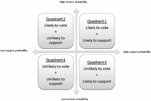
When identifying people to target, campaigns typically first assess two important aspects for each eligible voter: (a) likelihood of support (for a particular cause, party or candidate) and (b) likelihood to turnout at the polls [Malchow (2008), Issenberg (2012b)]. Using these two assessments, each voter can be schematically classified into one of four possible categories (or “quadrants,” see Figure 1). For voters that are classified into quadrant 1 (likely to vote and likely to support), campaigns usually allocate few resources on mobilization (but these voters might be asked to help out with the campaign). Eligible voters assigned to quadrant 2 (likely to vote but unlikely to support) are “targeted for support” by the campaigns, as they can be persuaded to become supporters. In quadrant 3 (unlikely to vote but likely to support), the focus of the targeting effort will be on mobilization for turnout (“targeting for turnout”). For both quadrants 2 and 3 the campaigns will use targeted messages. The messages could be customized to individuals based on their demographic and behavioral data (“voter profiles”). Voters classified to belong to quadrant 4 (unlikely to vote and unlikely to support) will typically not be targeted by a campaign [see also Issenberg (2012b)].

In order to populate quadrants 1–4, campaigns need rich voter data and powerful data models that can predict, for each individual person, his/her probability of support or turnout with as high accuracy as possible. In some countries, voting data that can be used to explain and predict voting behavior is available as public data. In the US, for example, states collect and report voter registration information and make them publicly available. Collection is done at the county level and the data are only available in aggregated fashion. Individual voting data is usually not readily and easily accessible [US Election Assistance Commission (2010)]. Data for targeting also arrives in the form of proprietary information, offered by data vendors who supply individual-level data and add considerable details about voter behavior and demographics. In many countries, proprietary sources from market research companies are the only way to obtain data for targeting, as public data are scarce.

For all data sources the most important predictor variables typically collected are records of the (individual) voting history. The ability of voting history as a predictor for future election attendance has long been recognized [e.g., Denny and Doyle (2009)] and, consequently, for targeting purposes voting history is heavily relied on [Goldstein and Ridout (2002), Malchow (2008)]. Additional predictive power has been found in sociodemographic or personality variables like age, income and party affiliation.

While campaigns can collect an abundance of predictor variables with ease, collecting information on the target variable poses a more challenging problem. Supervised classification methods require a known target (i.e., observations on the response variable) in order to train the model. In the case of an election, the target (i.e., whether a person will truly turnout or support) is not known until the election is over. Campaigns therefore have to rely on suitable proxy target variables which should most accurately resemble the true outcome. The usage of proxies renders the application of supervised classification procedures during or before the election feasible. While many proxies (e.g., an earlier election) are imaginable and the choice may vary between campaigns, proxy variables often arrive in the form of carefully designed polls about voting intention. For example, the Obama 2012 campaign conducted short, parallel survey polls on random samples of 8000 to 9000 voters from “battleground states” every night during the final phase of the campaign [Blumenthal (2012)]. For the rest of this paper we only consider the situation of either employing the true outcome or proxy variables derived from surveys, but we have also investigated the use of proxy variables derived from previous election outcomes; see the supplementary material [Rusch et al. (2013b)].

Campaigns often have access to similar sources of information, but the way the information is processed, modeled and ultimately acted on can be very diverse. Traditionally, campaigns have relied on simple deterministic rules for choosing whom to target by, for example, using information from the last four comparable elections as the main predictors for future voting behavior. Intuitively, someone who voted in all four out of the last four elections is seen as a likely voter, whereas someone who did not vote in any of the four elections is considered unlikely to vote in the upcoming election. However, predicting the behavior of a person with a mixed voting pattern (i.e., voted in the last election but not in the previous three) by simple deterministic rules is ambiguous and can be suboptimal, as the procedure lacks the ability to learn structure from a data set.

This has sparked interest in adopting probabilistic approaches in place of deterministic rules based solely on the voting history [Issenberg (2012b)]. For instance, Malchow (2008) promotes a linear probability model as well as tree-like models such as CHAID [Kass (1980)] for political microtargeting. Murray and Scime (2010) suggest decision trees as well. Green and Kern (2012) advocate Bayesian additive trees [BART, Chipman, George and McCulloch (2010)] and Imai and Strauss (2011) propose to use classification trees, which they embed in a decision theoretic framework for optimal planning of GOTV campaigns. Other state-of-the-art approaches that are used include logistic or probit regression.

1.2.1 Targeting for turnout.

In the specific case of using probabilistic models for targeting for turnout, the two tasks of identifying likely voters and likely supporters from Figure 1 coincide. Here, campaigns are interested in assigning each voter an individual probability to show up at election day. Based on these estimated probabilities, Malchow (2008) reasons that using targeting plans on people with values around $0.5$ is worthwhile, whereas targeting people with predicted probabilities near $0$ or $1$ is considered a waste. Given a high accuracy of the predictions, a person with a predicted probability close to zero is unlikely to vote, regardless of how compelling the mobilization message is. A person with a predicted probability of 1 is going to turn out at the polls anyways, even without the need for extra persuasion. In both cases, targeting those people would not lead to an increase in turnout, yet it would consume resources and hence be wasteful. However, voters with a predicted probability in a “targeting range” around $0.5$ may be “convincable” to show up at the polls using the right incentive. Malchow (2008) suggests a targeting range of $[0.3,0.7]$. Clearly, we can be hopeful to sway a person with a probability of voting of, say, $0.35$, as long as we get the right message to her. Also, while a person with a probability of, say, $0.68$ might be going to vote without being targeted specifically, it should not hurt to encourage her a bit more.

2 A new unified statistical framework for voter targeting.

In this paper we introduce a flexible statistical framework for the task of voter microtargeting and apply it to a (virtual) nonpartisan GOTV campaign that uses different sets of predictor variables. The main contribution of this framework is that it allows prediction and segmentation in a single step. It generalizes two standard models currently used in political targeting: it encompasses logistic regression as well as classification trees and also allows for a combination of both within the same model. We refer to the resulting framework as LOgistic REgression Tree (LORET) models. LORET models are very flexible in that, in their simplest form, they reduce to a majority vote model; they also allow regression-like modeling with predictors (with small adjustment it works for all generalized models for binary data such as probit models) as well as hierarchical partitioning of the feature space under the same umbrella.

Based on a novel data set of Ohio voters which is prototypical for what campaigns can buy from data providers, we investigate LORET models of varying degrees of flexibility and compare them with a particular focus on the benefits they provide for targeting voters. While we illustrate LORET models for assessing the probability of turnout only, we are quick to point out that LORET models can also be used to gauge a voter’s probability of supporting a candidate or cause. We show that LORET models can have higher predictive accuracy than logistic regression alone, may lead to better interpretability compared to classification trees, allow for automatic data-driven creation of voter profiles, conduct variable selection and allow for inclusion of substantive knowledge and experience via the logistic model.

This paper is organized as follows. In Section 3 we present a statistical framework for voter targeting that combines logistic regression models with recursive partitioning. Section 4 describes the case study of applying the methods to a (virtual) nonpartisan GOTV campaign in Ohio that set increasing overall turnout in the US presidential general election in 2004 as its goal. We illustrate using the LORET framework in a situation where we have labeled training data for a sample of eligible voters (Section 4.4). In Section 4.5 we discuss the creation of model-based voter profiles for targeting and illustrate how they arise naturally within the LORET framework. We finish with conclusions and some general remarks on the usage of LORET in Section 5. This paper is accompanied by supplementary material [Rusch et al. (2013a)].

3 LORET: Modeling and predicting voting behavior.

Logistic regression and tree-based methods are popular methods for turnout prediction and voter targeting [Malchow (2008)]. Using this as a backdrop, we introduce a general framework—logistic regression trees (LORET)—that encompasses and extends these methods. Briefly, the idea is the following: Instead of fitting a global logistic regression model to the whole data, one might fit a collection of local regression models to subsets or segments of the data (i.e., a segmented logistic regression model) in order to obtain a better fit and higher predictive accuracy. Since usually the “correct” segmentation is not known, it needs to be learned from the data, for example, by using recursive partitioning methods.

In what follows we start with the general formulation of logistic regression models for one or more segments and then show how for more than one segment the segmentation can be estimated with recursive partitioning.

3.1 Segmented logistic regression.

Let $y_{i}\in\{0,1\}$ denote a Bernoulli random variable for the $i$th observation, $i=1,\ldots,N$, and $\mathbf{x}_{i}$ denote a $(p+1)$-dimensional vector of $p$ covariates and one intercept, $(1,x_{i1},\ldots,x_{ip})^{\top}$. Let us assume there are $r$ (known or estimated) disjoint segments in the data. For each segment $k=1,\ldots,r$, we can then specify a logistic regression model for the relationship between $y$ and $x_{1},\ldots,x_{p}$ within that segment,

$$P\bigl{(}y_{i}=1|x_{i1},\ldots,x_{ip};\bolds{\beta}^{(k)}\bigr{)}=\pi_{i}=\frac{\exp(\mathbf{x}_{i}^{\top}\bolds{\beta}^{(k)})}{1+\exp(\mathbf{x}_{i}^{\top}\bolds{\beta}^{(k)})},$$ (1)

where $k=k(i)$ is the segment to which observation $i$ belongs and $\pi_{i}$ denotes the probability to belong to class “1” (e.g., “vote${}={}$yes”). The segment-specific parameter vector is $\bolds{\beta}^{(k)}$ and its estimates are referred to as $\hat{\bolds{\beta}}^{(k)}$, which can be easily obtained (given the segmentation) via maximum likelihood [see, e.g., McCullagh and Nelder (1989)]. Based on the associated predicted probabilities, classification can then be done by

$$\hat{y}_{i}(c_{0})=\cases{1,&\quad$\mbox{if }\hat{\pi}_{i}\geq c_{0},$\vspace*{2pt}\cr 0,&\quad$\mbox{if }\hat{\pi}_{i}<c_{0},$}$$ (2)

where $c_{0}\in[0,1]$ is a specific cutoff value (but could, in principle, also be specified to be different for different segments).

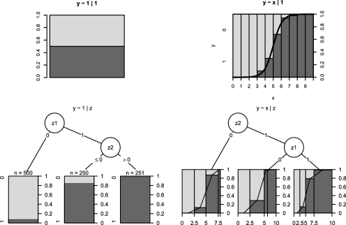
If there is only a single segment (i.e., a root node and hence a known segmentation), LORET in (1) reduces to a standard logistic regression model. Here the parameters of the linear decomposition of the conditional mean of the logit-transformed response variable $y$ are estimated given the status of $p$ covariates. Evaluation of the logistic model at the estimated parameter vector $\hat{\bolds{\beta}}$ yields the predicted probabilities, $\hat{\pi}_{i}$. If the model uses no covariates as regressors, it further reduces to a majority vote model, that is, a logistic regression model with only an intercept or simply the relative frequency of class “1” transformed to the logit scale. The upper row in Figure 2 illustrates majority vote and logistic regression on an artificial set of data with a single continuous covariate $x$. The former fits a single constant (the prevalence of “1”), the latter a single logistic function of $x$ to the entire data set.

Figure 2: A visualization of the different cases of LORET. In the upper left panel there is the $y\sim 1|1$ LORET, fitting a constant. In the upper right the $y\sim x|1$ LORET (logistic regression) is displayed, which is a single function of $x$ for the whole data set. The lower left panel displays a $y\sim 1|z$ LORET where the data set is partitioned based on the state of predictor variables $z$ and in each partition a constant is fitted. In the lower right panel, the $y\sim x|z$ LORET can be found. Here the data set is again partitioned based on $z$, but this time a logistic function of $x$ is fitted in the partitions. Hence, it combines the $y\sim 1|z$ and $y\sim x|1$ LORET.

If there were more than one segment and the segmentation were known, then LORET can still be simply seen as estimating a maximum likelihood model from a binomial likelihood in each segment. To estimate it, one needs to specify a logistic regression model with additional main effects for the categorical covariates (factors) corresponding to the segments and the interactions between the segment-factors and the predictors, but this still falls into the standard theory of generalized linear models [McCullagh and Nelder (1989)].

If the segmentation is unknown, however, it needs to be learned from the data. Two popular approaches for achieving this are using mixture models (e.g., mixtures of experts or latent class regression) or employing some type of algorithmic search method. Recursive partitioning is a popular example of the latter [with the result often called a “tree”, Zhang and Singer (2010)]. Trees are usually induced by splitting the data set along a function of the predictor variables into a number of partitions or segments. The segments are usually chosen by minimizing an objective function (e.g., a heterogeneity measure or a negative log-likelihood) for each segment. The procedure is then repeated recursively for each resulting partition. This approach approximates real segments in the data and yields a segmentation for which maximum likelihood estimation of parameters in each segment can be carried out, as is done in LORET.

3.2 Recursive partitioning.

Let us assume we have an additional, $\ell$-dimensional covariate vector $\mathbf{z}=(z_{1},\ldots,z_{\ell})$. Based on these covariates, we learn the segmentation, that is, we search for $r$ disjoint cells that partition the predictor subspace. Depending on whether the logistic model used for $y$ in each segment has any covariates or just a constant as regressors, there are two algorithmic approaches we can use: classification trees and trees with logistic node models.

3.2.1 Classification trees.

If the logistic model is an intercept-only model and we have a number of partitioning variables $z_{1},\ldots,z_{\ell}$, then LORET can be estimated as a classification tree. An illustration of a classification tree can be found in the lower left panel of Figure 2, where the data is first partitioned into three subsets and an intercept-only model is fitted to each subset separately. Hence, in each terminal node the model is a constant. A wide variety of algorithms have been developed to fit classification trees, among them are CHAID [Kass (1980)], CART [Breiman et al. (1984)], C4.5 [Quinlan (1993)], QUEST [Loh and Shih (1997)], CTree [Hothorn, Hornik and Zeileis (2006)] and many others. In this paper, we use CART and CTree which, respectively, are examples of tree algorithms that are biased or unbiased in variable selection.

3.2.2 Trees with logistic node models.

If there are partitioning variables $\mathbf{z}=(z_{1},\ldots,z_{\ell})$ as well as regressor variables $\mathbf{x}=(1,x_{1},\ldots,x_{p})$ for the logistic node model, we get the most general type of LORET, which is a “model tree.” The situation is illustrated in the lower right panel in Figure 2. Like in a classification tree, the data is first partitioned into subsets. However, in contrast to a classification tree, separate logistic regressions with regressors are employed in each terminal node. Thus, the resulting model tree essentially combines data-driven partitioning as done by classification trees with model-based prediction in a single approach. Different algorithms have been proposed to estimate model trees with logistic node models, including the following: SUPPORT [Chaudhuri et al. (1995)], LOTUS [Chan and Loh (2004)], LMT [Landwehr, Hall and Eibe (2005)] and MOB [Zeileis, Hothorn and Hornik (2008)]. In what follows, we will use the MOB algorithm with a logistic node model for estimating the most general version of LORET, as it proved to have good properties [Rusch and Zeileis (2013)].

Table 2: Various instances of LORET

Method	Regressor variables	Partitioning variables	Schema
Majority vote	none	none	$y\sim 1|1$
Logistic regression	yes	none	$y\sim x|1$
Classification tree	none	yes	$y\sim 1|z$
Model tree	yes	yes	$y\sim x|z$

To simplify notation and to stress the similarities, we will use a simple schema to refer to the different LORET types (cf. Table 2 and Figure 2): Majority vote models will be referred to as $y\sim 1|1$, global logistic regression models as $y\sim x|1$, classification tree models as $y\sim 1|z$ and full LORET model as $y\sim x|z$.

The LORET framework can be employed for various tasks during a voter targeting or get-out-the-vote campaign. To illustrate the usage of LORET in a campaign’s voter targeting strategy, we use a unique, proprietary data set from the 2004 general presidential election in Ohio, USA.

4 Case study: Get-out-the-vote in Ohio.

We apply our methodology to a (fictional) nonpartisan get-out-the vote campaign in Ohio, USA, whose goal it is to increase voter turnout. We choose Ohio because it has proven to be a pivotal state in about every US presidential election since 1964. Also, in every US presidential election since 2000, the difference between the Republican and Democratic candidates has been equal or less than 4%, making it a top battleground state in every recent election. The campaign we describe pertains to the 2004 US presidential election.

Our data set originates from a data vendor who adds value to public records by collecting, maintaining, updating and expanding upon public data. In the US, vendor voter data typically includes the name, address, phone, gender, party affiliation, age, vote history (elections that each voter voted) or ethnicity. US data vendors standardize the data by each state or county and by adding other potentially relevant behavioral information such as income, type of occupation, education, presence of children, property status (rental or owning) and charities that the person donated to.

4.1 Data description.

For illustration we use a proprietary data set which was provided by one of the leading nonpartisan data vendors in the industry. The data set consists of records from $19\mbox{,}634$ eligible and registered voters from Ohio. It includes a total of $77$ variables, many of which are sociodemographic categorical variables like gender, job category or education level. The data set also contains records on past voting behavior from 1990 to 2004 in general elections, primary or presidential primary elections and other elections, all coded as binary variables—that is, voted (“yes”) or not (“no”). We added three composite or aggregate variables: the raw count of elections a person attended, the number of elections a person attended since registering and the relative frequency of attended elections since registering. After removal of missing values and inconsistent entries (366 cases) there are a total of $N=19\mbox{,}634$ records with $80$ variables per record. The variable we want to predict is the individual turnout likelihood in the 2004 US presidential election.

4.2 Two sets of predictors: Voting history only vs. kitchen sink data.

The data available to campaigns can vary vastly. Some campaigns have a huge number of variables on millions of eligible voters available, as was the case with President Obama’s re-election campaign in 2012 [Project “Narwhal”, Issenberg (2012a)]. Smaller campaigns may have more limited information available. For all cases, however, the literature on voter targeting suggests that the most commonly used piece of information is the person’s voting history [Malchow (2008)], although often taking into account a person’s age [Malchow (2008), Karp, Banducci and Bowler (2008)] is recommended. One of the goals of this case study is to investigate whether including additional information (besides a person’s voting history and age) into the targeting model is beneficial. To that end, we compare and contrast two sets of predictors:

• The first set employs the standard information used by many campaigns, which is also recommended in the literature. These standard variables are a person’s voting history, recorded over the last four elections, and age. We call this set “$s$” for “standard.”

• The second set contains all other variables available, that is, the “kitchen sink.” In our case this includes variables like gender, occupation, living situation, party affiliation, party makeup of the household (“partyMix”), position within the family (“hhRank” and “hhHead”), donations for various causes, education level, relative frequency of attended elections so far (“attendance”) and many others. These variables constitute a set of additional variables, labeled “$e$” for “extended.”

4.3 Model specification for the Ohio voters.

The combination of the two variable sets with the different LORET models leads to model specifications as displayed in Table 3. The models either employ only the standard set of variables or the combination of the standard and the extended set. For unpartitioned models, the parameters are estimated with maximum likelihood. If a partition is induced, we learn it with three different algorithms (CART, CTree and MOB), depending on the nature of the node model. Please note that if age is specified as a parameter in the logistic model part (i.e., for models $y\sim s|1$, $y\sim s+e|1$ and $y\sim s|e$), a quadratic effect will be used [based on goodness-of-fit considerations; see also Parry et al. (2008)].

Table 3: LORET versions combined with the two variable groups and the algorithms used to estimate the partition. The standard variable set of age and voting history is labeled “$s$” and the set of additional variables with “$e$” (hence all variables together are “$s+e$”)

LORET	Regressor variables	Partitioning variables	Partitioning algorithm
$y\sim 1|1$	none	none	–
$y\sim s|1$	$s$	none	–
$y\sim s+e|1$	$s+e$	none	–
$y\sim 1|s$	none	$s$	CART, CTree
$y\sim 1|s+e$	none	$s+e$	CART, CTree
$y\sim s|e$	$s$	$e$	MOB

All recursive partitioning algorithms that we employ allow for tuning with metaparameters. These tuning parameters can be used to avoid overfitting of the tree algorithms and control how branchy the tree becomes. Quite generally, it can be said that the less branchy a tree is, the less prone it is to overfitting. In the algorithms we can use a higher number of observations per node, a lower tree depth and a stricter split variable selection criterion that all lead to smaller trees. At the same time the specification of metaparameters should grant enough flexibility for the algorithm to approximate a complex nonlinear relationship in the data.

For CART the maximal depth of the tree and the minimum number of observation per node (minsplit) are available to control the tree appearance. We use a maximal tree depth of $7$ and a minsplit of $100$ (which corresponds to roughly $0.5\%$ of the observations). For CTree and MOB the significance level of the association or stability tests, respectively, and the minimum number of observation per node can be used to tune the algorithm and pre-prune the trees. We employ a global significance level of $\alpha=1\times 10^{-6}$. This is sensible since the high number of observations might easily lead to significant results mainly due to the sample size. Hence, we reduce the chance of “false positive” selection of a split variable or split point by specifying a low significance level. This also functions as “automatic regularization,” as the test statistics used to decide whether to split a node have to become larger the larger the tree becomes. For minsplit we use $100$ for CTree (the same as for CART) and $1000$ for MOB which enables reliable estimation of the node model. Please note that the results were not sensitive to the choice of metaparameters. For CART, we explored depths from $3$ to $20$. For the global significance levels of CTree and MOB, we explored values of $0.0001$, $0.0005$, $0.001$, $0.005$, $0.01$, $0.05$ and $0.1$. For the minimum number of observations a node must contain we explored values of $20$, $50$, $100$, $150$, $200$, $250$ and $500$ for all methods. For these choices of depth, number of observations per node and significance level, the results were very similar.

In what follows we illustrate targeting based on LORET. We start with voter targeting in a setting where proxy data about the voting behavior for a sample of individuals in the upcoming election is available (e.g., from a poll). We then highlight the use of LORET for the creation of voter profiles.

4.4 Predicting individual turnout.

Typically the individual turnout is only known after the election is over. This makes the application of supervised procedures like LORET during or before the election challenging, since supervised procedures rely on a labeled training set in order to derive predictions. It is therefore imperative for campaigns to obtain labeled proxy data prior to closing of the election booths that most accurately resembles the true outcome. These data will often arrive from carefully designed, reliable, repeated polls about voting intention. Information gathered this way can be turned into labels for training a supervised classification model. For our virtual campaign to mobilize Ohio voters, we simulate this by estimating LORET via a training set drawn randomly (see also further below) from the entire data. Other proxies that can be used are past election results. (We also investigated our method with using the previous presidential election as proxy variable. The predictive accuracy was low—around 0.72, with majority vote having an accuracy of 0.7. We concluded that this is no viable alternative to surveys of people’s voting intentions, so we refrained from presenting the results in the main paper. The supplementary material [Rusch et al. (2013b)] contains a thorough account of that analysis.)

4.4.1 Learning and test samples via bootstrapping.

We simulate the targeting situation based on labeled training data by drawing a bootstrap sample [see, e.g., Hastie, Tibshirani and Friedman (2009)], that is, a learning set of size $N$ which is sampled randomly (with replacement) from the entire set of data and use this as our training set. To the learning set we fit a LORET model and use the model to predict the out-of-bag (oob) test set which consists of observations that were not part of the learning sample and thus basically treating them as having an unknown label. To evaluate and compare the different models, we employ the benchmarking framework of Hothorn et al. (2005). Ten folds of learning and test samples $f=1,\ldots,10$ are used. To provide a further benchmark, we also train and evaluate all models on the whole data set. This allows us to gauge the tendency of a model to overfit as well as how close out-of-bag and in-sample performance are.

4.4.2 Measuring predictive accuracy.

For each method, we assess the classification accuracy ($\mathit{acc}_{f}$) on each oob test set $f$ at a given cutoff value $c_{0}=0.5$ (for simplicity, we use the same cutoff value of $0.5$ for all segments $k$). To estimate overall predictive accuracy, we use the average over all bootstrap samples $\overline{\mathit{acc}}$. When using the full data set as training and test set (i.e., in-sample performance), we denote the accuracy by $\mathit{acc}_{0}$.

Furthermore, we use the ROC curve for model comparison. It displays the false positive rate vs. the true positive rate. For a given threshold value, we average the ROC curves across all bootstrap samples. The area under the ROC curve for oob set $f$, $\mathit{auc}_{f}$, serves as a cutoff-independent measure of classification accuracy and we calculate it via the Wilcoxon statistic [Wilcoxon (1945)]. Once again, we average it over all bootstrap samples ($\overline{\mathit{auc}}$) and use $\mathit{auc}_{0}$ to denote the in-sample area under the curve. For all the classification measures above, higher values imply better predictive capability. By using simultaneous pairwise confidence intervals [using Tukey’s all-pairwise comparison contrasts and controlling for the family-wise error rate, cf. Hothorn, Bretz and Westfall (2008)] around the differences in predictive accuracy and AUC between two models, we assess whether the real differences can be judged to be different from zero (95% confidence). To account for the dependency structure of bootstrap samples, we center the accuracies beforehand [see Hothorn et al. (2005)].

Figure 3: Accuracies for LORET models with different sets of predictors: Accuracy boxplots at a cutoff of 0.5 for all 10 out-of-bag samples for each LORET instance are displayed. The cross denotes the in-sample prediction accuracy of each of these models ($\mathit{acc}_{0}$).

4.4.3 Results.

Looking at the upper part of Figure 3, which shows boxplots of the predictive accuracy for the bootstrap samples as well as the in-sample accuracy (denoted by a cross) at a cutoff value of $0.5$, one can see quite clearly how the different models from Table 3 behave for our data. First, using both variable sets (the standard set and the extended set together) leads to a large improvement in predictive accuracy as compared to just using the standard set. Interestingly, the improvement of using both the “$s$” and “$e$” variables over using only “$s$” is bigger than the improvement of using only “$s$” over using no covariates at all (cf. Figure 3). Second, LORET versions that employ recursive partitioning perform better than global regression models alone. This holds for using only the standard variable set as well as the combination of the extended and standard sets. This can also be seen in Figure 4 which displays the average classification accuracies as a function of different cutoff values in the upper panel and the mean ROC curves in the lower panel (averaged over the $F=10$ out-of-bag samples).

Figure 4: Performance indicators for different models. The upper panel features the average accuracies for the range of different cutoffs for the various LORET instances (for majority vote the average accuracy is displayed as a constant). The lower panel features the averaged receiver operating characteristic (ROC) curve for the different models. Threshold averaging has been used for all methods except majority vote.

Table 4 gives a detailed summary of the different performance measures for all models. The benchmark of the naive model $y\sim 1|1$ is an average prediction accuracy of $\overline{\mathit{acc}}=70.36\%$ and an AUC of $\overline{\mathit{auc}}=0.5$, averaged over all test sets.

Global logistic regression models $y\sim s|1$ and $y\sim s+e|1$ display improved performance ($\overline{\mathit{acc}}=74.97\%$ and $\overline{\mathit{auc}}=0.740$ for the standard set and $\overline{\mathit{acc}}=84.57\%$ and $\overline{\mathit{auc}}=0.886$ for the combined set) with a huge improvement of the model that uses both variable sets.

Both classification tree algorithms, CART and CTree, used to estimate $y\sim 1|s$ and $y\sim 1|s+e$ result in a generally better performance compared to logistic regressions, both on the standard set of predictors as well as for combining the standard and the extended set. Their performance peaks for the combined set with values of $\overline{\mathit{acc}}=85.96\%$ and $\overline{\mathit{auc}}=0.878$ for $y\sim 1|s+e$ (CART) and $\overline{\mathit{acc}}=85.78\%$ and $\overline{\mathit{auc}}=0.898$ for $y\sim 1|s+e$ (CTree).

For the LORET that uses the standard set of predictors as the model in the terminal nodes of the tree and the extended set of predictors for partitioning, that is, $y\sim s|e$ result values of $\overline{\mathit{acc}}=85.98\%$ and $\overline{\mathit{auc}}=0.906$, respectively.

Table 4: Summary of performance indicators for each LORET instance. For the bootstrap samples, $\overline{\mathit{auc}}$ means the area under the ROC curve averaged over all $10$ out-of-bag test sets. $\overline{\mathit{acc}}$ is the overall classification accuracy averaged over all test sets and $\operatorname{se}(\mathit{acc})$ its standard error. Complexity is given as the number of estimated parameters per segment (terminal node) $p+1$ and the median number of segments $\tilde{r}$. For the full sample models (fitted and evaluated on all observations), the accuracy is given by $\mathit{acc}_{0}$, the AUC by $\mathit{auc}_{0}$ and the number of terminal nodes and cofficients in each node by $r_{0}$ and $p_{0}+1$, respectively

	Bootstrap samples					Full sample
Method	$\bolds{\overline{\mathit{acc}}}$	$\bolds{\operatorname{se}(\mathit{acc})}$	$\bolds{\overline{\mathit{auc}}}$	$\bolds{p+1}$	$\bolds{\tilde{r}}$	$\bolds{\mathit{acc}_{0}}$	$\bolds{\mathit{auc}_{0}}$	$\bolds{p_{0}+1}$	$\bolds{r_{0}}$
$y\sim 1|1$	0.704	0.004	0.500	$1$	$1.0$	0.703	0.500	$1$	$1$
$y\sim s|1$	0.750	0.002	0.740	$8$	$1.0$	0.749	0.739	$8$	$1$
$y\sim 1|s$ (CTree)	0.759	0.004	0.765	$1$	$15.0$	0.761	0.762	$1$	$14$
$y\sim 1|s$ (CART)	0.760	0.005	0.745	$1$	$28.5$	0.768	0.746	$1$	$27$
$y\sim s+e|1$	0.846	0.003	0.886	$57$	$1.0$	0.848	0.888	$57$	$1$
$y\sim 1|s+e$ (CTree)	0.858	0.003	0.898	$1$	$18.0$	0.857	0.898	$1$	$18$
$y\sim 1|s+e$ (CART)	0.860	0.004	0.878	$1$	$23.5$	0.863	0.886	$1$	$23$
$y\sim s|e$	0.860	0.004	0.906	$8$	$9.5$	0.860	0.909	$8$	$8$

Figure 5: Simultaneous pairwise confidence intervals of the differences of mean accuracies at a cutoff 0.5 over the 10 out-of-bag samples (upper panel) and differences of the average area under the ROC curve (AUC) over the 10 out-of-bag samples (lower panel) for all methods employing the combination of the standard and extended variable set.

The performance differences of models using only standard variables and models employing both the standard and the extended variable sets are evident (see Table 4 and Figure 3). Making use of the additional variables leads to highly improved performance.

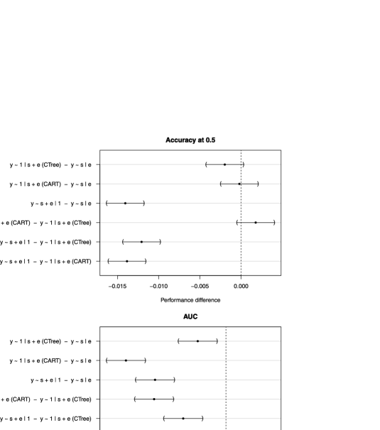
However, the differences among the models employing the combined set themselves (especially between the global logistic regression model and partitioned models) are not that strong. Therefore, to establish a region of performance differences that could be expected if all models performed equally well, we calculated simultaneous $95\%$-confidence intervals of all pairwise performance differences between the models that use the combined set of variables based on their accuracy as well as AUC. The former can be found in the upper panel of Figure 5, the latter in the lower panel. We can see that the global logistic regression model performs significantly worse than the partitioned models ($\alpha=0.05$). The tree methods perform best in terms of accuracy and their intervals overlap. In contrast, in terms of the cutoff free measure AUC, the $y\sim s|e$ LORET significantly outperforms all other methods.

4.5 Voter segmentation (“Voter profiles”).

“Voter profiles” are descriptions of a voter or set of voters that may include demographic, geographic and psychographic characteristics, as well as voting patterns and voting history. Voter profiles are popular in targeting efforts by campaigns, as they allow to break the complexity of all the available data down into a small number of key characteristics that can easily be acted upon. Key demographic variables are gender, income, age and education. A famous example of a voter profile is the “soccer mom” [Susan (1999)].

Multivariate voter profiles arise naturally from the LORET framework and the resulting profiles have two distinct benefits: On the one hand, the voter profiles are automatically created by a data-driven procedure, as tree-based methods algorithmically segment the data into mutually exclusive subsets. The segmentation is based on predictor variables in a well-defined fashion and the selection of important predictors is (usually) done automatically. On the other hand, logistic regression and trees with logistic node models are able to express an individual probability for each voter to turn up at the polls by including regressor variables in the logistic model and thus further differentiate the predicted probability between people in a segment. This way logistic regressions and model trees can provide individual predictions rather than a single prediction for a given profile. Furthermore, the estimates of the logistic model and/or the decision rules of the trees offer additional insight into the dynamics of voting behavior.

As case in point, consider the most general LORET, $y\sim s|e$. We have shown in the previous section that it has high accuracy and AUC for this data set. To derive voter profiles based on this model, we fit the logistic regression tree to the whole data set. The decision rules for building the segments and the coefficients for the logistic regression model in each terminal node can be found in Table 5.

We can see that the segmentation is driven by only four variables, the party composition of the household for each voter (“partyMix”), the relative frequency of attended elections (“attendance”), the rank of the individual in the household (“hhRank,” with “1” being highest and “3$+$” being lowest) and whether the person is the head (“H”) or a member (“M”) of the household (“hhHead”). Hence, most partitioning variables are concerned with the household structure rather than with individual-level variables. This underlines a streak of literature that emphasizes the importance of the household for voting behavior [e.g., Cutts and Fieldhouse (2009)].

= Partitioning variables Regressor variables Segment partyMix attend. hhRank hhHead const. gen00 gen01 gen02 gen03 ppp04 age $\bolds{\mathrm{age}^{2}}\bolds{\cdot 100}$ 2 unknown – – – $-\infty$ $0.000$ $0.000$ $0.000$ $0.000$ $0.000$ $0.000$ $0.000$ (–.–) (–.–) (–.–) (–.–) (–.–) (–.–) (–.–) (–.–) 6 allD $\leq$0.48 – – $0.508$ $0.840$ $-1.474$ $0.287$ $-0.750$ $0.442$ $0.054$ $-0.038$ $(0.623)$ $(0.269)$ $(0.212)$ $(0.212)$ $(0.212)$ $(0.231)$ $(0.024)$ $(0.022)$ 7 allR, onlyRorD $\leq$0.48 – – $0.427$ $0.740$ $-0.465$ $0.756$ $-0.075$ $0.708$ $0.011$ $-0.004$ $(0.660)$ $(0.239)$ $(0.174)$ $(0.185)$ $(0.177)$ $(0.169)$ $(0.028)$ $(0.027)$ 8 allR, allD, $>$0.48 – – $2.760$ $0.277$ $-1.164$ $0.352$ $-1.890$ $-0.952$ $0.035$ $-0.017$ onlyRorD $(0.948)$ $(0.339)$ $(0.352)$ $(0.379)$ $(0.604)$ $(0.354)$ $(0.025)$ $(0.021)$ 10 noneRorD, noneD, – – 3$+$ $4.057$ $0.781$ $0.591$ $1.249$ $1.520$ $0.677$ $-0.250$ $0.272$ noneR, legal $(0.797)$ $(0.128)$ $(0.203)$ $(0.165)$ $(0.214)$ $(0.212)$ $(0.052)$ $(0.076)$ 12 noneRorD, noneD, – $<\!3+$ H $-3.630$ $1.415$ $-0.010$ $1.521$ $2.218$ $1.694$ $0.116$ $-0.108$ noneR, legal $(0.339)$ $(0.079)$ $(0.111)$ $(0.105)$ $(0.167)$ $(0.223)$ $(0.013)$ $(0.012)$ 13 noneRorD, noneD, – $<\!3+$ M $-1.868$ $1.217$ $0.086$ $1.081$ $1.700$ $1.603$ $0.079$ $-0.078$ noneR, legal $(0.428)$ $(0.113)$ $(0.148)$ $(0.133)$ $(0.193)$ $(0.262)$ $(0.019)$ $(0.021)$

Table 5: A tabular representation of the terminal nodes for the $y\sim s|e$ LORET for the whole Ohio voter data set. The first column lists the terminal node numbers. The next four columns list the partitioning variables (party mix, attendance, household rank and household head) and the split point (if any). The last eight columns list the coefficients (upper row) and standard errors (lower row) for the fitted logistic models in the nodes. Please note that the values for the quadratic effect of age have been multiplied by 100 for readability.

Note that none of the commonly used demographic variables like gender, education or income plays a role in our tree. We therefore have voter profiles that suggest to look at whether a person comes from a household where all members are Democrats, all members are Republican or Democrats or a combination of both, or unknown composition, and all with potentially unaffiliated voters in the household. Additionally, our model suggests that one needs to consider the rank of each person in the household and how often the person went voting in the past. The segmentation then gives rise to different logistic models that provide additional targeting suggestions for a campaign based on the coefficients (cf. Table 5 and the predicted probabilities of each individual person in Table 6).

The results of the segmentation can be used to build more refined voter profiles by looking at the marginal distribution of different variables as displayed in Figure 6. These profiles also allow to derive strategic implications for a targeting campaign. For instance, for all individuals for whom “partyMix” is unknown (segment 2), we find the predicted probability to vote is near zero [actually a case where for a linear combination of predictors we have only one level of the outcome, or quasi-complete separation, Albert and Anderson (1984)]. We further see that people in this segment are mostly independent voters (78.6%), relatively often between 19 and 36 year-old individuals (29%), have a secondary education (62.4%) and earn between 35,000 and 75,000 USD a year (47.2%).

Table 6: An example for a targeting list based on predicted probabilities of 10 randomly selected individuals for the $y\sim s+e$ LORET of the Ohio voter data file

					Abs. freq.	Rel. freq.
$\bolds{\hat{\pi}_{i}}$	Segment	Age	Income	Education	votes	votes	Gender	Party
1.00	$13$	60.02	D	C	$6.00$	0.14	F	R
0.95	$12$	44.54	E	D	$4.00$	0.15	M	U
0.93	$7$	63.42	D	B	$21.00$	0.48	F	R
0.92	$13$	51.30	I	E	$14.00$	0.32	F	U
0.88	$8$	22.97	C	D	$7.00$	0.50	F	D
0.52	$14$	27.03	C	B	$3.00$	0.12	F	U
0.44	$14$	30.24	E	B	$1.00$	0.07	F	U
0.41	$13$	25.64	F	C	$3.00$	0.00	F	U
0.18	$12$	23.69	D	B	$0.00$	0.00	F	U
0.00	$2$	47.39	F	C	$1.00$	0.12	F	U

The most likely voters can be found in segment 7 (mean and median predicted voting probability of $0.908$ and $0.925$, resp.) and 13 (mean and median predicted probability of $0.861$ and $0.939$, resp.). Segment 7 has the highest percentage of likely voters (99%, see Figure 6) and consists of people who come from households that either are comprised only of Republicans or of both Republicans and Democrats and who went voting less than 48% of the times. The people in this segment are most often between 36 and 46 years of age (33.7%) or older than 55 (29.4%), declared Republican voters (88.9%) and often head of a household (56.6%). With 32.2%, segment 7 has the highest proportion of people with high income (more than 75,000 USD a year) compared to all other segments. In Segment 13 are people from households with at least one, but predominantely only unaffiliated voters in the household and whose household rank is 2. Roughly three quarters (72%) in this segment are women. Together with the household rank of 2 this points toward this being a segment of spouses or partners (typically wives). The most frequent age group in this segment is 46–54 (31.1%). Age has an interesting differential effect in these two segments of likely voters: When looking at the coefficients of the logistic regression model—recall that we specified a quadratic effect—we see that for segment 7 the turning point is at a high age of 70, but for segment 13 it already appears at 51.1 years.

Figure 6: Spineplots of the marginal distribution of important voter profile variables for all segments (the segment number is on the $x$-axis). The variables are vote (a categorization of the predicted voting probability: “likely” $(0.7,1]$, “undecided” $(0.3,0.7]$, “unlikely” $[0,0.3]$), party affiliation (“D” for Democrat, “R” for Republican and “U” for unaffiliated/independent), gender (“M” for male, “F” for female), education level (“primary,” “secondary,” “postsec”), yearly income (“$<$35k,” “35k–75k” and “$>$75k”) and age category.

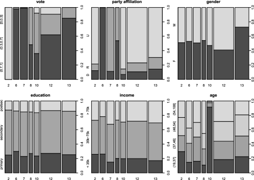
With respect to the mobilization of voters who are undecided as to whether they will turnout, segments 10 and 8 are most interesting. As the top left panel in Figure 6 shows, segment 10 is the segment with the highest proportion of “undecided” voters (56.04%). These voters are from a household with at least one independent or unaffiliated member and have a household rank of 3 or more. This segment is special insofar as it contains nearly exclusively young people (between 19 and 26, 91.2%) that describe themselves as unaffiliated voters (85.5%). This segment consists of the highest proportion of people with post-secondary education (16.3%). It collects young, unaffiliated voters whose predicted probabilities fall into the targeting range in more than 50% of the cases. In contrast, the second “undecided” segment, segment 8 (51.7% undecided), is characterized by people who are supporters of either the Republican or the Democratic Party in near equal numbers. Additionally, this segment has the highest proportion of elderly voters (44.7% are over 55). This segment would best be described as elderly, partisan voters who tend to be predicted as being undecided.

As an alternative to the aggregated view with voter profiles, a campaign can also use the nonaggregated predicted probabilities by generating a turnout or support probability for each voter in the database. Table 6 shows an example with 10 randomly chosen individuals. We list their predicted probabilities together with the according realizations of some additional variables. With such a list it is up to the individual campaign to decide how they eventually want to rank the individuals based on the probabilities and how to slice-and-dice these lists. In our campaign, where we want to include only those people in the targeting range of $[0.3,0.7]$, we would consider persons 6, 7 and 8. If the campaigns would have plans to additionally target only those that were younger than 30, then persons 6 and 8 would be targeted.

5 Conclusions.

In this paper a framework of statistical methods for targeting for turnout or targeting for support of eligible voters has been proposed. It combines ideas of trees with the idea of logistic regression which was coined LORET. The predictive accuracy performance of different specifications of LORET estimated with different algorithms has been investigated for an exemplary data set in a “targeting for turnout” setting for a typical situation that a campaign can face: having a reliable proxy for the target variable at its disposal. Furthermore, we illustrated how the creation of data-driven voter profiles arises naturally in the LORET framework and how this can be used for targeting.

The framework generalizes approaches used by campaigns and is easy to understand or communicate to people who are familiar with logistic regression and/or trees. Furthermore, it allows to create a segmentation of the data which corresponds to automatically building data-driven voter profiles which can enhance the effectiveness of targeting measures. As such, the framework is well suited for the purpose of segmentation and identification in voter targeting.

Regarding the special cases of LORET, a tree with a logistic node model may be the most useful default version. For our data, it has the best cutoff independent predictive accuracy (measured by AUC) and the highest predictive accuracy (at a cutoff of $0.5$). Please note that in our study we had completely accurate labels available, so the accuracy to be expected when dealing only with a proxy from polls might easily be lower. The logistic model tree has the additional advantage of providing refined voter profiles for targeting. As a result, decisions based on the $y\sim s|e$ LORET are easy to communicate to campaigns that already use logistic regression or trees.

The other instances of LORET, however, are not without merit either. Specifically, a LORET of the $y\sim 1|s+e$ type is a good choice if it is not clear what the functional form in the nodes should look like or if there is no standard set of variables to be used in the terminal nodes. Here the nonparametric nature of classification trees show their advantage. If the targeting situation is such that the proxies are generally not very reliable/typical for the real outcome of interest or there is a high degree of noise in these variables, the extra flexibility and tendency to overfit which trees exhibit can be a disadvantage. Here, logistic regression may be more appropriate due to the strict functional relationship that it imposes and therefore exhibiting less variability in the predictions about the future. Therefore, even a LORET with just a root node can come in handy.

We find that if campaigns can use accurate proxy data for the outcome of interest, the flexibility introduced by the tree structure may lead to higher predictive accuracy. In a situation where the campaign has to rely on historic proxy data for the outcome of interest, the predictive accuracy is generally low and there will probably be little difference between using a single logistic model or learning partitions as well (see the rejoinder in the supplementary material [Rusch et al. (2013b)]). We conclude that campaigns are generally best advised to make an effort in collecting accurate proxies for the outcome of interest and enabling an analysis as outlined in Section 4.4. We believe this is feasible by using well-designed, repeated polling to obtain the target variable. It is up to future research to establish what the best proxies to be used as labels in the targeting stage actually are.

With the benefits mentioned above, one would consider how to incorporate this technique into the overall campaign strategy. The primary benefit of using our framework is that campaigns can have accurate, interpretable, specific individual level identification of potential voters. This gives campaigns the ability to customize communications to each individual. Once the campaigns have better knowledge of the potential voter profiles and the likelihood of them voting, campaigns can maximize the return for the money spent on targeting potential voters by communicating on issues that matter to them and target voters who are likely to be mobilized. The bottom line here is that the LORET framework does not change the commonly used campaign tactics but adds a precise and flexible tool that allows to segment and target the recipients of mobilization messages accurately. For example, in the decision theoretic framework of optimal campaigning by Imai and Strauss (2011), LORET models that employ segmentation could be used as the building block for estimating heterogenous treatment effects to yield the posterior distributions of the turnout profiles [i.e., in steps 1 to 3 of Imai and Strauss (2011), page 9]. We believe that by employing the LORET framework, campaigns have a flexible and versatile toolbox at their disposal that can be customized to meet the campaign’s prevalent requirements and can easily be integrated in the overall strategy of GOTV targeting.

For further research and practical application, it could be fruitful to improve aspects of particular interest in GOTV campaigns. For example, it might be beneficial to use techniques such as artificial neural networks or ensembles of tree methods to improve predictive accuracy. Over the course of this study we used random forests, neural networks, support vector machines, Bayesian additive regression trees and logistic model trees with boosting to check whether they outperform our tree models. On our data set their performance was not better than the performance of the LORET models, so we refrained from investigating those techniques further and reporting them here (but see the supplementary material [Rusch et al. (2013b)]). Regularized logistic regression models might prove to be a sensible alternative to the tree approach, especially in terms of interpretability and variable selection. Regarding the node models, semi- or nonparametric models might be of interest as well, especially when the functional form for the logistic model component is not clear. For building voter profiles based on a predictive model, mixture models might also be an interesting alternative.

Appendix: Computational Details.

All calculations have been carried out with the statistical software R 2.12.0–2.15.2 [R Development Core Team (2012)], using glm() for logistic regression. Recursive partitioning infrastructure was provided by the packages party for mob() [Zeileis, Hothorn and Hornik (2008)] (with safeGLModel from mobtools, Rusch et al. (2012)] and ctree() [Hothorn, Hornik and Zeileis (2006)], as well as rpart [Therneau and Atkinson (1997), Therneau, Atkinson and Ripley (2011)] for CART. We used the ROCR package [Sing et al. (2005, 2009)] for calculating and plotting performance measures and ROC curves and multcomp [Hothorn, Bretz and Westfall (2008)] for the simultaneous confidence intervals.

References

- Albert and Anderson (1984) {barticle}[mr] \bauthor\bsnmAlbert, \bfnmA.\binitsA. and \bauthor\bsnmAnderson, \bfnmJ. A.\binitsJ. A. (\byear1984). \btitleOn the existence of maximum likelihood estimates in logistic regression models. \bjournalBiometrika \bvolume71 \bpages1–10. \biddoi=10.1093/biomet/71.1.1, issn=0006-3444, mr=0738319 \bptokimsref \endbibitem
- Arceneaux and Nickerson (2009) {barticle}[author] \bauthor\bsnmArceneaux, \bfnmK.\binitsK. and \bauthor\bsnmNickerson, \bfnmD. W.\binitsD. W. (\byear2009). \btitleWho is mobilized to vote? A re-analysis of 11 field experiments. \bjournalAmerican Journal of Political Science \bvolume53 \bpages1–16. \bptokimsref \endbibitem
- Blumenthal (2012) {bmisc}[author] \bauthor\bsnmBlumenthal, \bfnmM.\binitsM. (\byear2012). \bhowpublishedObama campaign polls: How the internal data got it right. Huffington Post. Available at http://www.huffingtonpost.com/2012/11/21/obama- campaign-polls-2012_n_2171242.html?utm_hp_ref=tw [accessed 2012-12-09]. \bptokimsref \endbibitem
- Breiman et al. (1984) {bbook}[author] \bauthor\bsnmBreiman, \bfnmL.\binitsL., \bauthor\bsnmFriedman, \bfnmJ. H.\binitsJ. H., \bauthor\bsnmOlsen, \bfnmR. A.\binitsR. A. and \bauthor\bsnmStone, \bfnmC. J.\binitsC. J. (\byear1984). \btitleClassification and Regression Trees. \bpublisherWadsworth, \blocationPacific Grove, CA. \bptokimsref \endbibitem
- Cardy (2005) {barticle}[author] \bauthor\bsnmCardy, \bfnmE. A.\binitsE. A. (\byear2005). \btitleAn experimental field study and persuasion effects of partisan direct mail and phone calls. \bjournalAnnals of the American Academy of Political and Social Science \bvolume601 \bpages28–40. \bptokimsref \endbibitem
- Chan and Loh (2004) {barticle}[mr] \bauthor\bsnmChan, \bfnmKin-Yee\binitsK.-Y. and \bauthor\bsnmLoh, \bfnmWei-Yin\binitsW.-Y. (\byear2004). \btitleLOTUS: An algorithm for building accurate and comprehensible logistic regression trees. \bjournalJ. Comput. Graph. Statist. \bvolume13 \bpages826–852. \biddoi=10.1198/106186004X13064, issn=1061-8600, mr=2109054 \bptokimsref \endbibitem
- Chaudhuri et al. (1995) {barticle}[mr] \bauthor\bsnmChaudhuri, \bfnmProbal\binitsP., \bauthor\bsnmLo, \bfnmWen Da\binitsW. D., \bauthor\bsnmLoh, \bfnmWei-Yin\binitsW.-Y. and \bauthor\bsnmYang, \bfnmChing Ching\binitsC. C. (\byear1995). \btitleGeneralized regression trees. \bjournalStatist. Sinica \bvolume5 \bpages641–666. \bidissn=1017-0405, mr=1347613 \bptokimsref \endbibitem
- Chipman, George and McCulloch (2010) {barticle}[mr] \bauthor\bsnmChipman, \bfnmHugh A.\binitsH. A., \bauthor\bsnmGeorge, \bfnmEdward I.\binitsE. I. and \bauthor\bsnmMcCulloch, \bfnmRobert E.\binitsR. E. (\byear2010). \btitleBART: Bayesian additive regression trees. \bjournalAnn. Appl. Stat. \bvolume4 \bpages266–298. \biddoi=10.1214/09-AOAS285, issn=1932-6157, mr=2758172 \bptokimsref \endbibitem
- Cutts and Fieldhouse (2009) {barticle}[author] \bauthor\bsnmCutts, \bfnmD.\binitsD. and \bauthor\bsnmFieldhouse, \bfnmE.\binitsE. (\byear2009). \btitleWhat small spatial scales are relevant as electoral contexts for individual voters? The importance of the household on turnout at the 2001 general election. \bjournalAmerican Journal of Political Science \bvolume53 \bpages726–739. \bptokimsref \endbibitem
- Denny and Doyle (2009) {barticle}[author] \bauthor\bsnmDenny, \bfnmK.\binitsK. and \bauthor\bsnmDoyle, \bfnmO.\binitsO. (\byear2009). \btitleDoes voting history matter? Analysing persistence in turnout. \bjournalAmerican Journal of Political Science \bvolume53 \bpages17–35. \bptokimsref \endbibitem
- Finkel (1993) {barticle}[author] \bauthor\bsnmFinkel, \bfnmSteven\binitsS. (\byear1993). \btitleReexamining the “Minimal effects” model in recent presidential elections. \bjournalJournal of Politics \bvolume55 \bpages1–21. \bptokimsref \endbibitem
- Gerber and Green (2000a) {barticle}[author] \bauthor\bsnmGerber, \bfnmA. S.\binitsA. S. and \bauthor\bsnmGreen, \bfnmD. P.\binitsD. P. (\byear2000a). \btitleThe effect of a nonpartisan get-out-the-vote drive: An experimental study of leafleting. \bjournalJournal of Politics \bvolume62 \bpages846–857. \bptokimsref \endbibitem
- Gerber and Green (2000b) {barticle}[author] \bauthor\bsnmGerber, \bfnmAllan S.\binitsA. S. and \bauthor\bsnmGreen, \bfnmDonald P.\binitsD. P. (\byear2000b). \btitleThe effects of canvassing, telephone calls, and direct mail on voter turnout: A field experiment. \bjournalAmerican Political Science Review \bvolume94 \bpages656–664. \bptokimsref \endbibitem
- Gerber, Green and Green (2007) {barticle}[author] \bauthor\bsnmGerber, \bfnmA. S.\binitsA. S., \bauthor\bsnmGreen, \bfnmD. P.\binitsD. P. and \bauthor\bsnmGreen, \bfnmM.\binitsM. (\byear2007). \btitlePartisan mail and voter turnout: Results from randomized field experiments. \bjournalElectoral Studies \bvolume22 \bpages563–579. \bptokimsref \endbibitem
- Goldstein and Ridout (2002) {barticle}[author] \bauthor\bsnmGoldstein, \bfnmK.\binitsK. and \bauthor\bsnmRidout, \bfnmT. N.\binitsT. N. (\byear2002). \btitleThe politics of participation: Mobilization and turnout over time. \bjournalPolitical Behavior \bvolume24 \bpages3–29. \bptokimsref \endbibitem
- Green, Gerber and Nickerson (2003) {barticle}[author] \bauthor\bsnmGreen, \bfnmD. P.\binitsD. P., \bauthor\bsnmGerber, \bfnmA. S.\binitsA. S. and \bauthor\bsnmNickerson, \bfnmD. W.\binitsD. W. (\byear2003). \btitleGetting out the vote in local elections: Results from six door-to-door canvassing experiments. \bjournalJournal of Politics \bvolume65 \bpages1083–1096. \bptokimsref \endbibitem
- Green and Gerber (2008) {bbook}[author] \bauthor\bsnmGreen, \bfnmD. P.\binitsD. P. and \bauthor\bsnmGerber, \bfnmA. S.\binitsA. S. (\byear2008). \btitleGet Out the Vote: How to Increase Voter Turnout, \bedition2nd ed. \bpublisherBrookings Institution, \blocationWashington DC. \bptokimsref \endbibitem
- Green and Kern (2012) {barticle}[author] \bauthor\bsnmGreen, \bfnmD. P.\binitsD. P. and \bauthor\bsnmKern, \bfnmH. L.\binitsH. L. (\byear2012). \btitleModeling heterogeneous treatment effects in survey experiments with Bayesian additive regression trees. \bjournalPublic Opinion Quarterly \bvolume76 \bpages491–511. \bptokimsref \endbibitem
- Hansen and Bowers (2009) {barticle}[mr] \bauthor\bsnmHansen, \bfnmBen B.\binitsB. B. and \bauthor\bsnmBowers, \bfnmJake\binitsJ. (\byear2009). \btitleAttributing effects to a cluster-randomized get-out-the-vote campaign. \bjournalJ. Amer. Statist. Assoc. \bvolume104 \bpages873–885. \biddoi=10.1198/jasa.2009.ap06589, issn=0162-1459, mr=2562000 \bptokimsref \endbibitem
- Hastie, Tibshirani and Friedman (2009) {bbook}[mr] \bauthor\bsnmHastie, \bfnmTrevor\binitsT., \bauthor\bsnmTibshirani, \bfnmRobert\binitsR. and \bauthor\bsnmFriedman, \bfnmJerome\binitsJ. (\byear2009). \btitleThe Elements of Statistical Learning: Data Mining, Inference, and Prediction, \bedition2nd ed. \bpublisherSpringer, \blocationNew York. \biddoi=10.1007/978-0-387-84858-7, mr=2722294 \bptokimsref \endbibitem
- Holbrook and McClurg (2005) {barticle}[author] \bauthor\bsnmHolbrook, \bfnmT. M.\binitsT. M. and \bauthor\bsnmMcClurg, \bfnmS. D.\binitsS. D. (\byear2005). \btitleThe mobilization of core supporters: Campaigns, turnout and electoral composition in United States presidential elections. \bjournalAmerican Journal of Political Science \bvolume49 \bpages689–703. \bptokimsref \endbibitem
- Hothorn, Bretz and Westfall (2008) {barticle}[mr] \bauthor\bsnmHothorn, \bfnmTorsten\binitsT., \bauthor\bsnmBretz, \bfnmFrank\binitsF. and \bauthor\bsnmWestfall, \bfnmPeter\binitsP. (\byear2008). \btitleSimultaneous inference in general parametric models. \bjournalBiom. J. \bvolume50 \bpages346–363. \biddoi=10.1002/bimj.200810425, issn=0323-3847, mr=2521547 \bptokimsref \endbibitem
- Hothorn, Hornik and Zeileis (2006) {barticle}[mr] \bauthor\bsnmHothorn, \bfnmTorsten\binitsT., \bauthor\bsnmHornik, \bfnmKurt\binitsK. and \bauthor\bsnmZeileis, \bfnmAchim\binitsA. (\byear2006). \btitleUnbiased recursive partitioning: A conditional inference framework. \bjournalJ. Comput. Graph. Statist. \bvolume15 \bpages651–674. \biddoi=10.1198/106186006X133933, issn=1061-8600, mr=2291267 \bptokimsref \endbibitem
- Hothorn et al. (2005) {barticle}[mr] \bauthor\bsnmHothorn, \bfnmTorsten\binitsT., \bauthor\bsnmLeisch, \bfnmFriedrich\binitsF., \bauthor\bsnmZeileis, \bfnmAchim\binitsA. and \bauthor\bsnmHornik, \bfnmKurt\binitsK. (\byear2005). \btitleThe design and analysis of benchmark experiments. \bjournalJ. Comput. Graph. Statist. \bvolume14 \bpages675–699. \biddoi=10.1198/106186005X59630, issn=1061-8600, mr=2170208 \bptokimsref \endbibitem
- Imai and Strauss (2011) {barticle}[author] \bauthor\bsnmImai, \bfnmK.\binitsK. and \bauthor\bsnmStrauss, \bfnmA.\binitsA. (\byear2011). \btitleEstimation of heterogeneous treatment effects from randomized experiments, with application to the optimal planning of the get-out-the-vote campaign. \bjournalPolitical Analysis \bvolume19 \bpages1–19. \bptokimsref \endbibitem
- Issenberg (2012a) {bmisc}[author] \bauthor\bsnmIssenberg, \bfnmSasha\binitsS. (\byear2012a). \bhowpublishedObama’s white whale: How the campaign’s top-secret project Narwhal could change this race, and many to come. Slate. Available at http://www.slate.com/articles/news_and_politics/victory_lab/2012/02/project_ narwhal_how_a_top_secret_obama_campaign_program_could_change_the_2012_race_.html [accessed 2012-12-04]. \bptokimsref \endbibitem
- Issenberg (2012b) {bbook}[author] \bauthor\bsnmIssenberg, \bfnmSasha\binitsS. (\byear2012b). \btitleThe Victory Lab: The Secret Science of Winning Campaigns. \bpublisherCrown Publishers, \blocationNew York. \bptokimsref \endbibitem
- Karp and Banducci (2007) {barticle}[author] \bauthor\bsnmKarp, \bfnmJ. A.\binitsJ. A. and \bauthor\bsnmBanducci, \bfnmS. A.\binitsS. A. (\byear2007). \btitleParty mobilization and political participation in new and old democracies. \bjournalParty Politics \bvolume13 \bpages217–234. \bptokimsref \endbibitem
- Karp, Banducci and Bowler (2008) {barticle}[author] \bauthor\bsnmKarp, \bfnmJ. A.\binitsJ. A., \bauthor\bsnmBanducci, \bfnmS. A.\binitsS. A. and \bauthor\bsnmBowler, \bfnmS.\binitsS. (\byear2008). \btitleGetting out the vote: Party mobilization in a comparative perspective. \bjournalBritish Journal of Political Science \bvolume38 \bpages91–112. \bptokimsref \endbibitem
- Kass (1980) {barticle}[author] \bauthor\bsnmKass, \bfnmG. V.\binitsG. V. (\byear1980). \btitleAn exploratory technique for investigating large quantities of categorical data. \bjournalJ. R. Stat. Soc. Ser. C. Appl. Stat. \bvolume29 \bpages119–127. \bptokimsref \endbibitem
- Landwehr, Hall and Eibe (2005) {barticle}[author] \bauthor\bsnmLandwehr, \bfnmN.\binitsN., \bauthor\bsnmHall, \bfnmM.\binitsM. and \bauthor\bsnmEibe, \bfnmF.\binitsF. (\byear2005). \btitleLogistic model trees. \bjournalMachine Learning \bvolume59 \bpages161–205. \bptokimsref \endbibitem
- Loh and Shih (1997) {barticle}[mr] \bauthor\bsnmLoh, \bfnmWei-Yin\binitsW.-Y. and \bauthor\bsnmShih, \bfnmYu-Shan\binitsY.-S. (\byear1997). \btitleSplit selection methods for classification trees. \bjournalStatist. Sinica \bvolume7 \bpages815–840. \bidissn=1017-0405, mr=1488644 \bptokimsref \endbibitem
- Malchow (2008) {bbook}[author] \bauthor\bsnmMalchow, \bfnmH.\binitsH. (\byear2008). \btitlePolitical Targeting, \bedition2nd ed. \bpublisherPredicted Lists, LLC, \blocationSacramento, CA. \bptokimsref \endbibitem
- McCullagh and Nelder (1989) {bbook}[author] \bauthor\bsnmMcCullagh, \bfnmPeter\binitsP. and \bauthor\bsnmNelder, \bfnmJohn A.\binitsJ. A. (\byear1989). \btitleGeneralized Linear Models, \bedition2nd ed. \bpublisherChapman & Hall, \blocationNew York. \bptokimsref \endbibitem
- McDonald (2012) {bmisc}[author] \bauthor\bsnmMcDonald, \bfnmMichael\binitsM. (\byear2012). \bhowpublishedTurnout rates, 1980–2010. United States Election Project. Available at http://elections.gmu.edu/ [accessed 2012-02-16]. \bptokimsref \endbibitem
- Muller (1999) {barticle}[author] \bauthor\bsnmMuller, \bfnmM. G.\binitsM. G. (\byear1999). \btitleElectoral campaigning as an occupation—The professionalization of political consultants in the United States. \bjournalPolitische Vierteljahresschrift \bvolume40 \bpages198–199. \bptokimsref \endbibitem
- Murray and Scime (2010) {barticle}[author] \bauthor\bsnmMurray, \bfnmGregg R.\binitsG. R. and \bauthor\bsnmScime, \bfnmAnthony\binitsA. (\byear2010). \btitleMicrotargeting and electorate segmentation: Data mining the American national election studies. \bjournalJournal of Political Marketing \bvolume9 \bpages143–166. \bptokimsref \endbibitem
- Nickerson, Friedrichs and King (2006) {barticle}[author] \bauthor\bsnmNickerson, \bfnmD. W.\binitsD. W., \bauthor\bsnmFriedrichs, \bfnmR. D.\binitsR. D. and \bauthor\bsnmKing, \bfnmD. C.\binitsD. C. (\byear2006). \btitlePartisan mobilization campaigns in the field: Results from a statewide turnout experiment in Michigan. \bjournalPolitical Research Quarterly \bvolume59 \bpages85–97. \bptokimsref \endbibitem
- Panagopoulos (2009) {barticle}[author] \bauthor\bsnmPanagopoulos, \bfnmC.\binitsC. (\byear2009). \btitlePartisan and nonpartisan message content and voter mobilization field experimental evidence. \bjournalPolitical Research Quarterly \bvolume62 \bpages70–76. \bptokimsref \endbibitem
- Parry et al. (2008) {barticle}[author] \bauthor\bsnmParry, \bfnmJ.\binitsJ., \bauthor\bsnmBarth, \bfnmJ.\binitsJ., \bauthor\bsnmKropf, \bfnmM.\binitsM. and \bauthor\bsnmJones, \bfnmE. T.\binitsE. T. (\byear2008). \btitleMobilizing the seldom voter: Campaign contact and effects in high-profile elections. \bjournalPolitical Behavior \bvolume30 \bpages97–113. \bptokimsref \endbibitem
- Phillips, Urbany and Reynolds (2008) {barticle}[author] \bauthor\bsnmPhillips, \bfnmJ. M.\binitsJ. M., \bauthor\bsnmUrbany, \bfnmJ. E.\binitsJ. E. and \bauthor\bsnmReynolds, \bfnmT. J.\binitsT. J. (\byear2008). \btitleConfirmation and the effects of valenced political advertising: A field experiment. \bjournalJournal of Consumer Research \bvolume34 \bpages794–806. \bptokimsref \endbibitem
- Plasser (2000) {barticle}[author] \bauthor\bsnmPlasser, \bfnmF.\binitsF. (\byear2000). \btitleAmerican campaign techniques worldwide. \bjournalHarvard International Journal of Press-Politics \bvolume5 \bpages33–54. \bptokimsref \endbibitem
- Quinlan (1993) {bbook}[author] \bauthor\bsnmQuinlan, \bfnmJ. R.\binitsJ. R. (\byear1993). \btitleC4.5: Programs for Machine Learning. \bpublisherMorgan Kaufmann, \blocationSan Mateo, CA. \bptokimsref \endbibitem
- R Development Core Team (2012) {bmisc}[author] \borganizationR Development Core Team (\byear2012). \bhowpublishedR: A language and environment for statistical computing. R Foundation for Statstical Computing, Vienna, Austria. \bptokimsref \endbibitem
- Rusch and Zeileis (2013) {barticle}[author] \bauthor\bsnmRusch, \bfnmThomas\binitsT. and \bauthor\bsnmZeileis, \bfnmAchim\binitsA. (\byear2013). \btitleGaining insight with recursive partitioning of generalized linear models. \bjournalJ. Stat. Comput. Simul. \bvolume83 \bpages1301–1315. \bptokimsref \endbibitem
- Rusch et al. (2012) {bmisc}[author] \bauthor\bsnmRusch, \bfnmT.\binitsT., \bauthor\bsnmZeileis, \bfnmA.\binitsA., \bauthor\bsnmHothorn, \bfnmT.\binitsT. and \bauthor\bsnmLeisch, \bfnmF.\binitsF. (\byear2012). \bhowpublishedmobtools: A collection of statmodels and of utilities for extending mob. R package version 0.0-1. \bptokimsref \endbibitem
- Rusch et al. (2013a) {bmisc}[author] \bauthor\bsnmRusch, \bfnmThomas\binitsT., \bauthor\bsnmLee, \bfnmIlro\binitsI., \bauthor\bsnmHornik, \bfnmKurt\binitsK., \bauthor\bsnmJank, \bfnmWolfgang\binitsW. and \bauthor\bsnmZeileis, \bfnmAchim\binitsA. (\byear2013a). \bhowpublishedSupplement to “Influencing elections with statistics: Targeting voters with logistic regression trees.” DOI:\doiurl10.1214/13-AOAS648SUPPA. \bptokimsref \endbibitem
- Rusch et al. (2013b) {bmisc}[author] \bauthor\bsnmRusch, \bfnmThomas\binitsT., \bauthor\bsnmLee, \bfnmIlro\binitsI., \bauthor\bsnmHornik, \bfnmKurt\binitsK., \bauthor\bsnmJank, \bfnmWolfgang\binitsW. and \bauthor\bsnmZeileis, \bfnmAchim\binitsA. (\byear2013b). \bhowpublishedSupplement to “Influencing elections with statistics: Targeting voters with logistic regression trees.” DOI:\doiurl10.1214/13-AOAS648SUPPB. \bptokimsref \endbibitem
- Sing et al. (2005) {barticle}[pbm] \bauthor\bsnmSing, \bfnmTobias\binitsT., \bauthor\bsnmSander, \bfnmOliver\binitsO., \bauthor\bsnmBeerenwinkel, \bfnmNiko\binitsN. and \bauthor\bsnmLengauer, \bfnmThomas\binitsT. (\byear2005). \btitleROCR: Visualizing classifier performance in R. \bjournalBioinformatics \bvolume21 \bpages3940–3941. \biddoi=10.1093/bioinformatics/bti623, issn=1367-4803, pii=bti623, pmid=16096348 \bptokimsref \endbibitem
- Sing et al. (2009) {bmisc}[author] \bauthor\bsnmSing, \bfnmTobias\binitsT., \bauthor\bsnmSander, \bfnmOliver\binitsO., \bauthor\bsnmBeerenwinkel, \bfnmNiko\binitsN. and \bauthor\bsnmLengauer, \bfnmThomas\binitsT. (\byear2009). \bhowpublishedROCR: Visualizing the performance of scoring classifiers. R package version 1.0-4. \bptokimsref \endbibitem
- Susan (1999) {barticle}[author] \bauthor\bsnmSusan, \bfnmJ. C.\binitsJ. C. (\byear1999). \btitleThe disempowerment of the gender gap: Soccer moms and the 1996 elections. \bjournalPS: Political Science & Politics \bvolume32 \bpages7–11. \bptokimsref \endbibitem
- Sussman and Galizio (2003) {barticle}[author] \bauthor\bsnmSussman, \bfnmG.\binitsG. and \bauthor\bsnmGalizio, \bfnmL.\binitsL. (\byear2003). \btitleThe global reproduction of American politics. \bjournalPolitical Comunication \bvolume20 \bpages309–328. \bptokimsref \endbibitem
- Therneau and Atkinson (1997) {bmisc}[author] \bauthor\bsnmTherneau, \bfnmT. M.\binitsT. M. and \bauthor\bsnmAtkinson, \bfnmE. J.\binitsE. J. (\byear1997). \bhowpublishedAn introduction to recursive partitioning using the rpart routine. Technical Report 61, Section of Biostatistics, Mayo Clinic, Rochester, NY. \bptokimsref \endbibitem
- Therneau, Atkinson and Ripley (2011) {bmisc}[author] \bauthor\bsnmTherneau, \bfnmT. M.\binitsT. M., \bauthor\bsnmAtkinson, \bfnmE. J.\binitsE. J. and \bauthor\bsnmRipley, \bfnmBrian D.\binitsB. D. (\byear2011). \bhowpublishedrpart: Recursive partitioning. R package version 3.1-50. \bptokimsref \endbibitem
- US Election Assistance Commission (2010) {bmisc}[author] \borganizationUS Election Assistance Commission (\byear2010). \bhowpublishedThe Impact of the National Voter Registration Act of 1993 on the Administration of Elections for Federal Office 2009–2010. \bptokimsref \endbibitem
- Whitelock, Whitelock and van Heerde (2010) {barticle}[author] \bauthor\bsnmWhitelock, \bfnmA.\binitsA., \bauthor\bsnmWhitelock, \bfnmJ.\binitsJ. and \bauthor\bparticlevan \bsnmHeerde, \bfnmJ.\binitsJ. (\byear2010). \btitleThe influence of promotional activity and different electoral systems on voter turnout: A study of the UK and German Euro elections. \bjournalEuropean Journal of Marketing \bvolume44 \bpages401–420. \bptokimsref \endbibitem
- Wielhouwer (2003) {barticle}[author] \bauthor\bsnmWielhouwer, \bfnmPeter W.\binitsP. W. (\byear2003). \btitleIn search of Lincoln’s perfect list—Targeting in grassroots campaigns. \bjournalAmerican Politics Research \bvolume31 \bpages632–669. \bptokimsref \endbibitem
- Wikipedia (2012) {bmisc}[author] \borganizationWikipedia (\byear2012). \bhowpublishedUnited States presidential election, 2012. Available at http://en. wikipedia.org/wiki/Unite_States_presidential_election,_2012 [accessed 2012-11-21]. \bptokimsref \endbibitem
- Wilcoxon (1945) {barticle}[author] \bauthor\bsnmWilcoxon, \bfnmFrank\binitsF. (\byear1945). \btitleIndividual comparisons by ranking methods. \bjournalBiometrics Bulletin \bvolume1 \bpages80–83. \bptokimsref \endbibitem
- Zeileis, Hothorn and Hornik (2008) {barticle}[mr] \bauthor\bsnmZeileis, \bfnmAchim\binitsA., \bauthor\bsnmHothorn, \bfnmTorsten\binitsT. and \bauthor\bsnmHornik, \bfnmKurt\binitsK. (\byear2008). \btitleModel-based recursive partitioning. \bjournalJ. Comput. Graph. Statist. \bvolume17 \bpages492–514. \biddoi=10.1198/106186008X319331, issn=1061-8600, mr=2439970 \bptokimsref \endbibitem
- Zhang and Singer (2010) {bbook}[mr] \bauthor\bsnmZhang, \bfnmHeping\binitsH. and \bauthor\bsnmSinger, \bfnmBurton H.\binitsB. H. (\byear2010). \btitleRecursive Partitioning and Applications, \bedition2nd ed. \bpublisherSpringer, \blocationNew York. \biddoi=10.1007/978-1-4419-6824-1, mr=2674991 \bptokimsref \endbibitem