Simulation of cohesive fine powders under a plane shear

Abstract

Three dimensional molecular dynamics simulations of cohesive dissipative powders under a plane shear are performed. We find the various phases depending on the dimensionless shear rate and the dissipation rate as well as the density. We also find that the shape of clusters depends on the initial condition of velocities of particles when the dissipation is large. Our simple stochastic model reproduces the non-Gaussian velocity distribution function appearing in the coexistence phase of a gas and a plate.

I Introduction

Fine powders, such as aerosols, volcanic ashes, flours, and toner particles are commonly observed in daily life. The attractive interaction between fine powders plays major roles Krupp1967 ; Visser1989 ; Valverde2000 ; Tomas2001 ; Cansell2003 ; Tomas2004 ; Castellanos2005 ; Butt2005 ; Tykhoniuk2007 ; Tomas2007 ; Calvert2009 ; Israelachvili2011 ; Ommen2012 , while there are various studies discussing the effects of cohesive forces between macroscopic powders Derjaguin1956 ; Johnson1971 ; Derjaguin1975 ; Yen1992 ; Thornton1996 ; Hornbaker1997 ; Bocquet1998 ; Mikami1998 ; Nase2001 ; Israelachvili2011 ; Bartels2005 ; Willett2000 ; Herminghaus2005 ; Mitarai2006 ; Royer2009 ; Ulrich2012 ; Luding2003 ; Luding2005 ; Luding2008 ; Luding2014 ; Luding201407 . For example, the Johnson-Kendall-Roberts (JKR) theory describes microscopic surface energy for the contact of cohesive grains Johnson1971 ; Israelachvili2011 . The others study the attractive force caused by liquid bridge for wet granular particles Hornbaker1997 ; Bocquet1998 ; Willett2000 ; Nase2001 ; Herminghaus2005 ; Mitarai2006 ; Ulrich2012 . It should be noted that the cohesive force cannot be ignored for small fine powders. Indeed, the intermolecular attractive force always exists. Moreover, the inelasticity plays important roles when powders collide, because there are some excitations of internal vibrations, radiation of sounds, and deformations Gerl1999 ; Hayakawa2002 ; Awasthi2006 ; Brilliantov2007 ; Suri2008 ; Tanaka2012 ; Kuninaka2009 ; Kuninaka2012 ; Saitoh2010 ; Murakami2014 .
 Let us consider cohesive powders under a plane shear. So far there exist many studies for one or two effects of the shear, an attractive force, and an inelastic collision Saitoh2007 ; Yasuoka1998 ; Lasinski2004 ; Conway2004 ; Goldhirsch1993_1 ; Goldhirsch1993_2 ; McNamara1993 ; McNamara1996 ; Brilliantov2004 ; Hansen1969 ; Nicolas1979 ; Adachi1988 ; Lotfi1992 ; Johnson1993 ; Kolafa1993 ; Heist1994 ; Laaksonen1994 ; Alam2013 ; Shukla2013 , but we only know one example for the study of the jamming transition to include all three effects Gu2014 . On the other hand, when the Lennard-Jones (LJ) molecules are quenched below the coexistence curve of gas-liquid phases Hansen1969 ; Nicolas1979 ; Adachi1988 ; Lotfi1992 ; Johnson1993 ; Kolafa1993 , a phase ordering process proceeds after the nucleation takes place Heist1994 ; Laaksonen1994 ; Yasuoka1998 . It is well known that clusters always appear in freely cooling processes of granular gases Goldhirsch1993_1 ; Goldhirsch1993_2 ; McNamara1996 . Such clustering processes may be understood by a set of hydrodynamic equations of granular gases McNamara1993 ; Brilliantov2004 . When we apply a shear to the granular gas, there exist various types of clusters such as 2D plug, 2D wave, or 3D wave for three dimensional systems Lasinski2004 ; Conway2004 ; Saitoh2007 ; Alam2013 ; Shukla2013 .
 In this paper, we try to characterize nonequilibrium pattern formation of cohesive fine powders under the plane shear by the three dimensional molecular dynamics (MD) simulations of the dissipative LJ molecules under the Lees-Edwards boundary condition Lees1972 . In our previous paper Takada2013_2 , we have mainly focused on the effect of dissipation on the pattern formation in Sllod dynamics Evans1984 ; Evans2008 . In this study, we systematically study it by scanning a large area of parameters space to draw the phase diagrams with respect to the density, the dimensionless shear rate, and the dissipation rate without the influence of Sllod dynamics.
 The organization of this paper is as follows. In the next section, we introduce our model and setup for this study. Section III, the main part of this paper, is devoted to exhibit the results of our simulation. In Sec. III.1, we show the phase diagrams for several densities, each of which has various distinct steady phases. We find that the system has a quasi particle-hole symmetry. We also find that the steady states depend on the initial condition of velocities of particles when the dissipation is large. In Sec. III.2, we analyze the velocity distribution function, and try to reproduce it by solving the Kramers equation with Coulombic friction under the shear. In the last section, we discuss and summarize our results. In Appendix A, we study the pattern formation of dissipative LJ system under the physical boundary condition. In Appendix B, we illustrate the existence of Coulombic friction near the interface of the plate-gases coexistence phase. In Appendix C, we demonstrate that the viscous heating term near the interface is always positive. In Appendix D, we present a perturbative solution of the Kramers equation. In Appendix E, we show the detailed calculations for each moment. In Appendix F, we show the detailed calculations of the velocity distribution function.

II Molecular dynamics simulation

In this section, we explain our model and setup of MD for cohesive fine powders under a plane shear. We introduce our model of cohesive fine powders in Sec. II.1 and explain our numerical setup in Sec. II.2.

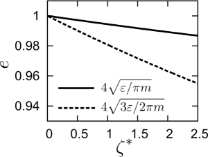
Figure 1: The relationship between the dimensionless dissipation rate $\zeta^{*}$ and the coefficient of restitution $e$ when the pre-collisional relative velocities (solid and dashed lines) are given by $4\sqrt{\varepsilon/\pi m}$ and $4\sqrt{3\varepsilon/2\pi m}$, respectively.

II.1 Model

We assume that the interaction between two cohesive fine powders can be described by LJ potential, and an inelastic force caused by collisions with finite relative speeds. The explicit expression of LJ potential is given by

$$U^{\rm LJ}(r_{ij})=4\varepsilon\Theta(r_{\rm c}-r_{ij})\left[\left(\frac{\sigma}{r_{ij}}\right)^{12}-\left(\frac{\sigma}{r_{ij}}\right)^{6}\right]$$ (1)

with a step function $\Theta(r)=1$ and $0$ for $r>0$ and $r\leq 0$, respectively, where $\varepsilon$, $\sigma$, and $r_{ij}$ are the well depth, the diameter of the repulsive core, and the distance between the particles $i$ and $j$, respectively. Here, we have introduced the cutoff length $r_{\rm c}=3.0\sigma$ to save the computational cost, i.e. $U^{\rm LJ}(r)=0$ for $r\geq r_{\rm c}$. To model the inelastic interaction, we introduce a viscous force between colliding two particles as

$$\bm{F}^{\rm vis}(\bm{r}_{ij},\bm{v}_{ij})=-\zeta\Theta(\sigma-r_{ij})(\bm{v}_{ij}\cdot\hat{\bm{r}}_{ij})\hat{\bm{r}}_{ij},$$ (2)

where $\zeta$, $\hat{\bm{r}}_{ij}\equiv\bm{r}_{ij}/r_{ij}$, and $\bm{v}_{ij}=\bm{v}_{i}-\bm{v}_{j}$ are the dissipation rate, a unit vector parallel to $\bm{r}_{ij}=\bm{r}_{i}-\bm{r}_{j}$, and the relative velocity between the particles, respectively. Here, $\bm{r}_{\alpha}$ and $\bm{v}_{\alpha}$ ($\alpha=i,j$) are, respectively, the position and velocity of the particle. It should be noted that the range of inelastic interaction is only limited within the distance $\sigma$. From Eqs. (1) and (2), the force acting on the $i$-th particle is given by

$$\bm{F}_{i}=-\sum_{j\neq i}\bm{\nabla}_{i}U^{\rm LJ}(r_{ij})+\sum_{j\neq i}\bm{F}^{\rm vis}(\bm{r}_{ij},\bm{v}_{ij}).$$ (3)

Our LJ model has an advantage to know the detailed properties in equilibrium Hansen1969 ; Nicolas1979 ; Adachi1988 ; Lotfi1992 ; Johnson1993 ; Kolafa1993 . The normal restitution coefficient $e$, defined as a ratio of post-collisional speed to pre-collisional speed, depends on both the dissipation rate $\zeta$ and incident speed. For instance, the particles are nearly elastic, i.e. the restitution coefficient, $e=0.994$ for the case of $\zeta=\sqrt{\varepsilon/m\sigma^{2}}$ and the incident speed $\sqrt{\varepsilon/m}$, where $m$ is the mass of each colliding particle. Figure 1 plots the restitution coefficient against the dimensionless dissipation rate $\zeta^{\ast}=\zeta\sqrt{m\sigma^{2}/\varepsilon}$, where the incident speeds are given by $4\sqrt{\varepsilon/\pi m}$ and $4\sqrt{3\varepsilon/2\pi m}$, respectively. We restrict the dissipation rate to small values in the range $0<\zeta^{\ast}\leq 3.2$. Note that small and not too large inelasticity is necessary to reproduce a steady coexistence phase between a dense and a dilute region, which will be analyzed in details in this paper. Indeed, the system cannot reach a steady state without inelasticity, while all particles are absorbed in a big cluster when inelasticity is large. In this paper, we use three dimensionless parameters to characterize a system: the dimensionless density $n^{*}=n\sigma^{3}=N\sigma^{3}/L^{3}$, the shear rate $\dot{\gamma}^{\ast}=\dot{\gamma}\sqrt{m\sigma^{2}/\varepsilon}$, and the dissipation rate $\zeta^{\ast}=\zeta\sqrt{m\sigma^{2}/\varepsilon}$. It should be noted that the well depth $\varepsilon$ is absorbed in the dimensionless shear rate and the dissipation rate. Thus, we may regard the control of two independent parameters as the change of the well depth.

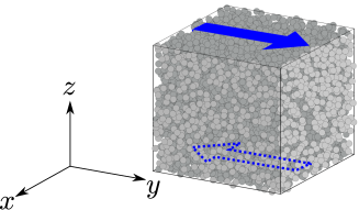
Figure 2: A snapshot of our simulation in a uniformly sheared state. We apply a plane shear in $xy$ plane, that is, we choose $y$-axis as the shear direction and $z$-axis as the velocity gradient direction.

II.2 Setup

Figure 2 is a snapshot of our MD for a uniformly sheared state, where we randomly distribute $N=10^{4}$ particles in a cubic periodic box and control the number density $n$ by adjusting the linear system size $L$. At first, we equilibrate the system by performing the MD with the Weeks-Chandler-Andersen potential Chandler1970 ; Weeks1971 during a time interval $100\sqrt{m\sigma^{2}/\varepsilon}$. We set the instance of the end of the initial equilibration process as the origin of the time for later discussion. Then, we replace the interaction between the particles by the truncated LJ potential (1) with the dissipation force, Eq. (2) under the Lees-Edwards boundary condition. As shown in Appendix A, the results under the Lees-Edwards boundary condition are almost equivalent to those under the flat boundary. The time evolution of position $\bm{r}_{i}=(x_{i},y_{i},z_{i})$ is given by Newton’s equation of motion $md^{2}\bm{r}_{i}/dt^{2}=\bm{F}_{i}$.

III Results

In this section, we present the results of our MD. In Sec. III.1, we draw phase diagrams of the spatial structures of cohesive fine powders. In Sec. III.2, we present the results of velocity distribution functions and reproduce it by solving a phenomenological model.

III.1 Phase diagram

Table 1: The dimensionless parameters used in Fig. 3.

Phase	$n^{\ast}$	$\dot{\gamma}^{\ast}$	$\zeta^{\ast}$
(a)	$0.305$	$10^{-1}$	$10^{-2}$
(b)	$0.0904$	$10^{-0.5}$	$10^{0.5}$
(c)	$0.156$	$10^{-0.5}$	$10^{0}$
(d)	$0.305$	$10^{-0.2}$	$10^{0.2}$
(e)	$0.0904$	$10^{-2}$	$10^{-1}$
(f)	$0.156$	$10^{-1}$	$10^{-0.75}$
(g)	$0.305$	$10^{-1}$	$10^{-1}$
(h)	$0.723$	$10^{-2}$	$10^{-1}$
(i)	$0.723$	$10^{-2}$	$10^{-2}$

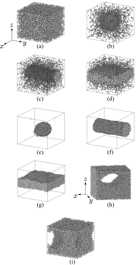
Figure 3: (Color online) Steady patterns made of the particles under the plane shear: (a) uniformly sheared phase, (b) coexistence of a spherical-droplet and gas, (c) coexistence of a dense-cylinder and gas, (d) coexistence of a dense-plate and gases, (e) an isolated spherical-droplet, (f) an isolated dense-cylinder, (g) an isolated dense-plate, (h) an inverse cylinder, and (i) an inverse droplet, where the corresponding dimensionless parameters $n^{\ast}$, $\dot{\gamma}^{\ast}$, and $\zeta^{\ast}$ for (a)–(i) are listed in Table 1. We note that gas particles in (b), (c) and (d) are drawn smaller than the real size for visibility.

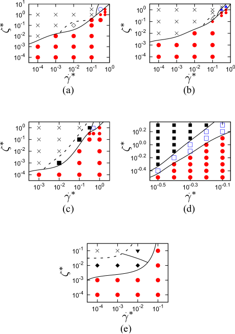
Figure 4: (Color online) Phase diagrams for various densities, where the dimensionless densities are given by (a) $n^{*}=0.0463$, (b) $0.156$, (c) $0.305$, (d) $0.305$ for $10^{-0.5}\leq\dot{\gamma}^{*}\leq 10^{-0.1}$, and (e) $0.723$, respectively. The spatial patterns corresponding to Fig. 3(a)–(i) are represented by red filled circles (Fig. 3(a)), blue open circles (Fig. 3(b)), blue filled upper triangles (Fig. 3(c)), blue open squares (Fig. 3(d)), black open diamond (Fig. 3(e)), black open upper triangles (Fig. 3(f)), black filled squares (Fig. 3(g)), black filled lower triangles (Fig. 3(h)), and black filled triangles (Fig. 3(i)), respectively. The steady states represented by the cross marks show various patterns depending on the initial velocities of particles.

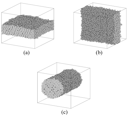
Figure 5: (Color online) Typical examples of initial configuration dependence when we start from the identical parameters ($n^{*}=0.305$, $\dot{\gamma}^{*}=10^{-3}$, $\zeta^{*}=10^{-2}$): (a) a dense-plate cluster parallel to $xy$ plane, (b) a dense-plate cluster parallel to $yz$ plane and (c) a dense-cylinder cluster parallel to $x$-axis.

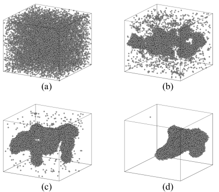
Figure 6: (Color online) Time evolution of configurations for $n^{*}=0.0904$, $\dot{\gamma}^{*}=10^{-1}$, $\zeta^{*}=10^{0.5}$. (a) $t^{*}=0$, (b) $50$, (c) $100$, and (d) $550$.

Figure 3 displays typical patterns formed by the particles in their steady states, which are characterized by the dimensionless parameters $n^{*}$, $\dot{\gamma}^{\ast}$, and $\zeta^{\ast}$ as listed in Table 1. Figure 4 shows phase diagrams in the steady states for (a) $n^{\ast}=0.0904$, (b) $0.156$, (c) $0.305$, and (d) $0.723$. Three of these phases, Figs. 3(a), (d) and (g), are similar to those observed in a quasi two-dimensional case with Sllod dynamics Takada2013 . If the shear is dominant, the system remains in a uniformly sheared phase (Fig. 3(a)). However, if the viscous heating by the shear is comparable with the energy dissipation, we find that a spherical-droplet, a dense-cylinder, and a dense-plate coexist for extremely dilute ($n^{\ast}=0.0904$), dilute ($n^{\ast}=0.156$), and moderately dense ($n^{\ast}=0.305$) gases, respectively (Figs. 3(b)–(d)). These three coexistence phases are realized by the competition between the equilibrium phase transition and the dynamic instability caused by inelastic collisions. Furthermore, if the energy dissipation is dominant, there are no gas particles in steady states (Figs. 3(e)–(g)). For an extremely high density case ($n^{\ast}=0.723$), we observe an inverse-cylinder, where the vacancy forms a “hole” passing through the dense region along the $y$-axis (Fig. 3(h)), and an inverse-droplet, where the shape of the vacancy is spherical (Fig. 3(i)). In our simulation, the role of particles in a dilute system corresponds to that of vacancies in a dense system. Thus, the system has a quasi particle-hole symmetry.
 Moreover, the shape of clusters depends on the initial condition of velocities of particles, even though a set of parameters such as the density, the shear rate, the dissipation rate and the variance of the initial velocity distribution function are identical when the dissipation is strong. We observe a dense-plate parallel to $xy$ plane (Fig. 5(a)), a dense-plate parallel to $yz$ plane (Fig. 5(b)), and a dense-cylinder parallel to $y$-axis (Fig. 5(c)) under the identical set of parameters. This initial velocity dependence appears in the region far from the coexistence phases, where the system evolves from aggregates of many clusters (see Fig. 6).

III.2 Velocity distribution function

We also measure the velocity distribution function (VDF) $P(u_{i})$ ($i=x,y,z$), where $u_{i}$ is the velocity fluctuation around the mean velocity field, $\bar{v}_{i}$, averaged over the time and different samples in the steady state. For simplicity, we focus only on the following three phases; the uniformly sheared phase (Fig. 3(a)), the dense-plate coexistence phase (Fig. 3(d)), and the dense-plate cluster phase (Fig. 3(g)). In this paper, we use the width $\Delta z=\sigma$ for bins in $z$-direction, while the bin sizes in both $x$ and $y$-directions are $L$ to evaluate VDF from our MD as in Fig. 7. It is remarkable that the VDF is almost isotropic Gaussians for the phases corresponding to Figs. 3(a) and (g) as well as deep inside of both the dense and the gas regions in the coexistence phase in Fig. 3(d) (see Figs. 8(a)–(d)). This is because we are interested in weak shear and weak dissipation cases without the influence of gravity. On the other hand, VDF is nearly equal to an anisotropic exponential function Vijayakumar2007 ; Alam2010 in the vicinity of the interface between the dense and the gas regions in the coexistence phase corresponding to Fig. 3(d) as in Figs. 8(e)–(g).

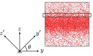
Figure 7: (Color online) A snapshot of our simulation for the plate-gases coexistence phase. Solid lines refer to the edges of a bin. The binwise velocity distribution function is calculated in each bin, whose width is $\Delta z=\sigma$. In addition, we introduce a new coordinate $(y^{\prime},z^{\prime})$, and $\theta$, which is the angle between $y^{\prime}$ and $y$-direction (in the counterclockwise direction) for later analysis.

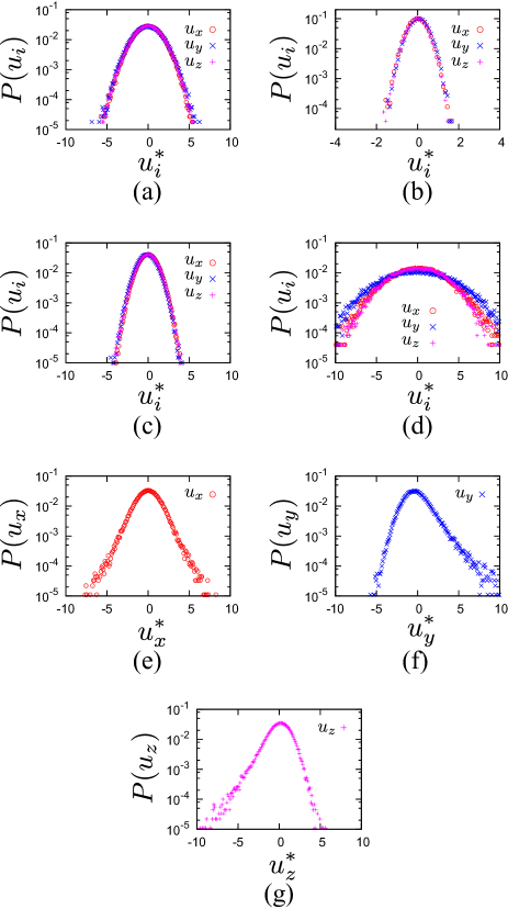
Figure 8: (Color online) Velocity distribution functions for various phases: (a) VDFs in the phase Fig. 3(a), (b) VDFs in the phase Fig. 3(g), (c) VDFs in the dense region of the phase Fig. 3(d), (d) VDFs in the dilute region of the phase Fig. 3(d), (e) VDF of $x$-direction in the interface of the phase Fig. 3(d), (f) VDF of $y$-direction in the interface of the phase Fig. 3(d), and (g) VDF of $z$-direction in the interface of the phase Fig. 3(d).

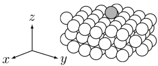
Figure 9: A schematic picture of the configuration of a gas particle (gray) and particles in the dense region (white). We assume that the wall particles are composed in a face-centered cubic lattice. We calculate the interaction energy between the gas particle and the wall particles whose distance is less than the cut-off length.

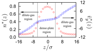
Figure 10: (Color online) The density and velocity profiles (in the $y$-direction) in the plate-gases coexistence phase ($n^{*}=0.305$, $\dot{\gamma}^{*}=10^{-0.2}$, $\zeta^{*}=10^{0.2}$), where $\bar{v}^{*}_{y}(z)=\bar{v}_{y}(z)\sqrt{m/\sigma\varepsilon}$.

We now explain the non-Gaussian feature near the interface by a simple stochastic model of a tracer particle subjected to Coulombic friction (the justification to use such a model is explained in Appendix B). Let us consider a situation that a gas particle hits and slides on the wall formed by the particles in the dense region (see Fig. 9). Because the velocity gradient in the gas region is almost constant as shown in Fig. 10, we may assume that a tracer particle in the gas near the interface is affected by a plane shear. Moreover, the tracer particle on a dense region may be influenced by Coulombic friction (see Appendix B). When we assume that the collisional force among gas particles can be written as the Gaussian random noise $\xi$, the equations of motion of a tracer particle at the position $\bm{r}$ may be given by

$$\frac{d\bm{r}}{dt} =\frac{\bm{p}}{m}+\dot{\gamma}z\hat{\rm{e}}_{y},$$ (4)

$$\frac{d\bm{p}}{dt} =-\mu F_{0}\frac{\bm{p}}{|\bm{p}|}-\dot{\gamma}p_{z}\hat{\bm{e}}_{y}+\bm{\xi},$$ (5)

where $\bm{p}$ is a peculiar momentum, which is defined by Eq. (4). Here we have introduced the friction constant $\mu_{0}$ and the effective force $F_{0}$ which is a function of the activation energy $\Delta E$ from the most stable trapped configuration of the solid crystal (see Fig. 9). Here, $\xi$ is assumed to satisfy

$$\left<\xi_{\alpha}(t)\right>=0,\quad\left<\xi_{\alpha}(t)\xi_{\beta}(t^{\prime})\right>=2D\delta_{\alpha,\beta}\delta(t-t^{\prime}),$$ (6)

where $\left<\cdots\right>$ is the average over the distribution of the random variable $\bm{\xi}$. $D$ is the diffusion coefficient in the momentum space, which satisfies the fluctuation-dissipation relation $D=\mu F_{0}\sqrt{mT/(d+1)}$ in the $d$-dimensional system with a temperature $T$. A set of Langevin equations (4) and (5) can be converted into the Kramers equation Kubo1991 ; Zwanzig2001 ; Kawarada2004 ; deGennes2005 ; Hayakawa2005 :

$$\frac{\partial f}{\partial t}= \left\{-\frac{\partial}{\partial\bm{r}}\cdot\left(\frac{\bm{p}}{m}+\dot{\gamma}z\hat{\bm{e}}_{y}\right)\right.$$

$$\left.+\frac{\partial}{\partial\bm{p}}\cdot\left(\dot{\gamma}p_{z}\hat{\bm{e}}_{y}+\mu F_{0}\frac{\bm{p}}{|\bm{p}|}+D\frac{\partial}{\partial\bm{p}}\right)\right\}f,$$ (7)

where $f=f(\bm{r},\bm{p},t)$ is the probability distribution function of the tracer particle.
 If we multiply Eq. (7) by $p^{2}$ and integrate over $\bm{p}$, we immediately obtain

$$\frac{\partial}{\partial t}\left<p^{2}\right>= -\frac{\partial}{\partial\bm{r}}\cdot\frac{\left<p^{2}\bm{p}\right>}{m}-\dot{\gamma}z\frac{\partial}{\partial y}\left<p^{2}\right>$$

$$-2\dot{\gamma}\left<p_{y}p_{z}\right>-2\mu F_{0}\left<p\right>+2D,$$ (8)

where $p=(p_{y}^{2}+p_{z}^{2})^{1/2}$. Because the third term on the right hand side (RHS) of Eq. (8) represents the viscous heating which is always positive as shown in Eq. (34) and the fourth term is the loss of the energy due to friction, the balance among the third, the fourth and the fifth terms on RHS of Eq. (8) produces a steady state. It should be noted that the first and the second terms on RHS do not contribute to the energy balance equation for the whole system.
 Here, we only consider the steady distribution, i.e. $\partial f/\partial t=0$. Thus, Eq. (7) is reduced to

$$\frac{\bm{p}}{m}\cdot \bm{\nabla}f+\dot{\gamma}z\frac{\partial}{\partial y}f-\dot{\gamma}p_{z}\frac{\partial}{\partial p_{y}}f$$

$$-\mu F_{0}\frac{\partial}{\partial\bm{p}}\cdot\left(\frac{\bm{p}}{|\bm{p}|}f\right)-D\Delta_{\bm{p}}f=0,$$ (9)

where $\Delta_{\bm{p}}=\partial^{2}/\partial p_{y}^{2}+\partial^{2}/\partial p_{z}^{2}$. If there is neither a shear nor a density gradient, we find that Eq. (9) has the steady solution obeying an exponential distribution, i.e. $f(\bm{p})=(\kappa^{2}/2\pi)\exp[-\kappa p]$, where we have introduced $\kappa\equiv\mu F_{0}/D$. We adopt the perturbative expression for $f$ in terms of $\epsilon\equiv\sigma/\lambda$, which is the ratio of the diameter $\sigma$ to the interface width $\lambda$, and the dimensionless shear rate $\dot{\gamma}^{\ast}$ as (see the derivation in Appendix D)

$$f(p,\theta) =f^{(0,0)}(p,\theta)+\epsilon f^{(0,1)}(p,\theta)+\dot{\gamma}^{\ast}f^{(1,0)}(p,\theta).$$ (10)

We also adopt the expansions

$$f^{(i,j)}(p,\theta)=\sum_{n=1}^{\infty}f_{n}^{(i,j)}\sin(n\theta),$$ (11)

with $(i,j)=(0,1)$ and $(1,0)$, where $\theta$ is the angle between $\bm{p}$ and $y$-axis (in the counterclockwise direction, see Fig. 7). Then, we can solve Eq. (9) perturbatively as

$$f(p,\theta) =f^{(0,0)}(p)+\epsilon f_{1}^{(0,1)}(p)\sin\theta+\dot{\gamma}^{\ast}f_{2}^{(1,0)}(p)\sin 2\theta,$$ (12)

where $f^{(0,0)}$, $f_{1}^{(0,1)}$ and $f_{2}^{(1,0)}$ are, respectively, given by

$$f^{(0,0)}(p) =\frac{\kappa^{2}}{2\pi}\exp\left(-\kappa p\right),$$ (13)

$$f_{1}^{(0,1)}(p) =-\frac{A}{6\pi\kappa}p\left(3+\kappa p+\kappa^{2}p^{2}\right)\exp\left(-\kappa p\right),$$ (14)

$$f_{2}^{(1,0)}(p) =-\frac{\kappa^{2}}{8\pi Dt_{0}}p^{2}\exp\left(-\kappa p\right).$$ (15)

Here, we have introduced $t_{0}=(m\sigma^{2}/\varepsilon)^{1/2}$ and $A$ given by Eq. (44). It should be noted that the other terms except for those in Eqs. (12)–(15) automatically disappear within the linear approximation as in Eq. (10).
 The second, the third and the fourth moments in $y^{\prime}$ and $z^{\prime}$-directions after the rotation by the angle of $\theta$ in the counterclockwise direction are, respectively, given by

$$\left<p_{y^{\prime},z^{\prime}}^{2}\right> =\frac{3}{\kappa^{2}}\left(1\mp\frac{5\dot{\gamma}}{2D\kappa^{2}}\sin 2(\theta-\psi)\right),$$ (16)

$$\left<p_{y^{\prime}}^{3}\right> =-\frac{765\epsilon A}{\kappa^{6}}\sin(\theta-\psi),$$ (17)

$$\left<p_{z^{\prime}}^{3}\right> =-\frac{765\epsilon A}{\kappa^{6}}\cos(\theta-\psi),$$ (18)

$$\left<p_{y^{\prime},z^{\prime}}^{4}\right> =\frac{45}{\kappa^{4}}\left(1\mp\frac{7\dot{\gamma}}{D\kappa^{2}}\sin 2(\theta-\psi)\right),$$ (19)

as shown in Appendix E, where $\left<p_{y^{\prime},z^{\prime}}^{n}\right>$ with $n=2$ or $4$ represents $\left<p_{y^{\prime}}^{n}\right>$ for a minus sign and $\left<p_{z^{\prime}}^{n}\right>$ for a plus sign, respectively. To reproduce the node of the third moment in MD, we phenomenologically introduce the angle $\psi$ and replace $\theta$ by $\theta-\psi$ in Eqs. (16)–(19). Here, we choose $\psi=2\pi/9$ to fit the node position of the third moment. We have not identified the reason why the direction of the node is deviated from the direction at which VDF becomes isotropic.
 Now, let us compare Eqs. (16)–(19) with MD for a set of parameters $(n^{\ast},\dot{\gamma}^{\ast},\zeta^{\ast})=(0.305,10^{-0.2},10^{0.2})$. From the density profile (Fig. 10) and the fitting to the second moment and the amplitude of the third moment, we obtain $\epsilon\simeq 0.20$, $\mu\simeq 1.3/\sqrt{m\varepsilon}$, $D=5.2\sqrt{m\varepsilon^{3}}/\sigma$, and $A\simeq 0.088/m^{2}\varepsilon^{2}$. It is surprised that Eqs. (16)–(19) can approximately reproduce the simulation results as in Fig. 11 except for the node positions of the second and the fourth moments.

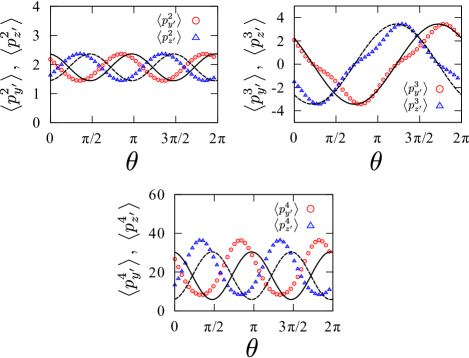
Figure 11: (Color online) The second, the third and the fourth moments obtained by MD for $\rho^{\ast}=0.305$, $\dot{\gamma}^{\ast}=10^{-0.2}$, $\zeta^{\ast}=10^{0.2}$ (circle: $y^{\prime}$-direction, upper triangle: $z^{\prime}$-direction) and those obtained by Eqs. (16)–(19) (solid line: $y^{\prime}$-direction, dashed line: $z^{\prime}$-direction).

For the explicit form of VDF, at first, we convert $f(p,\theta)$ to $f(p_{y},p_{z})$ as in Appendix F:

$$f(p_{y},p_{z})= \frac{\kappa^{2}}{2\pi}\exp\left(-\kappa p\right)\left[1+\frac{\epsilon A}{3\kappa^{3}}\left(3+\kappa p+\kappa^{2}p^{2}\right)\right.$$

$$\left.\times(p_{y}\sin\psi-p_{z}\cos\psi)\right.$$

$$\left.+\frac{\dot{\gamma}}{4D}\left\{(p_{y}^{2}-p_{z}^{2})\sin 2\psi-2p_{y}p_{z}\cos 2\psi\right\}\right].$$ (20)

We obtain the peculiar velocity distribution function in each direction by integrating Eq. (20) with respect to $u_{z}$ or $u_{y}$ as

$$P(u_{y})= \frac{m\kappa^{2}}{2\pi}\int_{-\infty}^{\infty}du_{z}\exp\left(-m\kappa u\right)$$

$$\times\left[1+\frac{m\epsilon A}{3\kappa^{3}}\left(3+m\kappa u+m^{2}\kappa^{2}u^{2}\right)u_{y}\sin\psi\right.$$

$$\left.+\frac{m^{2}\dot{\gamma}}{4D}(u_{y}^{2}-u_{z}^{2})\sin 2\psi\right],$$ (21)

$$P(u_{z})= \frac{m\kappa^{2}}{2\pi}\int_{-\infty}^{\infty}du_{y}\exp\left(-m\kappa u\right)$$

$$\times\left[1-\frac{m\epsilon A}{3\kappa^{3}}\left(3+m\kappa u+m^{2}\kappa^{2}u^{2}\right)u_{z}\cos\psi\right.$$

$$\left.+\frac{m^{2}\dot{\gamma}}{4D}(u_{y}^{2}-u_{z}^{2})\sin 2\psi\right],$$ (22)

where $u=(u_{y}^{2}+u_{z}^{2})^{1/2}$. These expressions semi-quantitatively reproduce VDF observed in our MD as in Fig. 12.

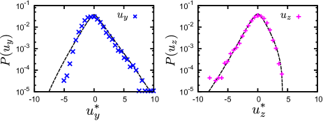
Figure 12: (Color online) VDFs in $y$-direction (left, cross) and $z$-direction (right, cross) obtained by our MD. The dashed lines in the left and right figures are the results of Eqs. (21) and (22), respectively.

IV discussion and conclusion

IV.1 Discussion

Let us discuss our results. In Sec. III.1, we do not discuss the time evolution of the granular temperature $T_{\rm g}=(m/3N)\sum_{i=1}^{N}|\bm{v}_{i}-\bm{V}|^{2}$, where $\bm{V}=\bm{V}(\bm{r},t)$ is the ensemble average velocity field Goldhirsch2003 ; Goldhirsch2008 . The granular temperature abruptly decreases to zero in the cluster phases Fig. 3(e)–(i) when a big cluster which absorbs all gas particles appears Takada2013_2 . To clarify the mechanism of abrupt change of the temperature during clusterings, we will need to study the more detailed dynamics.
 Moreover, to discuss the phase boundary between the uniformly sheared phase and the coexistence phases, we may use the stability analysis of a set of the hydrodynamic equations coupled with the phase transition dynamics Onuki2002 . Once we establish the set of hydrodynamic equations, it is straightforward to perform weakly nonlinear analysis for this system Saitoh2011 ; Alam2013 ; Shukla2013 . It should be noted that the set of equations may be only available near the phase boundary between the uniformly sheared phase and the coexistence phases.
 In Fig. 8, the VDF in a uniformly sheared phase is almost Gaussian. This result seems to be inconsistent with the results for ordinary gases under a uniform shear flow Garzo2003 , which showed that the VDF differs from Gaussian even in a uniformly sheared phase. In this study, however, we only restrict our interest to small inelastic and weakly sheared cases. This situation validates small deviation from Gaussian.

IV.2 Conclusion

We studied cohesive fine powders under a plane shear by controlling the density, the dimensionless shear rate and the dissipation rate. Depending on these parameters, we found the existence of various distinct steady phases as in Fig. 3, and we have drawn the phase diagrams for several densities as in Fig. 4. In addition, the shape of clusters depends on the initial condition of velocities of particles as in Fig. 5, when the dissipation is strong. We also found that there is a quasi particle-hole symmetry for the shape of clusters in steady states with respect to the density.
 We found that the velocity distribution functions near the interface between the dense region and the gas-like dilute region in the dense-plate coexistence phase deviate from the Gaussian as in Fig. 8. Introducing a stochastic model and its corresponding the Kramers equation (7), we obtain its perturbative VDFs as in Eqs. (21) and (22), which reproduce the semi-quantitative behavior of VDF observed in MD as in Fig. 12. This result suggests that the motion of a gas particle near the interface is subjected to Coulombic friction force whose origin is the activation energy in the dense region.

Appendix A Results of the physical boundary condition

In this Appendix, we present the results of our simulations under the flat boundary condition which is one of the typical physical boundaries to clarify the influence of the boundary condition. We prepare flat walls at $z=\pm L/2$, moving at velocities $\pm\dot{\gamma}L/2$ in $y$-direction, respectively. When a particle with a velocity $(v_{x},v_{y},v_{z})$ hits the walls at $z=\pm L/2$, the velocity is changed as $(v_{x},\pm\dot{\gamma}L/2-v_{y},-v_{z})$ after the collision, respectively. The phase diagram of the system for the physical boundary for $n^{*}=0.305$ is presented in Fig. 13. We have obtained three steady phases such as the uniformly sheared phase, the coexistence phase between dense-plate and gas regions, and the dense-plate cluster phase. The phase diagram is almost same as the corresponding one under the Lees-Edwards boundary condition (see Figs. 4(d)). This can be understood as follows: if two particles at the symmetric positions with respect to the origin of the system simultaneously collide the walls at $z=L/2$ and $-L/2$, the pair of velocities after collisions is same as that after passing across the boundaries at $z=\pm L/2$ for the system under the Lees-Edwards boundary condition. This is realized after the averaging over the collisions. Thus, the flat boundary condition is essentially equivalent to the Lees-Edwards boundary condition.

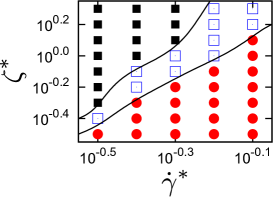
Figure 13: (Color online) Phase diagram under the flat boundary condition for $n^{*}=0.305$, uniformly sheared state (red filled circle, Fig. 3(a)), coexistence of a dense-plate and gases (blue open square, Fig. 3(d)), and an isolated dense-plate (black filled square, Fig. 3(g)).

Appendix B Calculation of Coulombic friction constant

In this appendix, we try to illustrate the existence of Coulombic friction force for the motion of a tracer particle near the interface. Let us consider a situation that a gas particle hits and slides on the wall formed by the particles in the dense region (see Fig. 9). If the kinetic energy of the gas particle is less than the potential energy formed by the particles in the dense region, it should be trapped in the potential well. Therefore, the motion of the gas particle is restricted near the interface. In this case, we can write the $N$-body distribution function near the interface $\rho(\bm{\Gamma},t)$ by using the distribution function in the equilibrium system as Evans2008 ; Chong2010_1 ; Chong2010_2 ; Hayakawa2013

$$\rho(\bm{\Gamma},t)=\rho_{\rm eq}(\bm{\Gamma})\exp\left[\int_{0}^{t}d\tau\Omega(-\tau,\bm{\Gamma},\dot{\gamma}_{l},\zeta)\right],$$ (23)

where $\bm{\Gamma}=\{\bm{r}_{i},\bm{p}_{i}\}_{i=1}^{N}$, $\rho_{\rm eq}(\bm{\Gamma})$ is the equilibrium distribution function at time $t=0$, and

$$\Omega(t,\bm{\Gamma},\dot{\gamma},\zeta)= -\beta\dot{\gamma}V\sigma_{yz}(t,\bm{\Gamma},\dot{\gamma},\zeta)$$

$$-2\beta{\cal R}(t,\bm{\Gamma},\dot{\gamma},\zeta)-\Lambda(t,\bm{\Gamma},\dot{\gamma},\zeta),$$ (24)

with

$$\sigma_{\alpha\beta}(t,\bm{\Gamma},\dot{\gamma},\zeta)= \sum_{i}\left\{\frac{p_{i,\alpha}p_{i,\beta}}{m}-\sum_{j\neq i}r_{i,\alpha}\frac{\partial U^{\rm LJ}(r_{ij})}{\partial r_{i,\beta}}\right.$$

$$\left.+\sum_{j\neq i}r_{i,\alpha}F_{\beta}^{\rm vis}(\bm{r}_{ij},\bm{v}_{ij})\right\},$$ (25)

$${\cal R}(t,\bm{\Gamma},\dot{\gamma},\zeta)= \frac{\zeta}{4}\sum_{i\neq j}\Theta(\sigma-r_{ij})(\bm{v}_{ij}\cdot\hat{\bm{r}}_{ij})^{2},$$ (26)

$$\Lambda(t,\bm{\Gamma},\dot{\gamma},\zeta)= -\frac{\zeta}{m}\sum_{i\neq j}\Theta(\sigma-r_{ij}),$$ (27)

$$F_{\beta}^{\rm vis}(\bm{r}_{ij},\bm{v}_{ij})= -\zeta\Theta(\sigma-r_{ij})(\bm{v}_{ij}\cdot\hat{\bm{r}}_{ij})\frac{r_{ij,\beta}}{r_{ij}}.$$ (28)

Here, we have introduced the inverse granular temperature $\beta=1/T$ and the local shear rate $\dot{\gamma}_{l}$ in the interface region. If the dissipation is small and the shear rate is not large, we may assume that $\Omega(-t)\simeq-\beta\dot{\gamma}V\sigma_{yz}^{\rm mf}(-t)$, where $\sigma_{yz}^{\rm mf}$ is the mean field $yz$ component of the stress tensor. We also assume that the stress tensor decays exponentially as $\sigma_{yz}^{\rm mf}(-t)\simeq\sigma_{yz}^{\rm mf}(0)\exp(-|t|/\tau_{0})$ Evans2008 , where $\tau_{0}$ is the relaxation time of the stress tensor. From these relationships, we may use the approximate expression

$$\rho(\bm{\Gamma},t)\simeq \prod_{i=1}^{N_{l}}\frac{1}{Z^{\rm mf}}\exp\left[-\beta\left(H^{\rm mf}-\Delta E_{i}\right)\right]$$

$$\times\exp\left(-\beta\tau_{0}\dot{\gamma}_{l}V_{l}\sigma_{yz}^{\rm mf}(0)\right),$$ (29)

where $H^{\rm mf}$ and $\Delta E_{i}$, are respectively, the mean field Hamiltonian per particle in the interface and the energy fluctuation of the particle $i$ which may be the activation energy from the local trap. Here $N_{l}$ and $V_{l}$ are, respectively, the number of particles and the volume in the interface region and $Z^{\rm mf}=\int d\bm{r}d\bm{p}\exp(-\beta H^{\rm mf})$. There are two characteristic time scales $\dot{\gamma}^{-1}$ and $\dot{\gamma}_{l}^{-1}$ corresponding to the uniform region and the interface between dense and dilute regions. Because the time scale is obtained from the average over the distribution function (29) or the local mean field distribution, the relationship between $\dot{\gamma}^{-1}$ and $\dot{\gamma}_{l}^{-1}$ is expected to be

$$\dot{\gamma}_{l}^{-1}=\dot{\gamma}^{-1}\exp\left[\beta(\Delta E-\tau_{0}\dot{\gamma}_{l}V_{l}\sigma_{yz}^{\rm mf}(0))\right],$$ (30)

where we have eliminated the suffix $i$ for the particle. This equation can be rewritten as

$$\sigma_{yz}^{\rm mf}(0)=\frac{1}{\tau_{0}\dot{\gamma}_{l}V_{l}}\left(\Delta E+T\ln\frac{\dot{\gamma}_{l}}{\dot{\gamma}}\right).$$ (31)

Therefore, we may estimate Coulombic friction constant as

$$\mu =\frac{\sigma_{yz}^{\rm mf}(0)}{P}=\frac{1}{\tau_{0}\dot{\gamma}_{l}PV_{l}}\left(\Delta E+T\ln\frac{\dot{\gamma}_{l}}{\dot{\gamma}}\right),$$ (32)

where $P\simeq 0.90\varepsilon/\sigma^{3}$, $V_{l}\simeq 4.3\sigma^{3}$, $\Delta E\simeq 3.5\varepsilon$ and $\dot{\gamma}_{l}\simeq 0.83(\varepsilon/m\sigma^{2})^{1/2}$ at the interface for a set of parameters $(n^{\ast},\dot{\gamma}^{\ast},\zeta^{\ast})=(0.305,10^{-0.2},10^{0.2})$. In this expression, we cannot determine the relaxation time $\tau_{0}$ from the simulation, which is estimated to reproduce the average value of the second moment with the aid of Eq. (16).

Appendix C Detailed calculation of the viscous heating term

In this appendix, let us calculate the average of the viscous heating term by using the distribution function near the interface. From Eq. (29), we can rewrite the distribution function with the aid of Eq. (25) as

$$\rho(\bm{\Gamma},t)\approx\frac{1}{Z}\prod_{i=1}^{N_{l}}\exp\left[-\beta\left(\frac{\bm{p}_{i}^{2}}{2m}+\tau_{0}\dot{\gamma}_{l}V_{l}\frac{p_{i,y}p_{i,z}}{m}\right)\right],$$ (33)

where $Z=\int\prod_{i=1}^{N_{l}}d\bm{r}_{i}d\bm{p}_{i}\exp[-\beta(\bm{p}_{i}^{2}/2m+\tau_{0}\dot{\gamma}_{l}V_{l}p_{i,y}p_{i,z}/m)]$. Then $\left<p_{y}p_{z}\right>$ is given by

$$\left<p_{y}p_{z}\right>= \int d\bm{\Gamma}p_{i,y}p_{i,z}\rho(\bm{\Gamma},t)$$

$$\propto \int_{-\infty}^{\infty}dp_{i,y}\int_{-\infty}^{\infty}dp_{i,z}p_{i,y}p_{i,z}$$

$$\times\exp\left[-\beta\left(\frac{\bm{p}_{i}^{2}}{2m}+\tau_{0}\dot{\gamma}_{l}V_{l}\frac{p_{i,y}p_{i,z}}{m}\right)\right]$$

$$= \int_{0}^{\infty}dp\int_{0}^{2\pi}d\theta p^{3}\sin\theta\cos\theta$$

$$\times\exp\left[-\beta\left(\frac{p^{2}}{2m}+\frac{\tau_{0}\dot{\gamma}_{l}V_{l}}{m}p^{2}\sin\theta\cos\theta\right)\right]$$

$$= -\frac{\pi}{2}\int_{0}^{\infty}dpp^{3}\exp\left(-\frac{\beta p^{2}}{2m}\right)I_{1}\left(\frac{\beta\tau_{0}\dot{\gamma}_{l}V_{l}}{2m}p^{2}\right),$$ (34)

where $I_{1}(x)$ is the modified Bessel function of the first kind Abramowitz1964 . Because $I_{1}(x)$ is positive for $x>0$, Eq. (34) ensures that the viscous heating term $-\dot{\gamma}\left<p_{y}p_{z}\right>$ is always positive near the interface.

Appendix D A perturbative solution of the Kramers equation

In this appendix, let us solve the Kramers equation (9) perturbatively to obtain the steady VDF. Later, we compare this solution with the result of MD.
 At first, we adopt the following three assumptions. The first assumption is that the distribution function is independent of both $x$ and $y$, the coordinates horizontal to the interface. We also assume that the distribution function $f$ depends on $z$, vertical to the interface, through the density and the granular temperature:

$$\frac{\partial f}{\partial z} =\frac{\partial f}{\partial n}\frac{dn}{dz}+\frac{\partial f}{\partial T}\frac{dT}{dz}.$$ (35)

Second, we assume that the changes of the density and the granular temperature near the interface can be characterized by the interface width $\lambda$ as

$$\frac{dn}{dz}\simeq-\frac{n_{0}}{\lambda},\quad\frac{dT}{dz}\simeq\frac{T_{0}}{\lambda},$$ (36)

where $n_{0}=n(z_{0})=(n_{l}+n_{g})/2$, $T_{0}=T(z_{0})=(T_{l}+T_{g})/2$. Here, $n_{l}$ and $T_{l}$ are the density and the granular temperature in the dense region, and $n_{g}$ and $T_{g}$ are those in the dilute region, respectively. Third, we also assume that the interface width $\lambda$ is much longer than the diameter of the particles $\sigma$, i.e. $\epsilon\equiv\sigma/\lambda\ll 1$. From these assumptions, $\partial f/\partial z$ may be rewritten as

$$\frac{\partial f}{\partial z} \simeq-\epsilon\left(\frac{n_{0}}{\sigma}\frac{\partial}{\partial n}-\frac{T_{0}}{\sigma}\frac{\partial}{\partial T}\right)f.$$ (37)

To solve Eq. (9), we adopt the perturbative expression Eq. (10). Equation (9), thus, reduces to the following three equations: for the zeroth order,

$$-\kappa\frac{\partial}{\partial\bm{p}}\cdot\left(\frac{\bm{p}}{|\bm{p}|}f^{(0,0)}\right)-\Delta_{\bm{p}}f^{(0,0)}=0,$$ (38)

for the first order of $\epsilon$,

$$-\frac{p_{z}}{mD} \left(\frac{n_{0}}{\sigma}\frac{\partial}{\partial n}-\frac{T_{0}}{\sigma}\frac{\partial}{\partial T}\right)f^{(0,0)}$$

$$-\kappa\frac{\partial}{\partial\bm{p}}\cdot\left(\frac{\bm{p}}{|\bm{p}|}f^{(0,1)}\right)-\Delta_{\bm{p}}f^{(0,1)}=0,$$ (39)

and for the first order of $\dot{\gamma}^{\ast}$,

$$-\frac{p_{z}}{D}\frac{\partial f^{(0,0)}}{\partial p_{y}}-\kappa\frac{\partial}{\partial\bm{p}}\cdot\left(\frac{\bm{p}}{|\bm{p}|}f^{(1,0)}\right)-\Delta_{\bm{p}}f^{(1,0)}=0.$$ (40)

The solution of Eq. (38) is given by

$$f^{(0,0)} =C_{1}\exp(-\kappa p)+C_{2}\exp(-\kappa p){\rm Ei}\left(\kappa p\right),$$ (41)

where ${\rm Ei}(x)$ is the exponential integral ${\rm Ei}(x)\equiv-\int_{-x}^{\infty}(e^{-t}/t)dt$ Abramowitz1964 , and $C_{1}$ and $C_{2}$ are the normalization constants. Here, we set $C_{2}=0$ because ${\rm Ei}(x)$ becomes infinite at $x=0$, and $C_{1}=\kappa^{2}/2\pi$ to satisfy the normalization condition without the shear and the density gradient. Using Eq. (41), Equations (39) and (40) can be represented in the polar coordinates as

$$A\left(p^{2}-\frac{2}{\lambda}p\right)f^{(0,0)}\sin\theta$$

$$=\kappa\left(\frac{1}{p}+\frac{\partial}{\partial p}\right)f^{(0,1)}+\left(\frac{\partial^{2}}{\partial p^{2}}+\frac{1}{p}\frac{\partial}{\partial p}+\frac{1}{p^{2}}\frac{\partial^{2}}{\partial\theta^{2}}\right)f^{(0,1)},$$ (42)

and

$$\frac{\kappa}{2Dt_{0}}pf^{(0,0)}\sin 2\theta$$

$$=\kappa\left(\frac{1}{p}+\frac{\partial}{\partial p}\right)f^{(1,0)}+\left(\frac{\partial^{2}}{\partial p^{2}}+\frac{1}{p}\frac{\partial}{\partial p}+\frac{1}{p^{2}}\frac{\partial^{2}}{\partial\theta^{2}}\right)f^{(1,0)},$$ (43)

where we have introduced $A$ as

$$A=\frac{n_{0}}{m\sigma D}\frac{\partial\kappa}{\partial n}-\frac{T_{0}}{m\sigma D}\frac{\partial\kappa}{\partial T}.$$ (44)

To solve Eqs. (42) and (43), we adopt the expansions for $f^{(i,j)}(p,\theta)=\sum_{n=1}^{\infty}f_{n}^{(i,j)}(p)\sin(n\theta)$ with $(i,j)=(0,1)$ and $(1,0)$ Hayakawa2005 . Equation (42) for each $n$ reduces to the following equations: for $n=1$,

$$\frac{A\kappa^{2}}{2\pi}\left(p^{2}-\frac{2}{\kappa}p\right)\exp(-\kappa p)$$

$$=\kappa\left(\frac{1}{p}+\frac{\partial}{\partial p}\right)f_{1}^{(0,1)}+\left(\frac{\partial^{2}}{\partial p^{2}}+\frac{1}{p}\frac{\partial}{\partial p}-\frac{1}{p^{2}}\right)f_{1}^{(0,1)},$$ (45)

and for $n\neq 1$,

$$0=\kappa\left(\frac{1}{p}+\frac{\partial}{\partial p}\right)f_{n}^{(0,1)}+\left(\frac{\partial^{2}}{\partial p^{2}}+\frac{1}{p}\frac{\partial}{\partial p}-\frac{n^{2}}{p^{2}}\right)f_{n}^{(0,1)}.$$ (46)

The solutions of Eqs. (45) and (46) are, respectively, given by

$$f_{1}^{(0,1)}= \frac{C_{11}}{p}+C_{12}\frac{1+\kappa p}{\kappa^{2}p}$$

$$-\frac{A}{6\pi}\frac{6+6\kappa p+3\kappa^{2}p^{2}+\kappa^{3}p^{3}+\kappa^{4}p^{4}}{\kappa^{3}p}\exp(-\kappa p),$$ (47)

and

$$f_{n}^{(0,1)}= C_{n1}(\kappa p)^{n}\exp(-\kappa p)U(n,2n+1,\kappa p)$$

$$+C_{n2}(\kappa p)^{n}\exp(-\kappa p)L_{-n}^{2n}(\kappa p),$$ (48)

for $n\neq 1$, where $U(a,b,x)$ and $L_{a}^{b}(x)$ are, respectively, the confluent hypergeometric function and Laguerre’s bi-polynomial Abramowitz1964 , and the normalization constants $C_{n1}$ and $C_{n2}$ ($n=1,2,\cdots$) will be determined later. Similarly, Equation (43) for each $n$ reduces to the following equations: for $n=2$,

$$\frac{\kappa^{3}}{4\pi Dt_{0}}p\exp(-\kappa p)$$

$$=\kappa\left(\frac{1}{p}+\frac{\partial}{\partial p}\right)f_{2}^{(1,0)}+\left(\frac{\partial^{2}}{\partial p^{2}}+\frac{1}{p}\frac{\partial}{\partial p}-\frac{4}{p^{2}}\right)f_{2}^{(1,0)},$$ (49)

and for $n\neq 2$,

$$0=\kappa\left(\frac{1}{p}+\frac{\partial}{\partial p}\right)f_{n}^{(1,0)}+\left(\frac{\partial^{2}}{\partial p^{2}}+\frac{1}{p}\frac{\partial}{\partial p}-\frac{n^{2}}{p^{2}}\right)f_{n}^{(1,0)}.$$ (50)

The solutions of Eqs. (49) and (50) are, respectively, given by

$$f_{2}^{(1,0)}= C_{23}\frac{3-\kappa p}{p^{2}}+C_{24}\frac{6+4\kappa p+\kappa^{2}p^{2}}{\kappa^{4}p^{2}}\exp(-\kappa p)$$

$$+\frac{1}{8\pi Dt_{0}}\frac{72+48\kappa p+12\kappa^{2}p^{2}-\kappa^{4}p^{4}}{\kappa^{2}p^{2}}\exp(-\kappa p),$$ (51)

and

$$f_{n}^{(1,0)}= C_{n3}(\kappa p)^{n}\exp(-\kappa p)U(n,2n+1,\kappa p)$$

$$+C_{n4}(\kappa p)^{n}\exp(-\kappa p)L_{-n}^{2n}(\kappa p),$$ (52)

for $n\neq 2$, where the normalization constants $C_{n3}$ and $C_{n4}$ ($n=1,2,\cdots$) will be determined later.
 Here, let us determine the normalization constants $C_{n1},\cdots,C_{n4}$ ($n=1,2,\cdots$). The distributions $f_{n}^{(0,1)}$ and $f_{n}^{(1,0)}$ should be finite at $p=0$ and approach zero for large $p$. Therefore, we obtain

$$C_{11}=0,\quad C_{12}=\frac{A}{\pi\kappa},\quad C_{23}=0,\quad C_{24}=-\frac{3\kappa^{2}}{2\pi Dt_{0}},$$

$$C_{n1}=0,\quad C_{n2}=0\quad(n\neq 1),$$

$$C_{n3}=0,\quad C_{n4}=0\quad(n\neq 2).$$ (53)

From these results, we obtain

$$f(p,\theta) =f^{(0,0)}+\epsilon f_{1}^{(0,1)}\sin\theta+\dot{\gamma}^{\ast}f_{2}^{(1,0)}\sin 2\theta,$$ (54)

where $f^{(0,0)}$, $f_{1}^{(0,1)}$ and $f_{2}^{(1,0)}$ are, respectively, given by

$$f^{(0,0)}(p) =\frac{\kappa^{2}}{2\pi}\exp(-\kappa p),$$ (55)

$$f_{1}^{(0,1)}(p) =-\frac{A}{6\pi\kappa}p(3+\kappa p+\kappa^{2}p^{2})\exp(-\kappa p),$$ (56)

$$f_{2}^{(1,0)}(p) =-\frac{\kappa^{2}}{8\pi Dt_{0}}p^{2}\exp(-\kappa p).$$ (57)

Appendix E Detailed calculations of various moments

In this appendix, we calculate the $n$-th moments of $p_{y^{\prime}}$ and $p_{z^{\prime}}$ using the distribution function obtained in Appendix D. From the definition of the moment, $n$-th moment of an arbitrary function $G(\bm{p})$ is given by

$$\left<G^{n}\right>=\int d\bm{p}\hskip 1.99997ptG^{n}(p,\varphi)f(p,\varphi).$$ (58)

We rotate the coordinate the coordinate $(y,z)$ by $\theta$ counterclockwise and introduce the new Cartesian coordinate $(y^{\prime},z^{\prime})$ as in Fig. 7. From this definition, we obtain the $n$-th moments of $p_{y^{\prime}}$, for $n=2$,

$$\left<p_{y^{\prime}}^{2}\right>= \int_{0}^{\infty}dp\int_{0}^{2\pi}d\varphi p^{3}\cos^{2}(\varphi-\theta)$$

$$\times\left[f^{(0,0)}(p)+\epsilon f_{1}^{(0,1)}(p)\sin\varphi+\dot{\gamma}^{\ast}f_{2}^{(1,0)}(p)\sin 2\varphi\right]$$

$$= \frac{3}{\kappa^{2}}\left(1-\frac{5\dot{\gamma}}{2D\kappa^{2}}\sin 2\theta\right),$$ (59)

for $n=3$,

$$\left<p_{y^{\prime}}^{3}\right>= \int_{0}^{\infty}dp\int_{0}^{2\pi}d\varphi p^{4}\cos^{3}(\varphi-\theta)$$

$$\times\left[f^{(0,0)}(p)+\epsilon f_{1}^{(0,1)}(p)\sin\varphi+\dot{\gamma}^{\ast}f_{2}^{(1,0)}(p)\sin 2\varphi\right]$$

$$= -\frac{765\epsilon A}{\kappa^{7}}\sin\theta,$$ (60)

and for $n=4$,

$$\left<p_{y^{\prime}}^{4}\right>= \int_{0}^{\infty}dp\int_{0}^{2\pi}d\varphi p^{5}\cos^{4}(\varphi-\theta)$$

$$\times\left[f^{(0,0)}(p)+\epsilon f_{1}^{(0,1)}(p)\sin\varphi+\dot{\gamma}^{\ast}f_{2}^{(1,0)}(p)\sin 2\varphi\right]$$

$$= \frac{45}{\kappa^{4}}\left(1-\frac{7\dot{\gamma}}{D\kappa^{2}}\sin 2\theta\right).$$ (61)

Similarly, we can calculate the each moment of $p_{z^{\prime}}$ so that we obtain Eqs. (16)–(19).

Appendix F Velocity distribution function for each direction

In this appendix, we derive the velocity distribution function in the Cartesian coordinate $(y,z)$ at first, and calculate the velocity distribution functions in $y$ and $z$-directions. The velocity distribution function in the polar coordinates $(p,\theta)$ is given by Eq. (12), where we replace $\theta$ by $\theta-\psi$ as in Eqs. (16)–(19), which can be converted into the form in Cartesian coordinate as

$$f(p_{y},p_{z})= \frac{\kappa^{2}}{2\pi}\exp(-\kappa p)\left[1-\frac{\epsilon A}{3\kappa^{3}}p(3+\kappa p+\kappa^{2}p^{2})\sin(\theta-\psi)-\frac{\dot{\gamma}}{4D}p^{2}\sin 2(\theta-\psi)\right]$$

$$= \frac{\kappa^{2}}{2\pi}\exp(-\kappa p)\left[1+\frac{\epsilon A}{3\kappa^{3}}(3+\kappa p+\kappa^{2}p^{2})(p_{y}\sin\psi-p_{z}\cos\psi)+\frac{\dot{\gamma}}{4D}\left\{(p_{y}^{2}-p_{z}^{2})\sin 2\psi-2p_{y}p_{z}\cos 2\psi\right\}\right],$$ (62)

where $p=\sqrt{p_{y}^{2}+p_{z}^{2}}$. Next, let us calculate the velocity distribution functions in $y$ and $z$ directions. In this paper, we focus on the VDF for the fluctuation velocity, which is defined by the deviation from the average velocity. Therefore, we can replace $p_{y}$ and $p_{z}$ by $mu_{y}$ and $mu_{z}$ in Eq. (62). The velocity distribution function in $y$-direction, $P(u_{y})$, is given by integrating Eq. (62) with respect to $u_{z}$ as

$$P(u_{y})= \int_{-\infty}^{\infty}d(mu_{z})f(mu_{y},mu_{z})$$

$$= \frac{m\kappa^{2}}{2\pi}\int_{-\infty}^{\infty}du_{z}\exp\left(-m\kappa u\right)\left[1+\frac{m\epsilon A}{3\kappa^{3}}\left(3+m\kappa u+m^{2}\kappa^{2}u^{2}\right)u_{y}\sin\psi+\frac{m^{2}\dot{\gamma}}{4D}(u_{y}^{2}-u_{z}^{2})\sin 2\psi\right],$$ (63)

where $u=\sqrt{u_{y}^{2}+u_{z}^{2}}$. Similarly, we can calculate the velocity distribution function in $z$-direction $P(p_{z})$ as

$$P(u_{z})= \int_{-\infty}^{\infty}d(mu_{y})f(mu_{y},mu_{z})$$

$$= \frac{m\kappa^{2}}{2\pi}\int_{-\infty}^{\infty}du_{y}\exp\left(-m\kappa u\right)\left[1-\frac{m\epsilon A}{3\kappa^{3}}\left(3+m\kappa u+m^{2}\kappa^{2}u^{2}\right)u_{z}\cos\psi+\frac{m^{2}\dot{\gamma}}{4D}(u_{y}^{2}-u_{z}^{2})\sin 2\psi\right].$$ (64)

References

- (1) H. Krupp, Adv. Colloid Interface Sci. 1, 111 (1967).
- (2) J. Visser, Powder Technol. 58, 1 (1989).
- (3) J. M. Valverde, A. Castellanos, A. Ramos, and P. K. Watson, Phys. Rev. E 62, 6851 (2000).
- (4) J. Tomas, Particul. Sci. Technol. 19, 95 (2001).
- (5) F. Cansell, C. Aymonier, and A. Loppinet-Serani, Curr. Opin. Solid St. M. 7, 31 (2003).
- (6) J. Tomas, Granul. Matter 6, 75 (2004).
- (7) A. Castellanos, Adv. Phys. 54, 263 (2005).
- (8) H.-J. Butt, B. Cappella, and M. Kappl, Surf. Sci. Rep. 59, 1 (2005).
- (9) J. Tomas, Chem. Eng. Sci. 62, 1997 (2007).
- (10) R. Tykhoniuk, J. Tomas, S. Luding, M. Kappl, L. Heim, and H.-J. Butt, Chem. Eng. Sci. 62, 2843 (2007).
- (11) G. Calvert, M. Ghadiri, and R. Tweedie, Adv. Powder Technol. 20, 4 (2009).
- (12) J. R. van Ommen, J. M. Valverde, and R. Pfeffer, J. Nanopart. Res. 14, 1 (2012).
- (13) J. N. Israelachvili, Intermolecular and Surface Forces Third Edition (Academic Press, New York, 2011).
- (14) K. L. Johnson, K. Kendall, and A. D. Roberts, Proc. R. Soc. Lond. A 324, 301 (1971).
- (15) B. V. Derjaguin, I. I. Abrikosova, and E. M. Lifshitz, Chem. Soc. Rev. 10, 295 (1956).
- (16) B. V. Derjaguin, V. M. Muller, and Y. P. Toporov, J. Colloid Interface Sci. 53, 314 (1975).
- (17) K. Z. Y. Yen and T. K. Chaki, J. Appl. Phys. 71, 3164 (1992).
- (18) C. Thornton, K. K. Yin, and M. J. Adams, J. Phys. D: Appl. Phys. 29, 424 (1996).
- (19) T. Mikami, H. Kamiya, and M. Horio, Chem. Eng. Sci. 53, 1927 (1998).
- (20) G. Bartels, T. Unger, D. Kadau, D. E. Wolf, and J. Kertész, Granul. Matter 7, 139 (2005).
- (21) S. Luding, R. Tukhoniuk, and J. Tomas, Chem. Eng. Technol. 26, 1229 (2003).
- (22) S. Luding, Powder Technol. 158, 45 (2005).
- (23) S. Luding, Granul. Matter 10, 235 (2008).
- (24) J. R. Royer, D. J. Evans, L. Oyarte, E. Kapit, M. Möbius, S. R. Waitukatis, and H. M. Jaeger, Nature (London), 459, 1110 (2009).
- (25) N. Kumar and S. Luding, arXiv:1407.6167.
- (26) S. Gonzalez, A. R. Thornton, and S. Luding, arXiv:1407.2370.
- (27) D. Hornbaker, R. Albert, I. Albert, A.-L. Barabási, and P. Schiffer, Nature 387, 765 (1997).
- (28) L. Bocquet, E. Charlaix, S. Ciliberto, and J. Crassous, Nature 396, 735 (1998).
- (29) C. D. Willett, M. J. Adams, S. A. Johnson, and J. P. K. Seville, Langmuir 16, 9396 (2000).
- (30) S. T. Nase, W. L. Vargas, A. A. Abatan, and J. J. MacCarthy, Powder Technol. 116, 214 (2001).
- (31) S. Herminghaus, Adv. Phys. 54, 221 (2005).
- (32) N. Mitarai and F. Nori, Adv. Phys. 55, 1 (2006).
- (33) S. Ulrich and A. Zippelius, Phys. Rev. Lett. 109, 166001 (2012).
- (34) F. Gerl and A. Zippelius, Phys. Rev. E 59, 2361 (1999).
- (35) H. Hayakawa and H. Kuninaka, Chem. Eng. Sci. 57, 239 (2002).
- (36) A. Awasthi, S. C. Hendy, P. Zoontjens, and S. A. Brown, Phys. Rev. Lett. 97, 186103 (2006).
- (37) N. V. Brilliantov, N. Albers, F. Spahn, and T. Pöschel, Phys. Rev. E 76, 051302 (2007).
- (38) M. Suri and T. Dumitrică, Phys. Rev. B 78, 081405 (2008).
- (39) H. Kuninaka and H. Hayakawa, Phys. Rev. E 79, 031309 (2009).
- (40) K. Saitoh, A. Bodrova, H. Hayakawa, and N. V. Brilliantov, Phys. Rev. Lett. 105, 238001 (2010).
- (41) H. Kuninaka and H. Hayakawa, Phys. Rev. E 86, 051302 (2012).
- (42) H. Tanaka, K. Wada, T. Suyama, and S. Okuzumi, Prog. Theor. Phys. Supp. 195, 101 (2012).
- (43) R. Murakami and H. Hayakawa, Phys. Rev. E 89, 012205 (2014).
- (44) J.-P. Hansen and L. Verlet, Phys. Rev. 184, 151 (1969).
- (45) J. J. Nicolas, K. E. Gubbins, W. B. Streett, and D. J. Tildersley, Mol. Phys. 37, 1429 (1979).
- (46) Y. Adachi, I. Fijihara, M. Takamiya, and K. Nakanishi, Fluid Phase Equilibr. 39, 1 (1988).
- (47) A. Lotfi, J. Vrabec, and J. Fischer, Mol. Phys. 76, 1319 (1992).
- (48) J. K. Johnson, J. A. Zollweg, and K. E. Gubbins, Mol. Phys. 78, 591 (1993).
- (49) J. Kolafa, H. L. Vörtler, K. Aim, and I. Nezbeda, Mol. Simulat. 11, 305 (1993).
- (50) R. H. Heist and H. He, J. Phys. Chem. Ref. Data 23, 781 (1994).
- (51) A. Laaksonen and D. Kashchiev, J. Chem. Phys. 98, 7748 (1994).
- (52) K. Yasuoka and M. Matsumoto, J. Chem. Phys. 109, 8451 (1998).
- (53) I. Goldhirsch and G. Zanetti, Phys. Rev. Lett. 70, 1619 (1993).
- (54) I. Goldhirsch, M.-L. Tan, and G. Zanetti, J. Sci. Comput. 8, 1 (1993).
- (55) S. McNamara and W. R. Young, Phys. Rev. E 53, 5089 (1996).
- (56) S. McNamara, Phys. Fluids A 5, 3056, (1993).
- (57) N. Brilliantov, C. Salueña, T. Schwager, and T. Pöschel, Phys. Rev. Lett. 93, 134301 (2004).
- (58) M. E. Lasinski, J. S. Curtis, and J. F. Pekny, Phys. Fluids 16, 265 (2004).
- (59) S. L. Conway and B. J. Glasser, Phys. Fluids 16, 509 (2004).
- (60) K. Saitoh and H. Hayakawa, Phys. Rev. E 75, 021302 (2007).
- (61) M. Alam and P. Shukla, J. Fluid Mech. 716, 349 (2013).
- (62) P. Shukla and M. Alam, J. Fluid Mech. 718, 131 (2013).
- (63) Y. Gu, S. Chialvo, and S. Sundaresan, Phys. Rev. E 90, 032206 (2014).
- (64) A. W. Lees and S. F. Edwards, J. Phys. C: Solid State Phys. 5, 1921 (1972).
- (65) S. Takada and H. Hayakawa, AIP Conf. Proc. 1542, 819 (2013).
- (66) D. J. Evans and G. P. Morriss, Phys. Rev. A 30, 1528 (1984).
- (67) D. J. Evans and G. Morriss, Statistical Mechanics of Nonequilibrium Liquids Second Edition (Cambridge University Press, Cambridge, 2008).
- (68) D. Chandler and J. D. Weeks, Phys. Rev. Lett. 25, 149 (1970).
- (69) J. D. Weeks, D. Chandler, and H. C. Andersen, J. Chem. Phys. 54, 5237 (1971).
- (70) S. Takada and H. Hayakawa, AIP Conf. Proc. 1518, 741 (2013).
- (71) K. C. Vijayakumar and M. Alam, Phys. Rev. E 75, 051306 (2007).
- (72) M. Alam and V. K. Chikkadi, J. Fluid Mech. 653, 175 (2010).
- (73) R. Kubo, M. Toda and N. Hashitsume, Statistical Physics II: Nonequilibrium Statistical Mechanics (Springer, Berlin, 1991).
- (74) R. Zwanzig, Nonequilibrium Statistical Mechanics (Oxford University Press, New York, 2001).
- (75) A. Kawarada and H. Hayakawa, J. Phys. Soc. Jpn. 73, 2037 (2004).
- (76) P.-G. de Gennes, J. Stat. phys. 119, 953 (2005).
- (77) H. Hayakawa, Physica D 205, 48 (2005).
- (78) I. Goldhirsch, Annu. Rev. Fluid Mech. 35, 267 (2003).
- (79) I. Goldhirsch, Powder Technol. 182, 130 (2008).
- (80) A. Onuki, Phase Transition Dynamics (Cambridge University Press, Cambridge, 2002).
- (81) K. Saitoh and H. Hayakawa, Granul. Matter 13, 697 (2011).
- (82) V. Garzó and A. Santos, Kinetic Theory of Gases in Shear Flows Nonlinear Transport (Kluwer Academic Publishers, Dordrecht, 2003).
- (83) S.-H. Chong, M. Otsuki, and H. Hayakawa, Prog. Theor. Phys. Suppl. 184, 72 (2010).
- (84) S.-H. Chong, M. Otsuki, and H. Hayakawa, Phys. Rev. E. 81, 041130 (2010).
- (85) H. Hayakawa and M. Otsuki, Phys. Rev. E 88, 032117 (2013).
- (86) M. Abramowitz and I. A. Stegun, Handbook of Mathematical Functions: With Formulas, Graphs, and Mathematical Tables (Dover Publications, New York, 1964).