On the Randić index and
conditional parameters of a graph

Abstract

The aim of this paper is to study some parameters of simple graphs related with the degree of the vertices. So, our main tool is the $n\times n$ matrix ${\cal A}$ whose ($i,j$)-entry is

$$a_{ij}=\left\{\begin{array}[]{ll}\frac{1}{\sqrt{\delta_{i}\delta_{j}}}&{\rm if}\quad v_{i}\sim v_{j};\\ 0&{\rm otherwise,}\end{array}\right.$$

where $\delta_{i}$ denotes the degree of the vertex $v_{i}$. We study the Randić index and some interesting particular cases of conditional excess, conditional Wiener index, and conditional diameter. In particular, using the matrix ${\cal A}$ or its eigenvalues, we obtain tight bounds on the studied parameters.

1 Introduction

In order to deduce properties of graphs from results and methods of algebra, firstly we need to translate properties of graphs into algebraic properties. In this sense, a natural way is to consider algebraic structures or algebraic objects as, for instance, groups or matrices. In particular, the use of matrices allows us to use methods of linear algebra to derive properties of graphs. There are various matrices that are naturally associated with graphs, such as the adjacency matrix, the Laplacian matrix, and the incidence matrix [1, 8, 3]. One of the main aims of algebraic graph theory is to determine how, or whether, properties of graphs are reflected in the algebraic properties of such matrices [8]. The aim of this paper is to study the Randić index and some interesting particular cases of conditional excess, conditional Wiener index, and conditional diameter. All these parameters are related with the degree of the vertices of the graph. So, our main tool will be a suitable adjacency matrix that we call degree-adjacency matrix.

The plan of the paper is the following: in Section 2 we emphasize some of the main properties of the degree-adjacency matrix. The remaining sections are devoted to study the relationship between the degree-adjacency matrix (or its eigenvalues) and several parameters of graphs. More precisely, in Section 3 we obtain bounds on the Randić index, in Section 4 we obtain bounds on a particular case of conditional excess, Section 5 is devoted to bound the degree diameter and, finally, in section 6 we obtain bounds on a particular case of conditional Wiener index.

We begin by stating some notation. In this paper all graphs $\Gamma=(V,E)$ will be finite, undirected and simple. We will assume that $|V|=n$ and $|E|=m$. The distance between vertices $u,v\in V(\Gamma)$ will be denoted by $\partial(u,v)$. The degree of a vertex $v_{i}\in V(\Gamma)$ will be denoted by $\delta(v_{i})$ (or by $\delta_{i}$ for short), the minimum degree of $\Gamma$ will be denoted by $\delta$ and the maximum by $\Delta$.

2 Degree-adjacency matrix

We define the degree-adjacency matrix of a graph $\Gamma$ of order $n$ as the $n\times n$ matrix ${\cal A}$ whose ($i,j$)-entry is

$$a_{ij}=\left\{\begin{array}[]{ll}\frac{1}{\sqrt{\delta_{i}\delta_{j}}}&{\rm if}\quad v_{i}\sim v_{j};\\ 0&{\rm otherwise.}\end{array}\right.$$

The matrix ${\cal A}$ can be regarded as the adjacency matrix of a weighted graph in which the edge-weight ${\emph{R}}(v_{i}v_{j})$ of the edge $v_{i}v_{j}$ is equal to ${\emph{R}}(v_{i}v_{j})=\frac{1}{\sqrt{\delta_{i}\delta_{j}}}$, thus justifying the terminology used. The weight ${\emph{R}}(v_{i}v_{j})$ will be called the Randić weight of the edge $v_{i}v_{j}\in E$. We will say that a graph is weight-regular if each of its edges has the same Randić weight. Particular cases of weight-regular graphs are the class of regular graphs and the class of semi-regular bipartite graphs.

If we consider the vector $\nu=(\sqrt{\delta_{1}},\sqrt{\delta_{2}},...,\sqrt{\delta_{n}})$, then we have ${\cal A}\nu=\nu$. Thus, $\lambda=1$ is an eigenvalue of ${\cal A}$ and $\nu$ is an eigenvector associated to $\lambda$. Hence, as ${\cal A}$ is non-negative and irreducible in the case of connected graphs, by the Perron-Frobenius theorem, $\lambda=1$ is a simple eigenvalue and $\lambda=1\geq|\lambda_{j}|$ for every eigenvalue $\lambda_{j}$ of ${\cal A}$. Therefore, we have

$$\|{\cal A}x\|\leq\|x\|,\quad\forall x\in\mathbb{R}^{n}.$$ (1)

Notice that the above inequality holds also in the case of non-connected graphs.

Hereafter the eigenvalues of ${\cal A}$ will be called degree-adjacency eigenvalues of $\Gamma$.

It is well-known that there are non-isomorphic graphs that have the same standard adjacency eigenvalues with the same multiplicities (the so called cospectral graphs). For instance, two connected graphs, both having the characteristic polynomial $P(x)=x^{6}-7x^{4}-4x^{3}+7x^{2}+4x-1$, are shown in Figure 1.

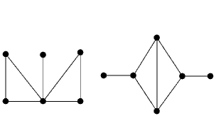
Figure 1: Two cospectral graphs but not cospectral with regard to ${\cal A}$

Therefore, we can try to study cospectral graphs by using an alternative matrix, for instance, the degree-adjacency matrix ${\cal A}$. If we consider the matrix ${\cal A}$, the eigenvalues of both graphs are different: the left hand side graph has degree-adjacency eigenvalues 1, $\pm\frac{1}{2}$ and $-\frac{1}{4}\left(1\pm\sqrt{2.6}\right)$ (where the eigenvalue $-\frac{1}{2}$ has multiplicity 2), on the other hand, the right hand side graph has degree-adjacency eigenvalues 1, $\frac{-1\pm\sqrt{2}}{3}$, $\pm\frac{\sqrt{3}}{3}$ and $-\frac{1}{3}$. Even so, the degree-adjacency eigenvalues do not determine the graph. That is, there are non-isomorphic graphs (and non-cospectral) that are cospectral with regard to the degree-adjacency matrix. For instance, the degree-adjacency eigenvalues of the cycle graph $C_{4}$ and the semi-regular bipartite graph $K_{1,3}$ are the same: $1,0,0,-1$. However, the standard eigenvalues are $2,0,0,-2$, in the case of $C_{4}$, and $\sqrt{3},0,0,-\sqrt{3}$ in the case of $K_{1,3}$.

It is easy to see that there are some classes of graphs in which the standard eigenvalues, $\vartheta_{1}\geq\vartheta_{2}\geq\cdots\geq\vartheta_{n}$, and the degree-adjacency eigenvalues, $\lambda_{1}\geq\lambda_{2}\geq\cdots\geq\lambda_{n}$, are directly related. For instance, in the case of weight-regular graphs, of weight $w^{-1}$, the adjacency matrix, ${\bf A}$, and the degree-adjacency matrix are related by ${\cal A}(\Gamma)=\frac{1}{w}{\bf A}(\Gamma)$. Thus, the eigenvalues of both matrices are related by

$$\lambda_{l}=\frac{\vartheta_{l}}{w},\quad l\in\{1,...,n\}.$$ (2)

As in the case of the adjacency matrix, there are some classes of graphs in which we can deduce a formula to compute the characteristic polynomial, $\Psi$, of the degree-adjacency matrix. For instance, from the degree-adjacency matrix of the path graph, $\Gamma=P_{n}$, we deduce that

$$\Psi({\cal A}(P_{n}),\lambda)=\lambda\Phi_{n}(\lambda)+\frac{1}{2}\Phi_{n-1}(\lambda),\quad n\geq 3,$$

where

$$\Phi_{n}(\lambda)=-\lambda\Phi_{n-1}(\lambda)-\frac{1}{4}\Phi_{n-2}(\lambda),\quad\Phi_{2}(\lambda)=-\lambda\quad{\rm and}\quad\Phi_{3}(\lambda)=\lambda^{2}-\frac{1}{2}.$$

Hereafter, in the general case of an arbitrary graph, we will consider that the characteristic polynomial, $\Psi({\cal A},\lambda)=det(\lambda{\bf I}-{\cal A})$, is of the form

$$\Psi({\cal A},\lambda)=\lambda^{n}+c_{1}\lambda^{n-1}+c_{2}\lambda^{n-2}+\cdots+c_{n-1}\lambda+c_{n}.$$

We can compute the first coefficients of $\Psi$ by using a well-known result of theory of matrices: all the coefficients can be expressed in terms of the principal minors of ${\cal A}$.

Proposition 1.

Let $\Gamma$ be a graph. The coefficients of the characteristic polynomial of ${\cal A}={\cal A}(\Gamma)$ satisfy:

$$c_{1}=0;$$ (3)

$$-c_{2}=\frac{1}{2}\sum_{l=1}^{n}\lambda_{l}^{2}=\sum_{i\sim j}\frac{1}{\delta_{i}\delta_{j}};$$ (4)

$$c_{3}=\sum_{\langle i,j,k\rangle\simeq K_{3}}\frac{-2}{\delta_{i}\delta_{j}\delta_{k}},$$ (5)

where $\langle i,j,k\rangle\simeq K_{3}$ runs over all subgraphs of $\Gamma$ induced by $\{v_{i},v_{j},v_{k}\}$ and isomorphic to $K_{3}$.

Proof.

For each $r=1,2,...,n$, the number $(-1)^{r}c_{r}$ is the sum of those principal minors of ${\cal A}$ which have order $r$. Thus, we derive the result as follows. Since ${\cal A}$ has diagonal entries all zero, $c_{1}=0.$ A principal non-null minor of order 2 must be of the form

$$\left|\begin{array}[]{cc}0&\frac{1}{\sqrt{\delta_{i}\delta_{j}}}\\ \frac{1}{\sqrt{\delta_{i}\delta_{j}}}&0\\ \end{array}\right|=\frac{-1}{\delta_{i}\delta_{j}}.$$

There is one such minor for each edge of $\Gamma$. Moreover, since the trace of a square matrix is also equal to the sum of its eigenvalues, we have

$$\sum_{l=1}^{n}\lambda_{l}^{2}=tr\left({\cal A}^{2}\right)=2\sum_{i\sim j}\frac{1}{\delta_{i}\delta_{j}}.$$

Thus, (4) follows. On the other hand, the only non-null principal minor of order 3 is

$$\left|\begin{array}[]{ccc}0&\frac{1}{\sqrt{\delta_{i}\delta_{j}}}&\frac{1}{\sqrt{\delta_{i}\delta_{k}}}\\ \frac{1}{\sqrt{\delta_{j}\delta_{i}}}&0&\frac{1}{\sqrt{\delta_{j}\delta_{k}}}\\ \frac{1}{\sqrt{\delta_{k}\delta_{i}}}&\frac{1}{\sqrt{\delta_{k}\delta_{j}}}&0\end{array}\right|=\frac{2}{\delta_{i}\delta_{j}\delta_{k}}.$$

There is one such minor for each triangle of $\Gamma$. Hence, (5) follows. ∎

Notice that the coefficient $c_{2}$ is immediately bounded from (4):

$$\frac{m}{\Delta^{2}}\leq-c_{2}\leq\frac{m}{\delta^{2}}.$$ (6)

Corollary 2.

A graph is regular if, and only if, its order is $2|c_{2}|\Delta$.

In Section 3 we will show the relationship between $c_{2}$ and the generalized Randić index.

We remark that the spectrum of ${\cal A}$ can be computed directly from the adjacency matrix ${\bf A}$ and the degree sequence. That is,

$$det({\cal A}-\lambda{\bf I})\cdot\prod_{j=1}^{n}\delta_{j}=det({\bf A}-\lambda{\bf D}),$$ (7)

where ${\bf D}=diag(\delta_{1},\delta_{2},...,\delta_{n})$ is the diagonal matrix whose diagonal entries are the degrees of the vertices of $\Gamma$.

There are other properties of the degree-adjacency matrix that have been obtained previously (see, for instance [3]), in the following theorem we cite some of them.

Theorem 3.

[3].

• The number of connected components of $\Gamma$ is equal to the multiplicity of the eigenvalue $1$ of ${\cal A}$.

• Let $\Gamma$ be a graph without isolated vertices. $\Gamma$ is bipartite if and only if $\Psi(\Gamma,\lambda)=\Psi(\Gamma,-\lambda)$.

• Let $\Gamma$ be a connected graph. $\Gamma$ is bipartite if and only if $-1$ is an eigenvalue of ${\cal A}$.

We identify the degree-adjacency matrix ${\cal A}$ with an endomorphism of the “vertex-space” of $\Gamma$, $l^{2}(V(\Gamma))$ which, for any given indexing of the vertices, is isomorphic to $\mathbb{R}^{n}$. Thus, for any vertex $v_{i}\in V(\Gamma)$, $e_{i}$ will denote the corresponding unit vector of the canonical base of $\mathbb{R}^{n}$.

If for two vertices $v_{i},v_{j}\in V(\Gamma)$ we have $\partial(v_{i},v_{j})>k$ then $({\cal A}^{k}(\Gamma))_{ij}=0$. Thus, for a real polynomial $P$ of degree $k$, we have

$$\partial(v_{i},v_{j})>k\Rightarrow P({\cal A}(\Gamma))_{ij}=0.$$ (8)

Through this fact we will study some metric parameters of graphs.

3 Randić index

The Randić index, $\emph{R}(\Gamma)$, of a graph $\Gamma$ was introduced by the chemist Milan Randić in 1975 [10] as

$${\emph{R}}(\Gamma)=\sum_{v_{i}\sim v_{j}}\frac{1}{\sqrt{\delta_{i}\delta_{j}}}.$$

This topological index, sometimes called connectivity index, has been successfully related to physical and chemical properties of organic molecules and became one of the most popular molecular descriptors.

The Randić index has the following trivial bounds:

$$\frac{m}{\Delta}\leq{\emph{R}}(\Gamma)\leq\frac{m}{\delta}.$$ (9)

Equality holds if, and only if, $\Gamma$ is regular. Moreover, there are non-trivial bounds as the following [2]:

$$\sqrt{n-1}\leq{\emph{R}}(\Gamma)\leq\frac{n}{2}.$$ (10)

Equality on the right-hand side holds if, and only if, $\Gamma$ is a graph whose all components are regular of (not necessarily equal) degrees greater than zero. Equality on the left-hand side holds if, and only if, $\Gamma$ is a star [2].

We emphasize that the degree-adjacency matrix allows us to obtain a short proof of the right hand side of (10): by the Cauchy-Schwarz inequality and (1) we have

$$2{\emph{R}}(\Gamma)=\langle{\cal A}{\bf j},{\bf j}\rangle\leq\|{\cal A}{\bf j}\|\|{\bf j}\|\leq\|{\bf j}\|^{2}=n,$$

where ${\bf j}=(1,1,...,1)\in\mathbb{R}^{n}$.

The zeroth-order Randić index is defined as

$${\emph{R}}_{0}(\Gamma)=\sum_{v\in V(\Gamma)}\frac{1}{\sqrt{\delta(v)}}.$$

Trivially, ${\emph{R}}_{0}(\Gamma)$ is bounded by

$$\frac{n}{\sqrt{\Delta}}\leq{\emph{R}}_{0}(\Gamma)\leq\frac{n}{\sqrt{\delta}}.$$ (11)

The equality holds if, and only if, $\Gamma$ is regular of degree greater than zero.

The Randić index has been generalized [9] as

$${\emph{R}}_{\alpha}(\Gamma)=\sum_{v_{i}\sim v_{j}}\left(\delta_{i}\delta_{j}\right)^{\alpha},\quad\alpha\neq 0.$$

Obviously, the standard Randić index is obtained when $\alpha=-\frac{1}{2}$.

In the chemical literature the quantity

$${\emph{R}}_{1}(\Gamma)=\sum_{v_{i}\sim v_{j}}\delta_{i}\delta_{j}$$

is called the second Zagreb index [4]. The second Zagreb index was bounded in [2] by

$${\emph{R}}_{1}(\Gamma)\leq m\left(\frac{\sqrt{8m+1}-1}{2}\right)^{2}.$$ (12)

Moreover, by (4) we have

$${\emph{R}}_{-1}(\Gamma)=|c_{2}|.$$ (13)

The higher-order Randić index or higher-order connectivity index is also of interest in molecular graph theory. For $t\geq 1$, the higher-order Randić index is defined as

$${\emph{R}}^{(t)}(\Gamma)=\sum_{v_{i_{1}}-v_{i_{2}}-\cdots-v_{i_{t+1}}}\frac{1}{\sqrt{\delta_{i_{1}}\delta_{i_{2}}\cdots\delta_{i_{t+1}}}},$$

where $v_{i_{1}}-v_{i_{2}}-\cdots-v_{i_{t+1}}$ runs over all paths of length $t$ in $\Gamma$.

Now we are going to obtain tight bounds on ${\emph{R}}_{\alpha}(\Gamma)$. Moreover, we are going to obtain tight bounds on ${\emph{R}}_{\alpha}(\Gamma)$, $\alpha\neq-1,0$, and ${\emph{R}}^{(2)}(\Gamma)$ in terms of $c_{2}$ (the coefficient of $\lambda^{n-2}$ in the characteristic polynomial,$\Psi({\cal A},\lambda)$, of the degree-adjacency matrix of $\Gamma$).

Theorem 4.

Let $\Gamma$ be a simple graph of order $n$ and size $m$.

• The zeroth-order Randić index is bounded by

  $$\frac{n^{3}}{2m}\leq{\emph{R}}_{0}^{2}(\Gamma).$$

  The equality holds if, and only if, $\Gamma$ is regular.

• Let $\alpha_{1},\alpha_{2}\in\mathbb{R}\setminus\{0\}$ such that $\alpha_{1}<\alpha_{2}$. Then

  $$\alpha_{1}\alpha_{2}>0\Rightarrow{\emph{R}}_{\alpha_{1}}^{\alpha_{2}}(\Gamma)m^{\alpha_{1}}\leq{\emph{R}}_{\alpha_{2}}^{\alpha_{1}}(\Gamma)m^{\alpha_{2}}.$$ (14)

  $$\alpha_{1}\alpha_{2}<0\Rightarrow{\emph{R}}_{\alpha_{2}}^{\alpha_{1}}(\Gamma)m^{\alpha_{2}}\leq{\emph{R}}_{\alpha_{1}}^{\alpha_{2}}(\Gamma)m^{\alpha_{1}}.$$ (15)

  The equalities hold if, and only if, $\Gamma$ is weight-regular.

• Let $\vartheta_{1}\geq\vartheta_{2}\geq\cdots\geq\vartheta_{n}$ be the standard eigenvalues of $\Gamma$ and let $\lambda_{1}\geq\lambda_{2}\geq\cdots\geq\lambda_{n}$ be the degree-adjacency eigenvalues of $\Gamma$, then

  $${\emph{R}}(\Gamma)\leq\frac{1}{2}\sum_{i=1}^{n}|\lambda_{i}\vartheta_{i}|.$$

Proof.

• Application of the Jensen’s inequality to the convex function $f(x)=x^{-2}$ leads to the result. That is

  $$\frac{n^{2}}{{\emph{R}}_{0}^{2}(\Gamma)}=f\left(\frac{{\emph{R}}_{0}(\Gamma)}{n}\right)\leq\displaystyle\frac{1}{n}\sum_{v_{i}\in V(\Gamma)}\delta_{i}=\frac{2m}{n}.$$

• Let $g(x)=x^{\frac{\alpha_{2}}{\alpha_{1}}}$, where $x>0$. If ($\alpha_{1}<0$ and $\alpha_{2}>0$) or ($0<\alpha_{1}<\alpha_{2}$), application of the Jensen’s inequality to the convex function $g$ leads to

  $$\left(\frac{{\emph{R}}_{\alpha_{1}}(\Gamma)}{m}\right)^{\frac{\alpha_{2}}{\alpha_{1}}}=g\left(\frac{{\emph{R}}_{\alpha_{1}}(\Gamma)}{m}\right)\leq\frac{{\emph{R}}_{\alpha_{2}}(\Gamma)}{m}.$$ (16)

  Thus, by (16), if $\alpha_{1}<0$ and $\alpha_{2}>0$ we obtain

  $${\emph{R}}_{\alpha_{2}}^{\alpha_{1}}(\Gamma)m^{\alpha_{2}}\leq{\emph{R}}_{\alpha_{1}}^{\alpha_{2}}(\Gamma)m^{\alpha_{1}}$$ (17)

  and, if $0<\alpha_{1}<\alpha_{2}$, we obtain

  $${\emph{R}}_{\alpha_{1}}^{\alpha_{2}}(\Gamma)m^{\alpha_{1}}\leq{\emph{R}}_{\alpha_{2}}^{\alpha_{1}}(\Gamma)m^{\alpha_{2}}.$$ (18)

  Analogously, if $\alpha_{1}<\alpha_{2}<0$, application of the Jensen’s inequality to the concave function $g$ leads to (18). Hence, the result follows.

• The result is obtained by $2{\emph{R}}(\Gamma)=Tr({\cal A}{\bf A})\leq\displaystyle\sum_{i=1}^{n}|\lambda_{i}\vartheta_{i}|.$

∎

Notice that, in the case of weight-regular graphs, the bound (c) is attained. Moreover, as a particular case of (b), by (13), we deduce de following result.

Corollary 5.

Let $\Gamma$ be a simple graph of size $m$. Then

$$\alpha\in\mathbb{R}\setminus[-1,0]\Rightarrow\frac{m^{\alpha+1}}{|c_{2}|^{\alpha}}\leq{\emph{R}}_{\alpha}(\Gamma)$$ (19)

$$\alpha\in(-1,0)\Rightarrow{\emph{R}}_{\alpha}(\Gamma)\leq\frac{m^{\alpha+1}}{|c_{2}|^{\alpha}}$$ (20)

The equalities hold if, and only if, $\Gamma$ is weight-regular.

As a particular case of above corollary we obtain

$${\emph{R}}(\Gamma)\leq\sqrt{m|c_{2}|}.$$ (21)

Theorem 6.

Let $\Gamma$ be a simple and connected graph of order $n$ and size $m$. Let $\phi$ denotes de graph invariant defined as $\phi=\left(\sum_{i=1}^{n}\sqrt{\delta_{i}}\right)^{2}/2m$, and let $\delta_{*}=\displaystyle\min_{\delta_{j}>1}\{\delta_{j}\}$. Then

$$\left(\frac{(2R(\Gamma)-\phi)^{2}}{2(n-\phi)}+\frac{\phi}{2}+c_{2}\right)\sqrt{\delta_{*}}\leq R^{(2)}(\Gamma)\leq\sqrt{\Delta}\left(\frac{n}{2}+c_{2}\right),$$

where the lower bound holds only in the case of a non-regular graph.

Proof.

For the vector ${\bf j}=(1,1,...,1)\in\mathbb{R}^{n}$ we consider the following decomposition

$${\bf j}=\frac{\langle{\bf j},\nu\rangle}{\|\nu\|^{2}}\nu+z=\frac{\sum_{i=1}^{n}\sqrt{\delta_{i}}}{\sum_{i=1}^{n}\delta_{i}}\nu+z,$$ (22)

where $z\in\nu^{\perp}.$ Then we have

$$2\emph{R}(\Gamma) =\langle{\cal A}{\bf j},{\bf j}\rangle$$

$$=\left\langle\frac{\sum_{i=1}^{n}\sqrt{\delta_{i}}}{\sum_{i=1}^{n}\delta_{i}}\nu,\frac{\sum_{i=1}^{n}\sqrt{\delta_{i}}}{\sum_{i=1}^{n}\delta_{i}}\nu\right\rangle+\left\langle{\cal A}z,z\right\rangle$$

$$=\frac{\left(\sum_{i=1}^{n}\sqrt{\delta_{i}}\right)^{2}}{\sum_{i=1}^{n}\delta_{i}}+\left\langle{\cal A}z,z\right\rangle$$

$$=\phi+\left\langle{\cal A}z,z\right\rangle.$$

Thus, $2\emph{R}(\Gamma)-\phi=\left\langle{\cal A}z,z\right\rangle$ and by the Cauchy-Schwarz inequality we obtain $|2\emph{R}(\Gamma)-\phi|\leq\|{\cal A}z\|\|z\|$ and from $\|z\|=\sqrt{n-\phi}$ and $\|{\cal A}z\|=\sqrt{\|{\cal A}{\bf j}\|^{2}-\phi}$ we obtain

$$|2\emph{R}(\Gamma)-\phi|\leq\sqrt{\left(\|{\cal A}{\bf j}\|^{2}-\phi\right)(n-\phi)}.$$ (23)

Moreover,

$$\|{\cal A}{\bf j}\|^{2} =2\sum_{v_{i}\sim v_{j}}\frac{1}{\delta_{i}\delta_{j}}+2\sum_{v_{i}-v_{j}-v_{k}}\frac{1}{\sqrt{\delta_{j}\delta_{i}\delta_{j}\delta_{k}}}$$ (24)

$$\leq 2\sum_{v_{i}\sim v_{j}}\frac{1}{\delta_{i}\delta_{j}}+\frac{2}{\sqrt{\delta_{*}}}\sum_{v_{i}-v_{j}-v_{k}}\frac{1}{\sqrt{\delta_{i}\delta_{j}\delta_{k}}}.$$ (25)

Hence, by (4) we obtain

$$\|{\cal A}{\bf j}\|^{2}\leq 2\left(\frac{\emph{R}^{(2)}(\Gamma)}{\sqrt{\delta_{*}}}-c_{2}\right).$$

Thus, if $\Gamma$ is non-regular, by the above inequality and (23) we conclude the proof of the left hand side inequality. On the other hand, by (1) we have $\|{\cal A}{\bf j}\|^{2}\leq\|{\bf j}\|^{2}$=n, then, by (24) and (4) we have

$$-2c_{2}+\frac{2\emph{R}^{(2)}(\Gamma)}{\sqrt{\Delta}}\leq-2c_{2}+2\sum_{v_{i}-v_{j}-v_{k}}\frac{1}{\sqrt{\delta_{j}\delta_{i}\delta_{j}\delta_{k}}}\leq n.$$

Hence, the result follows. ∎

The above bounds are attained, for instance, in the case of the star graphs. Moreover, the upper bound is attained also in the case of regular graphs. The reader is referred to [14] for a complementary study on the Randić index.

4 Conditional excess

Let $D(\Gamma)$ denotes the diameter of $\Gamma$. We define, for any $k=0,1,\dots,D(\Gamma)$, the $k$-excess of a vertex $u\in V(\Gamma)$, denoted by ${\bf e}_{k}(u)$, as the number of vertices which are at distance greater than $k$ from $u$. That is,

$${\bf e}_{k}(u)=|\{v\in V:\partial(u,v)>k\}|.$$

Then, trivially, ${\bf e}_{0}(u)=n-1$, ${\bf e}_{D(\Gamma)}(u)={\bf e}_{\varepsilon(u)}(u)=0$ and ${\bf e}_{k}(u)=0$ if and only if $\varepsilon(u)\leq k$, where $\varepsilon(u)$ denotes the eccentricity of $u$. The name “excess” is borrowed from Biggs [1], in which he gives a lower bound, in terms of the adjacency eigenvalues of a graph, for the excess ${\bf e}_{r}(u)$ of any vertex $u$ in a $\delta$-regular graph with odd girth $g=2r+1$. The excess of a vertex was studied by Fiol and Garriga [7] using the adjacency eigenvalues of a graph, and by Yebra and the first author of this paper in [12] using the Laplacian eigenvalues.

The $k$-excess of $\Gamma$, denoted by ${\bf e}_{k}$, is defined as

$${\bf e}_{k}=\max_{v_{i}\in V(\Gamma)}\{{\bf e}_{k}(v_{i})\}.$$

This parameter was studied by Yebra and the first author of this paper in [11] using the Laplacian spectrum and the $k$-alternating polynomials.

We define the conditional excess of a vertex $v\in V(\Gamma)$ as follows:

$${\bf e}_{k}^{\wp}(u):=|\{v\in\wp:\partial(u,v)>k\}|,$$

where $\wp$ is a property of some vertices of $\Gamma$ and $v\in\wp$ means that the vertex $v$ satisfies the property $\wp$. In this section we study the following particular case of conditional excess:

$${\bf e}_{k}^{\beta}(u):=|\{v\in V(\Gamma):\partial(u,v)>k\quad{\rm and}\quad\delta(v)\geq\beta\}|.$$

To begin with, firstly we will recall the main properties of the $k$-alternating polynomials.

The $k$-alternating polynomials, defined and studied in [6] by Fiol, Garriga and Yebra, can be defined as follows: let ${\cal M}=\{\mu_{1}>\cdots>\mu_{b}\}$ be a mesh of real numbers. For any $k=0,1,...,b-1$ let $P_{k}$ denote the k-alternating polynomial associated to ${\cal M}$. That is, the polynomial of $\mathbb{R}_{k}[x]$ with norm $\|P_{k}\|_{\infty}=\displaystyle\max_{1\leq i\leq b}\{|P_{k}(\mu_{i})|\}$, such that

$$P_{k}(\mu)=\sup\left\{P(\mu):P\in\mathbb{R}_{k}[x],\quad\|P\|_{\infty}\leq 1\right\}$$

where $\mu$ is any real number greater than $\mu_{1}$. We collect here some of its main properties, referring the reader to [6] for a more detailed study.

• For any $k=0,1,...,b-1$ there is a unique $P_{k}$ which, moreover, is independent of the value of $\mu(>\mu_{1})$;

• $P_{k}$ has degree k;

• $P_{0}(\mu)=1<P_{1}(\mu)<\cdots<P_{b-1}(\mu)$;

• $P_{k}$ takes $k+1$ alternating values $\pm 1$ at the mesh points;

• If $z\in\nu^{\perp}$ then $\|P_{k}({\cal A}(\Gamma))z\|\leq\|P_{k}\|_{\infty}\|z\|$ where $\nu=(\sqrt{\delta_{1}},\sqrt{\delta_{2}},...,\sqrt{\delta_{n}})$, see [13];

• There are explicit formulae for $P_{0}(=1),$ $P_{1},$ $P_{2},$ and $P_{b-1},$ while the other polynomials can be computed by solving a linear programming problem (for instance by the simplex method).

Theorem 7.

Let $\Gamma=(V,E)$ be a simple and connected graph of size $m$. Let $u\in V$ and let $P_{k}$ be the $k$-alternating polynomial associated to the mesh of the degree-adjacency eigenvalues of $\Gamma$. Then,

$${\bf e}_{k}^{\beta}(u)\leq\left\lfloor\frac{2m(2m-\delta(u))}{\beta\left[\delta(u)P_{k}^{2}(1)+2m-\delta(u)\right]}\right\rfloor.$$

Proof.

Let $S=\{v_{i_{1}},v_{i_{2}},...,v_{i_{s}}\}\subset V$ such that $\delta_{i_{l}}\geq\beta$ $(l=1,...,s)$, and $\partial(S,u)>k$. Let $\sigma=\sum_{l=1}^{s}e_{i_{l}}$, where $e_{i_{l}}$ denotes the canonical vector associated to the vertex $v_{i_{l}}$, and let $e$ be the canonical vector associated to the vertex $u$. From $\partial(S,u)>k\Rightarrow\langle P_{k}({\cal A})\sigma,e\rangle=0$, using the following decompositions

$$\sigma=\frac{\langle\sigma,\nu\rangle}{\|\nu\|^{2}}\nu+w_{s}=\frac{\sum_{l=1}^{s}\sqrt{\delta_{i_{l}}}}{2m}\nu+w_{s},$$ (26)

$$e=\frac{\langle e,\nu\rangle}{\|\nu\|^{2}}\nu+w_{u}=\frac{\sqrt{\delta(u)}}{2m}\nu+w_{u},$$ (27)

where $\nu=(\sqrt{\delta_{1}},\sqrt{\delta_{2}},...,\sqrt{\delta_{n}})$ and $w_{s},w_{u}\in\nu^{\perp},$ we obtain

$$P_{k}(1)\frac{\sqrt{\delta(u)}\sum_{l=1}^{s}\sqrt{\delta_{i_{l}}}}{2m}=-\langle P_{k}({\cal A})w_{s},w_{u}\rangle.$$

Hence, by the Cauchy-Schwarz inequality we have

$$P_{k}(1)\frac{\sqrt{\delta(u)}\sum_{l=1}^{s}\sqrt{\delta_{i_{l}}}}{2m}\leq\|P_{k}({\cal A})w_{s}\|\|w_{u}\|.$$

Thus,

$$P_{k}(1)\frac{\sqrt{\delta(u)}\sum_{l=1}^{s}\sqrt{\delta_{i_{l}}}}{2m}\leq\|w_{s}\|\|w_{u}\|.$$ (28)

Moreover, the decompositions (26) and (27) lead to

$$s=\|\sigma\|^{2}=\frac{\left(\sum_{l=1}^{s}\sqrt{\delta_{i_{l}}}\right)^{2}}{2m}+\|w_{s}\|^{2}\Rightarrow\|w_{s}\|=\sqrt{s-\frac{\left(\sum_{l=1}^{s}\sqrt{\delta_{i_{l}}}\right)^{2}}{2m}}$$

and

$$1=\|e\|^{2}=\frac{\delta(u)}{2m}+\|w_{u}\|^{2}\Rightarrow\|w_{u}\|=\sqrt{1-\frac{\delta(u)}{2m}}.$$

So, by (28), we obtain

$$P_{k}(1)\sqrt{\delta(u)}\sum_{l=1}^{s}\sqrt{\delta_{i_{l}}}\leq\sqrt{(2m-\delta(u))\left(2ms-\left(\sum_{l=1}^{s}\sqrt{\delta_{i_{l}}}\right)^{2}\right)}.$$ (29)

Therefore,

$$P_{k}(1)s\sqrt{\delta(u)\beta}\leq\sqrt{(2m-\delta(u))\left(2ms-s^{2}\beta\right)}.$$ (30)

Solving (30) for $s$, and considering that it is an integer, we obtain the result. ∎

The above bound is tight for different values of $k$ and $\beta$, as we can see in the following example. Let $\Gamma$ be the graph of 5 vertices obtained by joining one vertex of the cycle $C_{4}$ to the vertex of the trivial graph $K_{1}$. The degree-adjacency eigenvalues of $\Gamma$ are $\pm 1$, $\pm\frac{\sqrt{6}}{6}$ and $0$, from which we obtain $P_{1}(1)=1.84...$ and $P_{2}(1)=5.899...$. Hence, the values of the excess ${\bf e}_{k}^{\beta}(v)$ are attained whenever: $\delta(v)=1$, $k=0,1,2$ and $\beta=2,3$; $\delta(v)=2$, $k=1$ and $\beta=3$; $\delta(v)=2$, $k=2$ and $\beta=1,2,3$; $\delta(v)=3$, $k=2$ and $\beta=2,3$.

As we can see in Section 6, the above result becomes an important tool in the study of the conditional Wiener index.

An analogous upper bound on the standard excess is obtained by replacing, in above theorem, $\beta$ by the minimum degree $\delta$. Moreover, in the case of regular graphs, the above theorem becomes the following result.

Corollary 8.

Let $\Gamma$ be a simple and connected graph of order $n$ and let $P_{k}$ be the $k$-alternating polynomial associated to the mesh of the degree-adjacency eigenvalues of $\Gamma$. Then,

$${\bf e}_{k}\leq\left\lfloor\frac{n(n-1)}{P_{k}^{2}(1)+n-1}\right\rfloor.$$

The above result is analogous to the previous one obtained by the first author of this paper and Yebra in [11], for non-necessarily regular graphs, by using the Laplacian eigenvalues.

5 Degree diameter

In this section we study the problem of finding how far apart can be two vertices of given degrees in a connected graph. More precisely, the problem is to find

$$D^{(\alpha,\beta)}(\Gamma):=\max_{v_{i},v_{j}\in V}\{\partial(v_{i},v_{j}):\delta_{i}\geq\alpha,\delta_{j}\geq\beta\}$$

We call this parameter $(\alpha,\beta)$-degree diameter.

As in the case of the standard diameter, the study of this parameter is of interest in the design of interconnection networks when we need to minimize the communication delays between two nodes of given degrees.

In this section we obtain a tight bound on the $(\alpha,\beta)$-degree diameter by using the $k$-alternating polynomials on the mesh of eigenvalues of the degree-adjacency matrix.

Theorem 9.

Let $\Gamma=(V,E)$ be a simple and connected graph of size $m$. Let $P_{k}$ be the $k$-alternating polynomial associated to the mesh of the degree-adjacency eigenvalues of $\Gamma$. Then,

$$P_{k}(1)>\sqrt{\left(\frac{2m}{\alpha}-1\right)\left(\frac{2m}{\beta}-1\right)}\Rightarrow D^{(\alpha,\beta)}(\Gamma)\leq k.$$ (31)

Proof.

Let $e_{i}$ and $e_{j}$ be the canonical vectors of $\mathbb{R}^{n}$ associated to the vertices $v_{i}$ and $v_{j}$. Using the following decomposition

$$e_{i}=\frac{\langle e_{i},\nu\rangle}{\|\nu\|^{2}}\nu+u=\frac{\sqrt{\delta_{i}}}{2m}\nu+u,\quad e_{j}=\frac{\langle e_{j},\nu\rangle}{\|\nu\|^{2}}\nu+w=\frac{\sqrt{\delta_{j}}}{2m}\nu+w,$$ (32)

where $\nu=(\sqrt{\delta_{1}},\sqrt{\delta_{2}},...,\sqrt{\delta_{n}})$ and $u,w\in\nu^{\perp},$ we obtain

$$\partial(v_{i},v_{j})>k \Rightarrow\left(P_{k}\left({\cal A}\right)\right)_{ij}=0$$

$$\Rightarrow\langle P_{k}({\cal A})e_{i},e_{j}\rangle=0$$

$$\Rightarrow P_{k}(1)\frac{\sqrt{\delta_{i}\delta_{j}}}{2m}+\langle P_{k}({\cal A})u,w\rangle=0$$

$$\Rightarrow P_{k}(1)\frac{\sqrt{\delta_{i}\delta_{j}}}{2m}=-\langle P_{k}({\cal A})u,w\rangle.$$

Then, by the Cauchy-Schwarz inequality we have

$$\partial(v_{i},v_{j})>k \Rightarrow P_{k}(1)\frac{\sqrt{\delta_{i}\delta_{j}}}{2m}\leq\|P_{k}({\cal A})u\|\|w\|$$ (33)

$$\Rightarrow P_{k}(1)\frac{\sqrt{\delta_{i}\delta_{j}}}{2m}\leq\|P_{k}\|_{\infty}\|u\|\|w\|.$$ (34)

Moreover, the decomposition (32) leads to

$$1=\|e_{i}\|^{2}=\frac{\delta_{i}}{2m}+\|u\|^{2}\Rightarrow\|u\|=\sqrt{1-\frac{\delta_{i}}{2m}}$$

and

$$1=\|e_{j}\|^{2}=\frac{\delta_{j}}{2m}+\|w\|^{2}\Rightarrow\|w\|=\sqrt{1-\frac{\delta_{j}}{2m}}$$

So, by (34), we obtain

$$\partial(v_{i},v_{j})>k\Rightarrow P_{k}(1)\sqrt{\delta_{i}\delta_{j}}\leq\sqrt{(2m-\delta_{i})(2m-\delta_{j})}.$$ (35)

The converse of (35) leads to

$$P_{k}(1)>\sqrt{\frac{(2m-\delta_{i})(2m-\delta_{j})}{\delta_{i}\delta_{j}}}\Rightarrow\partial(v_{i},v_{j})\leq k.$$ (36)

The result follows from (36). ∎

As we can see in the following example, the above bound is attained for several values of $\alpha$ and $\beta$. The graph of Figure 2 has degree-adjacency eigenvalues

$\left\{1,\frac{-3+\sqrt{249}}{24},\frac{1}{4},0,-\frac{1}{2},-\frac{1}{2},\frac{-3-\sqrt{249}}{24}\right\}$

from which we obtain

$P_{1}(1)=1.7$, $P_{2}(1)=5$, $P_{3}(1)=15.2$ and $P_{4}(1)=58$.

Thus, the following bounds are attained:

$D^{(1,2)}(\Gamma)\leq 3$, $D^{(3,4)}(\Gamma)\leq 2$ and $D^{(4,4)}(\Gamma)\leq 1$.

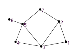
Figure 2:

As particular cases of above theorem we derive the following results in which the expression (31) is simplified.

Corollary 10.

Let $\Gamma=(V,E)$ be a simple and connected graph of order $n$ and size $m$. Let $P_{k}$ be the $k$-alternating polynomial associated to the mesh of the degree-adjacency eigenvalues of $\Gamma$. Then,

$$P_{k}(1)>\frac{2m}{\beta}-1\Rightarrow D^{(\beta,\beta)}(\Gamma)\leq k.$$ (37)

The standard diameter is bounded by

$$P_{k}(1)>\frac{2m}{\delta}-1\Rightarrow D(\Gamma)\leq k.$$ (38)

If $\Gamma$ is regular, the standard diameter is bounded by

$$P_{k}(1)>n-1\Rightarrow D(\Gamma)\leq k.$$ (39)

As we can see in next section, the bound (37) becomes an important tool in the study of the conditional Wiener index. Moreover, the bound (39) is an analogous result to the previous one given by Fiol, Garriga and Yebra in [6] by using the standard adjacency matrix. The reader is referred to [13] for a more general study on the conditional diameter.

6 Conditional Wiener index

The Wiener index $W(\Gamma)$ of a graph $\Gamma$ with vertex set $\{v_{1},v_{2},...,v_{n}\}$ defined as the sum of distances between all pairs of vertices of $\Gamma$,

$$W(\Gamma):=\frac{1}{2}\sum_{i=1,j=1}^{n}\partial(v_{i},v_{j}),$$

is the first mathematical invariant reflecting the topological structure of a molecular graph.

This topological index has been extensively studied, for instance, a comprehensive survey on the direct calculation, applications and the relation of the Wiener index of trees with other parameters of graphs can be found in [5]. Moreover, a list of 120 references of the main works on the Wiener index of graphs can be found in the referred survey.

Alternatively, the Wiener index can be defined as

$$W(\Gamma)=\frac{1}{2}\sum_{v\in V(\Gamma)}S(v),$$

where $S(v)$ denotes the distance of the vertex $v$:

$$S(v):=\sum_{u\in V(\Gamma)}\partial(u,v).$$

We define the conditional Wiener index

$$W_{\wp}(\Gamma):=\frac{1}{2}\sum_{v\in\wp}S_{\wp}(v),$$

where $\wp$ is a property and $v\in\wp$ means that the vertex $v$ satisfies the property $\wp$, and

$$S_{\wp}(v):=\sum_{u\in\wp}\partial(u,v)$$

is the conditional distance of $v$. In particular, if $\wp$ requires that $\delta(v)\geq\beta$, the conditional Wiener index will be denoted by $W_{\beta}(\Gamma)$, moreover, the conditional distance of $v$ will be denoted by $S_{\beta}(v)$. Clearly, if $\beta$ is the minimum degree of $\Gamma$, then $W_{\beta}(\Gamma)$ and the standard Wiener index coincides.

Lemma 11.

The conditional Wiener index of a graph $\Gamma$, $W_{\beta}(\Gamma)$, satisfies

$$W_{\beta}(\Gamma)=\frac{1}{2}\sum_{\delta(v)\geq\beta}\sum_{k=0}^{D^{(\beta,\beta)}(\Gamma)-1}{\bf e}_{k}^{\beta}(v)$$

Proof.

For each vertex $v\in V(\Gamma)$ of degree $\delta(v)>\beta$ we have

$$S_{\beta}(v)=\sum_{k=1}^{D^{(\beta,\beta)}(\Gamma)}k({\bf e}^{\beta}_{k-1}(v)-{\bf e}^{\beta}_{k}(v)).$$

Moreover, by a simple calculation we have

$$S_{\beta}(v)=\sum_{k=0}^{D^{(\beta,\beta)}(\Gamma)-1}{\bf e}^{\beta}_{k}(v).$$ (40)

Hence, by (40) we obtain the result. ∎

Therefore, it follows from Lemma 11 that bounds on ${\bf e}^{\beta}_{k}$ lead to bounds on the conditional Wiener index $W_{\beta}$.

Theorem 12.

Let $\Gamma=(V,E)$ be a simple and connected graph of size $m$. Let $P_{k}$ be the $k$-alternating polynomial associated to the mesh of the degree-adjacency eigenvalues of $\Gamma$ and let $x=\left|\{v\in V(\Gamma):\quad\delta(v)\geq\beta\}\right|$. If $P_{k}(1)>\frac{2m}{\beta}-1$, then

$$W_{\beta}(\Gamma)\leq\frac{x}{2}\displaystyle\sum_{l=0}^{k-1}\left\lfloor\frac{2m(2m-\beta)}{\beta\left(\beta P_{l}^{2}(1)+2m-\beta\right)}\right\rfloor.$$

Proof.

By Lemma 11 and Theorem 7 we have

$$W_{\beta}(\Gamma)\leq\frac{x}{2}\displaystyle\sum_{k=0}^{D^{(\beta,\beta)(\Gamma)-1}}\left\lfloor\frac{2m(2m-\beta)}{\beta\left(\beta P_{k}^{2}(1)+2m-\beta\right)}\right\rfloor.$$ (41)

Therefore, by (37) we conclude the proof. ∎

An analogous upper bound on the standard Wiener index is obtained by replacing, in above theorem, $\beta$ by $\delta$, and $x$ by $n$. Moreover, in the case of regular graphs, the above theorem becomes the following result.

Corollary 13.

Let $\Gamma$ be a simple and connected $\delta$-regular graph of order $n$. Let $P_{k}$ be the $k$-alternating polynomial associated to the mesh of the degree-adjacency eigenvalues of $\Gamma$. If $P_{k}(1)>n-1$, then

$$W(\Gamma)\leq\frac{n}{2}\displaystyle\sum_{l=0}^{k-1}\left\lfloor\frac{n(n-1)}{P_{l}^{2}(1)+n-1}\right\rfloor.$$

The reader is referred to [15] for a more general study on the Wiener index of hypergraphs.

References

• [1] N. Biggs, Algebraic graph theory, Cambridge University Press, 1993.
• [2] B. Bollobás and P. Erdös, Graphs of extremal weights, Ars Combinatoria 50 (1998), 225-233.
• [3] D. M. Cvetković, M. Doob and H. Sachs, Spectra of graphs, Academic Press Inc., New York, 1979.
• [4] K. C. Das and I. Gutman, Some properties of the second Zagreb index, MATCH Commun. Math. Comput. Chem. 52 (2004), 103-112.
• [5] A. A. Dobrynin, R. Entringer and I. Gutman, Wiener Index of Trees: Theory and Applications, Acta Applicandae Mathematicae 66 (2001), 211-249.
• [6] M.A. Fiol, E. Garriga and J.L.A. Yebra, On a class of polynomials and its relation with the spectra and diameters of graphs, J. Combin. Theory Ser. B 67 (1996), 48-61.
• [7] M.A. Fiol and E. Garriga, From local adjacency polynomials to locally pseudo-distance-regular-graphs. J. Combin. Theory Ser. B. 71 (1997), 162-183.
• [8] C. Godsil and G. Royle, Algebraic graph theory, Springer-Verlang New York, Inc. 2001.
• [9] I. Gutman and M. Lepović, Choosing the exponent in the definition of the connectivity, J. Serb. Chem. Soc. 66 (2001), 605-611.
• [10] M. Randić, On the characterization of molecular branching. J. Amer. Chem. Soc. 97 (1975), 6609-6615.
• [11] J. A. Rodríguez and J.L.A. Yebra, Laplacian eigenvalues and the excess of a graph Ars Combinatoria. 64 (2002), 249-258.
• [12] J. A. Rodríguez and J. L. A. Yebra, Cotas espectrales del exceso y la excentricidad de un conjunto de vértices de un grafo. EAMA-97 (1997), 383-390.
• [13] J. A. Rodríguez, The $(\alpha,\beta,s,t)$-diameter of graphs: A particular case of conditional diameter. Discrete Applied Mathematics 154 (14) (2006) 2024–2031.
• [14] J. A. Rodríguez, A spectral approach to the Randić index. Linear Algebra and its Applications 400 (2005) 339–344.
• [15] J. A. Rodríguez, On the Wiener index and the eccentric distance sum of hypergraphs, MATCH Commun. Math. Comput. Chem. 54 (1) (2005) 209–220.