Observational constraints to a phenomenological $f\left(R,\nabla R\right)$-model

Abstract

This paper analyses the cosmological consequences of a modified theory of gravity whose action integral is built from a linear combination of the Ricci scalar $R$ and a quadratic term in the covariant derivative of $R$. The resulting Friedmann equations are of the fifth-order in the Hubble function. These equations are solved numerically for a flat space section geometry and pressureless matter. The cosmological parameters of the higher-order model are fit using SN Ia data and X-ray gas mass fraction in galaxy clusters. The best-fit present-day $t_{0}$ values for the deceleration parameter, jerk and snap are given. The coupling constant $\beta$ of the model is not univocally determined by the data fit, but partially constrained by it. Density parameter $\Omega_{m0}$ is also determined and shows weak correlation with the other parameters. The model allows for two possible future scenarios: there may be either a premature Big Rip or a Rebouncing event depending on the set of values in the space of parameters. The analysis towards the past performed with the best-fit parameters shows that the model is not able to accommodate a matter-dominated stage required to the formation of structure.

¹Instituto de Ciência e Tecnologia, Universidade Federal de Alfenas.
Rod. José Aurélio Vilela (BR 267), Km 533, n^∘11999, CEP 37701-970, Poços de Caldas, MG, Brazil.
²Instituto de Física Teórica, Universidade Estadual Paulista.
Rua Bento Teobaldo Ferraz 271 Bloco II, P.O. Box 70532-2, CEP 01156-970, São Paulo, SP, Brazil.
³Escola de Ciência e Tecnologia, Universidade Federal do Rio Grande do Norte.
Campus Universitário, s/n - Lagoa Nova, CEP 59078-970, Natal, RN, Brazil.
⁴Inst. de Fomento e Coordenação Industrial, Departamento de Ciência e Tecnologia Aeroespacial.
Praça Mal. Eduardo Gomes 50, CEP 12228-901, São José dos Campos, SP, Brazil.
⁵ Instituto Tecnológico de Aeronaútica, Departamento de Ciência e Tecnologia Aeroespacial.
Praça Mal. Eduardo Gomes 50, CEP 12228-900, São José dos Campos, SP, Brazil.

Keywords: Gauge theory, Cosmic acceleration, Higher order gravity, Cosmology.
PACS:98.80.-k, 11.15.-q.

1 Introduction

The cosmological constant is the simplest solution to the problem of the present-day acceleration of the universe. It is consistent with all the available observational tests, from the constraints imposed by CMB maps [1, 2] to BAO picks [3, 4] to SN Ia constraints [5, 6, 7, 8, 9] and the estimates of fraction of baryons in galaxy clusters through X-ray detection [10, 11]. Nevertheless, there is an uncomfortable feeling from the fact that $\Lambda$ is not satisfactory explained as a vacuum state of some field theory: the energy scale observed for $\Lambda$ and predicted by quantum field theory badly disagree [12]. This is one of the reasons why alternative explanations for the present-day cosmic acceleration have been put out since 1998, when it was first detected [13, 14].

These proposals can be classified into two broad categories, each one related to a modification of a different side of the Einstein field equations of General Relativity [15].

The modified matter approach introduces a negative pressure (that counteracts gravity) through the energy momentum tensor $T_{\mu\nu}$ on the right-hand side of Einstein equations. Three types of models constitute this approach, namely quintessence models [16, 17, 18, 19, 20], k-essence solutions [21, 22] and perfect fluid models (such as the Chaplygin gas [23, 24]). The quintessence and k-essence models are based on scalar fields whose potential (in the former case) or the kinetic energy (in the later one) drive the accelerated expansion. The perfect fluid models use exotic equations of state (for the pressure as a function of the energy density) to generate negative pressure. The weakness of k-essence and quintessence proposals lies in the fact that they require a scalar field to be dominant today, when the energy scale is low. This requirement demands the mass of such a field $\phi$ to be extremely small. One would then expect long range interaction of this field with ordinary matter, which is highly constrained by local gravity experiments. The difficulty with the perfect fluid models is the lack of an interpretation to the exotic equations of state based on ordinary physics.

The second approach, called modified gravity, affects the left hand side of Einstein equations [25, 26]. The subtypes of models in this category include braneworld scenarios [27, 28], scalar-tensor theories [29, 30], non-riemannian geometries [31, 32, 33], $f\left(R\right)$ gravity [34, 35, 36, 37, 38, 39] and $f\left(T\right)$ theories [40, 41, 42]. In the braneworld models there exists an additional dimension through which the gravitational interaction occurs and by which the possibility of a cosmic acceleration is accommodated. Scalar-tensor theories couple the scalar curvature $R$ with a scalar field $\phi$ in the action $S$, allowing enough degrees of freedom for an accelerated solution. Non-riemannian geometries are another alternative way to explore the geometrization of the gravitational interaction, but allowing new degrees of freedom describing different geometric structures than curvature. The $f\left(R\right)$ gravity corresponds to models resulting from non-linear Lagrangian densities dependent on $R$; $f\left(T\right)$ theories build their cosmological models on manifolds whose connection is equipped with torsion instead of curvature.

All these mechanisms of generating the present-day cosmic dynamics are generally called dark energy models.

Our aim with the present paper is to contribute with the study of dark energy in the branch of modified gravity. We explore the cosmological consequences of a particular model in the context of the $f\left(R,\nabla R\right)$ gravity testing the model against some of the observational data available. $f\left(R,\nabla R\right)$ gravity is a theory based on an action integral whose kernel is a function of the Ricci scalar $R$ and terms involving derivatives of $R$. Ref. [43] is perhaps an early example of what we call $f\left(R,\nabla R\right)$ gravity. A more recent example is the (non-local) higher derivative cosmology presented in Refs. [44, 45, 46]. These works intend to eliminate the Big Bang singularity through a bounce produced by a theory based on an action containing the regular Einstein-Hilbert term plus a String-spired term. This last ingredient contains an infinite number of derivatives of $R$, a requirement needed to keep this modified gravity theory ghost-free. References [47, 48] are $f\left(R,\nabla R\right)$-gravity prototypes concerned not with the past-incomplete inflationary space-time but with the cosmological constant problem. In this regard, they try to address a similar issue that interests us in the present work: the cosmological acceleration nowadays.

Few years ago, we proposed a gauge theory based on the second order derivative of the gauge potential $A$ following Utiyama’s procedure [49]. This led to a second field strength $G=\partial F+fAF$ (depending on the field strength $F$) and allowed us to obtain massive gauge fields among other applications, such as the study of gauge invariance of the theory under $U(1)$ and $SU(N)$ groups when $\mathcal{L}=\mathcal{L}\left(A,\partial A,\partial^{2}A\right)$. In a subsequent work, gravity was interpreted as a second order gauge theory under the Lorentz group, and all possible Lagrangians with linear and quadratic combinations of $F$ and $G$ – or the Riemann tensor, its derivatives and their possible contractions, from the geometrical point of view – were built and classified within that context [50]. In a third paper we selected one of those quadratic Lagrangians for investigating the cosmological consequences of a theory that takes into account $R$- and $\left(\nabla R\right)^{2}$-terms [51]. That Lagrangian appears in the action $S$ bellow – Eq. (1) – and can be understood as a particular example of an $f\left(R,\nabla R\right)$ gravity:

$$S=\int d^{4}x\sqrt{-g}\left(\frac{R}{2\chi}+\frac{\beta}{8\chi}\nabla_{\mu}R\nabla^{\mu}R-\mathcal{L}_{M}\right)~{},$$ (1)

where $\chi=8\pi G$ (once we take $c=1$), $\beta$ is the coupling constant, $\nabla_{\mu}$ is the covariant derivative, and $\mathcal{L}_{M}$ is the Lagrangian of the matter fields. As usual, $g=\det\left(g_{\mu\nu}\right)$.

An important feature of $S$ is the presence of ghosts (see [46] and references therein). However, here this is not a serious issue because (1) should be considered as an effective action of a fundamental theory of gravity, this last one a ghost-free theory. There are some consistent proposals of extended theories of gravity in the literature. A good example is the String-inspired non-local higher derivative gravitation model presented in Ref. [45]. The ghost-free action of that model is:

$$S=\int d^{4}x\sqrt{-g}\left(\frac{M_{P}^{2}}{2}R+\frac{1}{2}R\mathcal{F}\left(\square/M_{\ast}^{2}\right)R\right)$$ (2)

where $M_{P}$ is the Planck mass ($M_{P}=1/\left(8\pi G\right)$, $G$ is the gravitational constant), $M_{\ast}$ is the mass scale where the higher-derivative terms become important and

$$\mathcal{F}\left(\square/M_{\ast}^{2}\right)={\textstyle\sum\limits_{n=1}^{\infty}}f_{n}\square^{n}~{}.$$ (3)

In this context, our higher-order model must be treated as a low energy limiting case of (2) where the only relevant contribution of Eq. (3) for the present-day universe is the first term of the series, i.e. $f_{1}\gg f_{n}$, $\forall n\geqslant 2$. In this approximation, Eq. (2) is equivalent to the action integral (1) of our $f\left(R,\nabla R\right)$-cosmology up to a surface term. The equivalence of both models leads to a relation between the coupling constant $\beta$ and the parameter $f_{1}$ $\sim$ $M_{\ast}^{-2}$, namely

$$f_{1}=\frac{\beta}{32\pi G}~{}.$$ (4)

Taking the variation of (1) with respect to the metric tensor $g_{\mu\nu}$ (cf. the metric formalism) gives the field equations

$$R_{\mu\nu}-\frac{1}{2}g_{\mu\nu}R+\beta H_{\mu\nu}=\chi T_{\mu\nu}~{},$$ (5)

with

$$H_{\mu\nu} =\nabla_{\mu}\nabla_{\nu}\left[\square R\right]+\frac{1}{2}\nabla_{\mu}R\nabla_{\nu}R$$

$$-R_{\mu\nu}\square R-g_{\mu\nu}\square\left[\square R\right]-\frac{1}{4}g_{\mu\nu}\nabla_{\rho}R\nabla^{\rho}R~{},$$ (6)

where $\square=\nabla_{\mu}\nabla^{\mu}$ and $R_{\mu\nu}$ is the Ricci tensor.

A four dimensional spacetime with homogeneous and isotropic space section is described by the Friedmann-Lemaître-Robertson-Walker (FLRW) line element

$$ds^{2}=c^{2}dt^{2}-a^{2}\left(t\right)\left[\frac{dr^{2}}{1-\kappa r^{2}}+r^{2}\left(d\theta^{2}+\sin^{2}\theta d\phi^{2}\right)\right]~{},$$ (7)

where the curvature parameter $\kappa$ assumes the values $+1,0,-1$ and $a\left(t\right)$ is the scale parameter. Substituting the metric tensor from Eq.(7) along with the energy-momentum tensor of a perfect fluid in co-moving coordinates,

$$T_{\mu\nu}=\left(\rho+P\right)\delta_{\mu}^{\;0}\delta_{\nu}^{\;0}-Pg_{\mu\nu}$$ (8)

($\rho$ is the density and $P$ is the pressure of the components fulling the universe), into the gravity field equations Eq.(5) leads to the two higher order Friedmann equations:

$$H^{2}+\frac{\beta}{3}F_{1}=\frac{8\pi G}{3}\rho~{};$$ (9)

$$3H^{2}+2\dot{H}+\beta F_{2}=-8\pi GP~{},$$ (10)

where

$$F_{1} =18HH^{\left(4\right)}+108H^{2}\dddot{H}-18\dot{H}\dddot{H}+9\ddot{H}^{2}+90H^{3}\ddot{H}$$

$$+216H\dot{H}\ddot{H}-72\dot{H}^{3}+288\left(H\dot{H}\right)^{2}-216H^{4}\dot{H}$$ (11)

$$F_{2} =6H^{(5)}+54HH^{(4)}+138H^{2}\dddot{H}+126\dot{H}\dddot{H}$$

$$+81\ddot{H}^{2}+18H^{3}\ddot{H}+498H\dot{H}\ddot{H}+120\dot{H}^{3}-216H^{4}\dot{H}$$ (12)

which are written in terms of the Hubble function $H=H(t)$,

$$H\equiv\frac{\dot{a}}{a}~{},$$ (13)

and where we have set $\kappa=0$ as is largely favored by the observational data. The dot (such as in $\dot{a}$) means derivative with respect to the cosmic time $t$ and for any arbitrary function of time $f=f(t)$,

$$f^{\left(n\right)}\equiv\frac{d^{n}f}{dt^{n}}~{},$$

i.e., $H^{\left(5\right)}$ is the fifth-order derivative of the Hubble function with respect to the cosmic time.

Eqs. (9) and (10) reduce to the usual Friedmann equations if $\beta\rightarrow 0$. From this system of modified Friedmann equations one can obtain the equation expressing the covariant conservation of the energy momentum tensor, $\nabla_{\nu}T^{\mu\nu}=0$, which reads

$$\dot{\rho}+3H\left(\rho+P\right)=0~{}.$$ (14)

In Ref.[51], we considered simultaneously the set formed by Eq. (14) and a combination of Eqs.(9) and (10), namely

$$\dot{H}+\frac{\beta}{2}\left(F_{2}-F_{1}\right)=-4\pi G\left(\rho+P\right)~{}.$$ (15)

The system of Eqs.(14)-(15) was solved perturbatively with respect to the coupling constant $\beta$ for pressureless matter. Using the observational data available, we have determined the free parameters of our modified theory of gravity and the scale parameter as a function of the time. The plot of $a=a\left(t\right)$ indicates that the decelerated regime peculiar to the universe dominated by matter evolves naturally to an accelerated scenario at recent times.

This makes it promising to perform a more careful analyzes of our $f\left(R,\nabla R\right)$ model making a complete maximum likelihood fit to all parameters.

In this paper we will solve the system of Eqs.(14)-(9) exactly, without using any approximation technique. Section 2 presents the script to obtain the complete solution to the higher order cosmological equations. Another improvement we shall do in the present work (when comparing with Ref.[51]) is to use the observational data available to fully test our model. As far as we know, this is the first time this is done for a higher derivative theory of gravity. In Section 3 we construct the likelihood function to be maximized in the process of fitting the model parameters using data from SN Ia observations [8] and from the measurements of the mass fraction of gas in clusters of galaxies [11]. The results of this fit are given in Section 4, where we show the present-day numerical values for the deceleration parameter $q_{0}=q\left(t_{0}\right)$ [52],

$$q=-\frac{\ddot{a}}{aH^{2}}$$ (16)

the jerk function $j_{0}=j\left(t_{0}\right)$,

$$j=\frac{\dddot{a}}{aH^{3}}~{},$$ (17)

and also of the snap $s_{0}=s\left(t_{0}\right)$,

$$s=\frac{a^{\left(4\right)}}{aH^{4}}~{}.$$ (18)

These last two functions are given in terms of higher-order time derivatives of the scale factor and it is only natural that they show up here. In Section 4.2 we perform an investigation of the dynamical evolution of the model, comparing its behaviour towards the past with the standard solutions for single component universes. Moreover, we show that our $f\left(R,\nabla R\right)$-model accommodates a future Big Rip or a Rebouncing scenario depending on the values of the coupling constant $\beta$. The Rebouncing event is the point where the universe attains its maximum size of expansion and from which it begins to shrink. Our final comments about the features of our model and its validity are given in Section 5.

2 Higher order cosmological model

The solution of our higher-order model shall be obtained from the integration of the pair of Eqs.(9) and (14). The definitions

$$B\equiv H_{0}^{4}\beta~{},$$ (19)

and

$$\Omega_{m}\left(t\right)\equiv\frac{\chi\rho}{3H_{0}^{2}}=\frac{\rho}{\rho_{c}}~{},$$ (20)

enables us to express Eq. (9) as

$$\frac{H^{2}}{H_{0}^{2}}+\frac{B}{3H_{0}^{6}}F_{1}=\Omega_{m}\left(t\right)$$ (21)

and the conservation of energy-momentum Eq.(14) as

$$\dot{\Omega}_{m}+3H\Omega_{m}=0~{},$$ (22)

which is readly integrated:

$$\Omega_{m}=\Omega_{m0}\left(\frac{a_{0}}{a}\right)^{3}~{}.$$ (23)

It is standard to take $a_{0}=1$. Moreover, substituting the solution (23) into Eq. (21), leads to a fifth-order differential equation in $a$:

$$\frac{1}{H_{0}^{2}}\dot{a}^{2}a^{4}+\frac{B}{H_{0}^{6}}\mathcal{F}_{1}=\Omega_{m0}a^{3}$$ (24)

with

$$\mathcal{F}_{1} =6a^{\left(5\right)}\dot{a}a^{4}-6a^{\left(4\right)}\ddot{a}a^{4}+12a^{\left(4\right)}\dot{a}^{2}a^{3}$$

$$+3~{}\dddot{a}^{2}a^{4}+18\dddot{a}\ddot{a}\dot{a}a^{3}-78\dddot{a}\dot{a}^{3}a^{2}$$

$$-6\ddot{a}^{3}a^{3}-39\ddot{a}^{2}\dot{a}^{2}a^{2}+78\ddot{a}\dot{a}^{4}a-180\dot{a}^{6}$$ (25)

In order to solve Eq. (24), we define the non-dimensional variables

$$\mathcal{H} \equiv\frac{\dot{a}}{H_{0}}=a\frac{H}{H_{0}}~{};$$ (26)

$$Q \equiv\frac{\mathcal{\dot{H}}}{H_{0}}=-a\frac{H^{2}}{H_{0}^{2}}q~{};$$ (27)

$$J \equiv\frac{\dot{Q}}{H_{0}}=a\frac{H^{3}}{H_{0}^{3}}j~{};$$ (28)

$$S \equiv\frac{\dot{J}}{H_{0}}=a\frac{H^{4}}{H_{0}^{4}}s~{},$$ (29)

which are related to the Hubble function, deceleration parameter, jerk and snap. In fact, when these variables are calculated at the present time, $t=t_{0}$, they give precisely the well known cosmological parameters: $\mathcal{H}\left(t_{0}\right)=\mathcal{H}_{0}=a_{0}=1$, $Q_{0}=-q_{0}$, $J_{0}=j_{0}$ and $S_{0}=s_{0}$. In the set of variables (26)-(29), one variable is essentially the derivative of the previous one, therefore they can be used to turn the fifth-order differential equation Eq.(24) into five first order differential equations to be solved simultaneously. Following the Method of Characteristics, we choose the scale factor $a$ as the independent variable of the model (instead of the cosmic time $t$), obtaining the system

$$\left\{\begin{array}[c]{l}\frac{d\mathcal{H}}{dz}=-\frac{1}{\left(1+z\right)^{2}}\frac{Q}{\mathcal{H}}\\ \frac{dQ}{dz}=-\frac{1}{\left(1+z\right)^{2}}\frac{J}{\mathcal{H}}\\ \frac{dJ}{dz}=-\frac{1}{\left(1+z\right)^{2}}\frac{S}{\mathcal{H}}\\ \frac{dS}{dz}=\frac{-1}{\left(1+z\right)^{2}}F_{3}\left(z;\mathcal{H},Q,J,S\right)\end{array}\right.~{},$$ (30)

with

$$F_{3}\left(z;\mathcal{H},Q,J,S\right) =-2S\left(1+z\right)+\frac{SQ}{\mathcal{H}^{2}}$$

$$-\frac{1}{2}\left(\frac{J}{\mathcal{H}}\right)^{2}-3\frac{JQ\left(1+z\right)}{\mathcal{H}}+13J\mathcal{H}\left(1+z\right)^{2}$$

$$+\frac{Q^{3}\left(1+z\right)}{\mathcal{H}^{2}}+\frac{13}{2}Q^{2}\left(1+z\right)^{2}-13Q\mathcal{H}^{2}\left(1+z\right)^{3}$$

$$+30\mathcal{H}^{4}\left(1+z\right)^{4}+\frac{\Omega_{m0}}{6B}\frac{\left(1+z\right)}{\mathcal{H}^{2}}-\frac{1}{6B}~{},$$ (31)

where we have used the relationship between the redshift and the scale factor,

$$\left(1+z\right)=\frac{1}{a}~{}.$$ (32)

The system of Eq.(30) is solved numerically, which is indeed a far more simpler task than dealing directly with Eq. (24). This leads to a function $\mathcal{H}\left(z\right)$ (essentially equal to $\dot{a}$) for each set $[\mathcal{M}]=\{q_{0},j_{0},s_{0},B,\Omega_{m0}\}$ of cosmological parameters. This function is used to obtain an interpolated function for the luminosity distance $d_{L}=d_{L}\left(z,[\mathcal{M}]\right)$ of our model – defined bellow – which is to be fitted to the data from SN Ia observations and from $f$-gas measurements.

3 Fitting the model to the SN Ia and $f$-gas data

3.1 SN Ia data

In order to relate the proposed model to the observational data, one has to build the luminosity distance $d_{L}$ [15],

$$d_{L}=\left(1+z\right){\displaystyle\int\limits_{0}^{z}}\frac{d\bar{z}}{H\left(\bar{z}\right)}=\frac{\left(1+z\right)}{H_{0}}{\displaystyle\int\limits_{0}^{z}}\frac{d\bar{z}}{\left(1+\bar{z}\right)~{}\mathcal{H}\left(\bar{z}\right)}~{}.$$ (33)

Our task is to solve the system Eq.(30) for obtaining $\mathcal{H}$, then to integrate numerically the non-dimensional luminosity distance,

$$d_{h}\left(z;[\mathcal{M}]\right)=\frac{H_{0}}{c}d_{L}\left(z;[\mathcal{M}]\right)~{},\;\;\;\;\;\;\left(c=1\right)$$ (34)

for each set of cosmological parameters $[\mathcal{M}]=\{q_{0},j_{0},s_{0},B,\Omega_{m0}\}$.

Function $d_{h}$ appears in the definition of the distance modulus,

$$\mu_{r}=5\log_{10}d_{h}+5\log_{10}\left(\frac{c}{H_{0}d_{0}}\right)~{},$$ (35)

where $d_{0}$ is the reference distance of $10$ pc. Observational data give $\mu_{r}$ of the supernovae and their corresponding redshift $z$.

According to the likelihood method the probability distribution of the data

$$\mathcal{L}_{SNIa}\left(\left[\mathcal{M}\right]|\left\{z_{i},\mu_{r_{i}}\right\}\right)=N_{SNIa}e^{-\frac{\chi_{SNIa}^{2}\left(\mathcal{[M]}\right)}{2}}$$ (36)

($N_{SNIa}$ is a normalization constant) is the one that minimizes

$$\chi_{SNIa}^{2}\left([\mathcal{M}]\right)={\displaystyle\sum\limits_{i}}\frac{\left(\mu_{r_{i}}-5\log d_{h}\left(z_{i},[\mathcal{M}]\right)-5\log_{10}\left(\frac{c}{H_{0}d_{0}}\right)\right)^{2}}{\sigma_{\mu_{i}}^{2}+\sigma_{ext}^{2}}~{},$$ (37)

where $\sigma_{\mu_{i}}$ is the uncertainty related to the distance modulus $\mu_{r_{i}}$ of the $i$-th supernova. The data set used in our calculations is composed with the 557 supernovae of the Union 2 compilation [8]. Uncertainty $\sigma_{ext}$ is given by

$$\sigma_{ext}^{2}=\sigma_{\mu_{v}}^{2}+\sigma_{lens}^{2}~{},$$ (38)

i.e., it is the combination of the error $\sigma_{v}$ in the magnitude due to host galaxy peculiar velocities (of order of $300\operatorname{km}\operatorname{s}^{-1}$),

$$\sigma_{\mu_{v}}=\frac{2.172}{z}\frac{\sigma_{v}}{c}\text{\ \ \ with\ \ \ }\sigma_{v}=300\operatorname{km}\operatorname{s}^{-1}~{},$$ (39)

and the uncertainty from gravitational lensing

$$\sigma_{lens}=0.093z$$ (40)

which is progressively important at increasing SN redshifts. Further detail can be found in Refs. [53, 54], for example.

3.2 Galaxy cluster X-ray data

Measurements of the fraction of the mass of gas in galaxy clusters in the X-ray band of the spectrum constrain efficiently the ratio $\frac{\Omega_{b0}}{\Omega_{m0}}$ and exhibit a lower dependence on the values of other cosmological parameters [10, 11]. According to Ref.[11], the mass fraction of gas $f_{gas}$ relates to $\frac{\Omega_{b0}}{\Omega_{m0}}$ as

$$f_{gas}^{\Lambda CDM}\left(z\right)=\frac{KA\gamma b\left(z\right)}{1+s\left(z\right)}\left(\frac{\Omega_{b0}}{\Omega_{m0}}\right)\left[\frac{d_{A}^{\Lambda CDM}\left(z\right)}{d_{A}\left(z\right)}\right]^{1,5}~{},$$ (41)

where $d_{A}$ is the angular distance for $\kappa=0$,

$$d_{A}\left(z\right)=\frac{d_{L}\left(z\right)}{\left(1+z\right)^{2}}=\frac{1}{\left(1+z\right)}\frac{1}{H_{0}}{\displaystyle\int\limits_{0}^{z}}\frac{d\bar{z}}{\left(1+\bar{z}\right)\mathcal{H}\left(\bar{z};[\mathcal{M}]\right)}~{}.$$ (42)

The term $d_{A}^{\Lambda CDM}\left(z\right)$ is the angular distance for the standard $\Lambda$CDM model, for which $\Omega_{m0}=0.3$, $\Omega_{\Lambda}=0.7$ and $H_{0}^{70}=70\operatorname{km}\operatorname{s}^{-1}$Mpc^-1, i.e.

$$d_{A}^{\Lambda CDM}\left(z\right)=\frac{1}{\left(1+z\right)}\frac{1}{H_{0}}{\displaystyle\int\limits_{0}^{z}}\frac{d\bar{z}}{\left[\Omega_{m0}\left(1+\bar{z}\right)^{3}+\Omega_{\Lambda}\right]^{1/2}}.$$ (43)

The other factors in Eq. (41) are defined bellow:

• $K$ is a constant due to the calibration of the instruments observing in X-ray. Following Ref. [11], we take $K=1.0\pm 0.1$.

• Constant $A$ measures the angular correction on the path of an light ray propagating in the cluster due to the difference between $\Lambda$CDM model and the model that we want to fit to the data. Ref. [11] argues that for relatively low red-shifts (as those involved here) this factor can be neglected, i.e. taken as $A=1$.

• $\gamma$ accounts for the influence of the non-thermal pressure within the clusters. According to Ref.[11], one may set $1.0<\gamma<1.1$. Our choice is $\gamma=1.050\pm 0.029$.

• $b\left(z\right)$ is the bias factor related to the thermodynamical history of the inter-cluster gas. Once again due to arguments given in Ref.[11], this factor can be modeled as $b\left(z\right)=b_{0}\left(1+\alpha_{b}z\right)$ where $b_{0}=0.83\pm 0.04$ and $-0.1<\alpha_{b}<0.1$. We set $\alpha_{b}=0.000\pm 0.058$.

• Parameter $s\left(z\right)=s_{0}\left(1+\alpha_{s}z\right)$ describes the fraction of baryonic mass in the stars. Ref. [11] uses $s_{0}=\left(0.16\pm 0.05\right)h_{70}^{1/2}$ and $-0.2<\alpha_{s}<0.2$. Here

  $$h_{70}=\frac{H_{0}}{H_{0}^{70}\text{ }}~{},$$ (44)

  and we will set $\alpha_{s}=0.000\pm 0.115$. Analogously to Eq.(44), we define

  $$h=\frac{H_{0}}{\left(100\operatorname{km}\operatorname{s}^{-1}Mpc^{-1}\right)}~{},$$ (45)

  that will be required bellow.

• The baryon parameter $\Omega_{b0}$ is set to

  $$\Omega_{b0}h^{2}=0.0214\pm 0.002$$ (46)

  following the constraints imposed by the primordial nucleosynthesis on the ratio $D/H$ [55].

The uncertainties in the set of parameters $\{b_{0},s_{0},K,\Omega_{b0}h^{2},\alpha_{s},\alpha_{b},\gamma\}$ are propagated to build the uncertainty of $f_{gas}^{\Lambda CDM}$. It is worth mentioning that the quantities $\left\{b_{0},s_{0},K,\Omega_{b0}h^{2}\right\}$ have Gaussian uncertainties. On the other hand, the parameters $\left\{\alpha_{s},\alpha_{b},\gamma\right\}$ present a rectangular distribution, e.g. $\gamma$ has equal probability of assuming values in the interval $\left[1.0,1.1\right]$. The uncertainty of the parameters obeying the rectangular distribution is estimated as the half of their variation interval divided by $\sqrt{3}$. Maybe it is useful to remark that in the case of $s_{0}$, we adopted $h_{70}^{1/2}\simeq 1$. Moreover, $\frac{h^{2}}{h_{70}^{2}}=\left(\frac{0.7}{1}\right)^{2}\cong 0.49$.

Ref. [11] provides data for the fraction of gas $f_{gas}$ and its uncertainty $\sigma_{f}$ of 42 galaxy clusters with redshift $z$. These data can be used to determine the free parameter of our model by minimizing

$$\chi_{gas}^{2}\left([\mathcal{M}]\right)={\displaystyle\sum\limits_{i}}\frac{\left(f_{gas}^{i}-f_{gas}^{\Lambda CDM}\left(z,[\mathcal{M}]\right)\right)^{2}}{\sigma_{f_{i}}^{2}}$$ (47)

Notice that the dependence of $\chi^{2}$ on the set $\left[\mathcal{M}\right]$ of cosmological parameters occurs through the function $f_{gas}^{\Lambda CDM}$ given by Eq.(41), i.e. ultimately through $d_{A}\left(z,\left[\mathcal{M}\right]\right)$ – Eq. 42.

Function $\chi_{gas}^{2}$ is related to the distribution

$$\mathcal{L}_{gas}\left(\left[\mathcal{M}\right]\right)=N_{gas}e^{-\frac{\chi_{gas}^{2}\left(\mathcal{[M]}\right)}{2}}$$ (48)

which should be maximized.

3.3 Combining SN Ia and $f$-gas data sets

The majority of papers that present cosmological models tested through SN Ia data fit – see e.g. Refs. [20, 53] – perform an analitical marginalization with respect to $H_{0}$. On the other hand, constraint analyses using $f$-gas data adopt a fixed value for $H_{0}$. Our basic reference on $f$-gas treatment, namely Ref.[11], choose $H_{0}=70\operatorname{km}\operatorname{s}^{-1}$Mpc^-1. As we will consider SN Ia and $f$-gas data sets in the same footing, it is convenient to adopt $H_{0}=70\operatorname{km}\operatorname{s}^{-1}$Mpc^-1 as a fixed quantity in our calculations (and not the most up-to-date value of $\left(73.8\pm 2.4\right)\operatorname{km}\operatorname{s}^{-1}$Mpc^-1 found in [56]).

We want to maximize the probability distributions given in Eqs.(36) and (48) simultaneously, which is done by maximixing

$$\mathcal{L}\left(\left[\mathcal{M}\right]\right)=\mathcal{L}_{SNIa}\left(\left[\mathcal{M}\right]\right)\mathcal{L}_{gas}\left(\left[\mathcal{M}\right]\right)~{},$$ (49)

or minimizing

$$\chi^{2}\left([\mathcal{M}]\right)=\chi_{SNIa}^{2}\left([\mathcal{M}]\right)+\chi_{gas}^{2}\left([\mathcal{M}]\right)~{}.$$ (50)

4 Results

4.1 Estimation of the free parameters of the $f\left(R,\nabla R\right)$-model

The parameters to be ajusted are of two types. The kinematic parameters are $\left\{q_{0},j_{0},s_{0}\right\}$; the cosmological parameters are $\left\{\Omega_{m0},B\right\}$. Maximization of the likelihood function $\mathcal{L}\left(\left[\mathcal{M}\right]\right)$ – Eq. (49) – determines all kinematic parameters and one cosmological parameter, namely $\left\{q_{0},j_{0},s_{0},\Omega_{m0}\right\}$. Parameter $B$ is not fixed by statistical treatment of the data, and the reason for that is evident in the plot of Fig. 1.

Figure 1: Sketch of the likelihood function $\mathcal{L}\left(\left[\mathcal{M}\right]\right)$ as a function of the absolute value of the coupling parameter $B$. The other parameters $\left\{q_{0},j_{0},s_{0},\Omega_{m0}\right\}$ were fixed in their best-fit values.

The curve of $\mathcal{L}\left(\left|B\right|\right)$ is not Gaussian but rather shows a flat region at high values of $\left|B\right|$. Indeed, values of $\left|B\right|$ greater than $10^{-3}$ are almost equally probable and more favorable than the $\left|B\right|<10^{-3}$. This shows it is not possible to determine $B$ by maximizing its likelihood function. Instead, we choose four values of $B$ to proceed the analysis leading to the determination of the free parameters of the model. These values are $B=\left(\pm 10^{-3},\pm 10^{-1}\right)$, so that we have two values of $B$ in the beginning of the plateau ($\left|B\right|=10^{-3}$) and two of them far from the beginning of the plateau ($\left|B\right|=10^{-1}$). These choices are only partially arbitrary: we have done preliminary calculations with other values of $\left|B\right|$ ($\left|B\right|=1,10,100$) and the results for the best-fit calculations of $\left\{q_{0},j_{0},s_{0},\Omega_{m0}\right\}$ are almost the same as those obtained by using $\left|B\right|=10^{-1}$.

The standard statistical analysis leads to the best-fit values of the parameters shown in Table 1.

Table 1: Fit results of the parameters of our $f\left(R,\nabla R\right)$-model. The uncertainties represent a 68% confidence level (CL).

$B$	$q_{0}$	$j_{0}$	$s_{0}$	$\Omega_{m0}$
$-10^{-1}$	$-0.51_{-0.14}^{+0.14}$	$0.3_{-2.5}^{+1.7}$	$0.4_{-11.1}^{+9.3}$	$0.301_{-0.010}^{+0.010}$
$-10^{-3}$	$-0.55_{-0.14}^{+0.14}$	$1.4_{-2.2}^{+2.1}$	$18.5_{-11.0}^{+9.8}$	$0.301_{-0.010}^{+0.011}$
$+10^{-3}$	$-0.46_{-0.14}^{+0.14}$	$-1.6_{-2.1}^{+2.1}$	$-19.4_{-10.3}^{+9.7}$	$0.301_{-0.010}^{+0.010}$
$+10^{-1}$	$-0.51_{-0.14}^{+0.14}$	$0.3_{-2.5}^{+1.7}$	$0.4_{-11.0}^{+9.3}$	$0.301_{-0.010}^{+0.010}$

It is clear from Table 1 that our higher order cosmological model presents an acceleration at present time: the deceleration parameter $q_{0}$ is negative for all the values of the coupling constant $B$. This is a robust result indeed once we have got negative values for $q_{0}$ with $99.7\%$ confidence level.

Both SN Ia and $f$-gas data sets give information about astrophysical objects at relatively low redshifts ($z\lesssim 1.4$). That is the reason for the high values of the uncertainties on the parameter $j_{0}$ and $s_{0}$. Positive values of $j_{0}$ mean that the tendency is the increasing of the rate of cosmic acceleration. Because the jerk parameter $j_{0}$ does not exhibit the same sign for all values of $B$, it is not possible to argue in favor of an overall behavior for the cosmic acceleration today. This statement is also applicable to the snap $s_{0}$ obtained with $B=\pm 10^{-1}$. However, the uncertainties in the value of $s_{0}$ for $B=-10^{-3}$ do indicate that it is positive within 68% CL. The negative value of $s_{0}$ for $B=+10^{-3}$ is also guaranteed within the same CL. This difference in the sign of $s_{0}$ for $B=-10^{-3}$ and $B=+10^{-3}$ leads to distinct dynamics for the scale factor towards the future, as we shall discuss in Section 4.2.

The best-fits for $\Omega_{m0}$ are statistically the same for all the chosen values of $B$. This is linked to the fact that the $f$-gas data produce a sharp determination of this parameter. Notice that the value $\Omega_{m0}$ of our model is compatible with that of $\Lambda$CDM model as reported in Ref.[8] within 95% CL. Inspection of Table 1 indicates that the Gaussian-like distributions centered in each parameter of the set $\left\{q_{0},j_{0},s_{0},\Omega_{m0}\right\}$ for $B=-10^{-1}$ overlap the distributions centered in $\left\{q_{0},j_{0},s_{0},\Omega_{m0}\right\}$ for $B=+10^{-1}$; this overlap of distribution curves occurs within 68% CL of each distribution. Moreover, this overlap of distributions is greater than the one observed in the case of the sets $\left\{q_{0},j_{0},s_{0},\Omega_{m0}\right\}$ for $B=-10^{-3}$ and $B=+10^{-3}$, which occurs within 95% CL. Hence, the greater the value of $\left|B\right|$, the greater the overlap of distribution and the less important is our choice of the value of $B$. This emphasizes what was said before about the choice of values for $B$.

The confidence regions (CR) in the $\left(q_{0},j_{0}\right)$ and $\left(q_{0},\Omega_{m0}\right)$ planes for each one of the four values of $B$ are shown in Figs. 2-5.

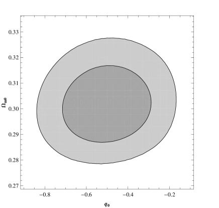
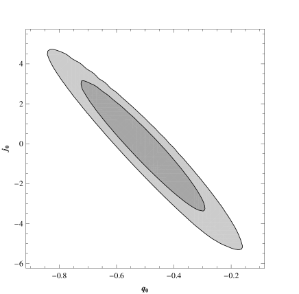
Figure 2: Confidence regions in the $\left(q_{0},\Omega_{m0}\right)$ and $\left(q_{0},j_{0}\right)$ planes for $B=-10^{-1}$ from SN Ia and $f$-gas data sets. The inner contour contains the 68% CR, whilst the outer curves confines the 95% CR.

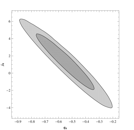
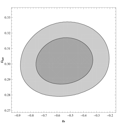
Figure 3: 68% and 95% confidence regions in the $\left(q_{0},j_{0}\right)$ and $\left(q_{0},\Omega_{m0}\right)$ planes for $B=-10^{-3}$.

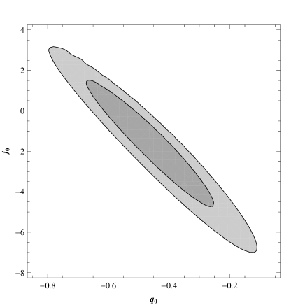
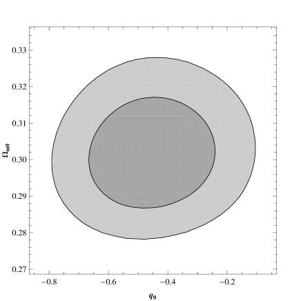
Figure 4: Confidence regions in the plots $\left(q_{0},j_{0}\right)$ and $\left(q_{0},\Omega_{m0}\right)$ planes for the value $B=+10^{-3}$ of the coupling constant.

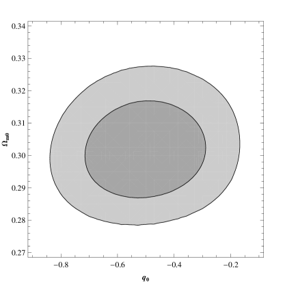
Figure 5: CR in the planes $\left(q_{0},j_{0}\right)$ and $\left(q_{0},\Omega_{m0}\right)$ for $B=+10^{-1}$.

The shape of the confidence regions for $\left(q_{0},j_{0}\right)$ indicates that the deceleration parameter $q_{0}$ and the jerk $j_{0}$ are correlated parameters; this occurs for all the values of $B$. The four plots $\left(q_{0},j_{0}\right)$ point to an accelerated universe at recent times within 95% CL, but the change in the acceleration rate takes positive and negative values with equal probability.

Conversely, the shape of the plots of $\left(q_{0},\Omega_{m0}\right)$ in Figs. 2–5 indicate that $q_{0}$ and $\Omega_{m0}$ are weakly correlated parameters. Notice that the difference between the maximum and the minimum values of $\Omega_{m0}$ in the range of the plots $q_{0}\times\Omega_{m0}$ is only 0.05 with 95% CL: this confirms that the parameter $\Omega_{m0}$ is sharply determined by the best-fit procedure (something that is consistent with the fact that we have employed $f$-gas data to build the likelihood function).

In order to quantify the correlation between the parameters $\left(q_{0},\,j_{0}\right)$ and $\left(q_{0},\,\Omega_{m0}\right)$, the covariances $\sigma_{q_{0}j_{0}}$, $\sigma_{q_{0}\Omega_{m0}}$ and correlation coefficients $r_{q_{0}j_{0}}$, $r_{q_{0}\Omega_{m0}}$ were evaluated according to Ref. [57]. The mean values and their respective standard deviations used to calculate the covariances and correlation coefficients were those given in Table 2. The same table shows the values obtained for the covariances and correlation functions for each value of $B$ taken in this paper.

Table 2: Values of mean and standard deviation of the parameters $\left\{q_{0},j_{0},\Omega_{m0},s_{0}\right\}$ for different values of $B$. The values of $s_{0}$, although irrelevant for the evaluation of the parameters of interest, were included for completeness. The last four columns show the values of covariances $\sigma_{q_{0}j_{0}}$, $\sigma_{q_{0}\Omega_{m0}}$ and correlation coefficients $r_{q_{0}j_{0}}$, $r_{q_{0}\Omega_{m0}}$.

$B$	$q_{0}$	$j_{0}$	$\Omega_{m0}$	$s_{0}$	$\sigma_{q_{0}j_{0}}$	$r_{q_{0}j_{0}}$	$\sigma_{q_{0}\Omega_{m0}}$	$r_{q_{0}\Omega_{m0}}$
$-10^{-1}$	$-0.50\pm 0.14$	$-0.2\pm 2.1$	$0.302\pm 0.010$	$-1.5\pm 9.8$	$-0.269$	$-0.954$	$0.00011$	$0.0817$
$-10^{-3}$	$-0.54\pm 0.14$	$1.2\pm 2.1$	$0.299\pm 0.010$	$17\pm 10$	$-0.267$	$-0.952$	$0.00012$	$0.0812$
$+10^{-3}$	$-0.45\pm 0.14$	$-1.7\pm 2.1$	$0.302\pm 0.010$	$-20.9\pm 9.9$	$-0.272$	$-0.956$	$0.00011$	$0.0753$
$+10^{-1}$	$0.50\pm 0.14$	$-0.2\pm 2.1$	$0.302\pm 0.010$	$-1.5\pm 9.9$	$-0.258$	$-0.954$	$0.00011$	$0.0817$

The values of the correlation coefficient presented in Table 2 confirm what was stated before: The parameters $q_{0}$ and $j_{0}$ are strongly (negatively) correlated while $q_{0}$ and $\Omega_{m0}$ are weakly correlated for all values of B considered here.

Comparison of the results presented in Table 2 and Table 1 shows that there is no statistical difference between considering the mode and a confidence interval of 68% (Table 1) from taking the mean and standard deviation. This emphasizes the quasi-gaussian behaviour of the probability function.

4.2 Behaviour of the $f\left(R,\nabla R\right)$-model with time

We can investigate the evolution of our higher order model in time by plotting the function $\mathcal{H}=\dot{a}/H_{0}$ as a function of $z$. This is done setting the parameters at their best-fit results for each value of $B$.

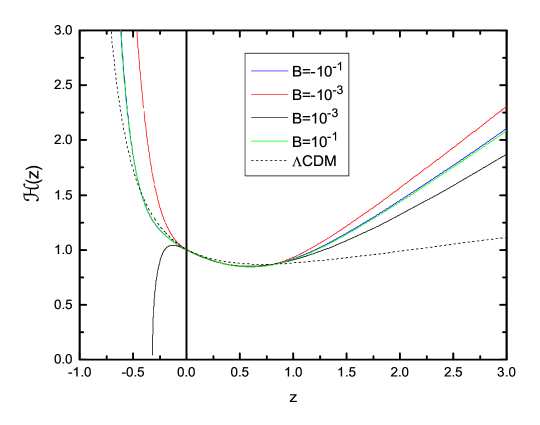
Figure 6: Plot of the function $\mathcal{H}\left(z\right)$ accounting for the best-fit parameters of the higher order model. This is essentially the curve of $\dot{a}$ as a function of $z$ for our model – colored lines – and for the standard $\Lambda$CDM model – dashed line. The notation is: $B=-10^{-1}$ is the blue curve; $B=-10^{-3}$, red line; $B=+10^{-3}$, black curve; and $B=+10^{-1}$, green line.

There is agreement between our model – regardless the value of $B$ – and the standard $\Lambda$CDM model in the region $0\lesssim z\lesssim 1$. In particular, the curves of $\mathcal{H}\left(z\right)$ for $B=-10^{-1}$ and $B=+10^{-1}$ almost coincide: the difference between them is only noticeable at $z\simeq 3$. The transition from a decelerated phase to an accelerated expansion in the higher order model occurs at $z\simeq 0.6$ for all values of $B$.

Towards the future ($t>t_{0}$) the redshift takes negative values, $-1<z<0$. In this region our model present different dynamics depending on the value of the coupling constant. For $B=-10^{-1}$, $B=-10^{-3}$ and $B=+10^{-1}$, there is an onset of an ever growing acceleration eventually leading to a premature Big Rip, respective to the one taking place in the $\Lambda$CDM model. On the other hand, the velocity in the higher order model with $B=+10^{-3}$ – black curve in Fig. 6 – reaches a maximum value at $z\simeq-0.15$, the acceleration then changes the sign, leading to a positive deceleration parameter. This deceleration is sufficiently intense to produce a Rebouncing, where the universe reaches a maximum size and then begins to shrink. This happens at $z\simeq-0.32$.

This difference between Big Rip and Rebouncing scenarios deserves a more careful statistical analysis. We shall consider this in a broader space of parameters, and not using only the best-fit values for the parameters of our model, as we have done so far. A careful analysis shows that the deceleration parameter $q_{0}$ influences weakly on the possible future regimes of our model. The parameters that decisively decide in favor of a Big Rip scenario or a Rebouncing event are the jerk $j_{0}$ and the snap $s_{0}$. Fig. 7 displays the $\left(j_{0},s_{0}\right)$ confidence regions plots for $B=\pm 10^{-1}$.

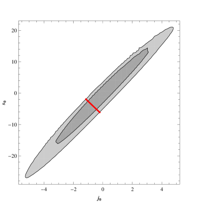
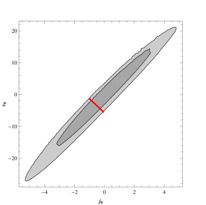
Figure 7: $\left(j_{0},s_{0}\right)$ confidence regions for $B=-10^{-1}$ (left) and $B=+10^{-1}$ (right) with $q_{0}$ and $\Omega_{m0}$ set to their best-fit values.

The straight red lines passing through the confidence regions of the plots Fig. 7 separate the sector of the space of parameters where the Rebouncing occurs (lower part) from that region of values corresponding to a Big Rip (upper part). A numerical analysis shows that 39% of the $\left(j_{0},s_{0}\right)$ confidence region allows for the Rebouncing scenario in the higher order model with $B=-10^{-1}$ and 42% of the confidence region for the model with $B=+10^{-1}$ leads to Rebouncing. A similar analysis shows that the model with $B=-10^{-3}$ produces a premature Big Rip for all the values of the pair $\left(j_{0},s_{0}\right)$ in the 95% confidence region; converselly, the model with $B=+10^{-3}$ engenders Rebouncing within the 95% CR.

At last, it is interesting to explore the features of the model for $z\gtrsim 1$. Extrapolating the results presented in Fig. 6 we verified that our model does not reproduce the decelerated phase typical of a matter dominated Friedmann universe. Besides, for $10\lesssim z\lesssim 1000$ the higher order model exhibits a behaviour compatible with

$$\frac{1}{3}<\omega<\frac{1.25}{3}\;,$$ (51)

where the equation of state is $P=\omega\rho$, i.e. the equation for a perfect fluid in the standard Friedmann cosmology. On the other hand, a linear perturbative analysis shows that the perturbations in gravitation and matter fields do not grow for the equation of state with $\omega$ as given in (51). Therefore, the model proposed here can not describe the structure formation in the early universe.

5 Final Remarks

In this paper we have studied the phenomenological features of a particular modified gravity model built with an action integral dependent on the Ricci scalar $R$ and also on the contraction $\nabla_{\mu}R\nabla^{\mu}R$ of its covariant derivatives. The Friedmann equations resulting from the field equation and the FLRW line element involve sixth-order time-derivatives of the scale factor $a$. We solved those differential equations numerically – but without any approximation – assuming a null cuvature parameter ($\kappa=0$) and pressureless matter. Our higher order model depends on five parameters, namely $\left[\mathcal{M}\right]=\left\{q_{0},j_{0},s_{0},\Omega_{m0};B\right\}$. The present day value of the Hubble constant is taken as given – and not constrained by data fit – the reason for that being consistency with the $f$-gas data analysis. Four of the five parameters $\left[\mathcal{M}\right]$ are determined by the best-fit to the data for the SN Ia $d_{L}\left(z\right)$ and fraction of gas in galaxy clusters $d_{A}\left(z\right)$ available from Refs.[8] and [11], respectively.

The shape of the likelihood function $\mathcal{L}$ in terms of $B$ shows that it is not possible to determine this parameter by maximization. We were forced to select some values of $B$ and proceed to the best-fit of the other parameters in the set $\left[\mathcal{M}\right]$. It was clear that the $\Omega_{m0}$ is statistically independent of the initial conditions, regardless the values of $B$ and the other best-fit parameters. In addition the sign of both $j_{0}$ and $s_{0}$ depend on $B$, so that the behaviour of the model towards the future is not unique.

The confidence regions for the pair of parameters $\left(q_{0},j_{0}\right)$, $\left(q_{0},\Omega_{m0}\right)$ and $\left(j_{0},s_{0}\right)$ were built. They showed that $q_{0}$ and $j_{0}$ are strongly correlated parameters, whereas $q_{0}$ and $\Omega_{m0}$ are weakly correlated quantities. This was confirmed by the results in Table 2. The plot of the confidence region for the pair $\left(j_{0},s_{0}\right)$ is relevant to understand the future evolution of our higher-order model, which can exhibit either a premature Big Rip or a Rebouncing depending on the value of $B$ and on the values of $j_{0}$ and $s_{0}$.

If additional data for high $z$ objects were used, as Gamma Ray Bursts, for instance, they might reduce the uncertainties in our estimations of the jerk and the snap, and help us to decide if the Rebouncing scenario is favored with respect to the Big Rip, or conversely.

A positive feature of the particular $f\left(R,\nabla R\right)$-model presented here is its consistency with the standard $\Lambda$CDM dynamics at recent times. Maybe this is anticipated because the model has a great number of free parameters to be fit to the data. The high number of kinematic parameters (i.e., those involving acceleration and its first and second derivatives) is a consequence of the model being of the fifth-order in derivatives of $H$, a fact that could always make room for agreement with the observations. However, the freedom for bias is not unlimited. Even with all these free parameters there is a constraint to the dynamics of the model towards the past.

Besides this consistency with the standard $\Lambda$CDM dynamics (at recent times) the model does not reproduce a large scale structure formation phase. This shows that just fitting a model to actual data is not enough to falsify or prove the model. General essential characteristic must be present too, as the instabilities allowing the large scale structure formation. Therefore, the extra term presented in the action (1) should be ruled out as viable alternative for dark energy.

Acknowledgements

This paper is dedicated to Prof. Mario Novello on the ocasion of his 70th birthday. RRC thanks FAPEMIG-Brazil (grant CEX–APQ–04440-10) for financial support. CAMM is grateful to FAPEMIG-Brazil for partial support. LGM acknowledges FAPERN-Brazil for financial support.

References

- [1] D. N. Spergel et al., First year Wilkinson Microwave Anisotropy Probe (WMAP) observations: Determination of cosmological parameters, Astrophys. J. Suppl. 148 (2003), 175; E. Komatsu et al., Seven-year Wilkinson Microwave Anisotropy Probe (WMAP) observations: Cosmological interpretation, Astrophys. J. Suppl. 192:18 (2011).
- [2] Planck Collaboration: P. A. R. Ade et al., Planck 2013 results. I. Overview of products and scientific results, arXiv: 1303.5062 (2013); Planck Collaboration: P. A. R. Ade et al., Planck 2013 results. XVI. Cosmological parameters, arXiv: 1303.5076 (2013).
- [3] D. J. Eisenstein et al., Detection of the Barion Acoustic Peak in the large-scale correlation function of SDSS luminous red galaxies, Astrophys. J. 633 (2005), 560; W. J. Percival et al., Baryon Acoustic Oscillations in the Sloan Digital Sky Survey Data Release 7 Galaxy Sample, Mon. Not. Roy. Astron. Soc. 401 (2010), 2148.
- [4] S. Cole et al., The 2dF Galaxy Redshift Survey: Power-spectrum analysis of the final dataset and cosmological implications, Mon. Not. Roy. Astron. Soc. 362 (2005), 505; F. Beutler, The 6dF Galaxy Survey: Baryon Acoustic Oscilations and the local Hubble constant, Mon. Not. Roy. Astron. Soc. 416 (2011), 3017.
- [5] P. Astier et al., The Supernova legacy Survey: Measurement of , and from the first year data set, Astron. Astrophys. 447 (2006), 31.
- [6] A. G. Riess el al., Type Ia Supernova discoveries at from the Hubble Space Telescope: Evidence for past deceleration and constraints on dark energy evolution, Astrophys. J. 607 (2004), 665; A. G. Riess el al., New Hubble Space Telescope discoveries of Type Ia Supernovae at : Narrowing constraints on the early behavior of dark energy, Astrophys. J. 659 (2007), 98;
- [7] W. M. Wood-Vasey et al., Observational constraints on the nature of the dark energy: first cosmological results from the ESSENCE Supernova Survey, Astrophys. J. 666 (2007), 694.
- [8] R. Amanullah et al., Spectra and Hubble Space Telescope light curves of six type Ia supervonae at and the Union2 Compilation, Astrophys. J. 716 (2010), 712.
- [9] N. Suzuki et al., The Hubble Space Telescope Cluster Supernova Survey: V. Improving the Dark Energy Constraints Above and Building an Early-Type-Hosted Supernova Sample, Astrophys. J. 746 (2012), 85.
- [10] S. Schindler, -different ways to determine the matter density of the universe, Space Science Reviews 100 (2002), 299.
- [11] S. W. Allen et al., Improved constraints on dark energy from Chandra X-ray observations of the largest relaxed galaxy clusters, Mon. Not. Roy. Astron. Soc. 383 (2008), 879.
- [12] S. Weinberg, The cosmological constant problem, Rev. Mod. Phys. 61 (1989) 1.
- [13] A. G. Riess et al., Observational evidence from supernovae for an accelerating universe and a cosmological constant, Astron. J. 116 (1998), 1009.
- [14] S. Perlmutter et al., Measurements of and from 42 high-redshift supernovae, Astrophys. J. 517 (1999), 565.
- [15] L. Amendola e S. Tsujikawa, Dark Energy: Theory and Observations, Cambridge University Press, New York (2010).
- [16] B. Ratra and P. J. E. Peebles, Cosmological consequences of a rolling homogeneous scalar field, Phys. Rev D 37 (1988), 3406.
- [17] R. R. Caldwell, R. Dave, and P. J. Steinhardt, Cosmological imprint of an energy component with general equation-of-state, Phys. Rev Lett. 80 (1998), 1582.
- [18] S. M. Carrol, Quintessence and the rest of the world, Phys. Rev Lett. 81 (1998), 3067.
- [19] A. Hebecker and C. Wetterich, Natural quintessence?, Phys. Lett. B 497 (2001), 281.
- [20] L. Amendola, G. C. Campos, and R. Rosenfeld, Consequences of dark matter-dark energy interaction on cosmological parameters derived from SN Ia data, Phys. Rev. D 75 (2007), 083506.
- [21] T. Chiba, T. Okabe, and M. Yamaguchi, Kinetically driven quintessence, Phys. Rev. D 62 (2000), 023511.
- [22] C. Armendariz-Picon, V. F. Mukhanov, and P. J. Steinhardt, Essentials of k-essence, Phys Rev. D 63 (2001), 103510.
- [23] A. Y. Kamenshchik, U. Moschella, and V. Pasquier, An alternative to quintessence, Phys. Lett. B 511 (2001), 265.
- [24] M. C. Bento, O. Bertolami, and A. A. Sen, Generalized Chaplygin gas, accelerated expansion and dark energy-matter unification, Phys. Rev. D 66 (2002), 043507.
- [25] S. Capozziello and M. De Laurentis, Extended theories of gravity, Phys. Rep. 509 (2011), 167.
- [26] S. Nojiri and S. D. Odintsov, Unified cosmic history in modified gravity: from theory to Lorentz non-invariant models, Phys. Rep. 505 (2011), 59.
- [27] G. R. Dvali, G. Gabadadze, and M. Porrati, 4D gravity on a brane in 5D minkowski space, Phys. Lett. B 485 (2000), 208.
- [28] V. Sahni and Shtanov, Braneworld models of dark energy, JCAP 0311 (2003), 014.
- [29] N. Bartolo and M. Pietroni, Scalar tensor gravity and quintessence, Phys. Rev. D 61 (2000), 023518.
- [30] F. Perrota, C. Baccigalupi, and S. Matarrese, Extended quintessence, Phys. Rev. D 61 (2000), 023507.
- [31] Z. Chang, X. Li, Modified Friedmann model in Randers-Finsler space of approximate Berwald type as a possible alternative to dark energy hypothesis, Phys. Lett. B 676 (2009) 173.
- [32] K. S. Adhav, LRS Bianchi Type-I Universe with Anisotropic Dark Energy in Lyra Geometry, Int. J. Astr. Astrophys., 1 No. 4, (2011) 204. doi: 10.4236/ijaa.2011.14026.
- [33] R. Casana, C. A. M. de Melo, B. M. Pimentel, Massless DKP field in a Lyra manifold, Class. Quantum Gravity 24 (2007) 723.
- [34] S. Capozziello, Curvature quintessence, Int. J. Mod. Phys. D 11 (2002), 483.
- [35] A. De Felice and S. Tsujikawa, theories, Living Rev. Rel. 13 (2010), 3.
- [36] T. P. Sotiriou and V. Faraoni, theories of gravity, Rev. Mod. Phys. 82 (2010), 451.
- [37] J. Santos et al., Latest supernovae constraints on cosmologies, Phys. Lett. B 669 (2008), 14.
- [38] N. Pires, J. Santos and J. S. Alcaniz, Cosmographic constraints on a class of Palatini gravity, Phys. Rev. D 82 (2010), 067302.
- [39] S. Nojiri and S. D. Odintsov, Introduction to modified gravity and gravitational alternative for dark energy, Int. J. Geom. Meth. Mod. Phys. 4 (2007), 115.
- [40] G. Bengochea and R. Ferraro, Dark torsion as the cosmic speed-up, Phys. Rev. D 79 (2009), 124019.
- [41] E. V. Linder, Einstein’s other gravity and the acceleration of the universe, Phys. Rev. D 81 (2010), 127301.
- [42] K. Bamba et al., Equation of state for dark energy in gravity, JCAP 1101 (2011), 021.
- [43] S. Gottlöber, H-J Schmidt, A. A. Starobinsky, Sixth-order gravity and conformal transformations, Class. Quantum Gravity 7 (1990), 893.
- [44] T. Biswas, A. Mazumdar and W. Siegel, Bouncing universes in string-inspired gravity, JCAP 0603 (2006), 009.
- [45] T. Biswas, T. Koivisto and A. Mazumdar, Towards a resolution of the cosmological singularity in non-local higher derivative theories of gravity, JCAP 1011 (2010), 008.
- [46] T. Biswas et al., Stable bounce and inflation in non-local higher derivative cosmology, JCAP 1208 (2012), 024.
- [47] N. Arkani-Hamed et al., Non-local modification of gravity and the cosmological constant problem, hep-th/0209227.
- [48] A. O. Barvinsky, Nonlocal action for long-distance modifications of gravity theory, Phys. Lett. B 572 (2003), 109.
- [49] R. R. Cuzinatto, C. A. M. de Melo, and P. J. Pompeia, Second order gauge theory, Ann. Phys. 322 (2007), 1211.
- [50] R. R. Cuzinatto, C. A. M. de Melo, and P. J. Pompeia, Gauge formulation for higher order gravity, Eur. Phys. J. C 53 (2008), 99.
- [51] R. R. Cuzinatto, C. A. M. de Melo, and P. J. Pompeia, Cosmic acceleration from second order gauge gravity, Astrophys. Space Sci. 332 (2011), 201.
- [52] M. Visser, Jerk, snap, and the cosmological equation of state, Class.Quant.Grav. 21 (2004) 2603.
- [53] L. G. Medeiros, Realistic Cyclic Magnetic Universe, Int. J. Mod. Phys. D 21 (2012), 1250073.
- [54] D. E. Holz and E. V. Linder, Safety in numbers: Gravitational Lensing Degradation of the Luminosity Distance-Redshift Relation, Astrophys. J. 631 (2005) 678.
- [55] D. Kirkman et al., The cosmological baryon density from the deuterium to hydrogen ratio towards QSO absorption systems: D/H towards Q1243+3047, Astrophys. J. Suppl. 149 (2003) 1.
- [56] A. G. Riess el al., A 3% solution: determination of the Hubble constant with the Hubble Space Telescope and Wide Field Camera 3, Astrophys. J. 730 (2011), 119.
- [57] J. Beringer et al., Review of Particle Physics, Phys. Rev. D 86 (2012), 010001.