Particle Production in the Color Class Condensate: from electron-proton DIS to proton-nucleus collisions

Abstract

We study single inclusive hadron production in proton-proton and proton-nucleus collisions in the CGC framework. The parameters in the calculation are obtained by fitting electron-proton deep inelastic scattering data. The obtained dipole-proton amplitude is generalized to dipole-nucleus scattering without any additional nuclear parameters other than the Woods-Saxon distribution. We show that it is possible to use an initial condition without an anomalous dimension and still obtain a good description of the HERA inclusive cross section and LHC single particle production measurements. We argue that one must consistently use the proton transverse area as measured by a high virtuality probe in DIS also for the single inclusive cross section in proton-proton and proton-nucleus collisions, and obtain a nuclear modification factor $R_{pA}$ that at midrapidity approaches unity at large momenta and at all energies.

1 Introduction

Non-linear phenomena, such as gluon recombination, manifest themselves in strongly interacting systems at high energy. A convenient way to describe these effects is provided by the Color Glass Condensate effective field theory. Because the gluon densities scale as $A^{1/3}$, these phenomena are enhanced when the target is changed from a proton to a heavy nucleus. The p+Pb run at the LHC allows us to probe the non-linearly behaving QCD matter in a kinematical region never explored so far.

The structure of a hadron can be studied accurately in deep inelastic scattering (DIS) where a (virtual) photon scatters off the hadron. Precise measurements of the proton structure at HERA have been a crucial test for the CGC, and recent analyses have confirmed that the CGC description is consistent with all the available small-$x$ DIS data, see e.g.  [1]. In addition to DIS, within the CGC framework it is possible to simultaneously describe also other high-energy hadronic interactions. In addition to single inclusive particle production discussed in this work, these include, for example, two-particle correlations [2, 3, 4] and diffractive DIS [5, 6]. Comparing calculations fit to DIS data to particle production results for proton-proton and proton-nucleus collisions at different energies provides a nontrivial test of the universality of the CGC description, and makes predictions for future LHC pA measurements.

In this work we compute, as explained in more detail in Ref. [7], hadron production in proton-proton and proton-nucleus collisions consistently within the CGC framework. As an input we use only the HERA data for the inclusive DIS cross section and standrad nuclear geometry, and the generalization to nuclei is done without any additional nuclear parameters.

2 Electron-proton baseline

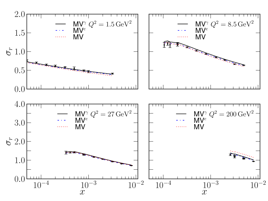
Figure 1: Reduced cross section $\sigma_{r}$ computed using the MV^γ, MV^e and MV model initial conditions for the dipole amplitude compared with combined HERA (H1 and ZEUS) data [8].

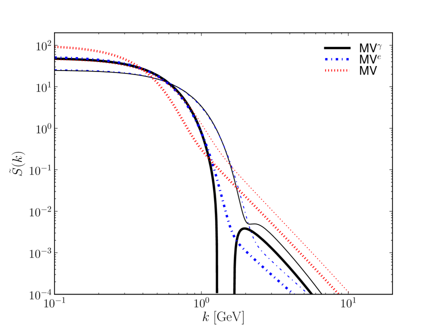
Figure 2: Two dimensional Fourier transform of $S(r)=1-{\mathcal{N}}(r)$ in fundamental (thick lines) and adjoint (thin lines) representations for MV^γ, MV^e and MV models.

Deep inelastic scattering provides a precision measurement of the proton structure. The H1 and ZEUS collaborations have measured the proton structure functions $F_{2}$ and $F_{L}$ and published very precise combined results for the reduced cross section $\sigma_{r}$ [8], which is a linear combination of the proton structure functions:

$$\sigma_{r}(y,x,Q^{2})=F_{2}(x,Q^{2})-\frac{y^{2}}{1+(1-y)^{2}}F_{L}(x,Q^{2}).$$ (1)

Here $y=Q^{2}/(sx)$ and $\sqrt{s}$ is the center of mass energy. The structure functions are related to the virtual photon-proton cross sections $\sigma_{T,L}^{\gamma^{*}p}$ for transverse (T) and longitudinal (L) photons that can, in the Color Glass Condensate framework, be computed as

$$\sigma_{T,L}^{\gamma^{*}p}(x,Q^{2})=2\sum_{f}\int\mathrm{d}z\int\mathrm{d}^{2}{\mathbf{b}_{T}}|\Psi_{T,L}^{\gamma^{*}\to f\bar{f}}|^{2}{\mathcal{N}}({\mathbf{b}_{T}},{\mathbf{r}_{T}},x).$$ (2)

Here $\Psi_{T,L}^{\gamma^{*}\to f\bar{f}}$ is the photon light cone wave function describing how the photon fluctuates to a quark-antiquark pair, computed from light cone QED [9]. The QCD dynamics is inside the function ${\mathcal{N}}({\mathbf{b}_{T}},{\mathbf{r}_{T}},x)$ which is the imaginary part of the scattering amplitude for the process where a dipole scatters off the color field of a hadron with impact parameter ${\mathbf{b}_{T}}$. It can not be computed perturbatively, but its energy (or equivalently Bjorken $x$) dependence satisfies the BK equation, for which we use the running coupling corrections derived in Ref. [10].

We assume here that the impact parameter dependence of the proton factorizes and one replaces

$$2\int\mathrm{d}^{2}{\mathbf{b}_{T}}\to\sigma_{0}.$$ (3)

Note that with the usual convention adopted here the factor 2 from the optical theorem is absorbed into the constant $\sigma_{0}$, thus the transverse area of the proton is now $\sigma_{0}/2$. The proton area could in principle be obtained from diffractive vector meson production, see discussion in Ref [7]. In this work, however, we consider $\sigma_{0}$ to be a fit parameter.

Model	$\chi^{2}/\text{d.o.f}$	$Q_{\mathrm{s0}}^{2}$ [GeV2]	$Q_{\mathrm{s}}^{2}$ [GeV2]	$\gamma$	$C^{2}$	$e_{c}$	$\sigma_{0}/2$ [mb]
MV	2.76	0.104	0.139	1	14.5	1	18.81
MVγ	1.17	0.165	0.245	1.135	6.35	1	16.45
MVe	1.15	0.060	0.238	1	7.2	18.9	16.36

Table 1: Parameters from fits to HERA reduced cross section data at $x<10^{-2}$ and $Q^{2}<50\,\mathrm{GeV}^{2}$ for different initial conditions. Also the corresponding initial saturation scales $Q_{\mathrm{s}}^{2}$ defined via equation ${\mathcal{N}}(r^{2}=2/Q_{\mathrm{s}}^{2})=1-e^{-1/2}$ are shown. The parameters for the MV^γ initial condition are obtained by the AAMQS collaboration [1].

As a non-perturbative input one needs also the dipole-proton amplitude at the initial $x=x_{0}$, for which we use a modified McLerran-Venugopalan model [11]:

$${\mathcal{N}}({\mathbf{r}_{T}})=1-\exp\left[-\frac{({\mathbf{r}_{T}}^{2}Q_{\mathrm{s0}}^{2})^{\gamma}}{4}\ln\left(\frac{1}{|{\mathbf{r}_{T}}|\Lambda_{\mathrm{QCD}}}+e_{c}\cdot e\right)\right],$$ (4)

where we have generalized the AAMQS [1] form by also allowing the constant inside the logarithm, which plays a role of an infrared cutoff, to be different from $e$. The other fit parameters are the anomalous dimension $\gamma$ and the initial saturation scale $Q_{\mathrm{s0}}^{2}$.

The BK equation with running coupling requires the strong coupling constant $\alpha_{\mathrm{s}}$ as a function of the transverse separation $r=|{\mathbf{r}_{T}}|$. In order to obtain a slow enough evolution to be compatible with the data (see discussion in Ref. [12]) we include, as in Ref. [1], an additional fit parameter $C^{2}$ such that (see also Ref. [13] for a discussion of the numerical value of $C^{2}$)

$$\alpha_{\mathrm{s}}(r)=\frac{12\pi}{(33-2N_{f})\log\left(\frac{4C^{2}}{r^{2}\Lambda_{\mathrm{QCD}}^{2}}\right)},$$ (5)

with $\Lambda_{\mathrm{QCD}}$ fixed to the value $0.241$ GeV.

The unknown parameters are obtained by performing a fit to small-$x$ DIS data. The first parametrization considered in this work, denoted by MV^γ, is obtained by setting $e_{c}\equiv 1$ in Eq. (4) but keeping the anomalous dimension $\gamma$ as a fit parameter. This is fitted by the AAMQS collaboration in Ref. [1], resulting in a very good $\chi^{2}/\text{d.o.f}\approx 1.17$. The obtained values for the parameters are listed in Table 1.

We fit the two other initial conditions for the dipole amplitude to the HERA reduced cross section data. First, we consider a parametrization, denoted here by MV^e, where we do not include anomalous dimension ($\gamma\equiv 1$) but let $e_{c}$ be a free fit parameter. The second model studied for comparison is the MV model without modifications, where $\gamma\equiv 1$ and $e_{c}\equiv 1$. The fit quality obtained using the MV^e initial condition is essentially as good as for the MV^γ model, with the best fit giving $\chi^{2}/\text{d.o.f}\approx 1.15$. The fit parameters are listed in Table 1. Viewed in momentum space this parametrization provides a smoother interpolation between the small-$k$ saturation region (where it resembles the Gaussian GBW form) and the power law at behavior high $k$. This is demonstrated in Fig. 2, where we show the Fourier-trasform of $S({\mathbf{r}_{T}})=1-{\mathcal{N}}({\mathbf{r}_{T}})$, which is proportional to the “dipole” gluon distribution.

The parameters obtained for the pure MV model, where $\gamma=1$ and $e_{c}=1$, are listed in Table 1. The fit quality is not as good as with the modified MV model, ($\chi^{2}/\text{d.o.f}\sim 2.8$), but as one can see from Fig. 2, the description of the small-$x$ DIS data is still reasonable.

3 Single inclusive hadron production in CGC

The gluon spectrum in heavy ion collisions can be obtained by solving the classical Yang-Mills equations of motion for the color fields. For $k_{T}\gtrsim Q_{\mathrm{s}}$ it has been shown numerically [14] that this solution is well approximated by the following $k_{T}$-factorized formula  [15]

$$\frac{\mathrm{d}\sigma}{\mathrm{d}y\mathrm{d}^{2}{\mathbf{k}_{T}}\mathrm{d}^{2}{\mathbf{b}_{T}}}=\frac{2\alpha_{\mathrm{s}}}{C_{\mathrm{F}}{\mathbf{k}_{T}}^{2}}\int\mathrm{d}^{2}{\mathbf{q}_{T}}\mathrm{d}^{2}{\mathbf{s}_{T}}\frac{\varphi_{p}({\mathbf{q}_{T}},{\mathbf{s}_{T}})}{{\mathbf{q}_{T}}^{2}}\frac{\varphi_{p}({\mathbf{k}_{T}}-{\mathbf{q}_{T}},{\mathbf{b}_{T}}-{\mathbf{s}_{T}})}{({\mathbf{k}_{T}}-{\mathbf{q}_{T}})^{2}}.$$ (6)

Here $\varphi_{p}$ is the dipole unintegrated gluon distribution (UGD) of the proton [16, 17, 18] and ${\mathbf{b}_{T}}$ is the impact parameter. For the proton we assume that the impact parameter dependence factorizes and

$$\varphi_{p}({\mathbf{k}_{T}})=\int\mathrm{d}^{2}{\mathbf{b}_{T}}\varphi_{p}({\mathbf{k}_{T}},{\mathbf{b}_{T}})=\frac{C_{\mathrm{F}}\sigma_{0}/2}{8\pi^{3}\alpha_{\mathrm{s}}}{\mathbf{k}_{T}}^{4}\tilde{S}^{p}({\mathbf{k}_{T}}).$$ (7)

Here $\tilde{S}^{p}(k)$ is the two dimensional Fourier transform of the dipole-proton scattering matrix $S^{p}(r)=1-{\mathcal{N}}^{p}_{A}(r)$, where ${\mathcal{N}}^{p}_{A}$ is the dipole-proton scattering amplitude in adjoint representation: ${\mathcal{N}}_{A}=2{\mathcal{N}}-{\mathcal{N}}^{2}$. For the proton DIS area $\sigma_{0}/2$ we use the value from the fits to DIS data, see Sec. 2.

Let us now consider a proton-proton collision. The cross section is obtained by integrating Eq. (6) over the impact parameter, which gives

$$\frac{\mathrm{d}\sigma}{\mathrm{d}y\mathrm{d}^{2}{\mathbf{k}_{T}}}=\frac{(\sigma_{0}/2)^{2}}{(2\pi)^{2}}\frac{C_{\mathrm{F}}}{2\pi^{2}{\mathbf{k}_{T}}^{2}\alpha_{\mathrm{s}}}\int\frac{\mathrm{d}^{2}{\mathbf{q}_{T}}}{(2\pi)^{2}}{\mathbf{q}_{T}}^{2}\tilde{S}^{p}({\mathbf{q}_{T}})({\mathbf{k}_{T}}-{\mathbf{q}_{T}})^{2}\tilde{S}^{p}({\mathbf{k}_{T}}-{\mathbf{q}_{T}}).$$ (8)

The invariant yield is defined as the production cross section divided by the total inelastic cross section $\sigma_{\text{inel}}$ and thus becomes

$$\frac{\mathrm{d}N}{\mathrm{d}y\mathrm{d}^{2}{\mathbf{k}_{T}}}=\frac{(\sigma_{0}/2)^{2}}{\sigma_{\text{inel}}}\frac{C_{\mathrm{F}}}{8\pi^{4}{\mathbf{k}_{T}}^{2}\alpha_{\mathrm{s}}}\int\frac{\mathrm{d}^{2}{\mathbf{q}_{T}}}{(2\pi)^{2}}{\mathbf{q}_{T}}^{2}\tilde{S}^{p}({\mathbf{q}_{T}})({\mathbf{k}_{T}}-{\mathbf{q}_{T}})^{2}\tilde{S}^{p}({\mathbf{k}_{T}}-{\mathbf{q}_{T}}).$$ (9)

Assuming that $|{\mathbf{k}_{T}}|$ is much larger than the saturation scale of one of the protons we obtain the hybrid formalism result

$$\frac{\mathrm{d}N}{\mathrm{d}y\mathrm{d}^{2}{\mathbf{k}_{T}}}=\frac{\sigma_{0}/2}{\sigma_{\text{inel}}}\frac{1}{(2\pi)^{2}}xg(x,{\mathbf{k}_{T}}^{2})\tilde{S}^{p}({\mathbf{k}_{T}}),$$ (10)

where

$$xg(x,{\mathbf{k}_{T}}^{2})=\int_{0}^{{\mathbf{k}_{T}}^{2}}\frac{\mathrm{d}{\mathbf{q}_{T}}^{2}}{{\mathbf{q}_{T}}^{2}}\varphi_{p}({\mathbf{q}_{T}})$$ (11)

is the integrated gluon distribution function. This can then be replaced by the conventional parton distribution function, for which we can use the CTEQ LO [19] pdf.

HERA measurements of diffractive vector meson electroproduction [20] indicate that the proton transverse area measured with a high virtuality probe is smaller than in soft interactions. In our case this shows up as a large difference in the numerical values of $\sigma_{0}/2$ and $\sigma_{\text{inel}}$, and leads to an energy dependent factor $\frac{\sigma_{0}/2}{\sigma_{\text{inel}}}\sim 0.2\dots 0.3$ in the particle yield (10), in contrast with the treatment often used in CGC calculations. Physically this corresponds to a two-component picture of the transverse structure of the nucleon (see also Ref. [21] for a very similar discussion). The small-$x$ gluons responsible for semihard particle production occupy a small area $\sim\sigma_{0}/2$ in the core of the nucleon. This core is surrounded by a nonperturbative edge that becomes larger with $\sqrt{s}$, but only participates in soft interactions that contribute to the large total inelastic cross section $\sigma_{\text{inel}}$. We will in Sec. 4 show that this separation between the two transverse areas brings much clarity to the extension of the calculation from protons to nuclei.

Now that also the normalization ($\sigma_{0}/2$) from HERA data is used in the calculation of the single inclusive spectrum, the result represents the actual LO CGC prediction for also the normalization of the spectrum. As is often the case for perturbative QCD, the LO result only agrees with data within a factor of $\sim 2$. We therefore multiply the resulting spectrum with a “$K$-factor” to bring it to the level of the experimental data. Now that the different areas $\sigma_{0}$ and $\sigma_{\text{inel}}$ are properly included, this factor has a more conventional interpretation of the expected effect of NLO corrections on the result; although it depends quite strongly on the fragmentation function.

In order to obtain a hadron spectrum from the parton spectrum we convolute the cross section with the DSS LO fragmentation function [22] and, when using the hybrid formalism, also add the light quark-initiated channel to the gluonic one in Eq. (10).

4 From proton to nucleus

Due to a lack of small-$x$ nuclear DIS data we can not perform a similar fit to nuclear targets than what is done with the proton. Instead we use the optical Glauber model to generalize our dipole-proton amplitude to dipole-nucleus scattering.

First we observe that the total dipole (size $r$)-proton cross section reads

$$\sigma_{\text{dip}}^{p}=\sigma_{0}{\mathcal{N}}^{p}(r).$$ (12)

In the dilute limit of very small dipoles the dipole-nucleus cross section should be just an incoherent sum of dipole-nucleon cross sections, i.e. $\sigma_{\text{dip}}^{A}=A\sigma_{\text{dip}}^{p}$. On the other hand for large dipoles we should have $\mathrm{d}\sigma_{\text{dip}}^{A}/\mathrm{d}^{2}{\mathbf{b}_{T}}\equiv 2{\mathcal{N}}^{A}({\mathbf{r}_{T}},{\mathbf{b}_{T}})\leq 2$. These requirements are satisfied with an exponentiated dipole-nucleus scattering amplitude

$${\mathcal{N}}^{A}({\mathbf{r}_{T}},{\mathbf{b}_{T}})=\left[1-\exp\left(-\frac{AT_{A}({\mathbf{b}_{T}})}{2}\sigma_{\text{dip}}^{p}\right)\right].$$ (13)

This form is an average of the dipole cross section over the fluctuating positions of the nucleons in the nucleus (see e.g. [23]), and thus incorporates in an analytical expression the fluctuations discussed e.g. in Ref. [24].

Using the form (13) directly in computing particle production is, however problematic. Because the forward $S$-matrix element $S=1-{\mathcal{N}}^{A}({\mathbf{r}_{T}},{\mathbf{b}_{T}})$ approaches a limiting value $\exp\left(-\frac{AT_{A}({\mathbf{b}_{T}})}{2}\sigma_{0}\right)\sim\exp\left(-A^{1/3}\right)$ and not exactly zero at large $r$, the dipole gluon distribution develops unphysical oscillations as a function of $k$. We therefore expand the proton-dipole cross section in Eq. (13) and use the approximation

$$\sigma_{\text{dip}}^{p}=\sigma_{0}{\mathcal{N}}^{p}({\mathbf{r}_{T}})\approx\sigma_{0}\frac{({\mathbf{r}_{T}}^{2}Q_{\mathrm{s0}}^{2})^{\gamma}}{4}\ln\left(\frac{1}{|{\mathbf{r}_{T}}|\Lambda_{\mathrm{QCD}}}+e_{c}\cdot e\right)$$ (14)

in the exponent of Eq. (13). The dipole-nucleus amplitude is then obtained by solving the rcBK evolution equation with an initial condition

$${\mathcal{N}}^{A}({\mathbf{r}_{T}},{\mathbf{b}_{T}})=1-\exp\left[-AT_{A}({\mathbf{b}_{T}})\frac{\sigma_{0}}{2}\frac{({\mathbf{r}_{T}}^{2}Q_{\mathrm{s0}}^{2})^{\gamma}}{4}\ln\left(\frac{1}{|{\mathbf{r}_{T}}|\Lambda_{\mathrm{QCD}}}+e_{c}\cdot e\right)\right].$$ (15)

We emphasize that besides the Woods-Saxon nuclear density $T_{A}({\mathbf{b}_{T}})$, all the parameters in this expression result from the fit to HERA data. The “optical Glauber” initial condition (15) also brings to evidence the advantage of the MV^e parametrization, which achieves a good fit to HERA data while imposing $\gamma=1$. In contrast to the MV^γ fit, this functional form avoids the ambiguity encountered in e.g. Ref. [24] of whether the factor $AT_{A}({\mathbf{b}_{T}})\sigma_{0}/2$ should be replaced by $(AT_{A}({\mathbf{b}_{T}})\sigma_{0}/2)^{\gamma}$ to achieve a natural scaling of $Q_{\mathrm{s}}^{2}$ with the nuclear thickness.

The fully impact parameter dependent BK equation develops unphysical Coulomb tails which would need an additional screening mechanism at the confinement scale (see e.g. [25]). We therefore solve the scattering amplitudes for each ${\mathbf{b}_{T}}$ independently. Due to the rapid increase of the scattering amplitude at low densities (large $|{\mathbf{b}_{T}}|$) this effectively causes the nucleus to grow rapidly on the edges at large energies. We do not consider this parametrization to be reliable at large $|{\mathbf{b}_{T}}|$, and when computing particle production at peripheral collisions we assume that $R_{pA}=1$ when the saturation scale is below the proton saturation scale, see dicussion in Ref. [6].

When computing proton-nucleus cross sections we compute convolutions of the nuclear and the proton unintegrated gluon distributions. In terms of the dipole amplitudes the $k_{T}$ factorization formula now reads

$$\frac{\mathrm{d}N({\mathbf{b}_{T}})}{\mathrm{d}y\mathrm{d}^{2}{\mathbf{k}_{T}}}=\frac{\sigma_{0}/2}{(2\pi)^{2}}\frac{C_{\mathrm{F}}}{2\pi^{2}{\mathbf{k}_{T}}^{2}\alpha_{\mathrm{s}}}\int\frac{\mathrm{d}^{2}{\mathbf{q}_{T}}}{(2\pi)^{2}}{\mathbf{q}_{T}}^{2}\tilde{S}^{p}({\mathbf{q}_{T}})({\mathbf{k}_{T}}-{\mathbf{q}_{T}})^{2}\tilde{S}^{A}({\mathbf{k}_{T}}-{\mathbf{q}_{T}}),$$ (16)

where $\tilde{S}^{p}$ and $\tilde{S}^{A}$ are Fourier transforms of the dipole-proton and dipole-nucleus scattering matrices, respectively. Assuming moreover that the transverse momentum of the produced parton is much larger than the proton saturation scale we get the hybrid formalism result

$$\frac{\mathrm{d}N({\mathbf{b}_{T}})}{\mathrm{d}y\mathrm{d}^{2}{\mathbf{k}_{T}}}=\frac{1}{(2\pi)^{2}}xg(x,{\mathbf{k}_{T}}^{2})\tilde{S}^{A}({\mathbf{k}_{T}}).$$ (17)

Notice that, in contrast to Eq. (10), in this case we do not get a factor $(\sigma_{0}/2)/\sigma_{\text{inel}}$ in the yield. One can then analytically show that this parametrization yields $R_{pA}\to 1$ at midrapidity and at large transverse momenta [6] at all $\sqrt{s}$, even as $\sigma_{\text{inel}}$ and thus $N_{\text{bin}}$ are changing with $\sqrt{s}$ while the initial saturation scale $Q_{\mathrm{s0}}$ is not.

In proton-nucleus collisions it is not possible to determine the impact parameter by measuring the total multiplicity as well as in heavy ion collisions, due to the large multiplicity fluctuations for a fixed impact parameter. The first LHC proton-lead results are divided into centrality classes based on the multiplicity or energy deposit in forward calorimeters. This is a difficult quantity to handle theoretically, so we assume that we can obtain reasonable estimates for different centrality classes by using a standard optical Glauber model. This difference should be kept in mind when comparing our calculations with the corresponding LHC results.

5 Results

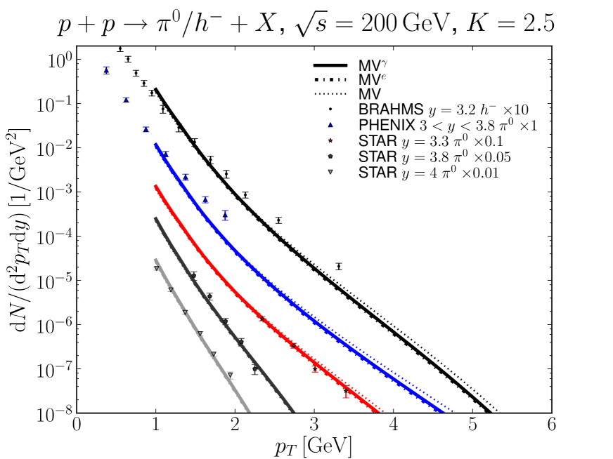
Figure 3: Single inclusive $\pi^{0}$ and negative hadron production computed using MV, MV^e and MV^γ initial conditions compared with RHIC data from STAR [26], PHENIX [27] and BRAHMS [28] collaborations.

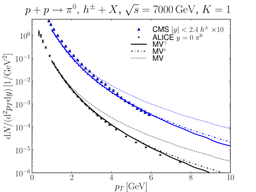
Figure 4: Single inclusive $\pi^{0}$ production computed using MV, MV^γ and MV^e initial conditions at $\sqrt{s}=7000$ GeV compared with ALICE $\pi^{0}$ [29] and CMS charged hadron data [30].

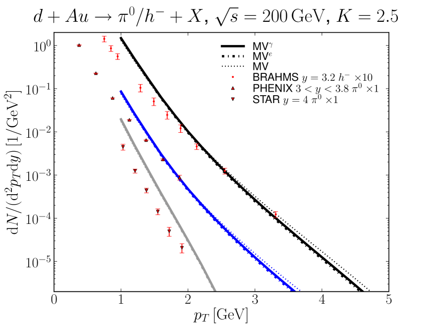
Figure 5: Single inclusive $\pi^{0}$ and negative hadron production at $\sqrt{s}=200$ GeV d+Au collisions compared with BRAHMS [28], STAR [26] and PHENIX [31] data.

Figure 6: Single inclusive charged hadron production in minimum bias p+Pb collisions at $\sqrt{s}=5020$ GeV computed using the $k_{T}$ factorization and compared with ALICE data [32].

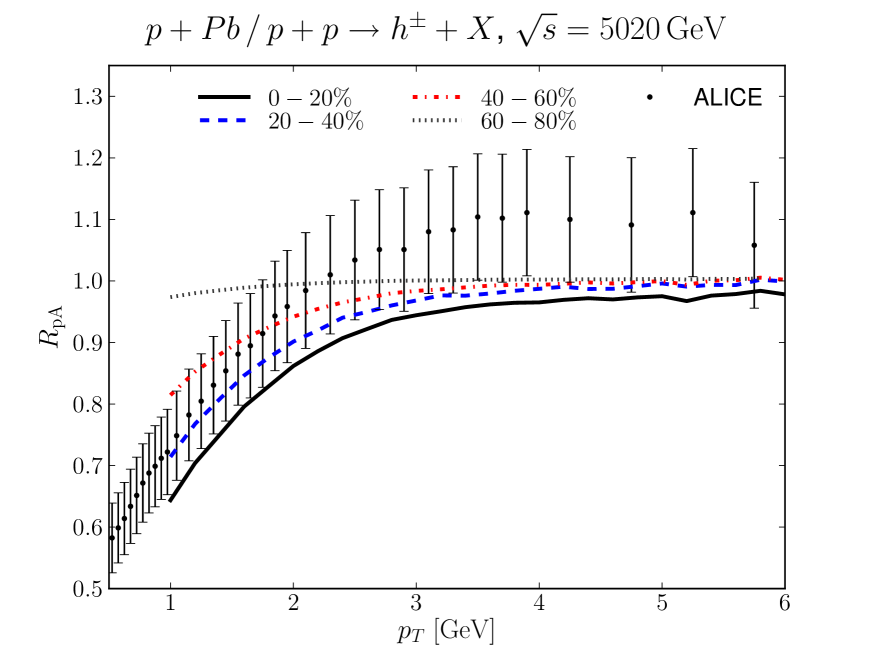
Figure 7: Centrality dependence of the nuclear modification factor $R_{pA}$ at $\sqrt{s}=5020$ GeV p+Pb collisions compared with the minimum bias ALICE data [32].

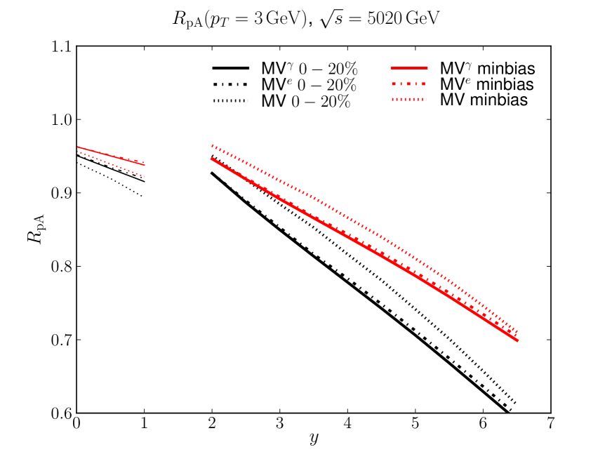
Figure 8: Rapidity dependence of the nuclear modification factor $R_{pA}$ for $3$ GeV neutral pion production at most central and minimum bias collisions.

In Fig. 4 we show the single inclusive $\pi^{0}$ and negative hadron yields computed using the hybrid formalism at $\sqrt{s}=200$ GeV and compare with the experimental data from RHIC [26, 27, 28]. As an initial condition for the BK evolution we use MV, MV^γ and MV^e fits. We recall that all fits, especially MV^γ and MV^e, give a good description of the HERA DIS data (see Fig. 2). We observe that all initial conditions yield very similar particle spectra, and especially the STAR $\pi^{0}$ spectra work very well, using $K=2.5$. The agreement with BRAHMS and PHENIX data is still reasonably good even though the $p_{T}$ slope is not exactly correct.

The midrapidity single inclusive $\pi^{0}$ and charged hadron yields at $\sqrt{s}=7000$ GeV computed using $k_{T}$-factorization and compared with ALICE [29] and CMS [30] data are shown in Fig. 4. Both MV^γ and MV^e models describe the data well without any additional $K$ factor. The pure MV model gives a too hard spectrum.

We have also tested that evaluating the parton distribution function or the fragmentation function at NLO instead of LO accuracy, using a different fragmentation function or using the hybrid formalism instead of the $k_{T}$-factorization does not significantly affect the $p_{T}$ slope of the single inclusive spectrum. On the other hand the absolute normalization depends quite strongly (up to a factor $\sim 4$) on these choices.

Let us then discuss proton-nucleus and deuteron-nucleus collisions. In Fig. 6 we present the single inclusive $\pi^{0}$ and negative charged hadron production yields in minimum bias deuteron-nucleus collisions at forward rapidities computed using the hybrid formalism and compared with the RHIC data [28, 26, 31]. We use here the same $K$ factor $K=2.5$ that was required to obtain correct normalization with the RHIC pp data. The $p_{T}$ slopes agree roughly with the data, whereas the absolute normalization differs slightly. In Fig. 6 we show the single inclusive charged hadron yield in proton-lead collisions compared with the ALICE data [32]. The conclusion is very similar as for proton-proton collisions (see Fig. 4): the pure MV model gives a wrong $p_{T}$ slope when comparing with the LHC data, but both MV^γ and MV^e models describe the data well.

The centrality dependence of the midrapidity $R_{pA}$ is shown in Fig. 8. Here we only compute results using the MV^e initial condition as $R_{pA}$ depends weakly on the initial condition. The centrality dependence is relatively weak, the results start to differ only at most peripheral classes. Notice that in our calculation we set explicitly $R_{pA}=1$ at centralities $\gtrsim 70\%$, see discussion in Sec. 4. The minimum bias result, which is obtained by averaging over the centrality classes, agrees with the ALICE data.

In order to further demonstrate the evolution speed of the nuclear modification factor we plot $R_{pA}({\mathbf{p}_{T}}=3\,\mathrm{GeV})$ for neutral pion production at LHC energies in Fig. 8 in central and minimum bias collisions. We compute $R_{pA}$ close to midrapidity using $k_{T}$-factorization and at forward rapidities using the hybrid formalism. Thus the obtained curve is not exactly continuous. The evolution speed close to midrapidity (where $k_{T}$-factorization should be valid) is slightly slower than at more forward rapidities where the hybrid formalism is more reliable. The MV model initial condition gives a slightly different result than the MV^γ and MV^e models, and all dipole models give basically the same evolution speed. Thus $R_{pA}$ is not sensitive to the details of the initial dipole amplitude, and the evolution speed of $R_{pA}$ is driven by the BK evolution. The centrality and especially rapidity evolution speed is significantly faster than in an NLO pQCD calculation using the EPS09s nuclear parton distribution functions [34, 35].

6 Conclusions

Taking only input from electron-proton deep inelastic scattering and standard nuclear geometry we compute single inclusive hadron production in proton-proton and proton-nucleus collisions from the Color Glass Condensate framework. We find that the MV model initial condition must be modified in order to obtain good description of the LHC single inclusive spectra. We have shown that instead of introducing an anomalous dimension one can also take the infrared cutoff in the MV model to be a fit parameter.

We obtain a good description of the available proton-nucleus and deuteron-nucleus data and get exactly $R_{pA}\to 1$ at large ${\mathbf{p}_{T}}$ which is a natural requirement and in agreement with the available ALICE data, and follows directly from our consistent treatment of the difference between the proton transverse areas. We present predictions for future forward $R_{pA}$ measurements. Especially we find that the rapidity evolution of the $R_{pA}$ at fixed ${\mathbf{p}_{T}}$ is a generic prediction of the CGC, given by the BK equation.

References

- [1] J. L. Albacete, N. Armesto, J. G. Milhano, P. Quiroga-Arias and C. A. Salgado, Eur. Phys. J. C71, 1705 (2011), [arXiv:1012.4408 [hep-ph]].
- [2] T. Lappi and H. Mäntysaari, Nucl. Phys. A908 (2013), [arXiv:1209.2853 [hep-ph]].
- [3] J. L. Albacete and C. Marquet, Phys. Rev. Lett. 105, 162301 (2010), [arXiv:1005.4065 [hep-ph]].
- [4] K. Dusling and R. Venugopalan, Phys. Rev. D87, 094034 (2013), [arXiv:1302.7018 [hep-ph]].
- [5] H. Kowalski, L. Motyka and G. Watt, Phys. Rev. D74, 074016 (2006), [arXiv:hep-ph/0606272].
- [6] T. Lappi and H. Mäntysaari, Phys. Rev. C87, 032201 (2013), [arXiv:1301.4095 [hep-ph]].
- [7] T. Lappi and H. Mäntysaari, arXiv:1309.6963 [hep-ph].
- [8] H1 and ZEUS, F. Aaron et al., JHEP 1001, 109 (2010), [arXiv:0911.0884 [hep-ex]].
- [9] Y. V. Kovchegov and E. Levin, Quantum chromodynamics at high energy (Cambridge University Press, 2012).
- [10] I. Balitsky, Phys. Rev. D75, 014001 (2007), [arXiv:hep-ph/0609105 [hep-ph]].
- [11] L. D. McLerran and R. Venugopalan, Phys. Rev. D49, 2233 (1994), [arXiv:hep-ph/9309289].
- [12] J. Kuokkanen, K. Rummukainen and H. Weigert, Nucl. Phys. A875, 29 (2012), [arXiv:1108.1867 [hep-ph]].
- [13] T. Lappi and H. Mäntysaari, Eur. Phys. J. C73, 2307 (2013), [arXiv:1212.4825 [hep-ph]].
- [14] J. P. Blaizot, T. Lappi and Y. Mehtar-Tani, Nucl. Phys. A846, 63 (2010), [arXiv:1005.0955 [hep-ph]].
- [15] Y. V. Kovchegov and K. Tuchin, Phys. Rev. D65, 074026 (2002), [arXiv:hep-ph/0111362 [hep-ph]].
- [16] D. Kharzeev, Y. V. Kovchegov and K. Tuchin, Phys. Rev. D68, 094013 (2003), [arXiv:hep-ph/0307037 [hep-ph]].
- [17] J. P. Blaizot, F. Gelis and R. Venugopalan, Nucl. Phys. A743, 13 (2004), [arXiv:hep-ph/0402256 [hep-ph]].
- [18] F. Dominguez, C. Marquet, B.-W. Xiao and F. Yuan, Phys. Rev. D83, 105005 (2011), [arXiv:1101.0715 [hep-ph]].
- [19] J. Pumplin et al., JHEP 0207, 012 (2002), [arXiv:hep-ph/0201195 [hep-ph]].
- [20] H1, F. Aaron et al., JHEP 1005, 032 (2010), [arXiv:0910.5831 [hep-ex]].
- [21] L. Frankfurt, M. Strikman and C. Weiss, Phys. Rev. D83, 054012 (2011), [arXiv:1009.2559 [hep-ph]].
- [22] D. de Florian, R. Sassot and M. Stratmann, Phys.Rev. D75, 114010 (2007), [arXiv:hep-ph/0703242 [HEP-PH]].
- [23] H. Kowalski, T. Lappi and R. Venugopalan, Phys. Rev. Lett. 100, 022303 (2008), [arXiv:0705.3047 [hep-ph]].
- [24] J. L. Albacete, A. Dumitru, H. Fujii and Y. Nara, Nucl. Phys. A897, 1 (2013), [arXiv:1209.2001 [hep-ph]].
- [25] K. J. Golec-Biernat and A. Stasto, Nucl. Phys. B668, 345 (2003), [arXiv:hep-ph/0306279 [hep-ph]].
- [26] STAR, J. Adams et al., Phys. Rev. Lett. 97, 152302 (2006), [arXiv:nucl-ex/0602011 [nucl-ex]].
- [27] PHENIX, A. Adare et al., Phys. Rev. Lett. 107, 172301 (2011), [arXiv:1105.5112 [nucl-ex]].
- [28] BRAHMS, I. Arsene et al., Phys. Rev. Lett. 93, 242303 (2004), [arXiv:nucl-ex/0403005 [nucl-ex]].
- [29] ALICE, B. Abelev et al., Phys. Lett. B717, 162 (2012), [arXiv:1205.5724 [hep-ex]].
- [30] CMS, V. Khachatryan et al., Phys. Rev. Lett. 105, 022002 (2010), [arXiv:1005.3299 [hep-ex]].
- [31] B. A. Meredith, A Study of Nuclear Effects using Forward-Rapidity Hadron Production and Di-Hadron Angular Correlations in GeV d+Au and p+p Collisions with the PHENIX Detector at RHIC (Ph.D. thesis at University of Illinois at Urbana-Champaign, 2011).
- [32] ALICE, B. Abelev et al., Phys. Rev. Lett. 110, 082302 (2013), [arXiv:1210.4520 [nucl-ex]].
- [33] D. d’Enterria, K. J. Eskola, I. Helenius and H. Paukkunen, arXiv:1311.1415 [hep-ph].
- [34] I. Helenius, K. J. Eskola, H. Honkanen and C. A. Salgado, JHEP 1207, 073 (2012), [arXiv:1205.5359 [hep-ph]].
- [35] I. Helenius, Private communication.