Assessment of mortgage default risk via Bayesian state space models

Abstract

Managing risk at the aggregate level is crucial for banks and financial institutions as required by the Basel III framework. In this paper, we introduce discrete time Bayesian state space models with Poisson measurements to model aggregate mortgage default rate. We discuss parameter updating, filtering, smoothing, forecasting and estimation using Markov chain Monte Carlo methods. In addition, we investigate the dynamic behavior of the default rate and the effects of macroeconomic variables. We illustrate the use of the proposed models using actual U.S. residential mortgage data and discuss insights gained from Bayesian analysis.

, and t1Supported by the NSF Grant DMS-09-1516 with George Washington University.

1 Introduction

Given the large size of outstanding residential mortgage loans in the U.S., a healthy mortgage market is important for stability of the financial markets and the whole economy. Due to its significant costs upon mortgage borrowers, lenders, insurers and investors of mortgage backed securities, management of mortgage default risk is one of the primary concerns for the policy makers and financial institutions.

Most commonly used measures of mortgage default risk are delinquency and foreclosure rates of mortgage loans. They provide a general description of how the mortgage market performs, compared to the macro economy. According to Gilberto and Houston (1989), mortgage default is legally defined as the transfer of property ownership from the borrower to the lender. The majority of researchers who focus on modeling of default risk define mortgage default as being delinquent in a mortgage payment for 90 days as discussed in Ambrose and Capone (1998). In this paper we use the latter definition to distinguish default from foreclosure.

Most of the work in the mortgage default risk literature has focused mainly on the individual default behavior of borrowers, and the effects of mortgage loan, property, borrower and economic characteristics on default risk. Quercia and Stegman (1992) provide a detailed literature review of research in mortgage default risk until 1992. More recent developments can be found in Leece (2004). There are two dominant classes of models in the literature. The first class of models is based on the ruthless default assumption and is option theoretic where the mortgage value, prepayment and default options are determined via stochastic behavior of prices and interest rates as in Kau et al. (1990). The second class is based on the hazard rate models where time to mortgage default is a random variable with hazard rate as a function of individual borrower and loan characteristics as studied by Lambrecht, Perraudin and Satchell (1997, 2003) and Soyer and Xu (2010). Both classes of models are based on the behavior of individual mortgages. But studying the default behavior at the aggregate level is also of interest to financial institutions and policy makers to be able to predict default rates and to develop appropriate mitigation instruments. As pointed out by Taufer (2007), managing risk at the aggregate level is crucial for banks and financial institutions as required by the Basel III framework which encourages banks to identify and manage present and future risks. Taufer (2007) models the probability of default at the aggregate level for two default classes, all-corporate and speculative-grades in U.S. as a stochastic process.

Modeling aggregate default rates requires consideration of several issues. First, it is important to identify the effect of macroeconomic variables on the aggregate default rate. This is pointed out by Taufer (2007) but is not considered in his model. Another issue to assess is if the aggregate default rate exhibits a dynamic behavior. In modeling individual default rates, Soyer and Xu (2010) point out that default rates are nonmonotonic. More specifically, the authors report that default rates are typically first increasing and then decreasing over the duration of the mortgage. It is not unreasonable to expect that the aggregate default rate will also follow such a dynamic behavior. Third, as noted by Kiefer (2011), it is not uncommon to have correlated defaults over time. Thus, it is desirable for models to capture such correlations.

In this paper, we present a discrete time Bayesian state-space model for Poisson counts to address the above issues. The proposed model enables us to describe the dynamic behavior of aggregate mortgage default rates over time and assumes a Markovian structure to describe the correlated default rates. This Markovian structure enables us to capture correlations between the number of defaults over time and provides an alternate way of modeling time-series of counts. Since the Markovian structure is assumed for the parameter, that is, for the default rate, our model can be classified as a parameter driven Markov model using the terminology of Cox (1981). We introduce an extension of the model by modulating the default rate by considering the effect of covariates describing the economic environment. This model can be considered a discrete time version of a modulated Poisson process model of Cox (1972). This class of models and their Bayesian analysis have not been considered in the literature before. To the best of our knowledge, only a few studies consider Bayesian methods in modeling mortgage default risk in the literature. Herzog (1988) introduces basic Bayesian concepts and Popova, Popova and George (2008) apply Bayesian methods to forecast mortgage prepayment rates. More recently, Kiefer (2010) introduces the incorporation of expert knowledge in estimating default rates from a Bayesian point of view, details a binomial model with dependent defaults and discusses implications of such models on risk management. As noted by Kiefer (2011), the Bayesian approach provides a coherent framework to combine data with prior information and enables us to make inferences using probabilistic reasoning. As will be discussed in our illustrations, additional insights are gained from the Bayesian analysis.

A summary of our paper is as follows: In Section 2 we introduce a Bayesian state space model for the monthly default counts for a given mortgage pool. Section 3 is dedicated to the development of a discrete time Bayesian state space model with covariates. We discuss the Bayesian analysis of the models in Section 4 using Markov chain Monte Carlo methods. An illustration of the proposed models is presented in Section 5 using real default count data for different mortgage pools where we discuss both in and out of sample fit issues for our models and compare them with the Bayesian Poisson regression which we use as a benchmark. Finally, in Section 6 we conclude with a summary of our findings and suggestions for future work.

2 A dynamic model for number of defaults

We first introduce a discrete time Bayesian model with Poisson observations and a default rate that evolves over time according to a Markov process. This model does not take into account the effects of covariates on the default rate of a given mortgage pool. Smith and Miller (1986) consider a similar state space model for exponential measurements which was used by Morali and Soyer (2003) in the context of software reliability.

Let $N_{t}$ be the number of defaults of a given mortgage pool during the month $t$ and $\theta_{t}$ be its default rate for $t=1,\ldots,T$. Given $\theta_{t}$, we assume that the number of defaults during the month $t$ is described by a discrete time nonhomogeneous Poisson process,

$$(N_{t}|\theta_{t})\sim\operatorname{Pois}(\theta_{t}).$$ (1)

In (1) it is assumed that given the default rate $\theta_{t}$, the default counts ${N_{t}}$s are conditionally independent. Also, (1) acts as an observation equation for discrete time.

For the state evolution equation of $\theta_{t}$’s, we assume that consecutive default rates exhibit a Markovian behavior similar to that considered by Taufer (2007) at the aggregate level. The Markovian evolution of default rates over time is described by

$$\theta_{t}=\frac{\theta_{t-1}}{\gamma}\varepsilon_{t},$$ (2)

where $(\varepsilon_{t}|N^{(t-1)})\sim\operatorname{Beta}[\gamma a_{t-1},(1-\gamma)a_{t-1}],a_{t-1}>0,0<\gamma<1$, and$N^{(t-1)}=\{N_{1},\ldots,N_{t-1}\}$. Here, $\gamma$ acts like a discounting term between consecutive default rates. An evolution structure similar to (2) was considered by Uhlig (1997) in the context of modeling stochastic volatility. A similar setup for a general family of non-Gaussian models was introduced by Santos, Gamerman and Franco (2012). Our model can be obtained as a special case.

The state equation (2) implies a stochastic ordering between the default rates, $\theta_{t}<\frac{\theta_{t-1}}{\gamma}$. Therefore, it can be shown that

$$\bigl{(}\theta_{t}|\theta_{t-1},N^{(t-1)}\bigr{)}\sim\operatorname{Beta}\biggl{[}\gamma a_{t-1},(1-\gamma)a_{t-1};\biggl{(}0,\frac{\theta_{t-1}}{\gamma}\biggr{)}\biggr{]},$$ (3)

that is, a truncated Beta density. If one assumes that a priori $\theta_{0}$ follow a gamma density as

$$\bigl{(}\theta_{0}|N^{(0)}\bigr{)}\sim\operatorname{Gamma}(a_{0},b_{0}),$$ (4)

then one can develop an analytically tractable Bayesian analysis for the model. Following Smith and Miller (1986), as a result of (2) and (4) we can obtain

$$\bigl{(}\theta_{t-1}|N^{(t-1)}\bigr{)}\sim\operatorname{Gamma}(a_{t-1},b_{t-1}),$$ (5)

which can be shown by induction. Given the measurement equation (1), the state evolution equation (2) and the prior (4), the posterior default rates and one-step-ahead default count densities can be obtained analytically.

Predictive density for the default rate given default counts up to time $t-1$ is given by

$$\bigl{(}\theta_{t}|N^{(t-1)}\bigr{)}\sim\operatorname{Gamma}(\gamma a_{t-1},\gamma b_{t-1}).$$ (6)

It follows from the above that $E(\theta_{t}|N^{(t-1)})=E(\theta_{t-1}|N^{(t-1)})$ and$V(\theta_{t}|N^{(t-1)})=\frac{V(\theta_{t-1}|N^{(t-1)})}{\gamma}$. In other words, the model implies that as we move forward in time, the expected default rate stays the same but our uncertainty about the rate increases.

The posterior density of the default rate given default counts up to time $t$ is given by

$$\bigl{(}\theta_{t}|N^{(t)}\bigr{)}\sim\operatorname{Gamma}(a_{t},b_{t}),$$ (7)

where $a_{t}=\gamma a_{t-1}+N_{t}$ and $b_{t}=\gamma b_{t-1}+1$. The posterior density (7) is also known as the filtering distribution of the default rate.

Finally, one-month-ahead forecasting density of $N_{t}$ given the default counts up to month $t-1$ can be obtained to be a negative binomial density as

$$\bigl{(}N_{t}|N^{(t-1)}\bigr{)}\sim\operatorname{Negbin}(r_{t},p_{t}),$$ (8)

where $r_{t}=\gamma a_{t-1}$ and $p_{t}=\frac{\gamma b_{t-1}}{\gamma b_{t-1}+1}$. As summarized above, conditional on the discount factor $\gamma$, the updating of the default rate in light of new default information and one-month-ahead forecasting densities for default counts are all available analytically. Another attractive feature of the proposed model is that in addition to obtaining point estimates of the default counts and the default rates at each point in time, one can also obtain well-known probability distributions with easy to obtain statistical properties such as the mode, median, standard deviation and credibility intervals.

As noted by the associate editor, “as homeowners default or pay off their mortgages, the size of the effective pool of homeowners that could default changes.” Thus, knowing the original size of a given mortgage cohort and the number of people who prepay their mortgages might have been useful in our analysis. If such information is available, then it is possible to introduce a Poisson structure that can capture the behavior of the mortgage size and the prepayment counts over time by redefining $N_{t}$ as $N_{t}\sim\operatorname{Pois}(h_{t}\lambda_{t})$ and $P_{t}\sim\operatorname{Pois}(h_{t}\phi_{t})$, where $h_{t}$ is the mortgage size at time $t$ and $P_{t}$ is the number of prepaid mortgages at time $t$. Thus, we can keep track of the evolution of $h_{t}$ as $h_{t}=h_{t-1}-N_{t-1}-P_{t-1}$, where $\lambda_{t}$ and $\phi_{t}$ have Markovian evolutions similar to the one introduced in (2). Unfortunately, neither the size of the cohorts nor the prepayment counts were made available to us. In modeling the default risk at the aggregate level, the size of each cohort is very large as opposed to monthly default counts as pointed out by Kiefer (2010) with the default probability being very small. In our analysis of mortgage defaults since $h_{t}$ is not known to us, the default rate $\theta_{t}$ would be approximately equal to $h_{t}\lambda_{t}$.

3 Dynamic models with covariates

3.1 Dynamic model with static covariate coefficients

We next extend the model of Section 2 by considering the effects of covariates on the dynamic default rate. Let $N_{t}$ be the number of defaults of a given mortgage pool during the month $t$ and $\lambda_{t}$ be its default rate for $t=1,\ldots,T$. We assume that the default rate is given by

$$\lambda_{t}=\theta_{t}e^{\bolds{\beta}^{\prime}\mathbf{z}_{t}},$$ (9)

where $\mathbf{z}_{t}$ is the vector of the covariates and $\bolds{\beta}$ is the parameter vector. The covariate vector $\mathbf{z}_{t}$ may consist of economic variables as well as trend and seasonal components. Parameter $\theta_{t}$ acts like the baseline default rate which evolves over time. We also note that (9) is similar to a proportional hazards model. Given $\lambda_{t}$, we assume that the number of defaults during the month $t$ is described by a modulated nonhomogeneous Poisson process,

$$(N_{t}|\theta_{t},\bolds{\beta},\mathbf{z}_{t})\sim\operatorname{Pois}\bigl{(}\theta_{t}e^{\bolds{\beta}^{\prime}\mathbf{z}_{t}}\bigr{)}.$$ (10)

The modulated Poisson model (10) acts as an observation equation defined over discrete time. For the state evolution equation of the baseline failure rate, $\theta_{t}$, we assume the same structure as before given by (2). In addition, we assume that initially $(\theta_{0}|\bolds{\beta},\mathbf{z}_{t},N^{(0)})\sim\operatorname{Gamma}(a_{0},b_{0})$ and is independent of $\bolds{\beta}$. Thus, it can be shown that the conditional distribution of $(\theta_{t-1}|\bolds{\beta},\mathbf{z}_{t},N^{(t-1)})$ follows a gamma density as

$$\bigl{(}\theta_{t-1}|\bolds{\beta},\mathbf{z}_{t},N^{(t-1)}\bigr{)}\sim\operatorname{Gamma}(a_{t-1},b_{t-1}).$$ (11)

Therefore, the conditional posterior density of $\theta_{t}$ given $\bolds{\beta},\mathbf{z}_{t},N^{(t-1)}$ can be obtained via

$$\qquad p\bigl{(}\theta_{t}|\bolds{\beta},\mathbf{z}_{t},N^{(t-1)}\bigr{)}=\int^{\infty}_{\gamma\theta_{t}}p\bigl{(}\theta_{t}|\theta_{t-1},N^{(t-1)}\bigr{)}p\bigl{(}\theta_{t-1}|\bolds{\beta},\mathbf{z}_{t},N^{(t-1)}\bigr{)}\,d\theta_{t-1},$$ (12)

which reduces to a gamma density as

$$\bigl{(}\theta_{t}|\bolds{\beta},\mathbf{z}_{t},N^{(t-1)}\bigr{)}\sim\operatorname{Gamma}(\gamma a_{t-1},\gamma b_{t-1}).$$ (13)

Furthermore, the conditional posterior of $\theta_{t}$ given $\bolds{\beta},\mathbf{z}_{t},N^{(t)}$ can be obtained using (10) and (13) and the Bayes’ rule

$$p\bigl{(}\theta_{t}|\bolds{\beta},\mathbf{z}_{t},N^{(t)}\bigr{)}\propto p(N_{t}|\bolds{\beta},\mathbf{z}_{t},\theta_{t})p\bigl{(}\theta_{t}|\bolds{\beta},\mathbf{z}_{t},N^{(t-1)}\bigr{)}.$$ (14)

The above implies that

$$p\bigl{(}\theta_{t}|\bolds{\beta},\mathbf{z}_{t},N^{(t)}\bigr{)}\propto\bigl{(}\theta_{t}e^{\bolds{\beta}^{\prime}\mathbf{z}_{t}}\bigr{)}^{\gamma a_{t-1}+N_{t}-1}e^{-(\gamma b_{t-1}+1)(\theta_{t}e^{\bolds{\beta}^{\prime}\mathbf{z}_{t}})},$$

that is, the conditional distribution of the default rate at time $t$ is a gamma density given by

$$\bigl{(}\theta_{t}|\bolds{\beta},\mathbf{z}_{t},N^{(t)}\bigr{)}\sim\operatorname{Gamma}(a_{t},b_{t}),$$ (15)

where $a_{t}=\gamma a_{t-1}+N_{t}$ and $b_{t}=\gamma b_{t-1}+e^{\bolds{\beta}^{\prime}\mathbf{z}_{t}}$.

The one-step-ahead conditional predictive distribution of default counts at time $t$ given $\bolds{\beta},\mathbf{z}_{t}$ and $N^{(t-1)}$ can be obtained via

$$p\bigl{(}N_{t}|\bolds{\beta},\mathbf{z}_{t},N^{(t-1)}\bigr{)}=\int_{0}^{\infty}p(N_{t}|\bolds{\beta},\mathbf{z}_{t},\theta_{t})p\bigl{(}\theta_{t}|\bolds{\beta},\mathbf{z}_{t},N^{(t-1)}\bigr{)}\,d\theta_{t},$$ (16)

where $(N_{t}|\bolds{\beta},\mathbf{z}_{t},\theta_{t})\sim\operatorname{Pois}(\theta_{t}e^{\bolds{\beta}^{\prime}\mathbf{z}_{t}})$ and $(\theta_{t}|\bolds{\beta},\mathbf{z}_{t},N^{(t-1)})\sim\operatorname{Gamma}(\gamma a_{t-1},\break\gamma b_{t-1})$. Therefore,

$$p\bigl{(}N_{t}|\bolds{\beta},\mathbf{z}_{t},N^{(t-1)}\bigr{)}$$

(17)

$$\qquad=\pmatrix{{\gamma a_{t-1}+N_{t}-1}\vspace*{2pt}\cr{N_{t}}}\biggl{\{}\frac{\gamma b_{t-1}}{\gamma b_{t-1}+e^{\bolds{\beta}^{\prime}\mathbf{z}_{t}}}\biggr{\}}^{\gamma a_{t-1}}\biggl{\{}\frac{e^{\bolds{\beta}^{\prime}\mathbf{z_{t}}}}{\gamma b_{t-1}+e^{\bolds{\beta}^{\prime}\mathbf{z}_{t}}}\biggr{\}}^{N_{t}},$$

which is a negative binomial model denoted as

$$\bigl{(}N_{t}|N^{(t-1)},\bolds{\beta},\mathbf{z}_{t}\bigr{)}\sim\operatorname{Negbin}(r_{t},p_{t}),$$ (18)

where $r_{t}=\gamma a_{t-1}$ and $p_{t}=\frac{\gamma b_{t-1}}{\gamma b_{t-1}+e^{\bolds{\beta}^{\prime}\mathbf{z}_{t}}}$. The predictive density (18) implies that given the covariates and the default counts up to month $t-1$, forecasts for the month $t$ are a function of the observed default count in month $t-1$ adjusted by the corresponding covariates. The mean of $(N_{t}|N^{(t-1)},\bolds{\beta},\mathbf{z}_{t})$ can be computed via

$$E\bigl{(}N_{t}|N^{(t-1)},\bolds{\beta},\mathbf{z}_{t}\bigr{)}=\frac{a_{t-1}}{b_{t-1}}e^{\bolds{\beta}^{\prime}\mathbf{z}_{t}}.$$ (19)

Since the results previously presented are conditional on the parameter vector $\bolds{\beta}$ and the discount factor $\gamma$, we next discuss how to obtain the posterior distributions of $\bolds{\beta}$ and $\gamma$. Since these distributions cannot be obtained analytically, we will use Markov chain Monte Carlo (MCMC) methods to generate samples from these posterior distributions.

3.2 Dynamic model with dynamic covariate coefficients

A natural extension of the dynamic model with covariates is to let the regression coefficients vary over time. As pointed out by one of the reviewers, in volatile economic environments, macroeconomic variables might exhibit sudden ups and downs and being able to capture the effects of such changes will be of concern to institutions that are managing the mortgage loans. One way to take into account such changes is to allow a dynamic structure on the covariate coefficients. Following the same notation introduced previously, we assume that the number of defaults during the month $t$ is described by

$$(N_{t}|\theta_{t},\bolds{\beta}_{t},\mathbf{z}_{t})\sim\operatorname{Pois}\bigl{(}\theta_{t}e^{\bolds{\beta_{t}}^{\prime}\mathbf{z}_{t}}\bigr{)}.$$ (20)

In (20), $\bolds{\beta}_{t}$s are time varying coefficients and we assume the same structure on $\theta_{t}$ as in (2). The conditional updating of $\theta_{t}$s will be the same as introduced in Section 3 and their details will be omitted from the discussion to preserve space. Time evolution of the covariate coefficients is described by

$$\beta_{it}\sim N(\beta_{it-1},\tau_{i})\qquad\forall i,$$ (21)

where $i$ represents the covariate index, $\tau_{i}$ is the precision parameter for each $i$ and its prior is assumed to be

$$\tau_{i}\sim\operatorname{Gamma}(a_{\tau},b_{\tau})\qquad\forall i.$$ (22)

We use this extension in our numerical example in Section 5 to learn if dynamic nature of the covariate effects improves model fit and forecasting performance.

4 Bayesian analysis

Most of the parameter updating and forecasting for the dynamic model presented in Section 2 is available in closed form given that the discounting term $\gamma$ is known. Alternatively, one can assume an unknown $\gamma$ and use Bayesian analysis to carry out inference. Following the development of Section 3, the distributions obtained for the dynamic model with covariates are all conditional on $\bolds{\beta}$ and $\gamma$. Our objective is to obtain the posterior joint distribution of the model parameters given that we have observed all default counts up to time $t$, that is, $p(\theta_{1},\ldots,\theta_{t}|N^{(t)})$ for the dynamic model and $p(\theta_{1},\ldots,\theta_{t},\bolds{\beta}|N^{(t)})$ for the dynamic model with covariates, both of which can be used to infer mortgage default risk behavior of a given cohort. In addition, being able to obtain one-month-ahead predictive distributions of the default counts, $p(N_{t}|N^{(t-1)})$, will be of interest to institutions that are managing the loans.

4.1 Posterior inference

Since our goal is to obtain $p(\theta_{1},\ldots,\theta_{t},\bolds{\beta}|N^{(t)})$ which is not available in closed form, we can use a Gibbs sampler to generate samples from it. In order to do so, we need to be able to generate samples from the full conditional distributions of $p(\theta_{1},\ldots,\theta_{t}|\bolds{\beta},N^{(t)})$ and $p(\bolds{\beta}|\theta_{1},\ldots,\theta_{t},N^{(t)})$, none of which are available as known densities. Next, we discuss how to generate samples from these densities.

The conditional posterior distribution of $\bolds{\beta}$ given the default rates can be obtained by

$$p\bigl{(}\bolds{\beta}|\theta_{1},\ldots,\theta_{t},z_{t},N^{(t)}\bigr{)}\propto\prod_{i=1}^{t}\frac{\operatorname{exp}\{\theta_{i}e^{\bolds{\beta}^{\prime}\mathbf{z}_{i}}\}(\theta_{i}e^{\bolds{\beta}^{\prime}\mathbf{z}_{i}})^{N_{i}}}{N_{i}!}p(\bolds{\beta}),$$ (23)

where $p(\bolds{\beta})$ is the prior for $\bolds{\beta}$. Regardless of the prior selection for $\bolds{\beta}$, (23) will not be a known density. Therefore, we can use a random walk Metropolis–Hastings algorithm to be able to generate samples from $p(\bolds{\beta}|\theta_{1},\ldots,\theta_{t},z_{t},N^{(t)})$. Following Chib and Greenberg (1995), the steps in the Metropolis–Hastings algorithm can be summarized as follows: [1.]

Assume the starting points $\bolds{\beta}^{(0)}$ at $j=0$.

Repeat for $j>0$.

Generate $\bolds{\beta}^{*}$ from $q(\bolds{\beta}^{*}|\bolds{\beta}^{(j)})$ and $u$ from $U(0,1)$.

If $u\leq a(\bolds{\beta}^{(j)},\bolds{\beta}^{*})$ then set $\bolds{\beta}^{(j)}=\bolds{\beta}^{*}$; else set $\bolds{\beta}^{(j)}=\bolds{\beta}^{(j)}$ and $j=j+1$, where

$$a\bigl{(}\bolds{\beta}^{(j)},\bolds{\beta}^{*}\bigr{)}=\operatorname{min}\biggl{\{}1,\frac{\pi(\bolds{\beta}^{*})q(\bolds{\beta}^{(j)}|\bolds{\beta}^{*})}{\pi(\bolds{\beta}^{(j)})q(\bolds{\beta}^{*}|\bolds{\beta}^{(j)})}\biggr{\}}.$$ (24)

In (24), $\pi(\cdot)$ is given by (23), that is, the density we need to generate samples from, and $q(\cdot|\cdot)$ is the multivariate normal proposal density whose variance-covariance matrix is determined via $(-H)^{-1}$ with $H$ representing the approximate Hessian of $\pi(\cdot)$ evaluated at its mode; see Gelman et al. (1995). If we repeat the above a large number of times, then we obtain samples from $p(\bolds{\beta}|\theta_{1},\ldots,\theta_{t},z_{t},N^{(t)})$. Next, we discuss how one can generate samples from the other full conditional distribution, $p(\theta_{1},\ldots,\theta_{t}|\bolds{\beta},\mathbf{z}_{t},N^{(t)})$.

Due to the Markovian nature of the default rates, using the chain rule, we can rewrite the full conditional density, $p(\theta_{1},\ldots,\theta_{t}|\bolds{\beta},\mathbf{z}_{t},N^{(t)})$, as

$$p\bigl{(}\theta_{t}|\bolds{\beta},\mathbf{z}_{t},N^{(t)}\bigr{)}p\bigl{(}\theta_{t-1}|\theta_{t},\bolds{\beta},\mathbf{z}_{t},N^{(t-1)}\bigr{)}\cdots p\bigl{(}\theta_{1}|\theta_{2},\bolds{\beta},\mathbf{z}_{t},N^{(1)}\bigr{)}.$$ (25)

In (25), $p(\theta_{t}|\bolds{\beta},\mathbf{z}_{t},N^{(t)})$ is available from (15) and $p(\theta_{n-1}|\theta_{n},\bolds{\beta},\mathbf{z}_{t},N^{(n-1)})$ for any $n$ can be obtained as follows:

$$p\bigl{(}\theta_{n-1}|\theta_{n},\bolds{\beta},\mathbf{z}_{t},N^{(n-1)}\bigr{)}$$

(26)

$$\qquad\propto p\bigl{(}\theta_{n}|\theta_{n-1},\bolds{\beta},\mathbf{z}_{t},N^{(n-1)}\bigr{)}p\bigl{(}\theta_{n-1}|\bolds{\beta},\mathbf{z}_{t},N^{(n-1)}\bigr{)}.$$

It can be shown that $(\theta_{n-1}|\theta_{n},\bolds{\beta},\mathbf{z}_{t},N^{(n-1)})\sim\operatorname{Gamma}[(1-\gamma)a_{n-1},b_{n-1}]$, where $\gamma\theta_{n}<\theta_{n-1}<\infty$, that is, a truncated gamma density.

Therefore, given (25) and the posterior samples generated from the full conditional distribution of $\bolds{\beta}$, we can sample from $p(\theta_{1},\ldots,\theta_{t}|\bolds{\beta},\mathbf{z}_{t},N^{(t)})$ by sequentially simulating the individual default rates as follows: [1.]

Assume the starting points $\theta_{1}^{(0)},\ldots,\theta_{t}^{(0)}$ at $j=0$.

Repeat for $j>0$.

Using the generated $\bolds{\beta}^{(j)}$, sample $\theta^{(j)}_{t}$ from $(\theta_{t}|\bolds{\beta}^{(j)},\mathbf{z}_{t},N^{(t)})$.

Using the generated $\bolds{\beta}^{(j)}$, for each $n=t-1,\ldots,1$ generate $\theta^{(j)}_{n}$ from $(\theta_{n}|\theta^{(j)}_{n+1},\bolds{\beta},\mathbf{z}_{t},N^{(n)})$ where $\theta^{(j)}_{n+1}$ is the value generated in the previous step. If we repeat the above a large number of times, then we obtain samples from the joint full conditional distribution of default rates. The generation of $\theta^{(j)}_{n}$s in step 3 above is known as the forward filtering backward sampling algorithm; see Frühwirth-Schnatter (1994). Consequently, we can obtain samples from the joint density of the model parameters by iteratively sampling from $p(\bolds{\beta}|\theta_{1},\ldots,\theta_{t},z_{t},N^{(t)})$ and $p(\theta_{1},\ldots,\theta_{t}|\bolds{\beta},\mathbf{z}_{t},N^{(t)})$, namely, a full Gibbs sampler algorithm; see Smith and Gelfand (1992).

The FFBS algorithm as discussed above can also be used to generate samples from $p(\theta_{1},\ldots,\theta_{t}|N^{(t)})$ for the dynamic model without the use of the additional Gibbs sampler step for $\bolds{\beta}$. In addition, the above algorithm allows us to obtain a density estimate for $p(\theta_{t-k}|N^{(t)})$ for all $k\geq 1$ for both dynamic models which can be used for retrospective comparison of default rates among different mortgage pools. To the best of our knowledge, this type of approach has not been considered in the mortgage default risk literature.

4.2 Unknown discount parameter $\gamma$

Previously the discount factor $\gamma$ has been assumed to be known. If $\gamma$ were to be treated as an unknown quantity, then it is possible to obtain its Bayesian updating. Following the development of the dynamic model introduced in Section 2, the posterior distribution of $\gamma$ can be obtained by

$$p\bigl{(}\gamma|N^{(t)}\bigr{)}\propto\prod_{k=1}^{t}p\bigl{(}N_{k}|N^{(k-1)},\gamma\bigr{)}p(\gamma),$$ (27)

where $p(N_{k}|N^{(k-1)},\gamma)$ is the likelihood term which is given by (8) and $p(\gamma)$ is the prior for $\gamma$. Since (27) will not be a known density for any prior for $\gamma$, we need to sample from the posterior distribution of $\gamma$ using MCMC. As an alternative, a discrete prior over $(0,1)$ can be considered which can numerically be summed out from (27).

For the dynamic model with covariates detailed in Section 3, one can generate samples from the posterior joint distribution of $\gamma$ and $\bolds{\beta}$ from the following:

$$p\bigl{(}\gamma,\bolds{\beta}|N^{(t)},\mathbf{z}_{t}\bigr{)}\propto p(N_{1},\ldots,N_{t}|\mathbf{z}_{t},\gamma,\bolds{\beta})p(\gamma,\bolds{\beta}),$$ (28)

where $p(\gamma,\bolds{\beta})=p(\gamma)p(\bolds{\beta})$ when $\gamma$ and $\bolds{\beta}$ are assumed to be independent a priori and the likelihood term, $p(N_{1},\ldots,N_{t}|\mathbf{z}_{t},\gamma,\bolds{\beta})$, can be obtained as

$$\qquad p(N_{1},\ldots,N_{t}|\mathbf{z}_{t},\gamma,\bolds{\beta})=L\bigl{(}\gamma,\bolds{\beta};\mathbf{z}_{t},N^{(t)}\bigr{)}=\prod_{k=1}^{t}p\bigl{(}N_{k}|N^{(k-1)},\mathbf{z}_{t},\bolds{\beta},\gamma\bigr{)},$$ (29)

where $p(N_{k}|N^{(k-1)},\mathbf{z}_{t},\bolds{\beta},\gamma)$ is given by (18). The fact that (29) is free of $\theta_{t}$s facilitates the posterior generation. Since (28) will not be available in closed form for any prior of $\gamma$ and $\bolds{\beta}$, one can use a Metropolis–Hastings algorithm to generate samples from the joint posterior density as presented in Section 3.1. This approach can also be used to estimate $p(\gamma,\bolds{\beta}_{t}|\tau_{1},\ldots,\tau_{2},N^{(t)},\mathbf{z}_{t})$ for the model with dynamic covariates of Section 4.1. Thus, a Gibbs sampler can be used to obtain samples from the full joint distribution of all model parameters by iteratively generating samples between $p(\gamma,\bolds{\beta}_{t}|\tau_{1},\ldots,\tau_{2},N^{(t)},\mathbf{z}_{t})$ and $p(\tau_{i}|\bolds{\beta}_{t},\gamma,N^{(t)},\mathbf{z}_{t})$’s.

In addition, $p(\theta_{1},\ldots,\theta_{t}|N^{(t)},\mathbf{z}_{t},\bolds{\beta},\gamma)$, the conditional joint distribution of the default rates, can be obtained using the FFBS algorithm as presented in Section 4.1. Thus, the joint smoothing distribution of the default rates can be computed by

$$\qquad p\bigl{(}\theta_{1},\ldots,\theta_{t}|N^{(t)}\bigr{)}=\int\!\!\int p\bigl{(}\theta_{1},\ldots,\theta_{t}|N^{(t)},\mathbf{z}_{t},\bolds{\beta},\gamma\bigr{)}p\bigl{(}\gamma,\bolds{\beta}|N^{(t)}\bigr{)}\,d\gamma\,d\bolds{\beta},$$ (30)

where only samples from $p(\gamma,\bolds{\beta}|N^{(t)})$ will be available. Therefore, the above can be approximated as a Monte Carlo average via

$$p\bigl{(}\theta_{1},\ldots,\theta_{t}|N^{(t)}\bigr{)}\approx\frac{1}{S}\sum_{j=1}^{S}p\bigl{(}\theta_{1},\ldots,\theta_{t}|N^{(t)},\mathbf{z}_{t},\bolds{\beta}^{(j)},\gamma^{(j)}\bigr{)},$$ (31)

where $S$ is the number of samples, and $(\bolds{\beta}^{(j)},\gamma^{(j)})$ are the generated sample pairs.

4.3 One-month-ahead forecasting

In order to obtain one-month-ahead forecast distributions from the dynamic model with covariates, the following can be used:

$$p\bigl{(}N_{t}|N^{(t-1)},\mathbf{z}_{t}\bigr{)}=\int\!\!\int p\bigl{(}N_{t}|N^{(t-1)},\mathbf{z}_{t},\bolds{\beta},\gamma\bigr{)}p\bigl{(}\gamma,\bolds{\beta}|N^{(t)}\bigr{)}\,d\bolds{\beta}\,d\gamma.$$ (32)

Since only samples from $p(\gamma,\bolds{\beta}|N^{(t)})$ will be available, the above can be approximated by

$$p\bigl{(}N_{t}|N^{(t-1)},\mathbf{z}_{t}\bigr{)}\approx\frac{1}{S}\sum_{j=1}^{S}p\bigl{(}N_{t}|N^{(t-1)},\mathbf{z}_{t},\bolds{\beta}^{(j)},\gamma^{(j)}\bigr{)}.$$ (33)

Similarly, (33) can be computed for the dynamic model of Section 2 without any covariates and the dynamic model with dynamic covariates of Section 4.1.

4.4 Model comparison

In order to compare the fit of the proposed models to data, we consider two sets of measures that are used with sampling based methods, the Bayes factor with the harmonic mean estimator and the pseudo Bayes factor with the conditional predictive ordinate. In what follows, we briefly summarize both methods whose implementations are discussed in our numerical example.

4.4.1 Bayes factor-harmonic mean estimator

The first fit measure is the Bayes factor approximation of models with MCMC steps; we refer to this measure as the Bayes factor-harmonic mean estimator which has been discussed by Gelfand, Dey and Chang (1992) and Kass and Raftery (1995). The harmonic mean estimator of the predictive likelihood for a given model can be obtained as

$$p\bigl{(}N^{(t)}\bigr{)}=\Biggl{\{}\frac{1}{S}\sum_{j=1}^{S}p\bigl{(}N^{(t)}|\bolds{\Theta}^{(j)}\bigr{)}^{-1}\Biggr{\}}^{-1},$$ (34)

where $S$ is the number of iterations and $\bolds{\Theta}^{(j)}$ is the $j$th generated posterior sample. For the proposed models, (34) can be computed via

$$p\bigl{(}N^{(t)}\bigr{)}=\Biggl{\{}\frac{1}{S}\sum_{j=1}^{S}\Biggl{\{}\prod_{k=1}^{t}p\bigl{(}N_{k}|N^{(k-1)},\bolds{\Theta}^{(j)}\bigr{)}\Biggr{\}}^{-1}\Biggr{\}}^{-1},$$ (35)

where $p(N_{k}|N^{(k-1)},\bolds{\Theta}^{(j)})=p(N_{k}|N^{(k-1)},\gamma^{(j)})$ can be obtained via (8) and $p(N_{k}|N^{(k-1)},\bolds{\Theta}^{(j)})=p(N_{k}|N^{(k-1)},\mathbf{z}_{t},\bolds{\beta}^{(j)},\gamma^{(j)})$ via (18). In comparing two models, a higher $p(N^{(t)})$ value indicates a better fit. As pointed out by Kass and Raftery (1995), although the use of (34) has been criticized due to potential large effects of a sample value on the likelihood, it has been shown to give accurate results in most cases and is preferred for its computational simplicity.

4.4.2 Pseudo Bayes factor-conditional predictive ordinate

An alternative method to compare models with sampling based estimation is the calculation of the pseudo Bayes factor using the conditional predictive ordinate. Following Gelfand (1996), the comparison criteria makes use of a cross-validation estimate of the marginal likelihood. The main advantage of this approach is once again its computational simplicity.

The cross validation predictive density for the $i$th observation is defined as $f(N_{i}|\mathbf{N}^{(-i)})$, where $\mathbf{N}^{(-i)}$ represents the data, $N^{(i)}$, except for $N_{i}$ and can be estimated via

$$\hat{f}\bigl{(}N_{i}|\mathbf{N}^{(-i)}\bigr{)}=\frac{1}{{1}/{S}\sum_{j=1}^{S}{1}/{(f(N_{i}|\mathbf{N}^{(-i)},\bolds{\Theta}^{(j)}))}},$$ (36)

where $S$ is the number of samples generated and $\bolds{\Theta}^{(j)}$ is the $j$th generated parameter sample vector. Since given $\bolds{\Theta}$, $N_{i}$s are independent, $f(N_{i}|\mathbf{N}^{(-i)},\break\bolds{\Theta}^{(j)})=f(N_{i}|\bolds{\Theta}^{(j)})$ can be used in (36). Once the cross-validation predictive densities are estimated using (36), one can compare the proposed models in terms of fit in the log-scale. In comparing models, a higher conditional predictive ordinate indicates a better fit.

4.4.3 A Bayesian Poisson regression and an EWMA as benchmark models

A Bayesian Poisson regression model can be used to test the dynamic nature of the default rate and also can act as a benchmark model for an out-of-sample forecasting exercise. In this case, we assume that the default counts, $N_{t}$’s, follow a nonhomogeneous Poisson process whose default rate is $\theta_{t}$ where $\theta_{t}=\operatorname{exp}\{\bolds{\beta}^{\prime}\mathbf{z}_{t}\}$, which can be obtained as a special case of the model in Section 3.1 if $\gamma=1$ in the state evolution of $\theta_{t}=\frac{\theta_{t-1}}{\gamma}\varepsilon_{t}$. In other words, the default rate is a deterministic function of the covariates and is not stochastically evolving over time unlike the dynamic models. In order to obtain the posterior distribution of the model parameters, $\bolds{\beta}$, we can use the Metropolis–Hastings algorithm as discussed in Section 4.1, where the likelihood function is given by

$$L\bigl{(}\bolds{\beta};N^{(t)},\mathbf{z}_{t}\bigr{)}=\prod_{i=1}^{t}\frac{\operatorname{exp}\{e^{\bolds{\beta}^{\prime}\mathbf{z}_{i}}\}(e^{\bolds{\beta}^{\prime}\mathbf{z}_{i}})^{N_{i}}}{N_{i}!},$$ (37)

and each $\beta$ coefficient is a priori, assumed to be normally distributed.

In addition, we also consider using a simple time series model such as the exponentially weighted moving average (EWMA) to test the forecasting performance of the proposed models. To determine the smoothing constant (say, $\nu$) for the EWMA model, we sequentially minimized the mean absolute percentage deviations and estimated it each time to predict the next month’s default counts using the following:

$$\hat{N}_{t+1}=\nu N_{t}+(1-\nu)\hat{N}_{t},$$

where $\hat{N}_{t}$ represents the prediction for month $t$ given observations up to month $t-1$. Thus, the mean absolute percentage to be minimized can be written as $\frac{1}{T}\sum_{t=1}^{T}|N_{t}-\hat{N}_{t}|$.

5 Numerical analysis of monthly mortgage default counts

5.1 Description of default data

In order to illustrate how the proposed models can be applied to real mortgage default risk, we used the data provided by the Federal Housing Administration (FHA) of the U.S. Department of Housing and Urban Development (HUD). The data consists of defaulted FHA insured single family mortgage loans originated in different years and in four regions where HUD has local offices. In our analysis of the default counts, we use a subset of the data which consists of monthly defaulted FHA insured single-family 30-year fixed rate (30-yr FRM) mortgage loans between the dates of January 1994 and December 2005 in the Atlanta region. We refer to this cohort as the 1994 cohort in the narrative.

Since default behavior is influenced by factors relating to both the housing equity and the mortgage borrower’s ability to pay the loan, we consider two equity and two ability-to-pay covariates in our analysis. Housing equity is mainly determined by the housing price level and interest rate. Therefore, we include the regional conventional mortgage home price index (CMHPI) and the federal cost of funds index (COFI) as aggregate equity factors. The CMHPI and COFI are provided by Freddie Mac and are used as benchmark indices in the U.S. residential mortgage market. In addition, in order to take into account borrowers’ overall repayment ability, we consider the homeowner mortgage financial obligations ratio (FOR Mortgage) from The Federal Reserve Board which reflects periodical mortgage repayment burden of borrowers, and regional unemployment rate from the U.S. Census, which represents the impact from trigger events at the aggregate level.

As seen in Figure 1 between January 1994 and December 2005, the default counts for the 1994 cohort seem to exhibit a nonstationary behavior which can be captured by our state space models. In what follows, we illustrate the implementation of each model, discuss implications and present fit measures.

Figure 1: Monthly default counts between January 1994 and December 2005 for the 1994 Cohort.

Figure 2: Posterior $\gamma$ of the dynamic model (top) and the retrospective fit of the dynamic model to data (bottom).

5.2 Analysis of dynamic model of Section 2

As discussed in Section 2, the dynamic model assumes that the default counts are observations from a nonhomogeneous Poisson process whose rate is stochastically evolving over time. The attractive feature of the dynamic model with no covariates is its analytical tractability and straight forward updating scheme. In our analysis, we assumed that the discounting factor $\gamma$ given in (2) follows a discrete uniform distribution defined over $(0,1)$ by the hundredths place and obtained its posterior density via (27). As shown in Figure 2, the posterior distribution of $\gamma$ is concentrated around 0.15 and 0.32 with a mean of 0.23. Using the posterior of $\gamma$ and the forward filtering backward sampling algorithm presented in Section 5.1, one can obtain the retrospective fit of the default rate given data. An overlay plot of the mean posterior default rate and the actual data is shown in Figure 2, where evidence in favor of the proposed dynamic model can be inferred. Given the joint distribution of the default rate over time, that is, $p(\theta_{1},\ldots,\theta_{t}|N^{(t)})$, the financial institution managing the loans will have a better understanding of the default behavior of a given cohort and can use it to manage risk or explain potential behavior of similar cohorts. In addition, Bayesian analysis of the mortgage default risk allows direct comparison of the default rates during different time periods probabilistically. For instance, one can compute the posterior probability that the default rate during the second month is greater than that of the first month for a given cohort. For example, $p(\theta_{2}\geq\theta_{1}|N^{(t)})$ was computed to be 0.3387.

5.3 Analysis of dynamic models with static and dynamic covariate coefficients of Section 3

In taking into account the effects of macroeconomic variables, we estimated the dynamic model with covariates as presented in Section 3. In doing so, we assumed flat but proper priors for the model parameters. More specifically, the discounting term, $\gamma$, a priori follows a continuous uniform distribution defined over $(0,1)$ and the covariate coefficients, $\bolds{\beta}$, follow independent normal distributions as $\beta_{i}\sim N(0,100)\ \forall i$. In addition, we also estimated the model using a Beta prior on $\gamma$ as $\gamma\sim B(3,3)$ to assess prior sensitivity as suggested by one of the referees and the results were identical. We ran the MCMC algorithm for 10,000 iterations with a burn-in period of 2000 iterations, and did not encounter any convergence issues. The trace plots for the posterior samples are shown in Figure 3 and their autocorrelation plots are shown in Figure 4, both of which informally show support in favor of convergence.

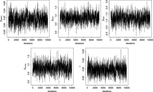
Figure 3: Trace plots of $\bolds{\beta}$ and $\gamma$ of the dynamic model with covariates.

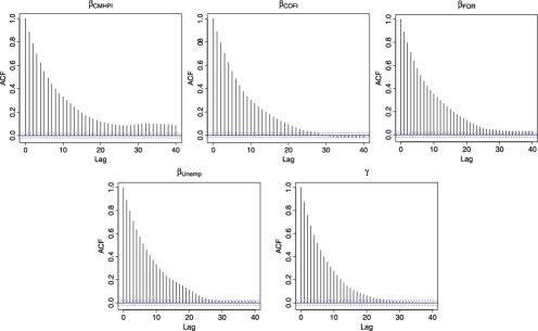
Figure 4: Autocorrelation plots of $\bolds{\beta}$ and $\gamma$ of the dynamic model with covariates.

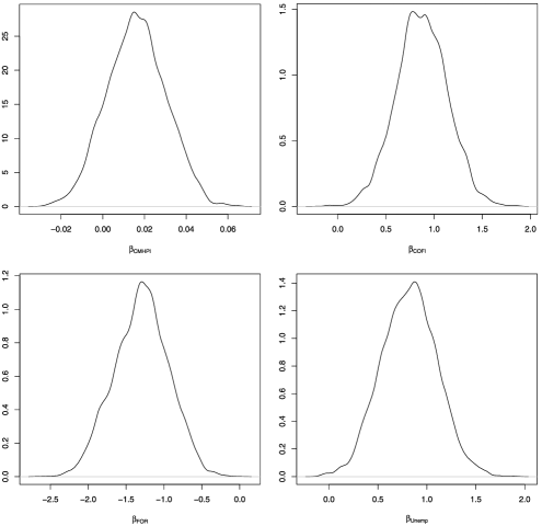
Figure 5: Posterior density plots of $\bolds{\beta}$ of the dynamic model with covariates.

Figure 6: Posterior density plot of $\gamma$ of the dynamic model with covariates.

The posterior density plots of $\bolds{\beta}$ are shown in Figure 5 and of $\gamma$ in Figure 6, which exhibits similar behavior to that of the posterior discounting term obtained for the dynamic model as in Figure 2.

As can be observed from Table 1, the $\beta$ coefficients all have fairly significant effects on the default rate. An advantage of the Bayesian approach is its ability to quantify posterior inference probabilistically. For instance, one can calculate the probability that $\beta_{\mathrm{CMHPI}}$ is greater than 0, that is, $p(\beta_{\mathrm{CMHPI}}>0|N^{(t)})$. Given the cohort at hand, $P(\beta_{\mathrm{CMHPI}}>0|N^{(t)})$ was obtained to be approximately 0.87, which shows strong evidence in favor of a positive effect. In summary, the regional conventional mortgage home price index (CMHPI), federal cost of funds index (COFI) and the regional unemployment rate (Unemp) have positive effects on default counts. For instance, as unemployment goes up, the model suggests that the number of people defaulting tends to increase for the cohort under study. On the other hand, the homeowner financial obligations ratio (FOR) seems to decrease the expected number of defaults as it goes up, namely, as the burden of repayment becomes relatively easier, then homeowners are less likely to default.

One of the issues that had been under investigation so far was the dynamic nature of the default rate. As shown in Figure 7, the fit of the dynamic model with covariates is reasonably good, justifying the dynamic behavior of the default rate. Similar conclusions can be drawn for the dynamic model without the covariates whose fit is shown in the right panel of Figure 2. In showing the dynamic nature of the default rate, we obtained the joint distribution of the baseline default rates, that is, $p(\theta_{1},\ldots,\theta_{t}|N^{(t)})$ as in (31). A boxplot of $\theta_{t}$s is shown in Figure 8, which once again provides strong evidence in favor of a dynamic default rate.

To investigate the existence of dynamic covariates, we estimated the model from Section 3.1. We once again assumed flat but proper priors as $\gamma\sim U(0,1)$ and $\tau_{i}\sim G(0.001,0.001)\ \forall i$. We note here that even though the use of the flat Gamma prior for $\tau_{i}$ is common in the literature, it has been known to have high concentration at very small values and very low probability everywhere else. However, our results were not influenced by the choice of the prior. The MCMC estimation was less straightforward as opposed to the model with static covariates. We ran the chain for 30,000 iterations as the burn-in period and we collected 50,000 observations with a thinning interval of 10. The mixing was slower since the full conditionals for each time dependent regression coefficient require a Metropolis–Hasting step. However, we did not encounter any convergence issues. In fact, having dynamic regression coefficients improved both the fit and the forecasting of the model as we discuss in the sequel.

Table 1: Posterior statistics for $\bolds{\beta}$ and $\gamma$ of the dynamic model with covariates

Statistics	$\bolds{\beta_{\mathrm{CMHPI}}}$	$\bolds{\beta_{\mathrm{COFI}}}$	$\bolds{\beta_{\mathrm{FOR}}}$	$\bolds{\beta_{\mathrm{Unemp}}}$	$\bolds{\gamma}$
25th	0.0063	0.7003	$-1.5430$	0.6252	0.2281
Mean	0.0160	0.8717	$-1.3002$	0.8191	0.2466
75th	0.0256	1.0510	$-1.0550$	1.0117	0.2643
St. Dev	0.0141	0.2663	$-$0.3606	0.2826	0.0270

Figure 7: Retrospective fit of the dynamic model with static covariate coefficients to data.

Figure 8: Boxplots for smoothed $\theta_{t}$s from $p(\theta_{1},\ldots,\theta_{t}|N^{(t)})$.

Table 2: $\operatorname{log}\{p(N^{(t)})\}$ and $\operatorname{log}(\mathrm{CPO})$ under each model

	DM1	DM2	DM3	DM4	DM5	BPM
$\operatorname{log}\{p(N^{(t)})\}$	$-579.99$	$-577.61$	$-577.67$	$-566.01$	$-541.74$	$-1416.28$
$\operatorname{log}(\mathrm{CPO})$	$-580.07$	$-578.69$	$-580.70$	$-572.28$	$-560.63$	$-1372.62$

Figure 9: Boxplots for the seasonal effects from DM4.

5.4 Model comparison

In order to compare the in-sample fit of the proposed models, we computed the log-marginal likelihoods as in (35) and the conditional predictive ordinates in the log-scale as in (36). In addition, we investigated presence of potential polynomial trends by adding a second order polynomial to our dynamic model with covariates and investigated the existence of seasonality by including 11 dummy variables for each month with month 12 being the reference period (as motivated by Figure 1). The results are shown in Table 2 where DM1 stands for the dynamic model, DM2 for the dynamic model with covariates, DM3 for the dynamic model with covariates and a second order polynomial trend, DM4 for the dynamic model with seasonality, DM5 for the dynamic model with dynamic covariate effects and BPM for Bayesian Poisson regression model. The dynamic model with dynamic covariate effects (DM5) has the highest log-marginal likelihood value and the highest CPO with a Bayes factor of $>$ 100 against its closest competitor ($\mathrm{BF}=\frac{p(N^{(t)}|\operatorname{DM4})}{p(N^{(t)}|\operatorname{DM2})}$), which, according to Kass and Raftery (1995), shows decisive support in favor of DM5. The results further support the lack of fit of the static model and show decisive evidence in favor of the dynamic models with Bayes factors of $>$ 100 against the Poisson regression model. Furthermore, adding a second order polynomial trend did not improve the model fit (the log-likelihoods of DM2 vs. DM3 are identical). However, adding the covariate information did improve the model fit (DM1 vs. DM2, DM3, DM4 and DM5). Even though the polynomial trend did not improve the model fit for this particular data set, capturing the monthly periodic effects did, as evidenced by the fit performance of model DM4 and the boxplot of its seasonal effects of Figure 9.

In addition to understanding the default behavior of a given cohort, it is also of interest to assess the model’s ability to predict future defaults for the cohort. In doing so, we considered two forecasting horizons: one during the earlier stages of the cohort (between the 35th and 44th months) and the second during the later stages (between the 135th and 144th months). For both forecast horizons, we sequentially predicted the next month without using the information of the future. For instance, we used the the first 34 months of data (both mortgage counts and covariates when needed) as a training data set to predict the 35th month and we sequentially predicted all 10 future months for both forecast horizons.

To provide one-month-ahead forecasting comparisons, we mainly considered two measures: the mean absolute percentage error (MAPE) and the root mean squared error (RMSE) calculated as

$$\operatorname{MAPE}=\frac{1}{H}\sum_{t=1}^{H}\frac{|N_{t}-E(N_{t}|N^{(t-1)})|}{N_{t}},$$ (38)

where $N_{t}$ is the actual default count observed during the month $t$ and $E(N_{t}|N^{(t-1)})$ is its one-month-ahead prediction. Similarly,

$$\operatorname{RMSE}=\sqrt{\frac{1}{H}\sum_{i=1}^{H}\bigl{\{}N_{t}-E\bigl{(}N_{t}|N^{(t-1)}\bigr{)}\bigr{\}}^{2}},$$ (39)

where $H$ represents the forecast horizon (in our example, $H=10$ for both forecast intervals cases). We also considered other measures of forecast performance such as the mean 95% coverage probability and the mean width of forecasts as in

$$\operatorname{MCov} = \frac{1}{H}\sum_{t=1}^{H}I\bigl{\{}\bigl{(}N^{2.5}_{t}|N^{(t)}\bigr{)}<N_{t}<\bigl{(}N^{97.5}_{t}|N^{(t)}\bigr{)}\bigr{\}}\quad\mbox{and}$$

$$\operatorname{MWid} = \frac{1}{H}\sum_{t=1}^{H}\bigl{(}N^{97.5}_{t}|N^{(t)}\bigr{)}-\bigl{(}N^{2.5}_{t}|N^{(t)}\bigr{)},$$

where $I(\cdot)$ is the indicator function, $(N^{97.5}_{t}|N^{(t)})$ and $(N^{2.5}_{t}|N^{(t)})$ are 97.5th and 2.5th quantiles of the forecasts for time $t$.

In addition to the dynamic models and the Poisson regression model, we considered using a simple time series model such as the exponentially weighted moving average (EWMA). To determine the smoothing constant for EWMA, we minimized the mean absolute percentage deviations, sequentially estimated it each time to predict the next month so that the models were comparable.

Table 3: Forecasting performance comparison

	Months 35–44						Months 135–144
	DM1	DM2	DM4	DM5	BPM	EWMA	DM1	DM2	DM4	DM5	BPM	EWMA
MAPE	$13.6$	$17.09$	$13.4$	$17.8$	$22.1$	$21.2$	$36.9$	$57.5$	$58.2$	$51.5$	$103.8$	$65.0$
RMSE	$21.9$	$29.3$	$20.3$	$31.7$	$36.03$	$39.20$	$2.77$	$3.09$	$3.30$	$3.02$	$4.96$	$3.86$
MCov	$1.00$	$0.40$	$0.50$	$0.30$	$0.20$	NA	$1.00$	$0.10$	$0.20$	$0.20$	$0.20$	NA
MWid	$121$	$11.4$	$37.40$	$16.20$	$22.39$	NA	$13.4$	$2.15$	$1.70$	$2.36$	$4.29$	NA

The results are shown in Table 3 where DM1, DM2, DM4 and DM5 exhibit better forecasting performance than BPM and EWMA for both forecast horizons. An interesting finding is that DM1 (model with no covariates) provides better forecasts for one of these two particular forecast horizons even though the overall model fit of DM2, DM4 and DM5 were concluded to be superior in Table 2. In addition, the mean coverage probabilities are both equal to 1 for DM1 since its prediction intervals are significantly wider than those of DM2, DM4 and DM5. This might be due to the small values of $\gamma$ which imply high discounting, leading to high uncertainty in the predictions. However, when we control for covariates and seasonal factors such uncertainty is diminished as evidenced by the prediction intervals given in Table 3. The narrowest prediction intervals are provided by DM4 for the 35–44 horizon and by DM2 for the 135–144 horizon. Also, adding the seasonal components significantly improved the forecasting performance of the dynamic models during the 35–44 month period where there is visual evidence of seasonality as shown in Figure 1. Toward the end of the series during the 135–144 month horizon, the default counts become more stable with no obvious seasonal patterns. Thus, the dynamic model with no covariates perform better due to its random walk type structure.

6 Concluding remarks

In this paper we considered discrete time Bayesian state space models with Poisson measurements to model the aggregate mortgage default risk. As pointed out by Kiefer (2011), the Bayesian approach provides a coherent framework to combine data with prior information and enables us to make inferences using probabilistic reasoning. In addition, the proposed state space models with stochastic default rate can capture the effects of correlated defaults over time. In order to carry out the inference of model parameters, we used Markov chain Monte Carlo methods such as the Gibbs sampler, Metropolis–Hastings and forward filtering backward sampling algorithms. In modeling the aggregate mortgage default risk, we addressed whether the default rate was exhibiting static or dynamic behavior and investigated the effects of macroeconomic variables on default risk. Strong evidence in favor of dynamic default behavior at the aggregate level was found. Furthermore, we found significant effects of macroeconomic variables such as the regional conventional mortgage home price index, federal cost of funds index, the homeowner mortgage financial obligations ratio and the regional unemployment rate on the aggregate mortgage default risk.

To the best of our knowledge, this is the first study using Bayesian state space models considered in the mortgage default risk literature at the aggregate level. Previous work mainly focuses on the individual default behavior of borrowers, and the effects of mortgage loan, property, borrower and economic characteristics on default risk. The only study which considers modeling the mortgage default risk at the aggregate level is due to Taufer (2007), who treats the default rate as a stochastic process and points out the need for models that will assist financial institutions to quantify mortgage default risk as required by the Basel III framework. Kiefer (2010, 2011) introduces a Bayesian binomial model for the default estimation of loan portfolios and their estimation using expert information. Although neither work focuses on mortgage default specifically, both highlight the need for models that can capture correlated default behavior in a pool of loan portfolios that are similar to mortgage cohorts consisting of several individual borrowers. In addition, none of these studies consider the effects of macroeconomic covariates on the default rate. In fact, Taufer (2007) comments on the lack and also on the need of covariate effects in his model. Our proposed state space models can easily take into account such covariate effects in both static and dynamic manners that are crucial in volatile economic environments. Thus, the novelty of our proposed models can be summarized as the introduction of Bayesian state space models with Poisson measurements to the mortgage default risk literature at the aggregate level, their ability to incorporate correlated mortgage defaults and to capture the effects of covariates on the default rate. In addition, the development of the Bayesian Poisson state space models and their estimation using MCMC methods are also modest contributions to the Poisson time series literature.

We believe that there are potential areas of research in modeling the mortgage risk at the aggregate level that we would like to pursue in the future. For instance, if information regarding the size of a given were available, then one can consider correlated state space binomial processes with both static and dynamic covariate effects to model the default counts and compare them with those presented in this paper. Although we did not encounter any efficiency issues in the use of MCMC methods with our current data, another potential area is to consider the use of particle filtering methods to speed up the convergence in sequential updating and forecasting for larger data sets.

References

- Ambrose and Capone (1998) {barticle}[auto:STB—2013/05/03—14:24:43] \bauthor\bsnmAmbrose, \bfnmB. W.\binitsB. W. and \bauthor\bsnmCapone, \bfnmC. A.\binitsC. A. (\byear1998). \btitleModeling the conditional probability of foreclosure in the context of single-family mortgage default resolutions. \bjournalReal Estate Economics \bvolume26 \bpages391–429. \bptokimsref \endbibitem
- Chib and Greenberg (1995) {barticle}[auto:STB—2013/05/03—14:24:43] \bauthor\bsnmChib, \bfnmS.\binitsS. and \bauthor\bsnmGreenberg, \bfnmE.\binitsE. (\byear1995). \btitleUnderstanding the Metropolis–Hasting algorithm. \bjournalAmer. Statist. \bvolume49 \bpages327–335. \bptokimsref \endbibitem
- Cox (1972) {bincollection}[mr] \bauthor\bsnmCox, \bfnmD. R.\binitsD. R. (\byear1972). \btitleThe statistical analysis of dependencies in point processes. In \bbooktitleStochastic Point Processes: Statistical Analysis, Theory, and Applications (Conf., IBM Res. Center, Yorktown Heights, NY, 1971) (\beditor\binitsP. A. W.\bfnmP. A. W. \bsnmLewis, ed.) \bpages55–66. \bpublisherWiley, \baddressNew York. \bidmr=0375705 \bptokimsref \endbibitem
- Cox (1981) {barticle}[mr] \bauthor\bsnmCox, \bfnmD. R.\binitsD. R. (\byear1981). \btitleStatistical analysis of time series: Some recent developments. \bjournalScand. J. Stat. \bvolume8 \bpages93–115. \bidissn=0303-6898, mr=0623586 \bptnotecheck related\bptokimsref \endbibitem
- Frühwirth-Schnatter (1994) {barticle}[mr] \bauthor\bsnmFrühwirth-Schnatter, \bfnmSylvia\binitsS. (\byear1994). \btitleData augmentation and dynamic linear models. \bjournalJ. Time Series Anal. \bvolume15 \bpages183–202. \biddoi=10.1111/j.1467-9892.1994.tb00184.x, issn=0143-9782, mr=1263889 \bptnotecheck year\bptokimsref \endbibitem
- Gelfand (1996) {bincollection}[mr] \bauthor\bsnmGelfand, \bfnmAlan E.\binitsA. E. (\byear1996). \btitleModel determination using sampling-based methods. In \bbooktitleMarkov Chain Monte Carlo in Practice \bpages145–161. \bpublisherChapman & Hall, \blocationLondon. \bidmr=1397969 \bptokimsref \endbibitem
- Gelfand, Dey and Chang (1992) {bincollection}[mr] \bauthor\bsnmGelfand, \bfnmA. E.\binitsA. E., \bauthor\bsnmDey, \bfnmD. K.\binitsD. K. and \bauthor\bsnmChang, \bfnmH.\binitsH. (\byear1992). \btitleModel determination using predictive distributions with implementation via sampling-based methods. In \bbooktitleBayesian Statistics, 4 (Peñíscola, 1991) (\beditor\binitsJ. M.\bfnmJ. M \bsnmBernardo, \beditor\binitsJ. O.\bfnmJ. O. \bsnmBerger, \beditor\binitsA. P.\bfnmA. P. \bsnmDawid and \beditor\binitsA. F. M.\bfnmA. F. M. \bsnmSmith, eds.) \bpages147–167. \bpublisherOxford Univ. Press, \blocationNew York. \bidmr=1380275 \bptokimsref \endbibitem
- Gelman et al. (1995) {bbook}[mr] \bauthor\bsnmGelman, \bfnmAndrew\binitsA., \bauthor\bsnmCarlin, \bfnmJohn B.\binitsJ. B., \bauthor\bsnmStern, \bfnmHal S.\binitsH. S. and \bauthor\bsnmRubin, \bfnmDonald B.\binitsD. B. (\byear1995). \btitleBayesian Data Analysis. \bpublisherChapman & Hall, \blocationLondon. \bidmr=1385925 \bptnotecheck year\bptokimsref \endbibitem
- Gilberto and Houston (1989) {barticle}[auto:STB—2013/05/03—14:24:43] \bauthor\bsnmGilberto, \bfnmS. M.\binitsS. M. and \bauthor\bsnmHouston, \bfnmA. L.\binitsA. L. (\byear1989). \btitleRelocation opportunities and mortgage default. \bjournalAREUEA Journal \bvolume17 \bpages55–69. \bptokimsref \endbibitem
- Herzog (1988) {barticle}[auto:STB—2013/05/03—14:24:43] \bauthor\bsnmHerzog, \bfnmT. N.\binitsT. N. (\byear1988). \btitleAnalyzing recent experience on FHA investor loans. \bjournalTransactions of Society of Actuaries \bvolume40 \bpages405–421. \bptokimsref \endbibitem
- Kass and Raftery (1995) {barticle}[auto:STB—2013/05/03—14:24:43] \bauthor\bsnmKass, \bfnmR. E.\binitsR. E. and \bauthor\bsnmRaftery, \bfnmA. E.\binitsA. E. (\byear1995). \btitleBayes factors. \bjournalJ. Amer. Statist. Assoc. \bvolume90 \bpages773–795. \bptokimsref \endbibitem
- Kau et al. (1990) {barticle}[auto:STB—2013/05/03—14:24:43] \bauthor\bsnmKau, \bfnmJ. B.\binitsJ. B., \bauthor\bsnmKeenan, \bfnmD. C.\binitsD. C., \bauthor\bsnmMuller-III, \bfnmW. J.\binitsW. J. and \bauthor\bsnmEpperson, \bfnmJ. F.\binitsJ. F. (\byear1990). \btitlePricing commercial mortgages and their mortgage backed securities. \bjournalThe Journal of Real Estate Finance and Economics \bvolume3 \bpages333–356. \bptokimsref \endbibitem
- Kiefer (2010) {barticle}[mr] \bauthor\bsnmKiefer, \bfnmNicholas M.\binitsN. M. (\byear2010). \btitleDefault estimation and expert information. \bjournalJ. Bus. Econom. Statist. \bvolume28 \bpages320–328. \biddoi=10.1198/jbes.2009.07236, issn=0735-0015, mr=2681204 \bptokimsref \endbibitem
- Kiefer (2011) {barticle}[mr] \bauthor\bsnmKiefer, \bfnmNicholas M.\binitsN. M. (\byear2011). \btitleDefault estimation, correlated defaults, and expert information. \bjournalJ. Appl. Econometrics \bvolume26 \bpages173–192. \biddoi=10.1002/jae.1124, issn=0883-7252, mr=2767466 \bptokimsref \endbibitem
- Lambrecht, Perraudin and Satchell (1997) {barticle}[auto:STB—2013/05/03—14:24:43] \bauthor\bsnmLambrecht, \bfnmB.\binitsB., \bauthor\bsnmPerraudin, \bfnmW.\binitsW. and \bauthor\bsnmSatchell, \bfnmS.\binitsS. (\byear1997). \btitleTime to default in the UK mortgage market. \bjournalEconomic Modeling \bvolume14 \bpages485–499. \bptokimsref \endbibitem
- Lambrecht, Perraudin and Satchell (2003) {barticle}[auto:STB—2013/05/03—14:24:43] \bauthor\bsnmLambrecht, \bfnmB.\binitsB., \bauthor\bsnmPerraudin, \bfnmW.\binitsW. and \bauthor\bsnmSatchell, \bfnmS.\binitsS. (\byear2003). \btitleMortgage default and possession under recourse: A competing hazards approach. \bjournalJournal of Money, Credit and Banking \bvolume35 \bpages425–442. \bptokimsref \endbibitem
- Leece (2004) {bbook}[auto:STB—2013/05/03—14:24:43] \bauthor\bsnmLeece, \bfnmD.\binitsD. (\byear2004). \btitleEconomics of the Mortgage Market: Perspectives on Household Decision Making. \bpublisherBlackwell, \blocationOxford. \bptokimsref \endbibitem
- Morali and Soyer (2003) {barticle}[mr] \bauthor\bsnmMorali, \bfnmNilgun\binitsN. and \bauthor\bsnmSoyer, \bfnmRefik\binitsR. (\byear2003). \btitleOptimal stopping in software testing. \bjournalNaval Res. Logist. \bvolume50 \bpages88–104. \biddoi=10.1002/nav.10048, issn=0894-069X, mr=1950283 \bptokimsref \endbibitem
- Popova, Popova and George (2008) {barticle}[mr] \bauthor\bsnmPopova, \bfnmIvilina\binitsI., \bauthor\bsnmPopova, \bfnmElmira\binitsE. and \bauthor\bsnmGeorge, \bfnmEdward I.\binitsE. I. (\byear2008). \btitleBayesian forecasting of prepayment rates for individual pools of mortgages. \bjournalBayesian Anal. \bvolume3 \bpages393–426. \biddoi=10.1214/08-BA315, issn=1936-0975, mr=2407432 \bptokimsref \endbibitem
- Quercia and Stegman (1992) {barticle}[auto:STB—2013/05/03—14:24:43] \bauthor\bsnmQuercia, \bfnmR. G.\binitsR. G. and \bauthor\bsnmStegman, \bfnmM. A.\binitsM. A. (\byear1992). \btitleResidential mortgage default: A review of the literature. \bjournalJournal of Housing Research \bvolume3 \bpages341–379. \bptokimsref \endbibitem
- Santos, Gamerman and Franco (2012) {bmisc}[auto:STB—2013/05/03—14:24:43] \bauthor\bsnmSantos, \bfnmT. R. D.\binitsT. R. D., \bauthor\bsnmGamerman, \bfnmD.\binitsD. and \bauthor\bsnmFranco, \bfnmG. C.\binitsG. C. (\byear2012). \bhowpublishedA non-Gaussian family of state-space models with exact marginal likelihood. Technical report. \bptokimsref \endbibitem
- Smith and Gelfand (1992) {barticle}[mr] \bauthor\bsnmSmith, \bfnmA. F. M.\binitsA. F. M. and \bauthor\bsnmGelfand, \bfnmA. E.\binitsA. E. (\byear1992). \btitleBayesian statistics without tears: A sampling-resampling perspective. \bjournalAmer. Statist. \bvolume46 \bpages84–88. \biddoi=10.2307/2684170, issn=0003-1305, mr=1165566 \bptokimsref \endbibitem
- Smith and Miller (1986) {barticle}[mr] \bauthor\bsnmSmith, \bfnmR. L.\binitsR. L. and \bauthor\bsnmMiller, \bfnmJ. E.\binitsJ. E. (\byear1986). \btitleA non-Gaussian state space model and application to prediction of records. \bjournalJ. R. Stat. Soc. Ser. B Stat. Methodol. \bvolume48 \bpages79–88. \bidissn=0035-9246, mr=0848053 \bptokimsref \endbibitem
- Soyer and Xu (2010) {barticle}[mr] \bauthor\bsnmSoyer, \bfnmRefik\binitsR. and \bauthor\bsnmXu, \bfnmFeng\binitsF. (\byear2010). \btitleAssessment of mortgage default risk via Bayesian reliability models. \bjournalAppl. Stoch. Models Bus. Ind. \bvolume26 \bpages308–330. \biddoi=10.1002/asmb.849, issn=1524-1904, mr=2682671 \bptokimsref \endbibitem
- Taufer (2007) {barticle}[mr] \bauthor\bsnmTaufer, \bfnmEmanuele\binitsE. (\byear2007). \btitleModelling stylized features in default rates. \bjournalAppl. Stoch. Models Bus. Ind. \bvolume23 \bpages73–82. \biddoi=10.1002/asmb.638, issn=1524-1904, mr=2344606 \bptokimsref \endbibitem
- Uhlig (1997) {barticle}[mr] \bauthor\bsnmUhlig, \bfnmHarald\binitsH. (\byear1997). \btitleBayesian vector autoregressions with stochastic volatility. \bjournalEconometrica \bvolume65 \bpages59–73. \biddoi=10.2307/2171813, issn=0012-9682, mr=1433685 \bptokimsref \endbibitem