Spatio-temporal exceedance locations and confidence regions

Abstract

An exceedance region is the set of locations in a spatial domain where a process exceeds some threshold. Examples of exceedance regions include areas where ozone concentrations exceed safety standards, there is high risk for tornadoes or floods, or heavy-metal levels are dangerously high. Identifying these regions in a spatial or spatio-temporal setting is an important responsibility in environmental monitoring. Exceedance regions are often estimated by finding the areas where predictions from a statistical model exceed some threshold. Even when estimation error is quantifiable at individual locations, the overall estimation error of the estimated exceedance region is still unknown. A method is presented for constructing a confidence region containing the true exceedance region of a spatio-temporal process at a certain time. The underlying latent process and any measurement error are assumed to be Gaussian. Conventional techniques are used to model the spatio-temporal data, and then conditional simulation is combined with hypothesis testing to create the desired confidence region. A simulation study is used to validate the approach for several levels of spatial and temporal dependence. The methodology is used to identify regions of Oregon having high precipitation levels and also used in comparing climate models and assessing climate change using climate models from the North American Regional Climate Change Assessment Program.

and

T1Supported under NSF Grant ATM-0534173.

1 Introduction

Identifying regions of extreme or unusual response is often a vital concern when analyzing environmental data. Identification of these regions can have important health, societal, and political impacts since these areas may indicate unusual events, outbreak of disease, toxic conditions, regions of extreme risk, etc. [Patil (2010)]. These regions of interest are often described as exceedance regions or hotspots, and are defined as the set of locations where the response process of interest exceeds some specified threshold. On the basis that the broad definition of exceed is “to go beyond the bounds or limits of” something [Dictionary.com (2012)], an exceedance region may refer to the area where the responses are above a threshold or the area where the responses fall below a threshold (though the two settings should be carefully distinguished).

The uncertainty associated with estimating exceedance regions has previously received relatively little attention. Our goal in this paper will be to introduce an approach for identifying exceedance regions with a quantifiable amount of certainty, and then using this methodology to confidently identify exceedance regions in two different contexts. First, in Section 4, this methodology will be used to confidently identify the regions of Oregon having extreme precipitation levels in October of 1998 using data from the previous two years. Being able to predict seasonal climate can help to minimize “climate surprises,” reduce impacts on society and ecosystems, assess the chances of events like drought and wildfire, and make important economic decisions in fields such as agriculture, energy, insurance, and public health [NOAA (2011)]. In Section 5, we use the proposed methodology to explore the temperature data of climate models from the North American Regional Climate Change Assessment Program (NARCCAP). Discussion will include assessment of future climate change for several regions of North America based on these models and also highlight similarities and differences between the projections from various climate models.

The methodology proposed in this article allows one to construct a confidence region for the exceedance region of a spatio-temporal process at a certain time. The resulting confidence region will contain the entire exceedance region with known confidence. To our knowledge, no methods have previously been available for constructing confidence regions containing the entire exceedance region of a spatial/spatio-temporal process and having the desired coverage properties. The methodology combines optimal spatio-temporal prediction methods and a hypothesis-testing-like approach to construct the confidence regions. Due to the simultaneous nature of the inference, the size and shape of the confidence regions will be directly related to the domain of interest. French (2012) introduced an approach for identifying the level curves of a spatial process with known confidence. Our methodology generalizes that of French (2012) by handling exceedance regions for spatio-temporal processes and also accounting for additional uncertainty when estimating the mean structure of the spatio-temporal process. The exceedance region of a spatial or spatio-temporal process is often predicted as the region(s) where the predicted response exceeds the desired threshold. This approach results in a biased predicted exceedance region since spatial predictors tend to oversmooth the response surface [Zhang, Cressie and Craigmile (2008)]. Craigmile et al. (2005) accounted for the oversmoothing of traditional spatial predictors by using a loss function that assigned more weight to extreme values in prediction; the predicted exceedance regions resulting from this approach are often larger than those of traditional methods. Patil and Taillie (2004) used the upper level set (ULS) scan statistic, a modification of the popular spatial scan statistic [Kulldorff and Nagarwalla (1995); Kulldorff (1997)] to identify regions or clusters of cells with elevated responses when compared to neighboring cells. The spatial scan statistic is often used in the setting where a region is tessellated into cells and response data are available as counts. Patil and Taillie (2004) used maximum likelihood estimation to identify regions with elevated counts through exhaustive search of the parameter space. The ULS scan statistic reduced the computational complexity of their task by reducing the search space, which allowed Patil and Taillie to construct a type of confidence region for the upper level sets (hotspots) by finding all zones where the ULS statistic was not statistically significant. The Progressive Upper Level Set (PULSE) scan statistic was recently proposed by Patil, Joshi and Koli (2010) as a refinement of the ULS statistic for detecting geospatial hotspots. Neither of the previous two approaches incorporates the typical notion of spatial dependence used to model and predict spatial data as exposited by Cressie (1993), Schabenberger and Gotway (2005), and many others. Zhang, Cressie and Craigmile (2008) predicted the exceedance region by finding the region minimizing the posterior loss of an image-based loss function using simulated annealing. The predicted exceedance region found by the approach of Zhang, Cressie and Craigmile (2008) is statistically optimal, but is not a confidence set in the traditional statistical sense. Recently, Sun et al. (2012) developed a unified theoretical and computational framework for false discovery control in multiple testing when trying to identify locations where the mean response of a process exceeds some threshold.

Other subject areas with connections to exceedance regions include the estimation of spatial cumulative distribution functions (CDFs) and the analysis of fMRI experiments to identify activated voxels. The spatial CDF of a process over a domain is a random distribution function that provides a statistical summary of a random field over a given region [Lahiri (1999)]. Spatial CDFs were introduced by Majure et al. (1996) and Lahiri (1999), and Lahiri et al. (1999) used subsampling approaches to predict a spatial CDF and study the asymptotic properties of the associated predictors. Zhu, Lahiri and Cressie (2002) developed an approach to detect a change in the spatial CDF of a region over time using the difference between two empirical CDFs and then quantified any change using the weighted integrated squared distance between the empirical CDFs. While spatial CDFs provide a way of identifying the proportion of a region exceeding some threshold, they do not identify where these exceedances occur. In the medical imaging field, there has long been an interest in identifying the areas of an fMRI map depicting brain activity in response to some stimuli. Marchini and Presanis (2004) provide a helpful overview of the various approaches to detecting active voxels. The most common approach for identifying active voxels is to declare a voxel active if some associated test statistic is above a single common threshold. This threshold is determined in a way that allows for control of some error criterion, such as the standard familywise error rate (FWER) or False Discovery Rate [FDR, Benjamini and Hochberg (1995)]. Often, the approach to determining this threshold utilizes the theory of random fields [Adler (2010), Adler and Taylor (2007)] and the expected Euler characteristic [Taylor, Worsley and Gosselin (2007), Adler (2008)] to determine the probability that the maximum test statistic is greater than some threshold. This approach can naturally apply in a geostatistical context such as the present one, but assumptions regarding the stationarity of the test statistics can be overly strict and often produces conservative results [Marchini and Presanis (2004)].

1.1 Outline

The approach proposed in this paper fills a methodological gap in the literature by allowing researchers to construct confidence regions for exceedance regions using traditional geostatistical tools and notions of spatial dependence while having the confidence level properties typically desired. The underlying latent process and any measurement error are assumed to be Gaussian.

This paper will proceed in the following manner. In Section 2 we will describe the proposed methodology in detail. Section 3 presents the results of a simulation study used to validate our approach, as well as several case studies exploring the shape of the confidence region for various underlying mean structures. Sections 4 and 5 describe applications of this methodology in the climatological settings mentioned above. We conclude with a brief discussion in Section 6.

2 Methodology

2.1 Framework

Consider a spatio-temporal response process $Y(\cdot,\cdot)\equiv\{Y(\mathbf{s},t),(\mathbf{s},t)\in D\times T\subset\mathbb{R}^{2}\times\mathbb{R}\}$, which has spatial index $\mathbf{s}$ contained in a bounded two-dimensional region of interest $D$, and time index $t$ which is contained in a bounded set of possible times $T\subset\mathbb{R}$. We assume that $Y(\cdot,\cdot)$ is the sum of a hidden spatio-temporal process $Z(\cdot,\cdot)$ and a measurement error process $\varepsilon(\cdot,\cdot),$ so that

$$Y(\mathbf{s},t)=Z(\mathbf{s},t)+\varepsilon(\mathbf{s},t),\qquad(\mathbf{s},t)\in D\times T.$$

We will refer to $Y(\cdot,\cdot)$ as the observable process and $Z(\cdot,\cdot)$ as the hidden or latent process. The hidden process $Z(\mathbf{s},t)$ is composed of a mean structure $\mu(\mathbf{s},t)$ capturing large-scale response behavior and a mean-zero spatio-temporal process $W(\mathbf{s},t)$ capturing small-scale behavior, such that $Z(\mathbf{s},t)$ can be decomposed into

$$Z(\mathbf{s},t)=\mu(\mathbf{s},t)+W(\mathbf{s},t),\qquad(\mathbf{s},t)\in D\times T.$$

The mean structure $\mu(\mathbf{s},t)$ is assumed to follow the linear model $\mu(\mathbf{s},t)=\mathbf{x}(\mathbf{s},t)^{\mathsf{T}}\bolds{\beta},$ where $\mathbf{x}(\mathbf{s},t)$ is a $k\times 1$ vector of known space–time covariates for location $\mathbf{s}$ at time $t$, $\bolds{\beta}$ is a vector of space–time trend parameters, and $W(\mathbf{s},t)$ is assumed to be a Gaussian process having continuous sample paths [cf. Paciorek (2003), page 57; Abrahamsen (1997), Adler and Taylor (2007)]. The covariance between two responses for the hidden process is denoted by

$$\operatorname{cov}\bigl{\{}Z(\mathbf{s}_{1},t_{1}),Z(\mathbf{s}_{2},t_{2})\bigr{\}}=C(\mathbf{s}_{1},\mathbf{s}_{2},t_{1},t_{2}).$$

The error process $\varepsilon(\mathbf{s},t)$ is assumed to be a Gaussian white-noise process with mean 0 and variance $\sigma_{\varepsilon}^{2}$, and the covariance between two responses of the observable process is given by

$$\operatorname{cov}\bigl{\{}Y(\mathbf{s}_{1},t_{1}),Y(\mathbf{s}_{2},t_{2})\bigr{\}}=C(\mathbf{s}_{1},\mathbf{s}_{2},t_{1},t_{2})+\sigma_{\varepsilon}^{2}v_{\varepsilon}(\mathbf{s}_{1},\mathbf{s}_{2},t_{1},t_{2}),$$

where $v_{\varepsilon}$ is a known function of the spatial and temporal indices (often returning 1 when $\mathbf{s}_{1}=\mathbf{s}_{2}$ and $t_{1}=t_{2}$ and zero otherwise).

Suppose we have observed $n$ responses $\mathbf{y}=[Y(\mathbf{s}_{1},t_{1}),\ldots,Y(\mathbf{s}_{n},t_{n})]^{\mathsf{T}}$ of a partial realization of $Y(\cdot,\cdot)$. Our goal is to use the observed responses to construct a confidence region for the locations where the hidden process $Z(\cdot,\cdot)$ exceeds some threshold $u$ at some time $t_{p}$. We define the exceedance region above a threshold $u$ for the hidden process $Z$ as $E_{u^{+}}^{Z}=\{\mathbf{s}\in D\dvtx Z(\mathbf{s},t_{p})\geq u\}$, while the exceedance region below a threshold $u$ may be defined as $E_{u^{-}}^{Z}=\{\mathbf{s}\in D\dvtx Z(\mathbf{s},t_{p})\leq u\}$. Depending on the exceedance region of interest (above or below the threshold), we would like to find a region $S_{u^{+}}$ that contains $E_{u^{+}}^{Z}$ with probability $1-\alpha$, that is, $P(E_{u^{+}}^{Z}\subseteq S_{u^{+}})=1-\alpha$ or a region $S_{u^{-}}$ that contains $E_{u^{-}}^{Z}$ with probability $1-\alpha$, that is, $P(E_{u^{-}}^{Z}\subseteq S_{u^{-}})=1-\alpha$.

2.2 Methodology

For simplicity, we will only describe methodology for determining the confidence region $S_{u^{+}}$ (the methodology for determining $S_{u^{-}}$ being analagous). Our approach for constructing our confidence region $S_{u^{+}}$ will combine geostatistical techniques along with an approach similar to hypothesis testing. We will state a null and alternative hypothesis, determine a test statistic and critical value, then make our conclusion. However, an important difference is that these tests are related to random variables instead of parameters, violating the classical definition of a hypothesis test. In spite of this difference, we will use the traditional terminology of hypothesis testing since the same concepts apply. Additionally, the procedure will call for a large number of statistical tests so the critical value must be adjusted in order to control the confidence level of our confidence region. We note that though this methodology is presented in the context of spatio-temporal processes, the approach is equally applicable to purely spatial data (with no time varying component) simply by assuming we have only one time.

The confidence region $S_{u^{+}}$ can be constructed by testing for each $\mathbf{s}\in D$, $H_{0}\dvtx Z(\mathbf{s},t_{p})=u$ versus $H_{a}\dvtx Z(\mathbf{s},t_{p})<u$ on the basis of a test statistic $Z^{\prime}(\mathbf{s},t_{p})$. The region $S_{u^{+}}$ is made up of all locations $\mathbf{s}$ where we fail to conclude that $Z(\mathbf{s},t_{p})<u$. Naturally, the test statistic $Z^{\prime}(\mathbf{s},t_{p})$ is based on a predictor of $Z(\mathbf{s},t_{p})$, $\hat{Z}(\mathbf{s},t_{p})$, from the statistical model outlined in Section 2.1. When the trend parameter vector $\bolds{\beta}$ must be estimated, the unbiased linear predictor of $Z(\mathbf{s},t)$ minimizing the mean-squared prediction error is known as the universal kriging predictor. Suppose we wish to make a prediction of $Z(\cdot,\cdot)$ at location $\mathbf{s}_{0}$ and time $t_{0}$. Let $\mathbf{x}_{0}$ denote the $k\times 1$ vector of space–time covariates associated with $Z(\mathbf{s}_{0},t_{0})$, $\mathbf{X}_{\mathbf{y}}$ denote the $n\times k$ matrix of covariates for the observed data $\mathbf{y}=\{Y(\mathbf{s}_{1},t_{1}),\ldots,Y(\mathbf{s}_{n},t_{n})\}$, $\bolds{\Sigma}_{\mathbf{y}}$ denote the $n\times n$ covariance matrix for the observed data $\mathbf{y}$, and

$$\mathbf{c}_{0\mathbf{y}}=\bigl{[}C(\mathbf{s}_{0},\mathbf{s}_{1},t_{0},t_{1}),\ldots,C(\mathbf{s}_{0},\mathbf{s}_{n},t_{0},t_{n})\bigr{]}^{\mathsf{T}}$$

be the $n\times 1$ vector of covariances between the response to be predicted and the observed data responses. The optimal predictor for $Z(\mathbf{s}_{0},t_{0})$ is

$$\hat{Z}(\mathbf{s}_{0},t_{0}) = \bolds{\Sigma}_{\mathbf{y}}^{-1}\bigl{(}\mathbf{c}_{0\mathbf{y}}-\mathbf{X}_{\mathbf{y}}\bigl{(}\mathbf{X}_{\mathbf{y}}^{\mathsf{T}}\bolds{\Sigma}_{\mathbf{y}}^{-1}\mathbf{X}_{\mathbf{y}}\bigr{)}^{-1}\bigl{(}\mathbf{X}_{\mathbf{y}}^{\mathsf{T}}\bolds{\Sigma}_{\mathbf{y}}^{-1}\mathbf{c}_{0\mathbf{y}}-\mathbf{x}_{0}\bigr{)}\bigr{)}\mathbf{y}$$

$$= \mathbf{x}_{0}^{\mathsf{T}}\hat{\bolds{\beta}}_{\mathrm{gls}}+\mathbf{c}_{0\mathbf{y}}^{\mathsf{T}}\bolds{\Sigma}_{\mathbf{y}}^{-1}(\mathbf{y}-\mathbf{X}_{\mathbf{y}}\hat{\bolds{\beta}}_{\mathrm{gls}}),$$

where $\hat{\bolds{\beta}}_{\mathrm{gls}}=(\mathbf{X}_{\mathbf{y}}^{\mathsf{T}}\bolds{\Sigma}_{\mathbf{y}}^{-1}\mathbf{X}_{\mathbf{y}})^{-1}\mathbf{X}_{\mathbf{y}}^{\mathsf{T}}\bolds{\Sigma}_{\mathbf{y}}^{-1}\mathbf{y}$ is the generalized least squares estimator of $\bolds{\beta}$. The associated mean-squared prediction error (kriging variance) of this predictor is given by

$$\sigma_{k}^{2}(\mathbf{s}_{0},t_{0}) = \sigma_{0}^{2}-\mathbf{c}_{0\mathbf{y}}^{\mathsf{T}}\Sigma_{\mathbf{y}}^{-1}\mathbf{c}_{0\mathbf{y}}$$

$${}+\bigl{(}\mathbf{x}_{0}-\mathbf{c}_{0\mathbf{y}}^{\mathsf{T}}\bolds{\Sigma}_{\mathbf{y}}^{-1}\mathbf{X}_{\mathbf{y}}\bigr{)}\bigl{(}\mathbf{X}_{\mathbf{y}}^{\mathsf{T}}\bolds{\Sigma}_{\mathbf{y}}^{-1}\mathbf{X}_{\mathbf{y}}\bigr{)}^{-1}\bigl{(}\mathbf{x}_{0}-\mathbf{c}_{0\mathbf{y}}^{\mathsf{T}}\bolds{\Sigma}_{\mathbf{y}}^{-1}\mathbf{X}_{\mathbf{y}}\bigr{)}^{\mathsf{T}},$$

where $\sigma_{0}^{2}=\operatorname{Var}(Z(\mathbf{s}_{0}))$ [Schabenberger and Gotway (2005), page 242]. Using the assumptions of normality made regarding $Z(\cdot,\cdot)$ and $\varepsilon(\cdot,\cdot)$, and using the properties of $\hat{Z}(\cdot,\cdot)$ and $\sigma_{k}(\cdot,\cdot)$, the quantity

$$\frac{\hat{Z}(\mathbf{s}_{0},t_{0})-Z(\mathbf{s}_{0},t_{0})}{\sigma_{k}(\mathbf{s}_{0},t_{0})}$$ (3)

has a standard Gaussian distribution. Assuming the null hypothesis is true, (3) leads us to the natural test statistic

$$Z^{\prime}(\mathbf{s}_{0},t_{0})=\frac{\hat{Z}(\mathbf{s}_{0},t_{0})-u}{\sigma_{k}(\mathbf{s}_{0},t_{0})}$$

for location $\mathbf{s}_{0}$ and time $t_{0}$.

The confidence level of our confidence region is controlled by carefully using the duality that exists between confidence intervals and hypothesis testing. Our confidence region $S_{u^{+}}$ is composed of all locations $\mathbf{s}$ where we fail to reject the null hypothesis that $Z(\mathbf{s},t_{p})=u$ [or perhaps more clearly, where we fail to reject that $Z(\mathbf{s},t_{p})\geq u$]. Thus, our confidence region will fail to contain the true exceedance region any time a Type I error is made in our hypothesis tests. In order to maintain a confidence level of $1-\alpha$ for our confidence region $S_{u^{+}}$, we must ensure that the probability of making a Type I error for all tests simultaneously is $\alpha$. Let $C_{\alpha}$ be the critical value at which we will reject $H_{0}$ and conclude $H_{a}.$ By definition, we can only make a Type I error at the locations $\mathbf{s}$ that are part of the true exceedance region. Consequently, when seeking to control our error rate, we are only concerned with controlling our error rate in the context of the possible realizations of $E_{u^{+}}^{Z}$ conditional on the observed data. Thus, to control the Type I error rate of our hypothesis at level $\alpha$ and maintain the confidence level of our confidence region at $1-\alpha$, we should only conclude $H_{a}$ when $Z^{\prime}(\mathbf{s},t_{p})<C_{\alpha}$, where $C_{\alpha}$ is chosen so that

$$P\Bigl{(}\inf_{\mathbf{s}\in E_{u^{+}}^{Z}}\bigl{\{}Z^{\prime}(\mathbf{s},t_{p})\bigr{\}}<C_{\alpha}\big{|}\mathbf{y}\Bigr{)}=\alpha.$$ (4)

2.3 Estimating the critical value $C_{\alpha}$ and constructing $S_{u^{+}}$

To properly estimate the critical value $C_{\alpha}$, we must be able to adequately approximate the distribution of

$$\inf_{\mathbf{s}\in E_{u^{+}}^{Z}}\bigl{\{}Z^{\prime}(\mathbf{s},t_{p})|\mathbf{y}\bigr{\}}$$ (5)

within our domain $D$. Note that the randomness of (5) is driven by the uncertainty in $E_{u^{+}}^{Z}$, not the uncertainty in $\{Z^{\prime}(\mathbf{s},t_{p})\}$. Conditional on the observed data, $\{Z^{\prime}(\mathbf{s},t_{p})\}$ is completely determined. In contrast, we do not know the exceedance region $E_{u^{+}}^{Z}$ generated in the same realization as the observed data $\mathbf{y}$. Though we are interested in the realization of $E_{u^{+}}^{Z}$ generated along with the actual data, there are infinitely many possible exceedance regions compatible with the observed data. Thus, we need to consider the distribution of $\inf_{\mathbf{s}\in E_{u^{+}}^{Z}}\{Z^{\prime}(\mathbf{s},t_{p})\}$ for all possible exceedance region realizations compatible with the observed data.

In practice, to estimate $C_{\alpha}$ in (4), we must assume that the behavior of the hidden process $Z(\cdot,t_{p})$ over the continuous domain $D$ can be adequately approximated by considering its behavior over an appropriately sized finite regular grid [cf. Zhang, Cressie and Craigmile (2008)]. We discretize the domain $D$ into $m$ pixels, letting $G=\{g_{1},\ldots,g_{m}\}$ be the set of pixels and $\mathbf{s}_{G}=\{\mathbf{s}_{1}^{*},\ldots,\mathbf{s}_{m}^{*}\}$ be the set of midpoints of these pixels. Let $\mathbf{z}_{G}=[Z(\mathbf{s}_{1}^{*},t_{p}),\ldots,Z(\mathbf{s}_{m}^{*},t_{p})]^{\mathsf{T}}$ denote the vector of hidden responses on the grid of locations $\mathbf{s}_{G}$. To approximate possible exceedance region realizations conditional on the observed data, we can simulate realizations of $\mathbf{z}_{G}|\mathbf{y}$ and determine the (discretized) exceedance regions for each realization.

The joint distribution of $\mathbf{z}_{G}$ and $\mathbf{y}$ is multivariate normal, making it straightforward to determine that the conditional distribution $\mathbf{z}_{G}|\mathbf{y}$ is also multivariate normal with closed form expressions for the associated mean and covariance matrix [Wasserman (2004), Theorem 2.44]. It is easy to simulate directly from a multivariate normal distribution using a decomposition of its covariance matrix [Givens and Hoeting (2005), page 146], but this does not take into account the fact that our mean function is being estimated. Instead, we will generate realizations of $\mathbf{z}_{G}|\mathbf{y}$ by conditioning our simulation using kriging. In essence, this approach produces realizations of the conditional distribution by perturbing the kriging estimates by possible realizations of the associated kriging error, as described below.

Suppose that

$$\left[\matrix{\mathbf{y}_{c}\vspace*{2pt}\cr\mathbf{z}_{c}}\right]\sim N\biggl{(}[\mathbf{0}],\left[\matrix{\bolds{\Sigma}_{\mathbf{y}}&\bolds{\Sigma}_{G\mathbf{y}}^{\mathsf{T}}\vspace*{2pt}\cr\bolds{\Sigma}_{G\mathbf{y}}&\bolds{\Sigma}_{G}}\right]\biggr{)},$$ (6)

recalling that $\bolds{\Sigma}_{\mathbf{y}}$ is the $n\times n$ covariance matrix of the observed data, and letting $\bolds{\Sigma}_{G}$ denote the $m\times m$ covariance matrix of $\mathbf{z}_{G}$ and $\bolds{\Sigma}_{G\mathbf{y}}$ denote the $m\times n$ cross-covariance matrix between $\mathbf{y}$ and $\mathbf{z}_{G}$. The joint distribution of $\mathbf{y}_{c}$ and $\mathbf{z}_{c}$ has the same covariance as the joint distribution of $\mathbf{y}$ and $\mathbf{z}_{G}$. To obtain $B$ realizations of $\mathbf{z}_{G}|\mathbf{y}$, we first use an extension of (2.2) allowing for simultaneous predictions at multiple locations [Schabenberger and Gotway (2005), pages 242–243] to find the $n\times m$ weight matrix $\bolds{\Lambda}$ such that $\hat{\mathbf{z}}_{G}=[\hat{Z}(\mathbf{s}_{1}^{*},t_{p}),\ldots,\hat{Z}(\mathbf{s}_{m},t_{p})]^{\mathsf{T}}=\bolds{\Lambda}^{\mathsf{T}}\mathbf{y}$. Next, we simulate $B$ realizations from the distribution in (6). Denote the first $n$ elements of the $i$th realization by $\mathbf{y}_{c}^{(i)}$ and the next $m$ elements by $\mathbf{z}_{c}^{(i)}$. The $i$th simulated realization of $\mathbf{z}_{G}|\mathbf{y}$ is then obtained using the expression

$$\tilde{\mathbf{z}}^{(i)}=\hat{\mathbf{z}}_{G}+\bigl{(}\mathbf{z}_{c}^{(i)}-\bolds{\Lambda}^{\mathsf{T}}\mathbf{y}_{c}^{(i)}\bigr{)},$$ (7)

with $[\tilde{Z}^{(i)}(\mathbf{s}_{1}^{*},t_{p}),\ldots,\tilde{Z}^{(i)}(\mathbf{s}_{m}^{*},t_{p})]^{\mathsf{T}}$ denoting the individual responses of this realization. The first part of expression (7) is the kriging predictor and the second part is a realization of possible kriging error. Additional information about this simulation process can be found in Chilès and Delfiner [(1999), pages 465–468].

To estimate $C_{\alpha}$, we begin by generating $B$ realizations $\{\tilde{\mathbf{z}}^{(1)},\ldots,\tilde{\mathbf{z}}^{(B)}\}$ of the conditional process $\mathbf{z}_{G}|\mathbf{y}$. For realization $i$, we identify $E_{u^{+}}^{\tilde{Z}^{(i)}}=\{\cup g_{j}\dvtx\break\tilde{Z}^{(i)}(\mathbf{s}_{j}^{*},t_{p})\geq u\}$, the union of the pixels where the simulated discretized conditional process exceeds the threshold $u$. For each realization of $E_{u^{+}}^{\tilde{Z}^{(i)}}$, we next consider the minimum of the test statistic $Z^{\prime}(\cdot,t_{p})$ at the gridded locations in the realized exceedance region under the assumption that the null hypothesis is true. Specifically, for each realization of $E_{u^{+}}^{\tilde{Z}^{(i)}}$ we find

$$\min_{\mathbf{s}\in\{\mathbf{s}_{G}\in E_{u^{+}}^{\tilde{Z}^{(i)}}\}}\bigl{\{}Z^{\prime}(\mathbf{s},t_{p})\bigr{\}}=\min_{\mathbf{s}\in\{\mathbf{s}_{G}\in E_{u^{+}}^{\tilde{Z}^{(i)}}\}}\biggl{\{}\frac{\hat{Z}(\mathbf{s},t_{p})-u}{\sigma_{k}(\mathbf{s},t_{p})}\biggr{\}}.$$

Last, $\hat{C}_{\alpha}$, our estimated value of $C_{\alpha}$, can be obtained by finding the $\alpha$ quantile of the set of minima from the previous step. The confidence region $S_{u^{+}}$ (or at least its discretized version) is then $S_{u^{+}}=\{\cup g_{i}\dvtx Z^{\prime}(\mathbf{s}_{i}^{*},t_{p})\geq\hat{C}_{\alpha}\}$.

2.4 Details of inference

We briefly summarize the inferences that can be made using the proposed methodology, as well as some details related to this inference.

2.4.1 Confidence region above

Using the methodology described above, one may construct a confidence region $S_{u^{+}}$ containing the realized exceedance region $E_{u^{+}}^{Z}$ with probability $1-\alpha$. Specifically, the probability that the confidence region $S_{u^{+}}$ produced by our method will contain the realized exceedance region $E_{u^{+}}^{Z}$ is $1-\alpha$, that is,

$$P\bigl{(}E_{u^{+}}^{Z}\subseteq S_{u^{+}}\bigr{)}=1-\alpha.$$ (8)

Note that the confidence properties of $S_{u^{+}}$ are in the frequentist paradigm. Thus, the probability in (8) may refer to the probability of $S_{u^{+}}$ containing the realized exceedance region before we collect the data or the long-term relative frequency of containing the realized exceedance region when applying this methodology to independent trials. A specific confidence region will either contain or not contain the true but unobserved realization of $E_{u^{+}}^{Z}$, but in repeated application of this methodology to new data sets, the long-term proportion of trials where the realized exceedance region will be entirely contained in the confidence region is $1-\alpha$.

2.4.2 Confidence region below

One may obtain a confidence region$S_{u^{-}}$ for the exceedance region below a threshold, $E_{u^{-}}^{Z}$, by considering the inverse of the problem described in Sections 2.2 and 2.3. By testing for all$\mathbf{s}\in D$, $H_{0}\dvtx Z(\mathbf{s},t_{p})\leq u$ versus $H_{a}\dvtx Z(\mathbf{s},t_{p})>u$ [and modifying the steps in Section 2.3 so that we approximate the critical value $C_{\alpha}$ such that$P(\sup_{\mathbf{s}\in E_{u^{-}}^{Z}}\{Z{}^{\prime}(\mathbf{s},t_{p})\}>C_{\alpha}|\mathbf{y})=\alpha$], we can construct a confidence region $S_{u^{-}}$ for $E_{u^{-}}^{Z}$ by letting $S_{u^{-}}=\{\mathbf{s}\in D\dvtx Z^{\prime}(\mathbf{s},t_{p})\leq C_{\alpha}\}$. This type of inference will be useful when one desires a confidence region for the entire area where a process may fall below some level, for example, identifying all locations where drought may occur. The confidence properties of $S_{u^{-}}$ are the same as those described for $S_{u^{+}}$ in Section 2.4.1.

2.4.3 Properties of the complement

The inference related to $S_{u^{+}}$ and $S_{u^{-}}$ is useful when one desires to find a region containing an entire exceedance region with high confidence. However, it is possible that a sizable portion of the confidence region is not part of the exceedance region and that the confidence region is much larger than the true exceedance region. Instead, we may be interested in the region of our domain $D$ where we can be confident that a response will exceed the threshold in question. This type of confidence region is easily obtained as a byproduct of the construction of $S_{u^{+}}$ and $S_{u^{-}}$.

Suppose we wish to find a confidence set contained entirely in $E_{u^{+}}^{Z}$, that is, every point in this confidence set has a response exceeding the threshold $u$. When constructing the confidence region $S_{u^{-}}$ for the locations having a response below the threshold $u$, $S_{u^{-}}$ has the property that $P(E_{u^{-}}^{Z}\subseteq S_{u^{-}})=1-\alpha$. Letting $S_{u^{-}}^{c}$ denote the complement of $S_{u^{-}}$, this implies that $P(\exists\mathbf{s}\in S_{u^{-}}^{c}\dvtx Z(\mathbf{s},t_{p})\leq u)=\alpha$, or, more naturally, $P(\forall\mathbf{s}\in S_{u^{-}}^{c}\dvtx Z(\mathbf{s},t_{p})>u)=1-\alpha$, which implies that

$$P\bigl{(}S_{u^{-}}^{c}\subseteq E_{u^{+}}^{Z}\bigr{)}=1-\alpha.$$

In other words, we can be confident that every point in $S_{u^{-}}^{c}$ simultaneously has a response exceeding the threshold $u$. Similar to the properties of the rejection region $S_{u^{-}}^{c}$, the rejection region $S_{u^{+}}^{c}$ has the property that every point in it will fall below the threshold $u$ with confidence.

By combining the information from $S_{u^{-}}^{c}$ with $S_{u^{+}}$, one may obtain a liberal and conservative view of where the realized exceedance region $E_{u^{+}}^{Z}$ may be located. Specifically, we can be confident (in a frequentist sense) that every point in $S_{u^{-}}^{c}$ is a member of the true exceedance set $E_{u^{+}}^{Z}$, but it is likely that $S_{u^{-}}^{c}$ is smaller than the true exceedance set. On the other hand, we can be confident that every location in $E_{u^{+}}^{Z}$ will be contained within $S_{u^{+}}$, but $S_{u^{+}}$ will likely be larger than $E_{u^{+}}^{Z}$. A similar interpretation applies to the regions $S_{u^{+}}^{c}$ and $S_{u^{-}}$ in relation to $E_{u^{-}}^{Z}$. Table 1 summarizes the methodology and inferences resulting from the proposed methodology.

Table 1: Summary of procedure and inferences for proposed methodology

	Exceedance above	Exceedance below
Region	$E_{u^{+}}^{Z}=\{\mathbf{s}\in D\dvtx Z(\mathbf{s},t_{p})\geq u\}$	$E_{u^{-}}^{Z}=\{\mathbf{s}\in D\dvtx Z(\mathbf{s},t_{p})\leq u\}$
$H_{0}$	$Z(\mathbf{s},t_{p})\geq u$	$Z(\mathbf{s},t_{p})\leq u$
$H_{a}$	$Z(\mathbf{s},t_{p})<u$	$Z(\mathbf{s},t_{p})>u$
Test stat.	$Z^{\prime}(\mathbf{s},t_{p})={\frac{Z(\mathbf{s},t_{p})-u}{\sigma_{k}(\mathbf{s},t_{p})}}$
Crit. value $C_{\alpha}$	$P(\inf_{\mathbf{s}\in E_{u^{+}}^{Z}}\{Z^{\prime}(\mathbf{s},t_{p})\}<C_{\alpha}|\mathbf{y})=\alpha$	$P(\sup_{\mathbf{s}\in E_{u^{-}}^{Z}}\{Z^{\prime}(\mathbf{s},t_{p})\}>C_{\alpha}|\mathbf{y})=\alpha$
Conf. region	$S_{u^{+}}=\{\mathbf{s}\in D\dvtx Z^{\prime}(\mathbf{s},t_{p})\geq C_{\alpha}\}$	$S_{u^{-}}=\{\mathbf{s}\in D\dvtx Z^{\prime}(\mathbf{s},t_{p})\leq C_{\alpha}\}$
Inference 1	$P(E_{u^{+}}^{Z}\subseteq S_{u^{+}})=1-\alpha$	$P(E_{u^{-}}^{Z}\subseteq S_{u^{-}})=1-\alpha$
Inference 2	$P(S_{u^{+}}^{c}\subseteq E_{u^{-}}^{Z})=1-\alpha$	$P(S_{u^{-}}^{c}\subseteq E_{u^{+}}^{Z})=1-\alpha$

2.4.4 Additional details

We note once again that the inference and properties of confidence regions discussed above are directly related to the domain in question. Since the procedure described in Section 2.3 depends on discretizing the domain of interest $D$, determining the realized exceedance regions $E_{u^{+}}^{\tilde{Z}^{(i)}}$ over that domain, estimating $C_{\alpha}$ over that domain, and evaluating the hypothesis tests over that domain, the confidence regions are directly linked to the domain chosen. This must be kept in mind when deciding on a domain of interest and considering the scope of inference.

We also note that the confidence properties above are dependent on knowing the true covariance properties of the random field under consideration. In practice, this is rarely the case. While it is typical to simply plug-in the estimated covariance parameters as if they were the truth [Schabenberger and Gotway (2005), page 254], this will likely result in confidence regions that have confidence levels differing from the desired levels. A Bayesian approach to this problem that naturally incorporates the uncertainty in the covariance parameters is currently under development.

3 Simulation studies

In this section we will use simulation experiments of the proposed methodology to compare empirical confidence levels to intended confidence levels for scenarios involving several combinations of mean structures and spatio-temporal dependence. In the experiments, the goal is to construct a confidence region $S_{u^{+}}$ containing the exceedance region $E_{u^{+}}^{Z}$ of the realization in question. The experiments are similar to ones performed by Zhang, Cressie and Craigmile (2008). Discussion will follow regarding how estimating the covariance parameters affects the empirical confidence levels and how the covariance parameters affect the shape and size of the confidence region for the true exceedance set. The analysis in Sections 3, 4, and 5 was performed using R version 2.15.1 [R Core Team (2012)].

3.1 Overall structure

In each of the subsequent experiments, the hidden process $Z(\cdot,\cdot)$ was assumed to follow the same general form

$$Z(\mathbf{s},t)=\mathbf{x}(\mathbf{s},t)^{\mathsf{T}}\bolds{\beta}+W(\mathbf{s},t).$$ (9)

The mean of $Z(\mathbf{s},t)$ was allowed to vary between four different patterns: trend, cone, cup, and waves. The domain $D$ of the experiment depended on the pattern under consideration. The mean structures of these patterns are shown in Figure 1, while the corresponding domain $D$ of the experiment, the covariate vector $\mathbf{x}(\mathbf{s},t)$, and coefficient vector $\bolds{\beta}$ of each pattern are provided in Table 2.

(a) Trend	(b) Cone	(c) Cup	(d) Waves

Figure 1: Mean structure of four different patterns.

Table 2: The domain $D$, covariates vector $\mathbf{x}(\mathbf{s},t)$, and coefficient vector $\bolds{\beta}$ used for the experiments of each pattern shown in Figure 1. The individual spatial coordinates of a spatial location $\mathbf{s}$ are denoted $\mathbf{s}_{x}$ and $\mathbf{s}_{y}$

Pattern	$\bolds{D}$	$\mathbf{x}\bolds{(}\mathbf{s},\bolds{t}\bolds{)}$	$\bolds{\beta}$
Trend	$[0,1]\times[0,1]$	$[1,\mathbf{s}_{x},\mathbf{s}_{x}]^{\mathsf{T}}$	$[1,3,3]^{\mathsf{T}}$
Cone	$[-0.5,0.5]\times[-0.5,0.5]$	$[1,\mathbf{s}_{x}^{2},\mathbf{s}_{y}^{2}]^{\mathsf{T}}$	$[1,-20,-20]^{\mathsf{T}}$
Cup	$[-0.5,0.5]\times[-0.5,0.5]$	$[1,\mathbf{s}_{x}^{2},\mathbf{s}_{y}^{2}]^{\mathsf{T}}$	$[1,20,20]^{\mathsf{T}}$
Waves	$[-\frac{3}{2}\pi,\frac{5}{2}\pi]\times[-2\pi,2\pi]$	$[1,\cos(\mathbf{s}_{x}),\sin(\mathbf{s}_{y})]^{\mathsf{T}}$	$[1,5,5]^{\mathsf{T}}$

The spatio-temporal process $W(\mathbf{s},t)$ was multivariate normal with mean 0 and isotropic covariance function

$$C(\mathbf{s}_{1}-\mathbf{s}_{2},t_{1}-t_{2})=\sigma_{W}^{2}\exp\bigl{(}\|\mathbf{s}_{1}-\mathbf{s}_{2}\|/\phi\bigr{)}\rho^{|t_{1}-t_{2}|},$$ (10)

where $\|\cdot\|$ is the Euclidean distance metric. This covariance function is obtained by multiplying an exponential covariance function $\exp(\|\mathbf{s}_{1}-\mathbf{s}_{2}\|/\phi)$ by $\rho^{|t_{1}-t_{2}|},$ the correlation function of an $\operatorname{AR}(1)$ temporal process. The strength of the spatial dependence is determined by $\phi$, and the strength of the temporal dependence is governed by $\rho$. In all experiments, the scale parameter $\sigma_{W}^{2}$ was fixed to be 1, while the spatial dependence parameter $\phi$ varied between the values $0.5$ (weak spatial dependence), $1.5$ (moderate spatial dependence), and 5 (very strong spatial dependence), and the temporal dependence parameter $\rho$ varied between the values $0.1$ (weak temporal dependence), $0.5$ (moderate temporal dependence), and 0.9 (strong temporal dependence). Experiments were performed assuming no measurement error ($\sigma_{\varepsilon}^{2}=0$) and when measurement error was present ($\sigma_{\varepsilon}^{2}=0.1$ or 0.5 depending on the mean structure).

In each experiment, the temporal window of interest $T=\{1,2,3,4\}$. It was assumed that responses with time index $t=1,2,3$ were observed data and that responses with time index $t=4$ corresponded to future responses. For each of the first three times, responses were observed at the same $100$ locations $\mathbf{s}_{1},\mathbf{s}_{2},\ldots,\mathbf{s}_{100}$. The sites of the 100 locations were irregularly spaced and were obtained by drawing independent observations from a $\operatorname{Uniform}(0,1)$ distribution and combining them to form a set of spatial coordinates. To apply the methodology described in Section 2 and obtain “future” data to test empirical confidence levels, the spatial domain for each experiment was discretized into a $50\times 50$ grid of pixels. For the trend pattern with domain $D=[0,1]\times[0,1]$, this resulted in the set of pixels $G=\{[x,x+0.02]\times[y,y+0.02]\dvtx x,y\in\{0,0.02,\ldots,0.98\}\}$, and the set of pixel center points $\mathbf{s}_{G}=\{(x,y)\dvtx x,y\in\{0.01,0.03,\ldots,0.99\}\}$. In the fourth year, future responses were “observed” at all locations $\mathbf{s}\in\mathbf{s}_{G}$ to provide the future test data. For each combination of covariance parameters $\phi$ and $\rho$, the hidden process $Z(\cdot,\cdot)$ was randomly generated at each of the 100 locations for the first three times, and then at the pixel center points for the fourth time. After generating the hidden process $Z(\cdot,\cdot)$, independent error values $\varepsilon_{1},\varepsilon_{2},\ldots,\varepsilon_{300}$ were generated according to a $N(0,\sigma_{\varepsilon}^{2})$ distribution and added to the 300 hidden process values observed for the first three times to obtain the observed response values $\mathbf{y}=\{Z(\mathbf{s}_{1},1)+\varepsilon_{1},\ldots,Z(\mathbf{s}_{100},1)+\varepsilon_{100},Z(\mathbf{s}_{1},2)+\varepsilon_{101},\ldots,Z(\mathbf{s}_{100},2)+\varepsilon_{200},Z(\mathbf{s}_{1},3)+\varepsilon_{201},\ldots,Z(\mathbf{s}_{100},3)+\varepsilon_{300}\}$. Note that the observed process recovers the hidden process when $\sigma_{\varepsilon}^{2}=0$.

The threshold level $u$ used to create the exceedance set $E_{u^{+}}^{Z}$ was the 90th percentile of the data generated on the $50\times 50$ grid for time $t=4$. Confidence regions $S_{u^{+}}$ were constructed at confidence levels of 0.90 and 0.95. For each experiment, the critical value $C_{\alpha}$ was estimated using 2000 realizations of $\mathbf{z}_{G}|\mathbf{y}$. Empirical confidence levels were calculated by generating 200 independent realizations of $Z(\cdot,\cdot)$ for each experimental setting, using the procedure of Section 2 to construct the confidence region $S_{u^{+}}$ for the exceedance region of the hidden process at time $t=4$, and then finding the proportion of realizations in which the confidence region $S_{u^{+}}$ contained the exceedance region $E_{u^{+}}^{Z}$.

3.2 Empirical confidence levels

For the trend pattern, experiments were run for all 9 combinations of the two dependence parameters $\phi$ and $\rho$. Experiments were run both without measurement error ($\sigma_{\varepsilon}^{2}=0$) and with measurement error ($\sigma^{2}=0.1$). In the initial experiments, it was assumed that the covariance parameters were all known. Subsequently, the same experiments were performed assuming that the covariance parameters were unknown. In the second set of experiments, the covariance parameters were estimated using restricted maximum likelihood (REML). The measurement error variance $\sigma_{\varepsilon}^{2}$ was estimated in each of these experiments, regardless of whether measurement error was actually present.

3.2.1 Results when covariance parameters known

The results of the simulation studies for the trend mean structure when the covariance parameters were assumed known are given below in Table 3. A comparative boxplot of the empirical confidence levels for these experiments grouped by desired confidence level is shown in Figure 2(a). The empirical confidence levels are all fairly close to the desired confidence level, and the empirical confidence levels behave in a manner consistent with sampling variability.

Table 3: Empirical coverage rate of confidence region procedure for trends simulation study. The standard error of the estimates are 2.12% for the 0.90 confidence level and 1.54% for the 0.95 confidence level

		Error variance	$\bolds{\sigma_{\varepsilon}^{2}}$	0			0.1
		Time dependence	$\bolds{\rho}$	0.1	0.5	0.9	0.1	0.5	0.9
Conf. level	0.90	Spat. depend. $\phi$	0.5	0.905	0.855	0.885	0.900	0.880	0.875
			1.5	0.910	0.915	0.905	0.870	0.890	0.860
			50.	0.885	0.910	0.890	0.870	0.915	0.920
	0.95	Spat. depend. $\phi$	0.5	0.960	0.915	0.960	0.940	0.940	0.930
			1.5	0.965	0.970	0.940	0.930	0.940	0.925
			50.	0.970	0.950	0.940	0.930	0.935	0.975

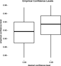
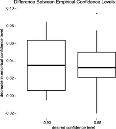
(a)	(b)

Figure 2: Boxplots of the empirical confidence levels for the confidence regions produced by the simulation study are shown by confidence level in (a). The change in empirical confidence level when estimated covariance parameters were used to construct the confidence regions is shown in (b).

3.2.2 Results when covariance parameters unknown

The covariance parameters of our data will not be known in practice, so we must use estimated values when making predictions. The empirical confidence level of the confidence regions of Section 2 are likely to be lower when estimated covariance parameter values are used instead of the true covariance parameter values. To get an idea of the magnitude of this drop, the simulation experiments for the trends mean structure of the previous section were repeated using estimated covariance parameters. Utilizing the same random number seed in each set of experiments, the observed data for the two sets of experiments was the same. The only difference in inference was that the covariance parameters were estimated via restricted maximum likelihood (REML) in the second set of experiments and then used in the construction of the confidence regions. Consequently, the results from the two experiments are paired. The differences between the empirical confidence levels for the two sets of experiments are displayed in the boxplot in Figure 2(b). The difference between the empirical confidence level for the two settings is typically between 0.01–0.07, though the values sometimes deviated from this range.

3.2.3 Computational cost

The proposed methodology has a computational cost essentially the same as that of the conditional simulation algorithm. As pointed out in the discussion of (7), the predicted responses and prediction weights are reused in the conditional simulation process. The only additional cost is the simulation of the unconditional random field in (6), and this cost can vary greatly depending on the algorithm selected. For the simulations described above, the prediction, conditional simulation, and construction of the confidence regions averaged just under 40 seconds on a MacBook Pro running OS X 10.7.4 with a 2.53 GHz Intel Core 2 Duo CPU and 4 GB of RAM. The same process averaged just over 3 seconds on a desktop PC running Fedora Core 16 with a 3.33 GHz Intel Core i7 CPU and 24 GB of RAM since many of the computations can run in parallel. The memory needed to construct the confidence regions depends directly on the number of observed and predicted data values and depends on the implementation of the proposed methodology. The conditional simulation process can be performed one at a time if necessary to minimize memory usage. However, for the simulation experiments performed in this section, the objects directly related to prediction, conditional simulation, and construction of the confidence regions required just over 38 MB of RAM.

3.3 Shapes

A question of interest is how the shape of the confidence region for the exceedance set is affected by factors such as the mean structure, spatio-temporal dependence, and error variance. We briefly studied the effects of these factors graphically using the cone, cup, and waves patterns discussed in Section 3.1. For these patterns, only the combinations of $(\phi,\rho)$ equal to (0.1, 0.1), (0.5, 0.5), (0.9, 0.9) were tested; we refer to these combinations of $(\phi,\rho)$ as weak, medium, and strong spatio-temporal dependence, respectively. The covariance parameters were assumed known in these additional experiments. In order to evaluate the the general shape of the confidence and exceedance regions for each mean structure, the 200 confidence regions and realized exceedance regions from each simulation experiment were used to construct a “median” exceedance region and confidence region. The “median” in each case was determined by noting the pixels where the realized exceedance region and/or confidence region appeared in at least half of the 200 realizations. Similarly, to evaluate how the strength of spatio-temporal dependence and measurement error affect the size of a confidence region, the number of pixels used to construct each confidence region for the 200 realizations of each experiment was also noted.

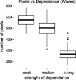
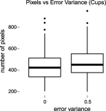
(a)	(b)	(c)

Figure 3: The median confidence region and exceedance set for the cone mean structure (medium dependence without measurement error) are shown in (a). Boxplots comparing the size of the confidence region (in number of pixels) versus the strength of dependence for the waves mean structure (without measurement error) for each of the 200 simulations are shown in (b). Boxplots comparing the size of the confidence region (in number of pixels) versus the measurement error variances for the cups mean structure (strong dependence) for each of the 200 simulations are shown in (c).

The shapes of the confidence and exceedance regions for the different mean structures conformed to intuitive expectations. Specifically, the confidence and exceedance regions of each shape patterned the mean structure. For example, the confidence and exceedance region for the cone mean structure were roughly circular since the exceedance region of the cone would simply be the upper portion of the cone. As an example of this, the median confidence region and exceedance set for the cone mean structure having medium spatial and temporal dependence without measurement error are shown in Figure 3(a). In order to assess the relationship between the strength of spatio-temporal dependence and the size of the resulting confidence region, as well as how measurement error affected these regions, we looked at the number of pixels in the confidence region from each of the 200 realizations of each experiment. Intuitively, stronger spatio-temporal dependence would lead to smaller predictive uncertainty, leading to a better estimate and smaller confidence region for the realized exceedance region. This pattern was consistently seen across all mean structures, and an example of this is shown in the boxplots in Figure 3(b) for the waves mean structure. Last, we would expect that the addition of measurement error to the observed responses would increase the size of the confidence regions due to greater uncertainty in predictions. This pattern was seen across all mean structures and levels of dependence, and an example of this for the cups mean structure is shown in Figure 3(c).

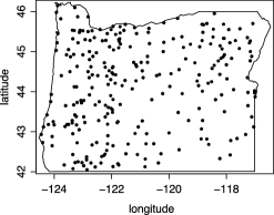
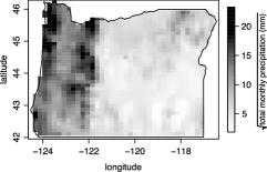
(a)	(b)

Figure 4: The observed data locations projected on a map of Oregon are shown in (a). An image plot of the average of the square root of the total monthly precipitation (mm) for the months of October 1996 and 1997 for the state of Oregon is shown in (b).

4 Case study 1: Precipitation in Oregon

We demonstrate application of this methodology using precipitation data from the state of Oregon. Our goal is to identify with 90% confidence the regions of Oregon where the total monthly precipitation exceeds 250 mm (approximately the 96th percentile of the observed data) in October of 1998 using the precipitation measurements available in October of 1996 and 1997. Analysis was performed using the raw data available at http://www.image.ucar.edu/Data/US.monthly.met/FullData.shtml#precip. The data used in this case study were created from the data archives of the National Climatic Data Center and have previously been used to generate high-resolution maps of precipitation and other meteorological variables [Daly et al. (2001), Johns et al. (2003)]. The raw data provides the longitude (degrees), latitude (degrees), and elevation (m) for 11,918 unique sites throughout the United States and, when available, includes the total monthly precipitation (mm) for each month between the years 1895–1997. There were 447 total observations provided for the state of Oregon between 1996 and 1997, with 191 observations in 1996 and 256 observations in 1997. The observed data locations are indicated by solid dots on a map of Oregon in Figure 4(a).

Exploratory analysis of the precipitation measurements revealed them to be positively skewed, so a square-root transformation of the measurements was taken to achieve approximate normality. An image plot of average precipitation for the transformed measurements is shown in Figure 4(b). Because the data were irregularly spaced, the bicubic spline interpolation algorithm of Akima (1996) was used to interpolate the average of the square root of the total monthly precipitation for the months of October 1996 and 1997 onto a regular grid before constructing the image plot.

The mean precipitation level of the responses $Z(\mathbf{s},t)$ was assumed to be the same for each year and follow the linear structure $\mu(\mathbf{s},t)=\mathbf{x}(\mathbf{s},t)^{\mathsf{T}}\bolds{\beta}$, with the covariates vector $\mathbf{x}(\mathbf{s},t)=[1,\mathrm{longitude},\mathrm{latitude},\mathrm{elevation}]^{\mathsf{T}}$. The covariance function of the hidden data was modeled as being stationary and fully separable with respect to space and time, while allowing for a spatio-temporal measurement error effect for the observed data that varied by year. Consequently, the covariance function of the observed data may be written as $C(\mathbf{s}_{1}-\mathbf{s}_{2},t_{1}-t_{2})=C_{S}(\mathbf{s}_{1}-\mathbf{s}_{2})C_{T}(t_{1}-t_{2})+C_{\varepsilon}(\mathbf{s}_{1}-\mathbf{s}_{2},t_{1}-t_{2})$, where $C_{S}(\cdot)$ is a purely spatial covariance function, $C_{T}(\cdot)$ is a purely temporal covariance function, and $C_{\varepsilon}(\cdot,\cdot)$ is the covariance function of the measurement errors. We assumed that the spatial covariance $C_{S}(\cdot)$ could be modeled using an isotropic, Matérn covariance model of the form $C_{S}(\mathbf{s}_{1},\mathbf{s}_{2})=\sigma^{2}2^{1-\nu}(h/\phi)^{\nu}\mathcal{K}_{\nu}(h/\phi)/\Gamma(\nu)$, where $h=\|\mathbf{s}_{1}-\mathbf{s}_{2}\|$ is the Euclidean distance between two data locations, $\phi$ is a parameter related to the strength of spatial dependence, $\sigma^{2}$ measures the variance of the hidden process $Z(\mathbf{s},t)$, $\nu$ controls the smoothness of the hidden process, and $\mathcal{K}_{\nu}(\cdot)$ is the modified Bessel function of the second kind of order $\nu$. The temporal covariance $C_{T}(t_{1},t_{2})$ was modeled using the correlation function of an $\operatorname{AR}(1)$ process so that $C_{T}(t_{1},t_{2})=\rho^{u}$, where $u=|t_{1}-t_{2}|$ is the time lag between $t_{1}$ and $t_{2}$ and $\rho$ measures the strength of spatial dependence. Last, the covariance function of the measurement errors can be written as

$$C_{\varepsilon}(\mathbf{s}_{1}-\mathbf{s}_{2},t_{1}-t_{2})=\bigl{[}\sigma_{96}^{2}\mathbf{1}_{(96)}(t_{1})+\sigma_{97}^{2}\mathbf{1}_{(97)}(t_{1})\bigr{]}\mathbf{1}_{(0,0)}(h,u),$$

where $\sigma_{96}^{2}$ and $\sigma_{97}^{2}$ are the variances of the measurement errors in years 1996 and 1997, respectively. Restricted maximum likelihood estimation was used to estimate the covariance parameters $\bolds{\theta}=[\sigma^{2},\phi,\nu,\rho,\sigma_{96}^{2},\sigma_{97}^{2}]^{\mathsf{T}}$, with the resulting estimates being

$$\hat{\bolds{\theta}}=[12.46,1.54,0.53,0.88,0.52,1.01]^{\mathsf{T}}.$$

Using the estimated covariance parameters to estimate the covariance matrix of the observed data, the generalized least squares estimates of the trend parameter vector $\bolds{\beta}$ is $\hat{\bolds{\beta}}_{\mathrm{gls}}=[-332.02,-2.17,1.73,0.0039]^{\mathsf{T}}$. Examining all of the available total monthly precipitation measurements for the month of October in the state of Oregon from 1895–1997, 250 mm of total rain corresponded to roughly the 96th percentile and was chosen as the exceedance threshold for which exceedance locations would be identified in October 1998. Accordingly, on the transformed scale our goal is to identify at a confidence level of 0.90 the exceedance region $E_{\sqrt{250}^{+}}^{Z}$ where the transformed total monthly precipitation measurements exceed $u=\sqrt{250\ \mathit{mm}}$.

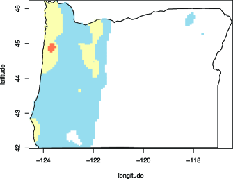
Figure 5: The 90 percent confidence regions $S_{\sqrt{250}^{+}}$ and $S_{\sqrt{250}^{-}}^{c}$ of Oregon where the square root of the total monthly precipitation (mm) in October of 1998 exceeds $\sqrt{250\ \mathit{mm}}$. The region $S_{\sqrt{250}^{+}}$ is colored blue, $S_{\sqrt{250}^{-}}^{c}$ is colored orange, while the region where the predicted values exceed $\sqrt{250\ \mathit{mm}}$ is colored yellow.

The next step in our analysis was creating a discrete grid in the region of interest $D$, where $D$ is the state of Oregon. For computational simplicity, a $100\times 100$ rectangular grid was superimposed over $D$, and the pixels with center points contained in $D$ were used as the discrete grid in subsequent analysis. Next, the procedure outlined in Section 2.3 was used to construct both $S_{\sqrt{250}^{+}}$ and $S_{\sqrt{250}^{-}}^{c}$ at a confidence level of 0.90 using 2000 realizations of (7); the resulting confidence regions are shown in Figure 5. The yellow coloring in Figure 5 indicates the regions where the predicted value (using universal kriging) is greater than the designated threshold, the blue coloring indicates the 90 percent confidence region $S_{\sqrt{250}^{+}}$, while orange coloring indicates the 90 percent confidence region $S_{\sqrt{250}^{-}}^{c}$. Naturally, the confidence region $S_{\sqrt{250}^{+}}$ contains the predicted exceedance region, while the predicted exceedance region contains $S_{\sqrt{250}^{-}}^{c}$. The area of Oregon predicted to have total monthly precipitation greater than 250 mm in October of 1998 is mainly limited to the western area of the state closer to the coast. The associated 90 percent confidence region $S_{\sqrt{250}^{+}}$ where 250 mm of rain could fall in October of 1998 is also found in the western portion of the state, though two small regions in the northeast corner of Oregon were also considered as possible candidates for this event. Only a small region (shown in orange) in the northwest part of the state could confidently be predicted to receive at least 250 mm of total monthly precipitation during this time period. On the other hand, the regions without any shading are the regions where we can be confident that total monthly precipitation will not exceed 250 mm, which comprises most of the eastern part of the state.

5 Case study 2: Regional climate projections

We continue to demonstrate the proposed methodology by using it to explore similarities and differences between projections of climate models from the North American Regional Climate Change Assessment Program [NARCCAP; Mearns et al. (2007), updated (2012)]. NARCCAP is an international, multi-disciplinary program exploring “separate and combined uncertainties in regional projections of future climate change resulting from the use of multiple atmosphere-ocean general circulation models (AOGCMs) to drive multiple regional climate models (RCMs)” as well as “to provide the climate impacts and adaptation community with high-resolution regional climate change scenarios that can be used for studies of the societal impacts of climate change and possible adaptation strategies” [Mearns et al. (2009); Mearns et al. (2012)]. Data produced by the program are available for numerous combinations of AOGCMS and RCMs, allowing researchers to investigate and study how various models interact, compare, and contrast with each other. Subsequent analysis will focus on combinations of two AOGCMs (CCSM and CGCM3) and four RCMs (CRCM, MM5I, RCM3, and WRFG) with a total of six models considered (CRCM/CCSM, CRCM/CGCM3, MM5I/CCSM, RCM3/CGCM3, WRFG/CCSM, and WRFG/CGCM3). We consider seasonal averages (Dec–Feb, Mar–May, Jun–Aug, Sep–Nov) of temperature (degrees Celsius) for years between 1971 and 2000 (note that the months are consecutive so that the December of the previous year is included in the average for the current year) on a 50 km grid covering Canada, the United States, and the northern part of Mexico. Projections from each model are also available for years between 2041 and 2070. Potential predictors to capture large-scale spatial trends include longitude, latitude, and elevation. The four main goals of this case study are to: [1.]

Compare and contrast the different AOGCM/RCM models to determine whether they portray the same type of behavior.

Explore the impact of season on climate predictions.

Study the effect of changing the threshold level on the associated exceedance region.

Assess where temperature increase is likely to occur based on these models. The size of the NARCCAP spatial grid and the wide variety of climatological conditions across the domain necessitated choices for how the data were analyzed. In order to capture the potential temperature increase between current and future model runs, future and current model runs were paired by differences of 70 years (e.g., the average winter temperature for 1971 was paired with the average winter temperature of 2041) and the difference between the future and current temperature values were taken. Depending on how the various RCMs were run, this left between 29 to 30 years of differences for each season. To simplify this part of the analysis, the data were separated into 9 year groupings (1971–1979/2041–2049, 1980–1988/2050–2058, and 1989–1997/2059–2067), and the average temperature difference for each season was calculated. Further, several smaller and climatologically consistent regions of the domain were analyzed individually to proceed with analysis. Examples of these smaller regions, Boreal, Central, Desert, East, MtWest, and South, are overlaid on a plot of North America in Figure 6. Using the averages from the three groupings of temperature, statistical inference for each region proceeded by predicting the average difference between seasonal temperature between the years 1998–2007 and 2068–2077, and constructing confidence regions for the exceedance regions of certain temperature thresholds. For the purposes of this paper, we will focus on results from the Boreal, South, and East regions during the winter and summer seasons.

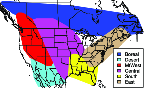
Figure 6: Individual NARCCAP regions analyzed.

Each climate model was analyzed in the following manner. The mean structure of the responses $Z(\mathbf{s},t)$ was assumed to be constant across nine-year groupings so that $\mu(\mathbf{s},t)=\mathbf{x}(\mathbf{s},t)^{\mathsf{T}}\bolds{\beta}$, where the covariates vector $\mathbf{x}(\mathbf{s},t)=[1,\mathrm{longitude},\mathrm{latitude},\mathrm{elevation}]^{\mathsf{T}}$. The covariance function of the observed data was modeled as being isotropic and fully separable with respect to space and time, using an exponential covariance structure for the spatial covariance and an $\operatorname{AR}(1)$ structure for the temporal covariance. Measurement error was assumed to have the same variance for all of the nine-year groupings. The covariance function of the observed data may be written as $C(\mathbf{s}_{1}-\mathbf{s}_{2},t_{1}-t_{2})=\sigma^{2}\exp(-h/\phi)\rho^{u}+\sigma_{\varepsilon}^{2}\mathbf{1}_{(0,0)}(h,u)$, where $h=\|\mathbf{s}_{1}-\mathbf{s}_{2}\|$ is the Euclidean distance between the two data locations and $u=|t_{1}-t_{2}|$ is the time lag between $t_{1}$ and $t_{2}$. Restricted maximum likelihood estimation was used to estimate the covariance parameters $\bolds{\theta}=[\sigma^{2},\phi,\rho,\sigma_{\varepsilon}^{2}]^{\mathsf{T}}$ assuming a multivariate Gaussian distribution for the observed responses.

The next step in our analysis was creating a discrete grid in the region of interest $D$, where $D$ is the individual region in question. Over each domain, a $100\times 100$ grid of regular pixels was overlaid, and then the center points of the pixels within the convex hull bounding the domain were retained for use as prediction locations. Following the procedure outlined in Section 2.3, confidence regions for the exceedance regions of the temperature change were constructed for levels $u=1$, 2, and 3^∘C using 10,000 realizations of the conditional random field in (7). For each region and exceedance level, both the region $S_{u^{+}}$ containing the true exceedance region $E_{u^{+}}^{Z}$ and the region $S_{u^{-}}^{c}$ for which all points in the region should be part of the exceedance region were obtained. The region $S_{u^{+}}$ is shown in blue and the region $S_{u^{-}}^{c}$ is shown in orange. Note that because of overlap, all orange locations are covering blue.

We begin by examining the effects of season on temperature predictions and the associated confidence regions for the Boreal region during the winter and summer seasons. The confidence regions associated with temperature change of at least $1^{\circ}$C in winter are shown in Figure 7(a), and for summer in (b).

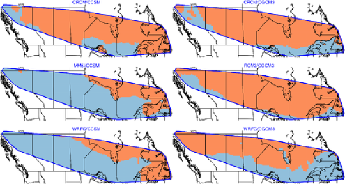
(a)

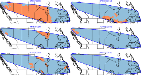
(b)

Figure 7: Confidence regions for locations in the Boreal region where temperature increase will be at least 1^∘C for various climate models. The results for winter are shown in (a) and for summer in (b). Blue shading indicates where the temperature increase may occur. Orange shading indicates where the temperature increase is likely to occur.

Comparing the graphs in Figure 7(a) and (b), the pattern of climate change is not necessarily consistent between winter and summer. Specifically, while the orange area (the area that we are confident will be part of the true exceedance region) for the winter data in Figure 7(a) is consistently in the northeastern area of the Boreal region, we do not see a similar pattern for the summer data in Figure 7(b). The areas that we can confidently identify as experiencing temperature increase in one season may not experience the same change in a different season. The confidence region $S_{1^{+}}$ (blue + orange) for the true exceedance set $E_{1^{+}}^{Z}$ during both winter and summer comprises the entire Boreal region. Consequently, any part of the Boreal region could experience a temperature increase of at least 1^∘C in both winter and summer. For the winter data, the orange region consistently makes up a large percentage of the northeastern Boreal region. Based on the agreement between these climate models, there appears to be high confidence that the northeastern part of the Boreal region will experience a temperature increase of at least 1^∘C when comparing the average winter temperature between the years 1989–1997 and 2059–2067. On the other hand, while several orange regions appear for the summer temperature data in Figure 7(b), there does not appear to be consistency between the various climate models. The CRCM/CCSM model results (upper left) in Figure 7(b) indicate that a majority of the region will experience temperature change of a least 1^∘C during the specified time period, while the WRFG/CGCM3 model does not indicate that any of the region will confidently experience this same change. While individual climate models may deem a certain region as being likely to experience a certain level of temperature increase, other climate models may paint a different picture.

We next consider temperature change in the South region, which comprises much of the southeastern part of the United States, and focus on how different RCM/AOGCM climate model combinations can make fairly different predictions. The results for temperature change of at least 3^∘C during winter and summer are shown in Figure 8(a) and (b), respectively.

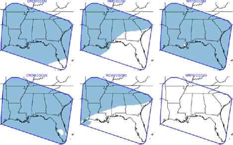
(a)

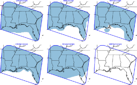
(b)

Figure 8: Confidence regions for locations in the South region where temperature increase will be at least 3^∘C for various climate models. The results for winter are shown in (a) and for summer in (b). Blue shading indicates where the temperature increase may occur. Areas without shading are regions where the temperature increase is unlikely to occur.

In the South region, the potential temperature increase portrayed by the climate models is fairly consistent from winter to summer. Additionally, the results for each of the climate models appear relatively similar with the exception of the WRFG/CGCM3 combination. Specifically, this combination predicts temperature increase in the South region as being smaller than each of the other climate models. This difference cannot be explained by the use of the CGCM3 AOGCM or WRFG RCM alone, since other model combinations having these model components do not behave in the same manner. This specific RCM/AOGCM combination interacts in a way that yields fairly different results than the other combinations considered. We note that the nonshaded regions are the regions confidently identified as not having a temperature increase of $3^{\circ}$C or more.

Last, we consider the effect of changing the threshold level on the resulting confidence region for the exceedance region by looking at results for the East region along the Eastern seaboard of the United States and Canada. Results for winter temperature increases of 1, 2, and 3^∘C are shown in Figure 9(a), (b), and (c), respectively. For all three thresholds, only the northeast part of the East region confidently has temperature increases exceeding the threshold in question (the areas shown in orange). However, as the temperature threshold increases, the size of the orange area decreases. This behavior is sensible since the more extreme a threshold is, the less likely it is that a response will exceed that threshold. Consequently, the orange areas where we are confident a response exceeds a threshold become smaller as the threshold increases. Based on the observation that the orange and blue shaded regions make up nearly the entire East region for all three thresholds, nearly any part of the East region of North America may experience an average temperature increase of at least 3^∘C when comparing the winter temperature between the years 1989–1997 and 2059–2067. On the other hand, since the orange area is mostly limited to the northeastern part of the East region for a threshold of 1^∘C, this is the only region the climate models can confidently identify as experiencing a temperature increase of at least 1^∘C. On the other hand, as the temperature threshold is increased to $3^{\circ}$C, some areas have no shading. These are the regions that can be confidently identified as not experiencing a temperature increase of $3^{\circ}$C or more. However, the nonshaded regions are not consistent between the various AOGCM/RCM combinations.

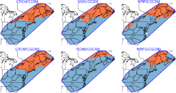
(a)

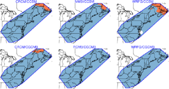
(b)

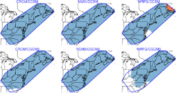
(c)

Figure 9: Confidence regions for locations in the East region where winter temperature increase will be at least 1^∘C, 2^∘C, and 3^∘C are shown in (a), (b), and (c), respectively. Blue shading indicates where the temperature increase may occur. Orange shading indicates where the temperature increase is likely to occur. Areas without shading are regions where the temperature increase is unlikely to occur.

We point out that the large blue regions in the preceding discussion may not be precise indicators of the size of the true exceedance region. The large size of the blue regions may simply be an indication of high uncertainty, since the size of the confidence regions $S_{u^{+}}$ will increase with elevated uncertainty.

6 Discussion

We have presented an approach for constructing confidence regions containing the entire exceedance region of a random field. Additionally, by considering the inverse problem, one may also obtain a region where all locations in the region will confidently be part of the exceedance region of the random field. This allows researchers to compare regions where it is possible for an extreme event to occur to the regions where it is likely that an extreme event will occur. The size of the confidence region naturally depends on factors such as the number of observed responses, the spatial and temporal dependence, and the magnitude of measurement error variance. Simulation experiments in Section 3.2 indicate that the procedure produces confidence regions having the appropriate coverage properties. Though all of these experiments used stationary latent processes for simplicity, stationarity is not required and simulation experiments for nonstationary processes have produced similar results. As further explored in Section 3.3, the shape of a confidence region naturally patterns itself after the underlying mean structure.

Using the proposed procedure, we were able to make inference about the regions of Oregon receiving 250 mm of precipitation in October of 1998. It also allowed us to compare climate models and explore future climate change for several combinations of RCMs and AOGCMs using models from NARCCAP. Though the statistical models used were basic, the results from these models supported the view that temperature increases of several degrees are possible for large parts of North America, and that certain areas seem likely to experience temperature change of several degrees. The analysis also revealed that there can be somewhat large discrepancies between climate models (the South region being a clear example).

It should be mentioned that the assumption that the spatio-temporal covariance functions of the statistical models were separable may be unnecessarily restrictive. Nonseparable and/or nonstationary spatio-temporal covariance models such as the ones proposed by Gneiting (2002) or Fuentes, Chen and Davis (2008) are possible alternatives. Additionally, the confidence regions were often quite large. This often was a consequence of the fact that most of the region in question was predicted to be greater than the exceedance threshold, but was sometimes a result of high predictive uncertainty in the areas. This suggests that similar tools with less stringent error criteria [e.g., Sun et al. (2012)] would be useful for climate model exploration. Related to this is the fact that more data brings more information and, consequently, may reduce the size of the confidence regions. Due to the size and complexity of the NARCCAP model output, specific regions of North America were analyzed in isolation. If the proposed procedure were extended to incorporate reduced rank modeling procedures such as fixed-rank kriging [Cressie and Johannesson (2008)] or fixed-rank filtering [Cressie, Shi and Kang (2010)], this limitation could be ameliorated, and this is the subject of ongoing research efforts. Additionally, it was pointed out in Section 2.4.4 that the confidence levels of the proposed methodology assumed that the covariance function of the random process was known, which is rarely the case. A Bayesian approach to this problem that naturally incorporates the uncertainty of the covariance function is under investigation.

References

- Abrahamsen (1997) {bmisc}[author] \bauthor\bsnmAbrahamsen, \bfnmPetter\binitsP. (\byear1997). \btitleA review of Gaussian random fields and correlation functions. Unpublished manuscript. \bptokimsref \endbibitem
- Adler (2008) {barticle}[mr] \bauthor\bsnmAdler, \bfnmRobert J.\binitsR. J. (\byear2008). \btitleSome new random field tools for spatial analysis. \bjournalStoch. Environ. Res. Risk Assess. \bvolume22 \bpages809–822. \biddoi=10.1007/s00477-008-0242-6, issn=1436-3240, mr=2430406 \bptokimsref \endbibitem
- Adler (2010) {bbook}[author] \bauthor\bsnmAdler, \bfnmR. J.\binitsR. J. (\byear2010). \btitleThe Geometry of Random Fields. \bpublisherSIAM, \blocationPhiladelphia. \bptokimsref \endbibitem
- Adler and Taylor (2007) {bbook}[mr] \bauthor\bsnmAdler, \bfnmRobert J.\binitsR. J. and \bauthor\bsnmTaylor, \bfnmJonathan E.\binitsJ. E. (\byear2007). \btitleRandom Fields and Geometry. \bpublisherSpringer, \blocationNew York. \bidmr=2319516 \bptokimsref \endbibitem
- Akima (1996) {barticle}[author] \bauthor\bsnmAkima, \bfnmH.\binitsH. (\byear1996). \btitleAlgorithm 761: Scattered-data surface fitting that has the accuracy of a cubic polynomial. \bjournalACM Trans. Math. Software \bvolume22 \bpages362–371. \bptokimsref \endbibitem
- Benjamini and Hochberg (1995) {barticle}[mr] \bauthor\bsnmBenjamini, \bfnmYoav\binitsY. and \bauthor\bsnmHochberg, \bfnmYosef\binitsY. (\byear1995). \btitleControlling the false discovery rate: A practical and powerful approach to multiple testing. \bjournalJ. R. Stat. Soc. Ser. B Stat. Methodol. \bvolume57 \bpages289–300. \bidissn=0035-9246, mr=1325392 \bptokimsref \endbibitem
- Chilès and Delfiner (1999) {bbook}[mr] \bauthor\bsnmChilès, \bfnmJean-Paul\binitsJ.-P. and \bauthor\bsnmDelfiner, \bfnmPierre\binitsP. (\byear1999). \btitleGeostatistics: Modeling Spatial Uncertainty. \bpublisherWiley, \blocationNew York. \biddoi=10.1002/9780470316993, mr=1679557 \bptokimsref \endbibitem
- Craigmile et al. (2005) {barticle}[mr] \bauthor\bsnmCraigmile, \bfnmPeter F.\binitsP. F., \bauthor\bsnmCressie, \bfnmNoel\binitsN., \bauthor\bsnmSantner, \bfnmThomas J.\binitsT. J. and \bauthor\bsnmRao, \bfnmYoulan\binitsY. (\byear2005). \btitleA loss function approach to identifying environmental exceedances. \bjournalExtremes \bvolume8 \bpages143–159. \biddoi=10.1007/s10687-006-7964-y, issn=1386-1999, mr=2275915 \bptokimsref \endbibitem
- Cressie (1993) {bbook}[mr] \bauthor\bsnmCressie, \bfnmNoel A. C.\binitsN. A. C. (\byear1993). \btitleStatistics for Spatial Data. \bpublisherWiley, \blocationNew York. \bidmr=1239641 \bptokimsref \endbibitem
- Cressie and Johannesson (2008) {barticle}[mr] \bauthor\bsnmCressie, \bfnmNoel\binitsN. and \bauthor\bsnmJohannesson, \bfnmGardar\binitsG. (\byear2008). \btitleFixed rank kriging for very large spatial data sets. \bjournalJ. R. Stat. Soc. Ser. B Stat. Methodol. \bvolume70 \bpages209–226. \biddoi=10.1111/j.1467-9868.2007.00633.x, issn=1369-7412, mr=2412639 \bptokimsref \endbibitem
- Cressie, Shi and Kang (2010) {barticle}[mr] \bauthor\bsnmCressie, \bfnmNoel\binitsN., \bauthor\bsnmShi, \bfnmTao\binitsT. and \bauthor\bsnmKang, \bfnmEmily L.\binitsE. L. (\byear2010). \btitleFixed rank filtering for spatio-temporal data. \bjournalJ. Comput. Graph. Statist. \bvolume19 \bpages724–745. \biddoi=10.1198/jcgs.2010.09051, issn=1061-8600, mr=2732500 \bptokimsref \endbibitem
- Daly et al. (2001) {barticle}[author] \bauthor\bsnmDaly, \bfnmC.\binitsC., \bauthor\bsnmTaylor, \bfnmG. H.\binitsG. H., \bauthor\bsnmGibson, \bfnmW. P.\binitsW. P., \bauthor\bsnmParzybok, \bfnmT. W.\binitsT. W., \bauthor\bsnmJohnson, \bfnmG. L.\binitsG. L. and \bauthor\bsnmPasteris, \bfnmP. A.\binitsP. A. (\byear2001). \btitleHigh-quality spatial climate data sets for the United States and beyond. \bjournalTransactions of the American Society of Agricultural Engineers \bvolume43 \bpages1957–1962. \bptokimsref \endbibitem
- Dictionary.com (2012) {bmisc}[author] \bauthor\bsnmDictionary. com (\byear2012). \bhowpublishedExceed. Dictionary.com unabridged. Accessed June 5, 2012. \bptokimsref \endbibitem
- French (2012) {bmisc}[author] \bauthor\bsnmFrench, \bfnmJ. P.\binitsJ. P. (\byear2012). \btitleConfidence regions for the level curves of spatial data. Available at http://math.ucdenver.edu/~jfrench. \bptokimsref \endbibitem
- Fuentes, Chen and Davis (2008) {barticle}[mr] \bauthor\bsnmFuentes, \bfnmMontserrat\binitsM., \bauthor\bsnmChen, \bfnmLi\binitsL. and \bauthor\bsnmDavis, \bfnmJerry M.\binitsJ. M. (\byear2008). \btitleA class of nonseparable and nonstationary spatial temporal covariance functions. \bjournalEnvironmetrics \bvolume19 \bpages487–507. \biddoi=10.1002/env.891, issn=1180-4009, mr=2523910 \bptokimsref \endbibitem
- Givens and Hoeting (2005) {bbook}[mr] \bauthor\bsnmGivens, \bfnmGeof H.\binitsG. H. and \bauthor\bsnmHoeting, \bfnmJennifer A.\binitsJ. A. (\byear2005). \btitleComputational Statistics. \bpublisherWiley, \blocationHoboken, NJ. \bidmr=2112774 \bptokimsref \endbibitem
- Gneiting (2002) {barticle}[mr] \bauthor\bsnmGneiting, \bfnmTilmann\binitsT. (\byear2002). \btitleNonseparable, stationary covariance functions for space–time data. \bjournalJ. Amer. Statist. Assoc. \bvolume97 \bpages590–600. \biddoi=10.1198/016214502760047113, issn=0162-1459, mr=1941475 \bptokimsref \endbibitem
- Johns et al. (2003) {barticle}[mr] \bauthor\bsnmJohns, \bfnmCraig J.\binitsC. J., \bauthor\bsnmNychka, \bfnmDouglas\binitsD., \bauthor\bsnmKittel, \bfnmTimothy G. F.\binitsT. G. F. and \bauthor\bsnmDaly, \bfnmChris\binitsC. (\byear2003). \btitleInfilling sparse records of spatial fields. \bjournalJ. Amer. Statist. Assoc. \bvolume98 \bpages796–806. \biddoi=10.1198/016214503000000729, issn=0162-1459, mr=2055488 \bptokimsref \endbibitem
- Kulldorff (1997) {barticle}[mr] \bauthor\bsnmKulldorff, \bfnmMartin\binitsM. (\byear1997). \btitleA spatial scan statistic. \bjournalComm. Statist. Theory Methods \bvolume26 \bpages1481–1496. \biddoi=10.1080/03610929708831995, issn=0361-0926, mr=1456844 \bptokimsref \endbibitem
- Kulldorff and Nagarwalla (1995) {barticle}[pbm] \bauthor\bsnmKulldorff, \bfnmM.\binitsM. and \bauthor\bsnmNagarwalla, \bfnmN.\binitsN. (\byear1995). \btitleSpatial disease clusters: Detection and inference. \bjournalStat. Med. \bvolume14 \bpages799–810. \bidissn=0277-6715, pmid=7644860 \bptokimsref \endbibitem
- Lahiri (1999) {barticle}[mr] \bauthor\bsnmLahiri, \bfnmS. N.\binitsS. N. (\byear1999). \btitleAsymptotic distribution of the empirical spatial cumulative distribution function predictor and prediction bands based on a subsampling method. \bjournalProbab. Theory Related Fields \bvolume114 \bpages55–84. \biddoi=10.1007/s004400050221, issn=0178-8051, mr=1697139 \bptokimsref \endbibitem
- Lahiri et al. (1999) {barticle}[mr] \bauthor\bsnmLahiri, \bfnmSoumendra N.\binitsS. N., \bauthor\bsnmKaiser, \bfnmMark S.\binitsM. S., \bauthor\bsnmCressie, \bfnmNoel\binitsN. and \bauthor\bsnmHsu, \bfnmNan-Jung\binitsN.-J. (\byear1999). \btitlePrediction of spatial cumulative distribution functions using subsampling. \bjournalJ. Amer. Statist. Assoc. \bvolume94 \bpages86–110. \biddoi=10.2307/2669680, issn=0162-1459, mr=1689216 \bptnotecheck related\bptokimsref \endbibitem
- Majure et al. (1996) {barticle}[author] \bauthor\bsnmMajure, \bfnmJ. J.\binitsJ. J., \bauthor\bsnmCook, \bfnmD.\binitsD., \bauthor\bsnmCressie, \bfnmN.\binitsN., \bauthor\bsnmKaiser, \bfnmM. S.\binitsM. S., \bauthor\bsnmLahiri, \bfnmS. N.\binitsS. N. and \bauthor\bsnmSymanzik, \bfnmJ.\binitsJ. (\byear1996). \btitleSpatial CDF estimation and visualization with applications to forest health monitoring. \bjournalComputing Science and Statistics \bvolume27 \bpages93–101. \bptokimsref \endbibitem
- Marchini and Presanis (2004) {barticle}[pbm] \bauthor\bsnmMarchini, \bfnmJonathan\binitsJ. and \bauthor\bsnmPresanis, \bfnmAnne\binitsA. (\byear2004). \btitleComparing methods of analyzing fMRI statistical parametric maps. \bjournalNeuroimage \bvolume22 \bpages1203–1213. \biddoi=10.1016/j.neuroimage.2004.03.030, issn=1053-8119, pii=S105381190400165X, pmid=15219592 \bptokimsref \endbibitem
- Mearns et al. (2012) {barticle}[author] \bauthor\bsnmMearns, \bfnmL. O.\binitsL. O., \bauthor\bsnmArritt, \bfnmR.\binitsR., \bauthor\bsnmBiner, \bfnmS.\binitsS., \bauthor\bsnmBukovsky, \bfnmM. S.\binitsM. S., \bauthor\bsnmMcGinnis, \bfnmS.\binitsS., \bauthor\bsnmSain, \bfnmS.\binitsS., \bauthor\bsnmCaya, \bfnmD.\binitsD., \bauthor\bsnmCorreia, \bfnmJ.\binitsJ., \bauthor\bsnmFlory, \bfnmD.\binitsD., \bauthor\bsnmGutowski, \bfnmE. S.\binitsE. S., \bauthor\bsnmTakle, \bfnmW.\binitsW., \bauthor\bsnmJones, \bfnmR.\binitsR., \bauthor\bsnmLeung, \bfnmR.\binitsR., \bauthor\bsnmMoufouma-Okia, \bfnmW.\binitsW., \bauthor\bsnmMcDaniel, \bfnmL.\binitsL., \bauthor\bsnmNunes, \bfnmA. M. B.\binitsA. M. B., \bauthor\bsnmQian, \bfnmY.\binitsY., \bauthor\bsnmRoads, \bfnmJ.\binitsJ., \bauthor\bsnmSloan, \bfnmL.\binitsL. and \bauthor\bsnmSnyder, \bfnmM.\binitsM. (\byear2012). \btitleThe North American regional climate change assessment program: Overview of phase I results. \bjournalBulletin of the American Meteorological Society \bvolume93 \bpages1337–1362. \bptokimsref \endbibitem
- Mearns et al. (2007) {bmisc}[author] \bauthor\bsnmMearns, \bfnmLinda\binitsL., \bauthor\bsnmMcGinnis, \bfnmSeth\binitsS., \bauthor\bsnmArritt, \bfnmRaymond\binitsR., \bauthor\bsnmBiner, \bfnmSebastien\binitsS., \bauthor\bsnmDuffy, \bfnmPhillip\binitsP., \bauthor\bsnmGutowski, \bfnmWilliam\binitsW., \bauthor\bsnmHeld, \bfnmIsaac\binitsI., \bauthor\bsnmJones, \bfnmRichard\binitsR., \bauthor\bsnmLeung, \bfnmRuby\binitsR., \bauthor\bsnmNunes, \bfnmAna\binitsA., \bauthor\bsnmSnyder, \bfnmMark\binitsM., \bauthor\bsnmCaya, \bfnmDaniel\binitsD., \bauthor\bsnmCorreia, \bfnmJames\binitsJ., \bauthor\bsnmFlory, \bfnmDavid\binitsD., \bauthor\bsnmHerzmann, \bfnmDaryl\binitsD., \bauthor\bsnmLaprise, \bfnmRené\binitsR., \bauthor\bsnmMoufouma-Okia, \bfnmWilfran\binitsW., \bauthor\bsnmTakle, \bfnmGene\binitsG., \bauthor\bsnmTeng, \bfnmHaiyan\binitsH., \bauthor\bsnmThompson, \bfnmJosh\binitsJ., \bauthor\bsnmTucker, \bfnmSimon\binitsS., \bauthor\bsnmWyman, \bfnmBruce\binitsB., \bauthor\bsnmAnitha, \bfnmAnila\binitsA., \bauthor\bsnmBuja, \bfnmLawrence\binitsL., \bauthor\bsnmMacintosh, \bfnmChristopher\binitsC., \bauthor\bsnmMcDaniel, \bfnmLarry\binitsL., \bauthor\bsnmO’Brien, \bfnmTravis\binitsT., \bauthor\bsnmQian, \bfnmYun\binitsY., \bauthor\bsnmSloan, \bfnmLisa\binitsL., \bauthor\bsnmStrand, \bfnmGary\binitsG. and \bauthor\bsnmZoellick, \bfnmCasey\binitsC. (\byear2007). \bhowpublishedThe North American regional climate change assessment program dataset. National Center for Atmospheric Research Earth System Grid data portal, Boulder, CO. Data downloaded 2013-02-07. Updated (2012). \bptokimsref \endbibitem
- Mearns et al. (2009) {barticle}[author] \bauthor\bsnmMearns, \bfnmL. O.\binitsL. O., \bauthor\bsnmGutowski, \bfnmW. J.\binitsW. J., \bauthor\bsnmJones, \bfnmR.\binitsR., \bauthor\bsnmLeung, \bfnmL. Y.\binitsL. Y., \bauthor\bsnmMcGinnis, \bfnmS.\binitsS., \bauthor\bsnmNunes, \bfnmA. M. B.\binitsA. M. B. and \bauthor\bsnmQian, \bfnmY.\binitsY. (\byear2009). \btitleA regional climate change assessment program for North America. \bjournalEOS \bvolume90 \bpages311–312. \bptokimsref \endbibitem
- NOAA (2011) {bmisc}[author] \borganizationNOAA. (\byear2011). \bhowpublishedPredicting climate variability and extreme events. Available at http://www.oar.noaa.gov/climate/t_prediction.html. \bptokimsref \endbibitem
- Paciorek (2003) {bmisc}[author] \bauthor\bsnmPaciorek, \bfnmC. J.\binitsC. J. (\byear2003). \bhowpublishedNonstationary Gaussian processes for regression and spatial modelling. Ph.D. thesis, Carnegie Mellon Univ. \bptokimsref \endbibitem
- Patil (2010) {barticle}[mr] \bauthor\bsnmPatil, \bfnmG. P.\binitsG. P. (\byear2010). \btitleDigital governance, hotspot geoinformatics, and sustainable development: A preface. \bjournalEnviron. Ecol. Stat. \bvolume17 \bpages133–147. \biddoi=10.1007/s10651-010-0144-x, issn=1352-8505, mr=2725777 \bptokimsref \endbibitem
- Patil, Joshi and Koli (2010) {barticle}[mr] \bauthor\bsnmPatil, \bfnmG. P.\binitsG. P., \bauthor\bsnmJoshi, \bfnmS. W.\binitsS. W. and \bauthor\bsnmKoli, \bfnmR. E.\binitsR. E. (\byear2010). \btitlePULSE, progressive upper level set scan statistic for geospatial hotspot detection. \bjournalEnviron. Ecol. Stat. \bvolume17 \bpages149–182. \biddoi=10.1007/s10651-010-0140-1, issn=1352-8505, mr=2725778 \bptokimsref \endbibitem
- Patil and Taillie (2004) {barticle}[mr] \bauthor\bsnmPatil, \bfnmG. P.\binitsG. P. and \bauthor\bsnmTaillie, \bfnmC.\binitsC. (\byear2004). \btitleUpper level set scan statistic for detecting arbitrarily shaped hotspots. \bjournalEnviron. Ecol. Stat. \bvolume11 \bpages183–197. \biddoi=10.1023/B:EEST.0000027208.48919.7e, issn=1352-8505, mr=2086394 \bptokimsref \endbibitem
- R Core Team (2012) {bmisc}[author] \borganizationR Core Team. (\byear2012). \bhowpublishedR: A Language and Environment for Statistical Computing, Vienna, Austria. ISBN 3-900051-07-0. \bptokimsref \endbibitem
- Schabenberger and Gotway (2005) {bbook}[mr] \bauthor\bsnmSchabenberger, \bfnmOliver\binitsO. and \bauthor\bsnmGotway, \bfnmCarol A.\binitsC. A. (\byear2005). \btitleStatistical Methods for Spatial Data Analysis. \bpublisherChapman & Hall/CRC, \blocationBoca Raton, FL. \bidmr=2134116 \bptokimsref \endbibitem
- Sun et al. (2012) {bmisc}[author] \bauthor\bsnmSun, \bfnmW.\binitsW., \bauthor\bsnmReich, \bfnmB. J.\binitsB. J., \bauthor\bsnmCai, \bfnmT. T.\binitsT. T., \bauthor\bsnmGuindani, \bfnmM.\binitsM. and \bauthor\bsnmSchwartzman, \bfnmA.\binitsA. (\byear2012). \bhowpublishedFalse discovery control in large-scale spatial multiple testing. Unpublished manuscript. \bptokimsref \endbibitem
- Taylor, Worsley and Gosselin (2007) {barticle}[mr] \bauthor\bsnmTaylor, \bfnmJ. E.\binitsJ. E., \bauthor\bsnmWorsley, \bfnmK. J.\binitsK. J. and \bauthor\bsnmGosselin, \bfnmF.\binitsF. (\byear2007). \btitleMaxima of discretely sampled random fields, with an application to “bubbles”. \bjournalBiometrika \bvolume94 \bpages1–18. \biddoi=10.1093/biomet/asm004, issn=0006-3444, mr=2307898 \bptokimsref \endbibitem
- Wasserman (2004) {bbook}[mr] \bauthor\bsnmWasserman, \bfnmLarry\binitsL. (\byear2004). \btitleAll of Statistics: A Concise Course in Statistical Inference. \bpublisherSpringer, \blocationNew York. \bidmr=2055670 \bptokimsref \endbibitem
- Zhang, Cressie and Craigmile (2008) {barticle}[mr] \bauthor\bsnmZhang, \bfnmJian\binitsJ., \bauthor\bsnmCressie, \bfnmNoel\binitsN. and \bauthor\bsnmCraigmile, \bfnmPeter F.\binitsP. F. (\byear2008). \btitleLoss function approaches to predict a spatial quantile and its exceedance region. \bjournalTechnometrics \bvolume50 \bpages216–227. \biddoi=10.1198/004017008000000226, issn=0040-1706, mr=2439879 \bptokimsref \endbibitem
- Zhu, Lahiri and Cressie (2002) {barticle}[mr] \bauthor\bsnmZhu, \bfnmJun\binitsJ., \bauthor\bsnmLahiri, \bfnmS. N.\binitsS. N. and \bauthor\bsnmCressie, \bfnmNoel\binitsN. (\byear2002). \btitleAsymptotic inference for spatial CDFs over time. \bjournalStatist. Sinica \bvolume12 \bpages843–861. \bidissn=1017-0405, mr=1929967 \bptokimsref \endbibitem