Assessing lack of common support in causal inference using Bayesian nonparametrics: Implications for evaluating the effect of breastfeeding on children’s cognitive outcomes

Abstract

Causal inference in observational studies typically requires making comparisons between groups that are dissimilar. For instance, researchers investigating the role of a prolonged duration of breastfeeding on child outcomes may be forced to make comparisons between women with substantially different characteristics on average. In the extreme there may exist neighborhoods of the covariate space where there are not sufficient numbers of both groups of women (those who breastfed for prolonged periods and those who did not) to make inferences about those women. This is referred to as lack of common support. Problems can arise when we try to estimate causal effects for units that lack common support, thus we may want to avoid inference for such units. If ignorability is satisfied with respect to a set of potential confounders, then identifying whether, or for which units, the common support assumption holds is an empirical question. However, in the high-dimensional covariate space often required to satisfy ignorability such identification may not be trivial. Existing methods used to address this problem often require reliance on parametric assumptions and most, if not all, ignore the information embedded in the response variable. We distinguish between the concepts of “common support” and “common causal support.” We propose a new approach for identifying common causal support that addresses some of the shortcomings of existing methods. We motivate and illustrate the approach using data from the National Longitudinal Survey of Youth to estimate the effect of breastfeeding at least nine months on reading and math achievement scores at age five or six. We also evaluate the comparative performance of this method in hypothetical examples and simulations where the true treatment effect is known.

T2Supported in part by the Institute of Education Sciences Grant R305D110037 and by the Wang Xuelian Foundation.

and

1 Introduction

Causal inference strategies in observational studies that assume ignorability of the treatment assignment also typically require an assumption of common support; that is, for binary treatment assignment, $Z$, and a vector of confounding covariates, $\mathbf{X}$, it is commonly assumed that $0<\Pr(Z=1\mid\mathbf{X})<1$. Failure to satisfy this assumption can lead to unresolvable imbalance for matching methods, unstable weights in inverse-probability-of-treatment weighting (IPTW) estimators, and undue reliance on model specification in methods that model the response surface.

To satisfy the common support assumption in practice, researchers have used various strategies to identify (and excise) observations in neighborhoods of the covariate space where there exist only treatment units (no controls) or only control units (no treated) [see, e.g., Heckman, Ichimura and Todd (1997)]. Unfortunately many of these methods rely on correct specification of a model for the treatment assignment. Moreover, all such strategies (that we have identified) fail to take advantage of the outcome variable, $Y$, which can provide critical information about the relative importance of each potential confounder. In the extreme this information could help us discriminate between situations where overlap is lacking for a variable that is a true confounder versus situations when it is lacking for a variable that is not predictive of the outcome (and thus not a true confounder). Moreover, there is currently a lack of guidance regarding how the researcher can or should characterize how the inferential sample has changed after units have been discarded.

In this paper we propose a strategy to address the problem of identifying units that lack common support, even in fairly high-dimensional space. We start by defining the causal inference setting and estimands of interest ignoring the common support issue. We then review a causal inference strategy [discussed previously in Hill (2011)] that exploits an algorithm called Bayesian Additive Regression Trees [BART; Chipman, George and McCulloch (2007, 2010)]. We discuss the issue of common support and then introduce the concept of “common causal support.”

Our method for addressing common support problems exploits a key feature of the BART approach to causal inference. When BART is used to estimate causal effects one of the “byproducts” is that it yields individual-specific posterior distributions for each potential outcome; these act as proxies for the amount of information we have about these outcomes. Comparisons of posterior distributions of counterfactual outcomes versus factual (observed) outcomes can be used to create red flags when the amount of information about the counterfactual outcome for a given observation is not sufficient to warrant making inferences about that observation. We illustrate this method in several simple hypothetical examples and examine the performance of our strategy relative to propensity-based methods in simulations. Finally, we demonstrate the practical differences in our breastfeeding example.

2 Causal inference and BART

This section describes notation, estimands, and assumptions followed by a discussion of how BART can be used to estimate causal effects.

2.1 Notation, estimands and assumptions

We discuss a situation where we attempt to identify a causal effect using a sample of independent observations of size $n$. Data for the $i$th observation consists of an outcome variable, $Y_{i}$, a vector of covariates, $\mathbf{X}_{i}$, and a binary treatment assignment variable, $Z_{i}$, where $Z_{i}=1$ denotes that the treatment was received. We define potential outcomes for this observation, $Y_{i}(Z_{i}=0)=Y_{i}(0)$ and $Y_{i}(Z=1)=Y_{i}(1)$, as the outcomes that would manifest under each of the treatment assignments. It follows that $Y_{i}=Y_{i}(0)(1-Z_{i})+Y_{i}(1)Z_{i}$. Given that observational samples are rarely random samples from the population and we will be limiting our samples in further nonrandom ways in order to address lack of overlap, it makes sense to focus on sample estimands such as the conditional average treatment effect (CATE), $\sum_{i=1}^{n}E[Y_{i}(1)-Y_{i}(0)\mid X_{i}]$, and the conditional average treatment effect for the treated (CATT), $\sum_{i:Z_{i}=1}E[Y_{i}(1)-Y_{i}(0)\mid X_{i}]$. Other common sample estimands we may consider are the sample average treatment effect (SATE), $\sum_{i=1}^{n}E[Y_{i}(1)-Y_{i}(0)]$, and the sample average effect of the treatment on the treated (SATT), $\sum_{i:Z_{i}=1}E[Y_{i}(1)-Y_{i}(0)]$.

If ignorability holds for our sample, that is, $Y_{i}(0),Y_{i}(1)\perp Z_{i}\mid\mathbf{X}_{i}=\mathbf{x}$, then $\mathrm{E}[Y_{i}(0)\mid\mathbf{X}_{i}=\mathbf{x}]=\mathrm{E}[Y_{i}\mid Z_{i}=0,\mathbf{X}_{i}=\mathbf{x}]$ and $\mathrm{E}[Y_{i}(1)\mid\mathbf{X}_{i}=\mathbf{x}]=\mathrm{E}[Y_{i}\mid Z_{i}=1$, $\mathbf{X}_{i}=\mathbf{x}]$. The basic idea behind the BART approach to causal inference is to assume $\mathrm{E}[Y_{i}(0)\mid\mathbf{X}=\mathbf{x}]=f(0,\mathbf{x})$ and $\mathrm{E}[Y_{i}(1)\mid\mathbf{X}_{i}=\mathbf{x}]=f(1,\mathbf{x})$ and then fit a very flexible model for $f$.

In principle, any method that flexibly estimates $f$ could be used to model these conditional expectations. Chipman, George and McCulloch (2007, 2010) describe BARTs advantages as a predictive algorithm compared to similar alternatives in the data mining literature. Hill (2011) describes the advantages of using BART for causal inference estimation over several alternatives common in the causal inference literature.

The BART algorithm consists of two pieces: a sum-of-trees model and a regularization prior. Dropping the $i$ subscript for notational convenience, we describe the sum-of-trees model by $Y=f(z,\mathbf{x})+\varepsilon$, where $\varepsilon\sim N(0,\sigma^{2})$ and

$$f(z,\mathbf{x})=g(z,\mathbf{x};T_{1},M_{1})+g(z,\mathbf{x};T_{2},M_{2})+\cdots+g(z,\mathbf{x};T_{m},M_{m}).$$

Here each $(T_{j},M_{j})$ denotes a single subtree model. The number of trees is typically allowed to be large [Chipman, George and McCulloch (2007, 2010) suggest 200, though, in practice, this number should not exceed the number of observations in the sample]. As is the case with related sum-of-trees strategies (such as boosting), the algorithm requires a strategy to avoid overfitting. With BART this is achieved through a regularization prior that allows each $(T_{j},M_{j})$ tree to contribute only a small part to the overall fit.

BART fits the sum-of-trees model using a MCMC algorithm that cycles between draws of $(T_{j},M_{j})$ conditional on $\sigma$ and draws of $\sigma$ conditional on all of the $(T_{j},M_{j})$. Converence can be monitored by plotting the residual standard deviation parameter $\sigma$ over time. More details regarding BART can be found in Chipman, George and McCulloch (2007, 2010).

It is straightforward to use BART to estimate average causal effects such as $E[Y(1)\mid X=x]-E[Y(0)\mid X=x]=f(1,x)-f(0,x)$. Each iteration of the BART Markov Chain generates a new draw of $f$ from the posterior distribution. Let $f^{r}$ denote the $r$th draw of $f$. To perform causal inference, we then compute $d_{i}^{r}=f^{r}(1,\mathbf{x}_{i})-f^{r}(0,\mathbf{x}_{i})$, for $i=1,\ldots,n$. If we average the $d_{i}^{r}$ values over $i$ with $r$ fixed, the resulting values will be our Monte Carlo approximation to the posterior distribution of the average treatment effect for the associated population. For example, we average over the entire sample if we want to estimate the average treatment effect. We average over ${i\dvtx z_{i}=1}$ if we want to estimate the effect of the treatment on the treated.

2.2 Past evidence regarding BART performance

Hill (2011) provides evidence of superior performance of BART relative to popular causal inference strategies in the context of nonlinear response surfaces. The focus in those comparisons is on methods that are reasonably simple to understand and implement: standard linear regression, propensity score matching (with regression adjustment), and inverse probability of treatment weighted linear regression [IPTW; Imbens (2004), Kurth et al. (2006)].

One vulnerability of BART identified in Hill (2011) is that there is nothing to prevent it from extrapolating over areas of the covariate space where common support does not exist. This problem is not unique to BART; it is shared by all causal modeling strategies that do not first discard (or severely downweight) units in these areas. Such extrapolations can lead to biased inferences because of the lack of information available to identify either $\mathrm{E}[Y(0)\mid X]$ or $\mathrm{E}[Y(1)\mid X]$ in these regions. This paper proposes strategies to address this issue.

2.3 Illustrative example with one predictor

We illustrate use of BART for causal inference with an example [similar to one used in Hill (2011)]. This example also demonstrates both the problems that can occur when common support is compromised and a potential solution.

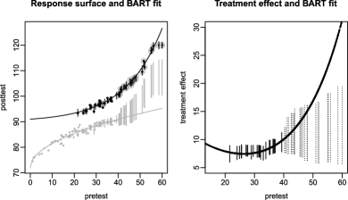
Figure 1: Left panel: simulated data (points) and true response surfaces. The black upper curve and points that follow it correspond to the treatment condition; the grey lower curve and points that follow it correspond to the control condition. BART inference for each treated observation is displayed as a 95% posterior interval for $f(1,x_{i})$ and $f(0,x_{i})$. Discarded units (described in Section 4) are circled. Right panel: solid curve represents the treatment effect as it varies with our pretest, $X$. BART inference is displayed as 95% posterior intervals for the treatment effect for each treated unit. Intervals for discarded units (described in Section 4) are displayed as dotted lines. In this sample the conditional average treatment effect for the treated (CATT) is 12.2, and the sample average treatment effect for the treated (SATT) is 11.8.

Figure 1 displays simulated data from each of two treatment groups from a hypothetical educational intervention. The 120 observations were generated independently as follows. We generate the treatment variable as $Z\sim\operatorname{Bernoulli}(0.5)$. We generate a pretest measure as $X\mid Z=1\sim\mathrm{N}(40,10^{2})$ and $X\mid Z=0\sim\mathrm{N}(20,10^{2})$. Our post-test potential outcomes are drawn as $Y(0)\mid X\sim\mathrm{N}(72+3\sqrt{X},1)$ and $Y(1)\mid X\sim\mathrm{N}(90+\exp(0.06X),1)$. Since we conceptualize both our confounder and our outcome as test scores, a ceiling is imposed on each (60 and 120, resp.). Even with this constraint this is an extreme example of heterogeneous treatment effects, designed, along with the lack of overlap, to make it extremely difficult for any method to successfully estimate the true treatment effect.

In the left panel, the upper solid black curve represents $E[Y(1)\mid X]$ and the lower grey one $E[Y(0)\mid X]$. The black circles close to the upper curve are the treated and the grey squares close to the lower curve are the untreated (ignore the circled points for now). Since there is only one confounding covariate, $X$, the difference between the two response surfaces at any level of $X$ represents the treatment effect for observations with that value of the pretest $X$. In this sample the conditional average treatment effect for the treated (CATT) is 12.2, and the sample average treatment effect for the treated (SATT) is 11.8.

A linear regression fit to the data yields a substantial underestimate, 7.1 (s.e. 0.62), of both estimands. Propensity score matching (not restricted to common support) with subsequent regression adjustment yields a much better estimate, 10.4 (s.e. 0.52), while the IPTW regression estimate is 9.6 (s.e. 0.45). For both of these methods the propensity scores were estimated using logistic regression.

The left panel of Figure 1 also displays the BART fit to the response surface (with number of trees equal to 100 since there are only 120 observations). Each vertical line segment corresponds to individual level inference about either $E[Y_{i}(0)\mid X_{i}]$ or $E[Y_{i}(1)\mid X_{i}]$ for each treated observation. Note that the fit is quite good until we try to predict $E[Y_{i}(0)\mid X_{i}]$ beyond the support of the data. The right panel displays the true treatment effect as it varies with $X$, $E[Y(1)-Y(0)\mid X]$, as a solid curve. The BART inference (95% posterior interval) for the treatment effect for each treated unit is superimposed as a vertical segment (ignore the solid versus dashed distinction for now). These individual-level inferences can be averaged to obtain inference for the effect of the treatment on the treated which is 9.5 with 95% posterior interval (7.7, 11.8); this interval best corresponds to inference with respect to the conditional average treatment effect on the treated [Hill (2011)].

None of these methods yields a 95% interval that captures CATT. BART is the only method to capture SATT, though at the expense of a wider uncertainty interval. All the approaches are hampered by the fairly severe lack of common support. Notice, however, the way that the BART-generated uncertainty bounds grow much wider in the range where there is no overlap across treatment groups ($X>40$). The marginal intervals nicely cover the true conditional treatment effects until we start to leave this neighborhood. However, inference in this region is based on extrapolation. Our goal is to devise a rule to determine how much “excess” uncertainty should warrant removing a unit from the analysis. We will return to this example in Section 4.

3 Identifying areas of common support

It is typical in causal inference to assume common support. In particular, many researchers assume “strong ignorability” [Rosenbaum and Rubin (1983)] which combines the standard ignorability assumption discussed above with an assumption of common support often formalized as $0<\Pr(Z\mid\mathbf{X})<1$. It is somewhat less common for researchers to check whether common support appears to be empirically satisfied for their particular data set.

Moreover, the definition of common support is itself left vague in practice. Typically, $\mathbf{X}$ comprises the set of covariates the researcher has chosen to justify the ignorabilty assumption. As such, conservative researchers will understandably include a large number of pretreatment variables in $\mathbf{X}$. However, this will likely mean that $\mathbf{X}$ includes any number of variables that are not required to satisfy ignorability once we condition on some other subset of the vector of covariates. Importantly, the requirement of common support need not hold for the variables not in this subset, thus, trying to force common support on these extraneous variables can lead to unnecessarily discarding observations.

The goal instead should be to ensure common causal support which can be defined as $0<\Pr(Z\mid\mathbf{W})<1$, where $\mathbf{W}$ represents any subset of $\mathbf{X}$ that will satisfy $Y(0),Y(1)\perp Z\mid\mathbf{W}$. Because BART takes advantage of the information in the outcome variable, it should be better able to target common causal support as will be demonstrated in the examples below. Propensity score methods, on the other hand, ignore this information, rendering them incapable of making these distinctions.

If the common causal support assumption does not hold for the units in our inferential sample (the units in our sample about whom we’d like to make causal inference), we do not have direct empirical evidence about the counterfactual state for them. Therefore, if we retain these units in our sample, we run the risk of obtaining biased treatment effect estimates.

One approach to this problem is to weight observations by the strength of support [for an example of this strategy in a propensity score setting, see Crump et al. (2009)]. This strategy may yield efficiency gains over simply discarding problematic units. However, this approach has two key disadvantages. First, if there are a large number of covariates, the weights may become unstable. Second, it changes the interpretation of the estimand to something that may have little policy or practical relevance. For instance, suppose the units that have the most support are those currently receiving the program, however, the policy-relevant question is what would happen to those currently not receiving the program. In this case the estimand would give most weight to those participants of least interest from a policy perspective.

Another option is to identify and remove observations in neighborhoods of the covariate space that lack sufficient common causal support. Simply discarding observations deemed problematic is unlikely to lead to an optimal solution. However, this approach has the advantage of greater simplicity and transparency. More work will need to be done, however, to provide strategies for adequately profiling the discarded observations as well as those that we retain for inference; this paper will provide a simple starting point in this effort. The primary goal of this paper is simply to describe a strategy to identify these problematic observations.

3.1 Identifying areas of common causal support with BART

The simple idea is to capitalize on the fact that the posterior standard deviations of the individual-level conditional expectations estimated using BART increase markedly in areas that lack common causal support, as illustrated in Figure 1. The challenge is to determine how extreme these standard deviations should be before we need be concerned. We present several possible rules for discarding units. In all strategies when implementing BART we recommend setting the “number of trees” parameter to 100 to allow BART to better determine the relative importance of the variables.

Recall that the individual-level causal effect for each unit can be expressed as $d_{i}=f(1,\mathbf{x}_{i})-f(0,\mathbf{x}_{i})$. For each unit, $i$, we have explicit information about $f(Z_{i},\mathbf{x}_{i})$. Our concern is whether we have enough information about $f(1-Z_{i},\mathbf{x}_{i})$. The amount of information is reflected in the posterior standard deviations. Therefore, we can create a metric for assessing our uncertainty regarding the sufficiency of the common support for any given unit by comparing $\sigma_{i}^{f_{0}}=\operatorname{sd}(f(0,\mathbf{x}_{i}))$ and $\sigma_{i}^{f_{1}}=\operatorname{sd}(f(1,\mathbf{x}_{i}))$, where $\operatorname{sd}(\cdot)$ denotes the posterior standard deviation. In practice, of course we use Monte Carlo approximations to these quantities, $s_{i}^{f_{0}}$ and $s_{i}^{f_{1}}$, respectively, obtained by calculating the standard deviation of the draws of $f(0,\mathbf{x}_{i})$ and $f(0,\mathbf{x}_{i})$ for the $i$th observation.

BART discarding rules

Our goal is to use the information that BART provides to create a rule for determining which units lack sufficient counterfactual evidence (i.e., residing in a neighborhood without common support). For example, when estimating the effect of the treatment on units, $i$, for which $Z_{i}=a$, one might consider discarding any unit, $i$, with $Z_{i}=a$, for which $s_{i}^{f_{1-a}}>m_{a}$, where $m_{a}=\max_{j}\{s_{j}^{f_{a}}\}$, $\forall j\dvtx Z_{j}=a$. So, for instance, when estimating the effect of the treatment on the treated we would discard treated units whose counterfactual standard deviation $s_{i}^{f_{0}}$ exceeded the maximum standard deviation under the observed treatment condition $s_{i}^{f_{1}}$ across all the treated units.

This cutoff is likely too sharp, however, as even chance disturbances might put some units beyond this threshold. Therefore, a more useful rule might use a cutoff that includes a “buffer” such that we would only discard for unit $i$ in the inferential group defined as those with $Z_{i}=a$, if

$$s_{i}^{f_{1-a}}>m_{a}+\operatorname{sd}\bigl{(}s_{j}^{f_{a}}\bigr{)}\qquad\mbox{({1 sd rule})},$$

where $\operatorname{sd}(s_{j}^{f_{a}})$ represents the estimated standard deviation of the empirical distribution of $s_{j}^{f_{a}}$ over all units with $Z_{j}=a$. For this rule to be most useful, we need $\operatorname{Var}(Y\mid\mathbf{X},Z=0)=\operatorname{Var}(Y\mid\mathbf{X},Z=1)$ to hold at least approximately.

Another option is to consider the squared ratio of posterior standard deviations (or, equivalently, the ratio of posterior variances) for each observation, with the counterfactual posterior standard deviation in the numerator. An approximate benchmark distribution for this ratio might be a $\chi^{2}$ distribution with 1 degree of freedom. Thus, for an observation with $Z_{i}=a$ we can choose cutoffs that correspond to a specified $p$-value of rejecting the hypothesis that the variances are the same of 0.10,

$$\bigl{(}s_{i}^{f_{1-a}}/s_{i}^{f_{a}}\bigr{)}^{2}>2.706\qquad\forall i\dvtx z_{i}=1\mbox{ ({$\alpha=0.10$ rule})}$$

or a $p$-value of 0.05,

$$\bigl{(}s_{i}^{f_{1-a}}/s_{i}^{f_{a}}\bigr{)}^{2}>3.841\qquad\forall i\dvtx z_{i}=1\mbox{ ({$\alpha=0.05$ rule})}.$$

These ratio rules do not require the same type of homogeneity of variance assumption across units as does the 1 sd rule. However, they rest instead on an implicit assumption of homogeneity of variance within unit across treatment conditions. Additionally, they may be less stable and will be prone to rejection for units that have particularly large amounts of information for the observed state. For instance, an observation in a neighborhood of the covariate space that has control units may still reject (i.e., be flagged as a discard) if there are, relatively speaking, many more treated units in this neighborhood as well.

Exploratory analyses using measures of common causal support uncertainty

Another way to make use of the information in the posterior standard deviations is more exploratory. The idea here is to use a classification strategy such as a regression tree to identify neighborhoods of the covariate space with relatively high levels of common support uncertainty. For instance, when the goal is estimation of the effect of the treatment on the treated we may want to determine neighborhoods that have clusters of units with relatively high levels of $s_{i}^{f_{1-Z_{i}}}$ or $s_{i}^{f_{1-Z_{i}}}/s_{i}^{f_{Z_{i}}}$. Then these “flags” combined with researcher knowledge of the substantive context of the research problem can be combined to identify observations or neighborhoods to be excised from the analysis if it is deemed necessary. This approach may have the advantage of being more closely tied to the science of the question being addressed. We illustrate possibilities for exploring and characterizing these neighborhoods in Sections 4.3 and 6.

Reliance on this type of exploratory strategy will likely be eschewed by researchers who favor strict analysis protocols as a means of promoting honesty in research. In fact, the original BART causal analysis strategy was conceived with this predilection in mind, which is why (absent the need or desire to address common support issues) the advice given is to run it only once and at the default settings; this minimizes the amount of researcher “interference” [Hill (2011)]. These preferences may still be satisfied, however, by specifying one of the discarding rules above as part of the analysis protocol. For further discussion of this issue see Section 3.3.

3.2 Competing strategies for identifying common support

The primary competitors to our strategy for identification of units that lack sufficient common causal support rely on propensity scores. While there is little advice directly given to the topic of how to use the propensity score to identify observations that lack common support for the included predictors [for a notable exception see Crump et al. (2009)], in practice, most researchers using propensity score strategies first estimate the propensity score and then discard any inferential units that extend beyond the range of the propensity score [Heckman, Ichimura and Todd (1997), Dehejia and Wahba (1999), Morgan and Harding (2006)]. This type of exclusion is performed automatically in at least two popular propensity score matching software packages, MatchIt in R [Ho et al. (2013)] and psmatch2 in Stata [Leuven and Sianesi (2011)] when the “common support” option is chosen. For instance, if the focus is on the effect of the treatment on the treated, one would typically discard the treated units with propensity scores greater than the maximum control propensity score, unless there happened to be some treated with propensity scores less than the minimum control propensity score (in which case these treated units would be discarded as well).

More complicated caliper matching methods might further discard inferential units that lie within the range of propensity scores of their comparison group if such units are more than a set distance (in propensity score units) away from their closest match [see, e.g., Frolich (2004)]. Given the number of different radius/caliper matching methods and the lack of clarity about the optimal caliper width, it was beyond the scope of this paper to examine those strategies as well.

Weighting methods are typically not coupled with discarding rules since one of the advantages touted by weighting advocates is that IPTW allows the researcher to include their full sample of inferential and comparison units. However, in some situations failure to discard inferential units that are quite different from the bulk of the comparison units can lead to more unstable weight estimates.

We have two primary concerns about use of propensity scores to identify units that fail to satisfy common causal support. First, they require a correct specification of the propensity score model. Offsetting this concern is the fact that our BART strategy requires a reasonably good fit to the response surface. As demonstrated in Hill (2011), however, BART appears to be flexible enough to perform well in this respect even with highly nonlinear and nonparallel response surfaces. A further caveat to this concern is the fact that several flexible estimation strategies have recently been proposed for estimating the propensity score. In particular, Generalized Boosted Models (GBM) and Generalized Additive Models (GAM) have both been advocated in this capacity with mostly positive results [McCaffrey, Ridgeway and Morral (2004), Woo, Reiter and Karr (2008)], although some more mixed findings exist for GBM in particular settings [Hill, Weiss and Zhai (2013)]. In Section 5 we explore the relative performance of these approaches against our BART approach.

Our second concern is that the propensity score strategies ignore the information about common support embedded in the response variable. This can be important because the researcher typically never knows which of the covariates in her data set are actually confounders; if a covariate is not associated with both the treatment assignment and the outcome, we need not worry about forcing overlap with regard to it. Using propensity scores to determine common support gives greatest weight to those variables that are most predictive of the treatment variable. However, these variables may not be most important for predicting the outcome. In fact, there is no guarantee that they are predictive of the outcome variable at all. Conversely, the propensity score may give insufficient weight to variables that are highly predictive of the outcome and thus may underestimate the risk of retaining units with questionable support with regard to such a variable.

The BART approach, on the other hand, naturally and coherently incorporates all of this information. For instance, if there is lack of common support with respect to a variable that is not strongly predictive of the outcome, then the posterior standard deviation for the counterfactual unit should not be systematically higher to a large degree. However, a variable that similarly lacks common support but is strongly predictive of the outcome should yield strong differences in the distributions of the posterior standard deviations across counterfactuals. Simply put, the standard deviations should pick up “important” departures from complete overlap and should largely ignore “unimportant” departures. This ability of BART to capitalize on information in the outcome variable allows it to more naturally target common causal support.

3.3 Honesty

Advocates of propensity score strategies sometimes directly advocate for ignoring the information in the response variable [Rubin (2002)]. The argument goes that such practice allows the researcher to be more honest because a propensity score model can in theory be chosen (through balance checks) before the outcome variable is even included in the analysis. This approach can avoid the potential problem of repeatedly tweaking a model until the treatment effect meets one’s prior expectations. However, in reality there is nothing to stop a researcher from estimating a treatment effect every time he fits a new propensity score model and, in practice, this surely happens. We argue that a better way to achieve this type of honesty is to fit just one model and use a prespecified discarding rule, as can be achieved in the BART approach to causal inference.

4 Illustrative examples

We illustrate some of the key properties of our method using several simple examples. Each example represents just one draw from the given data generating mechanism, thus, these examples are not meant to provide conclusive evidence regarding relative performance of the methods in each scenario. These examples provide an opportunity to visualize some of the basic properties of the BART strategy relative to more traditional propensity score strategies: propensity score matching with regression adjustment and IPTW regression estimates. Since we estimate average treatment effects for the treated in all the examples, for the IPTW approach the treated units all receive weights of 1 and the control units receive weights of $\hat{e}(x)/(1-\hat{e}(x))$, where $\hat{e}(x)$ denotes the estimated propensity score.

4.1 Simple example with one predictor

First, we return to the simple example from Section 2 to see how our common causal support identification strategies work in that setting. Since there is only one predictor and it is a true confounder, common support and common causal support are equivalent in this example and we would not expect to see much difference between the methods.

The circled treated observations in the left-hand panel of Figure 1 indicate the 29 observations that would be dropped using the standard propensity score discard rule. Similarly, the dotted line segments in the right panel of the figure indicate individual-specific treatment effects that would no longer be included in our average treatment effect inference. All three BART discard rules lead to the same set of discarded observations as the propensity score strategy in this example.

SATT and CATT for the remaining units are 7.9 and 8.0, respectively. Our new BART estimate is 8.2 with 95% posterior interval (7.7, 9.0). With this reduced sample propensity score, matching (with subsequent regression adjustment) yields an estimate of the treatment effect at 8.3 (s.e. 0.26) while IPTW yields an estimate of 7.6 (s.e. 0.32).

Advantages of BART over the propensity score approach are not evident in this simple example. They should manifest in examples where the assignment mechanism is more difficult to model or when there are multiple potential confounders and not all variables that predict treatment also predict the outcome (or they do so with different emphasis). We explore these issues next.

4.2 Illustrative examples with two predictors

We now describe twoslightly more complicated examples to illustrate the potential advantages of BART over propensity-score-based competitors. In both examples there are two independent covariates, each generated as $\mathrm{N}(0,1)$, and the goal is to estimate CATT which is equal to 1 (in fact, the treatment effect is constant across observations in these examples). The question in each case is whether some of the treated observations should be dropped due to lack of empirical counterfactuals.

4.2.1 Example 2A: Two predictors, no confounders

In the first example the assignment mechanism is simple—after generating $Z$ as a random flip of the coin, all controls with $X_{1}>0$ are removed. The response surface is generated as $E[Y\mid Z,X_{1},X_{2}]=Z+X_{2}+X_{2}^{2}$, thus, the true treatment effect is constant at 1. Since there are no true confounders in this example, the requirement of common support on both $X_{1}$ and $X_{2}$ will be overly conservative; overlap on neither is required to satisfy common causal support. Figure 2 illustrates how each strategy performs in this scenario.

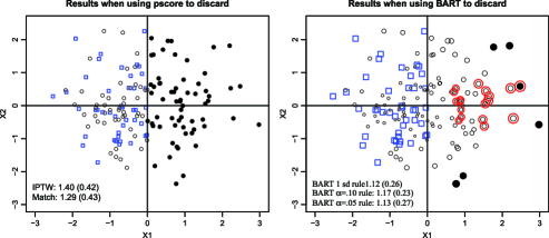
Figure 2: Plots of simulated data with two predictors; the true treatment effect is 1. $X_{1}$ predicts treatment assignment only and $X_{2}$ predicts outcome only. Control observations are displayed as squares. Treated observations are displayed as circles. The left panel displays results based on propensity score common support; solid circles indicate which observations were discarded. In the right panel the size of the circle is proportional to the $s_{i}^{f_{0}}$. Observations discarded based on the BART 1 sd rule are displayed as solid circles. Observations discarded based on the BART $\alpha=0.10$ rule are circled. No observations were discarded based on the BART $\alpha=0.05$ rule ratio rule.

In both plots circles represent treated observations and squares represent control observations. The left panel shows the results based on discarding units that lack common support with respect to the propensity score. The observations discarded by the propensity score method are displayed as solid circles. Since treatment assignment is driven solely by $X_{1}$, there is a close mapping between $X_{1}$ and the propensity score (were it not for the fact that $X_{2}$ was also in the estimation model for the propensity score, the correspondence would be one-to-one). 62 of the 112 treatment observations are dropped based on lack of overlap with regard to the propensity score.

After re-estimating the propensity score matching on the smaller sample, the matching estimate is 1.29. Since treatment assignment is independent of the potential outcomes by design, this estimate should be unbiased over repeated samples. However, it now has less than half the observations available for estimation. Inverse-probability-of-treatment weighting (IPTW) yields an estimate of 1.40 (s.e. 0.42) after discarding.

In the right plot of Figure 2 the size of the circle for each treated unit is proportional to the corresponding size of the posterior standard deviation of the expected outcome under the control condition (in this case, the counterfactual condition for the treated). The size of the square that represents each control observation is proportional to the cutoff level for discarding units. Observations discarded by the 1 sd rule have been made solid. Observations discarded by the $\alpha=0.10$ rule have been circled. No observations were discarded using the $\alpha=0.05$ rule.

In contrast to the propensity score discard rule, the BART 1 sd rule recognizes that $X_{1}$ does not play an important role in the response surface, so it only drops 7 observations that are at the boundary of the covariate space. The corresponding BART estimate is 1.12 with a posterior standard deviation (0.26) that is quite a bit smaller than the standard errors of both propensity score strategies. The $\alpha=0.10$ rule drops 18 observations, on the other hand, and these observations are in a different neighborhood than those dropped by the 1 sd rule since the individual level ratios can get large not just when $s_{i}^{f_{0}}$ is (relatively) large but also when $s_{i}^{f_{1}}$ is (relatively) small. The corresponding estimate of 1.17 and associated standard error (0.23) are quite similar to those achieved by the 1 sd rule. The BART $\alpha=0.05$ rule yields an estimate from the full sample since it leads to no discards (1.13 with a standard error of 0.27). All of the BART strategies benefit from being able to take advantage of the information in the outcome variable.

4.2.2 Example 2B: Two predictors, changing information

In the second example the assignment mechanism is slightly more complicated. We start by generating $Z$ as a binomial draw with probabilities equal to the inverse logit of $X_{1}+X_{2}-0.5X_{1}X_{2}$. Next all control units with $X_{1}>0$ and $X_{2}>0$ are removed. Two different response surfaces are generated, each as $\mathrm{E}[Y\mid Z,X_{1},X_{2}]=Z+0.5X_{1}+2X_{2}+\phi X_{1}X_{2}$, where one version sets $\phi$ to 1 and the other sets $\phi$ to 3. Therefore, both covariates are confounders in this example and both the common support assumption and the common causal support assumption are in question. Once again the treatment effect is 1.

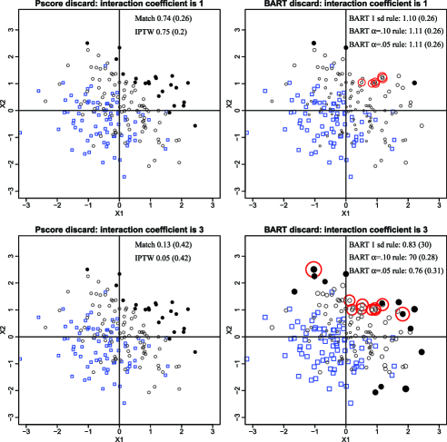
Figure 3: Plots of simulated data with two predictors; the true treatment effect is 1. The display is analogous to Figure 2, although here the two left plots display propensity score results across the two scenarios and the two right display BART results across the two scenarios.

The propensity score discard strategy chooses the same observations to discard across both response surface scenarios because it only takes into account information in the assignment mechanism. Thus, the left panel in Figure 3 presents the same plot twice; the only differences are the estimates of the treatment effect which vary with response surface. The matching estimates get worse (0.74, then 0.13) as the response surface becomes more highly nonlinear as do the IPTW estimates (0.75, then 0.05). The uncertainty associated with the estimates grows between the first and second response surface (from roughly 0.2 to roughly 0.4), yet standard 95% confidence intervals do not cover the truth in the second setting.

The BART discard strategies, on the other hand, respond to information in the response surface. Since the lack of overlap occurs in an area defined by the intersection of $X_{1}$ and $X_{2}$, uncertainty in the posterior counterfactual predictions increases sharply when the coefficient on the interaction moves from 1 to 3 (as displayed in the top and bottom plots in the right panel of Figure 3, resp.) and more observations are dropped for both the 1 sd rule and $\alpha=0.10$ rule. In this example $\alpha=0.10$ rule once again focuses more on observations in the quadrant with lack of overlap with respect to the treatment condition, whereas 1 sd rule identifies observations than tend to have greater uncertainty more generally. No observations are dropped by $\alpha=0.05$ rule even when $\phi$ is 3.

The BART treatment effect estimates in both the first scenario (all about 1.1) and the second scenario (0.83, 0.70 and 0.76) are all closer to the truth than the propensity-score-based estimates in this example. In the first scenario the uncertainty estimates (posterior standard errors of 0.26 for each) are slightly higher than the standard errors for the propensity score estimates; in the second scenario the uncertainty estimates (posterior standard errors all around 0.3) are all smaller than the standard errors for the propensity score estimates.

4.3 Profiling the discarded units: Finding a needle in a haystack

When treatment effects are not homogeneous, discarding observations from the inferential group can change the target estimand. For instance, if focus is on the effect of the treatment on the treated (e.g., CATT or SATT) and we discard treated observations, then we can only make inferences about the treated units that remain (or the population they represent). It is important to have a sense of how this new estimand differs from the original. In this section we illustrate a simple way to “profile” the units that remain in the inferential sample versus those that were discarded in an attempt to achieve common support.

In this example there are 600 observations and 40 predictors, all generated as $\mathrm{N}(1,1)$. Treatment was assigned randomly at the outset; control observations were then eliminated from two neighborhoods in this high-dimensional covariate space. The first such neighborhood is defined by $X_{3}>1$ and $X_{4}>1$, the second by $X_{5}>1$ and $X_{6}>1$. The nonlinear nonparallel response surface is generated as $E[Y(0)\mid\mathbf{X}]<-0.5X_{1}+2X_{2}+0.5X_{5}+2X_{6}+X_{5}X_{6}+0.5X_{5}^{2}+1.5X_{6}^{2}$ and $E[Y(1)\mid\mathbf{X}]<-0.5X_{1}+2X_{2}+0.5X_{5}+2X_{6}+0.2X_{5}X_{6}$. The treatment effect thus varies across levels of the included covariates. Importantly, since $X_{3}$ and $X_{4}$ do not enter into the response surface, only the second of the two neighborhoods that lack overlap should be of concern.

The leftmost plot in Figure 4 displays results from the BART and propensity score methods both before and after discarding. The numbers at the right represent the percentage of the treated observations that were dropped for each discard method. Solid squares represent the true estimand (SATT) for the sample corresponding to that estimate (the same for all methods that do not discard but different for those that do). Circles and line segments represent estimates and corresponding 95% intervals for each estimate. None of the methods that fail to discard has a 95% interval that covers the truth for the full sample. After discarding using the BART rules, all of the intervals cover the true treatment effect for the remaining sample. The propensity score methods drop far fewer treated observations, leading to estimands that do not change much and estimates that still do not cover the estimands for the remaining sample.

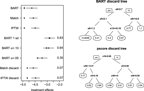
Figure 4: Left plot displays estimands (squares) and attempted inference (circles for estimates and bars for 95% intervals) for the BART and propensity score methods both with and without discarding. The right plots display regression tree fits using the covariates as predictors. The responses used are the statistic from 1 sd rule and then the propensity score, respectively.

We make use of simple regression trees [CART; Breiman et al. (1984), Breiman (2001)] to investigate the differences between the neighborhoods perceived as problematic for each method. Regression trees use predictors to partition the sample into subsamples that are relatively homogenous with respect to the response variable. For our purposes, the predictors are our potential confounders and the response is the statistic corresponding to a given discard rule. A simple tree fit provides a crude means of describing the neighborhoods of the covariate space considered most problematic by each rule with respect to common support. Each tree is restricted to a maximum depth of three for the sake of parsimony.

To profile the units that the BART 1 sd rule considers problematic, we use for the response variable in the tree the corresponding statistic relative to the cutoff rule (appropriate for estimating the effect of the treatment on the treated), $s_{i}^{f_{0}}-m_{1}-\operatorname{sd}(s_{j}^{f_{1}})$, where $i$ and $j$ index treated units. The tree fit is displayed in the top right plot of Figure 4 with the mean of the response in each terminal node given in the corresponding oval. Note that the decision rules for the tree are based almost exclusively on the variables $X_{5}$ and $X_{6}$, as we would hope they would be given how the data were generated.

The tree fit using the propensity score as the response is displayed in the lower right plot of Figure 4. $X_{5}$ plays a far less prominent role in this tree and $X_{6}$ does not appear at all. $X_{16}$, $X_{36}$, and $X_{40}$ play important roles even though these variables are not strong predictors in the response surface; in fact, these are all independent of both the treatment and the response.

This example illustrates two things. First, regression trees may be a useful strategy for profiling which neighborhoods each method has identified as problematic with regard to common support. Second, the propensity score approach may fail to appropriately discover areas that lack overlap if the model for the assignment mechanism and the model for the response surface are not well aligned with respect to the relative importance of each variable. We explore the importance of this type of alignment in more detail in the next section.

5 Simulation evidence

This section explores simulation evidence regarding the performance of our proposed method for identifying lack of common support relative to the performance of two commonly-used and several less-commonly-used propensity-score-based alternatives. Overall we compare the performance of 12 different estimation strategies across 32 different simulated scenarios.

5.1 Simulation scenarios

These scenarios represent all combinations of five design factors. The first factor varies whether the logit of the conditional expectation of the treatment assignment is linear or nonlinear in the covariates. The second factor varies the relative importance of the covariates with regard to the assignment mechanism versus the response surface. In one setting of this factor (“aligned”) there is substantial alignment in the predictive strength of the covariates across these two mechanisms—the covariates that best predict the treatment also predict the outcome well. In the other setting (“not as aligned”) the covariates that best predict the treatment strongly and those that predict the response strongly are less well aligned (for details see the description of the treatment assignment mechanisms and response surfaces and Table 1, below). The third factor is the ratio of treated to control (4:1 or 1:4) units. The fourth factor is the number of predictors available to the researcher (10 versus 50, although in both cases only 8 are relevant). The fifth and final factor is whether or not the nonlinear response surfaces are parallel across treatment and control groups; nonparallel response surfaces imply heterogeneous treatment effects.

In all scenarios each covariate is generated independently from $X_{j}\sim\mbox{N}(0,1)$. These column vectors comprise the matrix $\mathbf{X}$. The general form of the linear treatment assignment mechanism is $Z\sim\operatorname{Binomial}(n,p)$ with $p=\operatorname{logit}^{-1}(\omega+\mathbf{X}\gamma^{L})$, where the offset $\omega$ is specified to create the appropriate ratio of treated to control units. The nonlinear form of this assignment mechanism simply includes some nonlinear transformations of the covariates in $\mathbf{X}$, denoted as $\mathbf{Q}$ with corresponding coefficients $\gamma^{\mathrm{NL}}$. The nonzero coefficients for the terms in these models are displayed in Table 1.

We simulate two distinct sets of response surfaces that differ in both their level of alignment with the assignment mechanism and whether they are parallel. Both sets used are nonlinear in the covariates and each set is generated generally as

$$\mathrm{E}\bigl{[}Y(0)\mid\mathbf{X}\bigr{]} = \mathrm{N}\bigl{(}\mathbf{X}\beta^{\mathrm{L}}_{0}+\mathbf{Q}\beta^{\mathrm{NL}}_{0},1\bigr{)},$$

$$\mathrm{E}\bigl{[}Y(1)\mid\mathbf{X}\bigr{]} = \mathrm{N}\bigl{(}\mathbf{X}\beta^{\mathrm{L}}_{1}+\mathbf{Q}\beta^{\mathrm{NL}}_{1}+\tau,1\bigr{)},$$

where $\beta^{\mathrm{L}}_{z}$ is a vector of coefficients for the untransformed versions of the predictors $\mathbf{X}$ and $\beta^{\mathrm{NL}}_{z}$ is a vector of coefficients for the transformed versions of the predictors captured in $\mathbf{Q}$. In the scenarios with parallel response surfaces, $\tau$ (the constant treatment effect) is 4, $\beta^{\mathrm{L}}_{0}=\beta^{\mathrm{L}}_{1}$, and $\beta^{\mathrm{NL}}_{0}=\beta^{\mathrm{NL}}_{1}$ and both use the coefficients from $Y(0)$ in Table 1 (only nonzero coefficients displayed). In the scenarios with responses surfaces are not parallel, $\tau=0$, and the nonzero coefficients in the $\beta^{\mathrm{L}}_{z}$ and $\beta^{\mathrm{NL}}_{z}$ are displayed in Table 1.

= $\bolds{x_{1}}$ $\bolds{x_{2}}$ $\bolds{x_{1}^{2}}$ $\bolds{x_{2}^{2}}$ $\bolds{x_{2}x_{6}}$ $\bolds{x_{5}}$ $\bolds{x_{6}}$ $\bolds{x_{7}}$ $\bolds{x_{8}}$ $\bolds{x_{9}}$ $\bolds{x_{10}}$ $\bolds{x_{5}^{2}}$ $\bolds{x_{6}^{2}}$ $\bolds{x_{5}x_{6}}$ $\bolds{x_{5}x_{6}x_{7}}$ $\bolds{x_{7}^{2}}$ $\bolds{x_{7}^{3}}$ $\bolds{x_{8}^{2}}$ $\bolds{x_{7}x_{8}}$ $\bolds{x_{9}^{2}}$ $\bolds{x_{9}x_{10}}$ Treatment assignment mechanisms Linear 0.4 $0.2$ $0.4$ 0.2 0.4 $0.4$ Nonlinear 0.4 $0.2$ $0.4$ 0.2 0.4 $0.4$ 0.8 0.8 0.5 0.3 0.8 0.2 0.4 0.3 0.8 0.5 Response surfaces, nonlinear and not parallel Aligned $Y(0)$ 0.5 $2$ 0.5 $2$ 0.4 0.8 0.5 0.5 0.5 0.7 $Y(1)$ 0.5 $1$ 0.5 $0.8$ 0.3 Not as aligned $Y(0)$ 0.5 2.0 0.4 0.5 1 0.5 $2$ 0.5 1.5 0.7 $Y(1)$ 0.5 0.5 0.5 $2$ 0.3

Table 1: Nonzero coefficients in $\gamma^{\mathrm{L}}$ and $\gamma^{\mathrm{L}}$ for the treatment assignment mechanism as well as for $\beta^{\mathrm{L}}_{z}$ and $\beta^{\mathrm{NL}}_{z}$ for the nonlinear, not parallel response surfaces. Coefficients for the parallel response surface are the same as those for $Y(0)$ in the nonparallel response surface

Table 1 helps us understand the alignment in predictor strength between the assignment mechanism and response surfaces for each of the two scenarios. The “aligned” version of the response surfaces places weight on the covariates most predictive of the assignment mechanism (both the linear and nonlinear pieces). There is no reason to believe that this alignment occurs in real examples. Therefore, we explore a more realistic scenario where coefficient strength is “not as aligned.”

We replicate each of the 32 scenarios 200 times and in each simulation run we implement each of 12 different modeling strategies. For each the goal is to estimate the conditional average effect of the treatment on the subset of treated units that were not discarded.

5.2 Estimation strategies compared

We compare three basic causal inference strategies without discarding—BART [implemented as described above and in Hill (2011) except using 100 trees], propensity score matching, and IPTW—with nine strategies that involve discarding.

The first three discarding approaches discard using the 1 sd rule, the $\alpha=0.10$ rule, and the $\alpha=0.05$ rule and each is coupled with a BART analysis of the causal effect on the remaining sample. The remaining 6 approaches are combinations of 3 propensity score discarding strategies and 2 analysis strategies. The 3 propensity score discard strategies vary by the estimation strategy for the propensity score model: standard logit, generalized boosted regression model [recommended for propensity score estimation by McCaffrey, Ridgeway and Morral (2004)], and generalized additive models [recommended for propensity score estimation by Woo, Reiter and Karr (2008)]. The 2 analysis strategies (each conditional on a given propensity score estimation model) are one-to-one matching (followed by regression adjustment) and inverse-probability of treatment weighting (in the context of a linear regression model). In all propensity score strategies the propensity score is re-estimated after the initial units are discarded. The $y$-axis labels of the results figures indicate these 12 different combinations of strategies. All strategies estimate the effect of the treatment on the treated.

We implement these models in several packages in R [R Core Team (2012)]. We use the bart() function in the BayesTree package [Chipman and McCulloch (2009)] to fit BART models. For each BART fit, we allow the maximum number of trees in the sum to be 100 as described in Section 3.1 above. To ensure the convergence of the MCMC in BART without having to check for each simulation run, we are conservative and let the algorithm run for 3500 iterations with the first 500 considered burn-in. To implement the GBM routine, we use the gbm() function of the gbm package [Ridgeway (2007)]. In an attempt to optimize the settings for esimating propensity scores, we adopt the suggestions of [McCaffrey, Ridgeway and Morral (2004), 409] for the tuning parameters of the GBM: $100$ trees, a maximum of 4 splits for each tree, a small shrinkage value of $0.0005$, and a random sample of 50% of the data set to be use for each fit in each iteration. We use the gam() function of the gam package [Hastie (2009)] to implement the GAM routine.

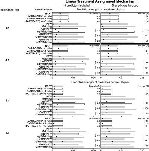
Figure 5: Simulation results for the scenarios in which the treatment assignment is linear and the response surfaces are parallel. Solid dots represent average differences between estimated treatment effects and the true ones standardized by the standard deviations of the outcomes. Bars are root mean square errors (RMSE) of such estimates. The drop rates are the percentage discarded units. Discard and analysis strategies are described in the text. Five modeling strategies are highlighted with hollow bars for comparison: the three BART strategies and the most likely propensity scores versions to be implemented (these are the same strategies illustrated in the examples in Section 4).

5.3 Simulation results

Figure 5 presents results from 8 scenarios that have the common elements of a linear treatment assignment mechanism and parallel response surfaces. The linear treatment assignment mechanism should favor the propensity score approaches. The top panel of 4 plots in this figure corresponds to the setting where there is alignment in the predictive strength of the covariates; this setting should favor the propensity score approach as well since it implicitly uses information about the predictive strength of the covariates with regard to the treatment assignment mechanism to gauge the importance of each covariate as a confounder. The bottom panel of Figure 5 reflects scenarios in which the predictive strength of the covariates is not as well aligned between the treatment assignment mechanism and the response surface. This setup provides less of an advantage for the propensity score methods. The potential for bias across all methods, however, should be reduced.

Within each plot, each bar represents the root mean square error (RMSE) of the estimates for that scenario for a particular estimation strategy. The dots represent the absolute bias (the absolute value of the average difference between the estimates and the CATT estimand). Drop rates for the discarding methods are indicated on the right-hand side of each plot. We highlight (with unfilled bars) the BART discard/analysis strategies as well as the two propensity score discard strategies that rely on the logit specification of the propensity score model (the most commonly used model for estimating propensity scores).

The first thing to note about Figure 5 is that there is little bias in any of the methods across all of these eight scenarios and likewise the RMSEs are all small. Within this we do see some small differences in the absolute levels of bias across methods in the aligned scenarios, with slightly less bias evidenced by the propensity score approaches and smaller RMSEs for the BART approaches. In the nonaligned scenarios the differences in bias nearly disappear (with a slight advantage overall for BART) and the advantage with regard to RMSE becomes slightly more pronounced. None of the methods drop a large percentage of treated observations, but the BART rules discard the least (with one small exception).

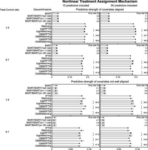
Figure 6: Simulation results for the scenarios with nonlinear treatment assignment and parallel response surfaces. Description otherwise the same as in Figure 5.

The eight plots in Figure 6 represent scenarios in which the nonlinear treatment assignment mechanism was paired with parallel response surfaces. The nonlinear treatment assignment presents a challenge to the naively specified propensity score models. These plots vary between upper and lower panels in similar ways as seen in Figure 5. Overall, these plots show substantial differences in results between the BART and propensity score methods. The BART discard methods drop far fewer observations and yield substantially less bias and smaller RMSE across the board. The differences between propensity score methods are negligible.

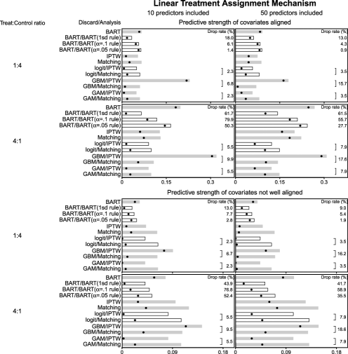
Figure 7: Simulation results for the scenarios with nonlinear treatment assignment and nonparallel response surfaces. Description otherwise the same as in Figure 5.

Figure 7 corresponds to scenarios with linear treatment assignment mechanism and nonparallel response surfaces. The top panel shows little difference in RMSE or bias for the BART 1 sd rule compared to the best propensity score strategies (sometimes slightly better and sometimes slightly worse). The BART $\alpha=0.10$ rule and $\alpha=0.05$ rule perform slightly worse than the 1 sd rule in all four scenarios. The bottom panel of Figure 7 shows slightly more clear gains with regard to RMSE for the BART discard methods; the results regarding bias, however, are slightly more mixed, though the differences are not large. Across all scenarios the BART 1 sd rule drops a higher percentage of treated observations than the propensity score rules; this difference is substantial in the scenarios where treated outnumber controls 4 to 1. The BART 1 sd rule always drops more than the ratio rules when controls outnumber treated but not when the treated outnumber controls.

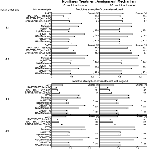
Figure 8: Simulation results for the scenarios with nonlinear treatment assignment and nonparallel response surfaces. Description otherwise the same as in Figure 5.

The eight plots in Figure 8 all represent scenarios with nonlinear treatment assignment mechanism and nonparallel response surfaces. In the top panel the differences between the BART methods and the best propensity score methods are not large with regard to either bias or RMSE with BART performing worst in the scenario with 50 potential predictors and more treated than controls. In the bottom plots corresponding to misaligned strength of coefficients BART displays consistent gains over the propensity scores approaches both in terms of bias and RMSE. All the methods discard a relatively high percentage of treated observations.

While it does not dominate at every combination of our design factors, the BART 1 sd rule appears to perform most reliably across all the methods overall. In particular, it almost always performs better with regard to RMSE and it often performs well with respect to bias as well.

6 Discarding and profiling when examining the effect of breastfeeding on intelligence

The putative effect of breastfeeding on intelligence or cognitive achievement has been heavily debated over the past few decades. This debate is complicated by the fact that this question does not lend itself to direct experimentation and, thus, the vast majority of the research that has been performed has relied on observational data. While many of these studies demonstrate small to medium-sized positive effects [see, e.g., Anderson, Johnstone and Remley (1999), Mortensen et al. (2002), Lawlor et al. (2006), among others] some contrary evidence exists [notably Drane and Logemann (2000), Jain, Concato and Leventhal (2002), Der, Batty and Deary (2006)]. It has been hypothesized that the effects of breastfeeding increase with the length of exposure, therefore, to maximize the chance of detecting an effect, it makes sense to examine the effect of breastfeeding for extended durations versus not at all. This approach is complicated by the fact that mothers who breastfeed for longer periods of time tend to have substantially different characteristics on average than those who never breastfeed (as an example see the unmatched differences in means in Figure 9). Thus, identification of areas of common support should be an important characteristic of any analysis attempting to identify such effects.

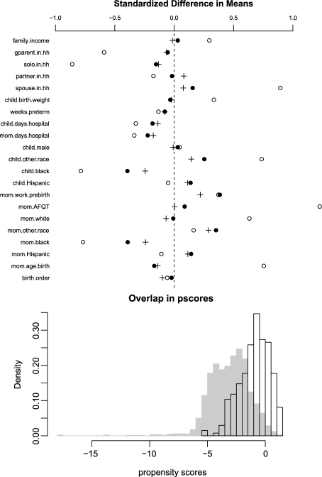
Figure 9: Top panel: balance represented as standardized differences in means for each of three samples: unmatched (open circles), post-discarding matched (solid circles), and post-discarding re-weighted (plus signs). Discarding combined with matching and weighting substantially improve the balance. Bottom panel: overlapping histograms of propensity scores (on the linear scale) for both breastfeeding groups.

Randomized experiments have been performed that address related questions. Such studies have been used to establish a causal link, for instance, between two fatty acids found in breast milk (docosahexaenoic acid and arachidonic acid) and eyesight and motor development [see, e.g., Lundqvist-Persson et al. (2010)]; this could represent a piece of the causal pathway between breastfeeding and subsequent cognitive development. Furthermore, a recent large-scale study [Kramer et al. (2008)] randomized encouragement to breastfeed and found significant, positive estimates of the intention-to-treat effect (i.e., the effect of the randomized encouragement) on verbal and performance IQ measures at six and a half years old. Even a randomized study such as this, however, cannot directly address the effects of prolonged breastfeeding on cognitive outcomes. This estimation would still require comparisons between groups that are not randomly assigned. Moreover, an instrumental variables approach would not necessarily solve the problem either. Binary instruments cannot be used to identify effects at different dosage levels of a treatment without further assumptions. However, dichotomization of breastfeeding duration would almost certainly lead to a violation of the exclusion restriction.

We examine the effect of breastfeeding for 9 months or more (compared to not breastfeeding at all) on child math and reading achievement scores at age 5 or 6. Our “treatment” group consists of 271 mothers who breastfed at least 38 weeks and our “control” group consists of 1832 mothers who reported 0 weeks of breastfeeding. To create a cleaner comparison, we remove from our analysis sample mothers who breastfed greater than 0 weeks or less than 38 weeks. Given that the most salient policy question is whether new mothers should be (more strongly) encouraged to breastfeed their infants, the estimand of interest is the effect of the treatment on the controls. That is, we would like to know what would have happened to the mothers in the sample who were observed to not breastfeed their children if they had instead breastfed for at least 9 months.

We used data from the National Longitudinal Survey of Youth (NLSY) Child Supplement [for more information see Chase-Lansdale et al. (1991)]. The NLSY is a longitudinal survey that began in 1979 with a cohort of approximately 12,600 young men and women aged 14 to 21 and continued annually until 1994 and biannually thereafter. The NLSY started collecting information on the children of female respondents in 1986. Our sample comprises 2103 children of the NLSY born from 1982 to 1993 who had been tested in reading and math at age 5 or 6 by the year 2000 and whose mothers fell into our two breastfeeding categories (no months or 9 plus months).

In addition to information on number of weeks each mother breastfed her child, we also have access to detailed information on potential confounders. The covariates included are similar to those used in other studies on breastfeeding using the NLSY [see, e.g., Der, Batty and Deary (2006)], however, we excluded several post-treatment variables that are often used, such as child care and home environment measures since these could bias causal estimates [Rosenbaum (1984)]. Measurements regarding the child at birth include birth order, race/ethnicity, sex, days in hospital, weeks preterm, and birth weight. Measurements on the mother include her age at the time of birth, race/ethnicity, Armed Forces Qualification Test (AFQT) score, whether she worked before the child was born, days in hospital after birth, and educational level at birth. Household measures include income (at birth), whether a spouse or partner was present at the time of the birth of the child, and whether grandparents were present one year before birth.

The children in the NLSY subsample were tested on a variety of cognitive measures at each survey point (every two years starting with age 3 or 4). We make use of the Peabody Individual Achievement Test (PIAT) math and reading scores from assessments that took place either at age 5 or 6 (depending on the timing of the survey relative to the age of the child).

To allow focus on issues of common support and causal inference and to avoid debate about the best way to deal with the missing data, we simply limit our sample to complete cases. Due to this restriction, this sample should not be considered to be representative of all children in the NLSY child sample whose mothers fell into the categories defined.

Comparing the two groups based on the baseline characteristics reveals imbalance. Figure 9 displays the balance for the unmatched (open circles), post-discarding matched (solid circles), and post-discarding re-weighted (plus signs) samples. The matched and reweighted samples are much more closely balanced than the unmatched sample, particularly for the household and race variables.

The bottom panel of Figure 9 displays the overlap in propensity scores estimated by logistic regression (displayed on the linear scale). The histogram for the control units has been shaded in with grey, while the histogram for the treated units is simply outlined in black. This plot suggests lack of common support for the control units with respect to the estimated propensity score. The question remains, however, whether sufficient common support on relevant covariates exists.

We use both propensity score and BART approaches to address this question. The results of our analyses are summarized in Table 2 which displays for each method and test score (reading or math) combination: treatment effect estimate, standard error, and number of units discarded. Without discarding there is a substantial degree of heterogeneity between BART, linear regression after one-to-one nearest neighbor propensity score matching with replacement (Match), IPTW (propensity scores estimated in all cases using logistic regression), regression and standard linear regression. For reading test scores the treatment effect estimates are (3.5, 2.5, 1.5, and 3.2) with standard errors ranging between roughly 0.9 and 1.6. For math test scores the estimates are (2.4, 3.4, 2.6, and 2.2) with standard errors ranging between roughly 0.9 and 1.9.

Table 2: Table displays treatment effect estimates, associated standard errors, and number of units discarded for each method and test score (reading or math) combination

	Reading			Math
	Treatment	Standard	Number	Treatment	Standard	Number
Method	effect	error	discarded	effect	error	discarded
BART	3.5	1.07	$0$	2.4	1.05	$0$
BART-D1	3.5	1.07	$0$	2.4	1.05	$0$
BART-D2	3.5	1.04	$93$	2.4	1.04	$53$
BART-D3	3.5	1.07	$0$	2.4	1.05	$0$
Match	2.5	1.62	$0$	3.4	1.74	$0$
Match-D	3.6	1.50	$168$	1.5	1.13	$168$
Match-D-RE	3.8	1.43	$168$	1.5	1.18	$168$
IPTW	1.5	1.57	$0$	2.6	1.92	$0$
IPTW-D	1.6	1.52	$168$	2.6	1.85	$168$
IPTW-D-RE	1.6	1.51	$168$	2.6	1.80	$168$
OLS	3.2	0.87	$0$	2.2	0.89	$0$

For the analysis of the effect on reading, the BART $\alpha=0.10$ rule would discard 93 observations, however, neither the BART 1 sd rule or the $\alpha=0.05$ rule would discard any. Regardless of the discard strategy, however, the BART estimate is about 3.5 with posterior standard deviation of a little over 1. Levels of discarding are similar for math test scores, although for this outcome the BART $\alpha=0.10$ rule would discard 53. Similarly, the effect estimates (2.4) and associated uncertainty estimates (a little over 1) are almost identical across strategies.

Using propensity scores (estimated using a logistic model linear in the covariates) to identify common support discards 168 of the control units. This strategy does not change depending on the outcome variable. Using propensity scores estimated on the remaining units, matching (followed by regression adjustment; Match-D-RE) and IPTW regression (IPTW-D-RE) yield reading treatment effect estimates for the reduced sample of 3.8 (s.e. 1.43) and 1.6 (s.e. 1.51), respectively. If we do not re-estimate the propensity score after discarding, these estimates (Match-D and IPTW-D) are 3.6 (s.e. 1.50) and 1.6 (s.e. 1.52), respectively. The results for math are quite heterogeneous as well, with matching and IPTW yielding estimates of 1.5 (s.e. 1.18) and 2.6 (s.e. 1.80), respectively. Re-estimating the propensity scores did not change the results for this outcome (when rounding to the first decimal place).

It is important to remember that the methods that discard units are estimating different estimands than those that do not, therefore, direct comparisons between the BART and propensity score estimates are not particularly informative. Importantly, however, both propensity score methods are estimating the same effect (they discarded the exact same units), therefore, the differences between these estimates are a bit disconcerting. One possible explanation for these discrepancies is that the two propensity score methods do yield somewhat different results with regard to balance as displayed in Figure 9; IPTW yields slightly closer balance on average (though not for every covariate).

What might account for the differences in which units were discarded between the BART and propensity score approaches? To better understand, we more closely examine which variables each strategy identifies as being important with regard to common support by considering the predictive strength of each covariate with regard to both propensity score and BART models in combination with fitting regression trees with the discard statistics as response variables just as in Section 4.3.

BART identifies birth order, mother’s AFQT score, household income, mother’s educational attainment at time of birth, and the number of days the child spent in the hospital as the most important continuous predictors for both outcomes (although the relative importance of each changes a bit between outcomes). Recall, however, that the BART discard rules are driven by circumstances in which the level of information about the outcome changes drastically across observations in different treatment groups. The overlap across treatment groups for most of these variables is actually quite good. While some, like AFQT, are quite imbalanced, overlap still exists for all of the inferential (control) observations. More problematic in terms of common support is the variable that reflects the number of days the child spent in the hospital; 30 children of mothers who did not breastfeed had values for this variable higher than the maximum value (30 days) for the children of mothers who did breastfeed for nine or more months. Not surprisingly, this variable is the primary driving force behind the BART 1 sd rule as seen in Figure 10, particularly for mothers who did not have a spouse living in the household at the time of birth. Mother’s education plays a more important role for the BART ratio rules for the reading outcome. This variable also has some issues with incomplete overlap and it is slightly more important in predicting reading outcomes than math outcomes.

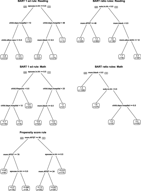
Figure 10: Regression trees explore the characteristics of units at risk of failing to satisfy common (causal) support. The top two trees use the two statistics from the BART discard rules for the reading outcome variable as the response; the next two trees use the two statistics from the BART discard rules for the math outcome variable. The bottom tree uses the estimated propensity score subtracted from the cutoff (maximum estimated propensity score for the controls). The predictors of the trees are all the potential confounding covariates. For all trees the larger the statistic the more likely the unit will be discarded, so focus is on the rightmost part of each tree.

A look at the fitted propensity score model, on the other hand, reveals that breastfeeding for nine or more months is predicted most strongly by the mother’s AFQT scores, her educational attainment, and her age at the time of the birth of her child. Thus, these variables drive the discard rule. In particular, the critical role of mom’s AFQT is evidenced in the regression tree for the discard rule at the bottom of Figure 10. Children whose mothers were not married at birth and whose AFQT scores were less than 50 were most likely to be discarded from the group of nonbreastfeeding mothers about whom we would like to make inferences.

What conclusions can we draw from this example? Substantively, if we feel confident about the ignorability assumption, the BART results suggest a moderate positive impact of breastfeeding 9 or more months on both reading and math outcomes at age 5 or 6. The propensity score results for the sample that remain after discarding for common support are more mixed, with only the matching estimates on reading outcomes showing up as positive and statistically significant.

Methodologically, this is an example in which propensity score rules yield more discards than BART rules. The most reliable rule based on our simulation results (the BART 1 sd rule) would not discard any units. A closer look at the overlap for specific covariates and at regression trees for the discard statistics indicates that the BART discard rules may represent a better reflection of the actual relationships between the variables. The lack of stability of the propensity score estimates is also cause for concern. We emphasize, however, that we have used rather naive propensity score approaches which are not intended to represent best practice. Given the current lack of guidance with regard to optimal choices for propensity score models and specific matching and weighting methods, we chose instead to use implementations that were as straightforward as the BART approach.

7 Discussion

Evaluation of empirical evidence for the common support assumption has been given short shrift in the causal inference literature although the implications can be important. Failure to detect areas that lack common causal support can lead to biased inference due to imbalance or inappropriate model extrapolation. On the other extreme, overly conservative assessment of neighborhoods or units that seem to lack common support may be equally problematic.

This paper distinguishes between the concepts of common support and common causal support. It introduces a new approach for identifying common causal support that relies on Bayesian Additive Regression Trees(BART). We believe that this method’s flexible functional form and its ability to take advantage of information in the response surface allows it to better target areas of common causal support than traditional propensity-score-based methods. We also propose a simple approach to profiling discarded units based on regression trees. The potential usefulness of these strategies has been demonstrated through examples and simulation evidence and the approach has been illustrated in a real example.

While this paper provides some evidence that BART may outperform propensity score methods in the situations tested, we do not claim that it is uniformly superior or that it is the only strategy for incorporating information about the outcome variable. We acknowledge that there are many ways of using propensity scores that we did not test, however, our focus was on examination of methods that were straightforward to implement and do not require complicated interplay between the researcher’s substantive knowledge and the choice of how to implement (what propensity score model to fit, which matching or weighting method to use, which variables to privilege in balancing, which balance statistics to use). We hope that this paper is a starting point for further explorations into better approaches for identifying common support, investigating the role of the outcome variable in causal inference methods, and development of more effective ways of profiling units that we deem to lack common causal support.

There is a connection between this work and that of others [e.g., Brookhart et al. (2006)] who have pointed out the danger of strategies that implicitly assign greater importance to variables that most strongly influence the treatment variable but that may have little or no direct association with the outcome variable. In response, some authors such as Kelcey (2011) have outlined approaches to choosing confounders in ways that make use of the observed association between the possible confounders and the potential outcomes. Another option that is close in spirit to the propensity score techniques but makes use of outcome data (at least in the control group) would be a prognostic score approach [Hansen (2008)]. To date, there has been no formal discussion of use of prognostic cores for this purpose, but this might be a useful avenue for further research.

References

- Anderson, Johnstone and Remley (1999) {barticle}[pbm] \bauthor\bsnmAnderson, \bfnmJ. W.\binitsJ. W., \bauthor\bsnmJohnstone, \bfnmB. M.\binitsB. M. and \bauthor\bsnmRemley, \bfnmD. T.\binitsD. T. (\byear1999). \btitleBreast-feeding and cognitive development: A meta-analysis. \bjournalAm. J. Clin. Nutr. \bvolume70 \bpages525–535. \bidissn=0002-9165, pmid=10500022 \bptokimsref \endbibitem
- Breiman (2001) {barticle}[author] \bauthor\bsnmBreiman, \bfnmL.\binitsL. (\byear2001). \btitleRandom forests. \bjournalMachine Learning \bvolume45 \bpages5–32. \bptokimsref \endbibitem
- Breiman et al. (1984) {bbook}[author] \bauthor\bsnmBreiman, \bfnmL.\binitsL., \bauthor\bsnmFreidman, \bfnmJ. H.\binitsJ. H., \bauthor\bsnmOlshen, \bfnmR. A.\binitsR. A. and \bauthor\bsnmStone, \bfnmC. J.\binitsC. J. (\byear1984). \btitleClassification and Regression Trees. \bpublisherWadsworth, \blocationBelmont, CA. \bptokimsref \endbibitem
- Brookhart et al. (2006) {barticle}[pbm] \bauthor\bsnmBrookhart, \bfnmM. Alan\binitsM. A., \bauthor\bsnmSchneeweiss, \bfnmSebastian\binitsS., \bauthor\bsnmRothman, \bfnmKenneth J.\binitsK. J., \bauthor\bsnmGlynn, \bfnmRobert J.\binitsR. J., \bauthor\bsnmAvorn, \bfnmJerry\binitsJ. and \bauthor\bsnmStürmer, \bfnmTil\binitsT. (\byear2006). \btitleVariable selection for propensity score models. \bjournalAm. J. Epidemiol. \bvolume163 \bpages1149–1156. \biddoi=10.1093/aje/kwj149, issn=0002-9262, mid=NIHMS8838, pii=kwj149, pmcid=1513192, pmid=16624967 \bptokimsref \endbibitem
- Chase-Lansdale et al. (1991) {barticle}[author] \bauthor\bsnmChase-Lansdale, \bfnmP.\binitsP., \bauthor\bsnmMott, \bfnmF. L.\binitsF. L., \bauthor\bsnmBrooks-Gunn, \bfnmJ.\binitsJ. and \bauthor\bsnmPhilips, \bfnmD. A.\binitsD. A. (\byear1991). \btitleChildren of the National Longitudinal Survey of Youth: A unique research opportunity. \bjournalDevelopmental Psychology \bvolume27 \bpages918–931. \bptokimsref \endbibitem
- Chipman, George and McCulloch (2007) {bincollection}[mr] \bauthor\bsnmChipman, \bfnmHugh\binitsH., \bauthor\bsnmGeorge, \bfnmEdward\binitsE. and \bauthor\bsnmMcCulloch, \bfnmRobert\binitsR. (\byear2007). \btitleBayesian ensemble learning. In \bbooktitleAdvances in Neural Information Processing Systems 19 (\beditor\bfnmB.\binitsB. \bsnmSchölkopf, \beditor\bfnmJ.\binitsJ. \bsnmPlatt and \beditor\bfnmT.\binitsT. \bsnmHoffman, eds.). \bpublisherMIT Press, \blocationCambridge, MA. \bptokimsref \endbibitem
- Chipman, George and McCulloch (2010) {barticle}[author] \bauthor\bsnmChipman, \bfnmH. A.\binitsH. A., \bauthor\bsnmGeorge, \bfnmE. I.\binitsE. I. and \bauthor\bsnmMcCulloch, \bfnmR. E.\binitsR. E. (\byear2010). \btitleBART: Bayesian additive regression trees. \bjournalAnn. Appl. Stat. \bvolume4 \bpages266–298. \bptokimsref \endbibitem
- Chipman and McCulloch (2009) {bmisc}[author] \bauthor\bsnmChipman, \bfnmHugh\binitsH. and \bauthor\bsnmMcCulloch, \bfnmRobert\binitsR. (\byear2009). \bhowpublishedBayesTree: Bayesian methods for tree based models. R package version 0.3-1. \bptokimsref \endbibitem
- Crump et al. (2009) {barticle}[mr] \bauthor\bsnmCrump, \bfnmRichard K.\binitsR. K., \bauthor\bsnmHotz, \bfnmV. Joseph\binitsV. J., \bauthor\bsnmImbens, \bfnmGuido W.\binitsG. W. and \bauthor\bsnmMitnik, \bfnmOscar A.\binitsO. A. (\byear2009). \btitleDealing with limited overlap in estimation of average treatment effects. \bjournalBiometrika \bvolume96 \bpages187–199. \biddoi=10.1093/biomet/asn055, issn=0006-3444, mr=2482144 \bptokimsref \endbibitem
- Dehejia and Wahba (1999) {barticle}[author] \bauthor\bsnmDehejia, \bfnmRajeev H.\binitsR. H. and \bauthor\bsnmWahba, \bfnmSadek\binitsS. (\byear1999). \btitleCausal effects in nonexperimental studies: Reevaluating the evaluation of training programs. \bjournalJ. Amer. Statist. Assoc. \bvolume94 \bpages1053–1062. \bptokimsref \endbibitem
- Der, Batty and Deary (2006) {barticle}[author] \bauthor\bsnmDer, \bfnmGeoff\binitsG., \bauthor\bsnmBatty, \bfnmG. David\binitsG. D. and \bauthor\bsnmDeary, \bfnmIan J.\binitsI. J. (\byear2006). \btitleEffect of breast feeding on intelligence in children: Prospective study, sibling pairs analysis, and meta-analysis. \bjournalBritish Medical Journal \bvolume333 \bpages945–950. \bptokimsref \endbibitem
- Drane and Logemann (2000) {barticle}[pbm] \bauthor\bsnmDrane, \bfnmD. L.\binitsD. L. and \bauthor\bsnmLogemann, \bfnmJ. A.\binitsJ. A. (\byear2000). \btitleA critical evaluation of the evidence on the association between type of infant feeding and cognitive development. \bjournalPaediatr. Perinat. Epidemiol. \bvolume14 \bpages349–356. \bidissn=0269-5022, pmid=11101022 \bptokimsref \endbibitem
- Frolich (2004) {barticle}[author] \bauthor\bsnmFrolich, \bfnmM.\binitsM. (\byear2004). \btitleFinite-sample properties of propensity-score matching and weighting estimators. \bjournalThe Review of Economics and Statistics \bvolume86 \bpages77–90. \bptokimsref \endbibitem
- Green and Kern (2012) {barticle}[author] \bauthor\bsnmGreen, \bfnmDonald P.\binitsD. P. and \bauthor\bsnmKern, \bfnmHolger L.\binitsH. L. (\byear2012). \btitleModeling heterogeneous treatment effects in survey experiments with Bayesian additive regression trees. \bjournalPublic Opinion Quarterly \bvolume76 \bpages491–511. \bptokimsref \endbibitem
- Hansen (2008) {barticle}[mr] \bauthor\bsnmHansen, \bfnmBen B.\binitsB. B. (\byear2008). \btitleThe prognostic analogue of the propensity score. \bjournalBiometrika \bvolume95 \bpages481–488. \biddoi=10.1093/biomet/asn004, issn=0006-3444, mr=2521594 \bptokimsref \endbibitem
- Hastie (2009) {bmisc}[author] \bauthor\bsnmHastie, \bfnmTrevor\binitsT. (\byear2009). \bhowpublishedgam: Generalized additive models. R package version 1.01. \bptokimsref \endbibitem
- Heckman, Ichimura and Todd (1997) {barticle}[author] \bauthor\bsnmHeckman, \bfnmJ. J.\binitsJ. J., \bauthor\bsnmIchimura, \bfnmH.\binitsH. and \bauthor\bsnmTodd, \bfnmP.\binitsP. (\byear1997). \btitleMatching as an econometric evaluation estimator: Evidence from a job training programme. \bjournalRev. Econom. Stud. \bvolume64 \bpages605–654. \bptokimsref \endbibitem
- Hill (2011) {barticle}[mr] \bauthor\bsnmHill, \bfnmJennifer L.\binitsJ. L. (\byear2011). \btitleBayesian nonparametric modeling for causal inference. \bjournalJ. Comput. Graph. Statist. \bvolume20 \bpages217–240. \biddoi=10.1198/jcgs.2010.08162, issn=1061-8600, mr=2816546 \bptokimsref \endbibitem
- Hill, Weiss and Zhai (2013) {barticle}[author] \bauthor\bsnmHill, \bfnmJennifer L.\binitsJ. L., \bauthor\bsnmWeiss, \bfnmChristopher\binitsC. and \bauthor\bsnmZhai, \bfnmFuhua\binitsF. (\byear2013). \btitleChallenges with propensity score strategies in a high-dimensional setting and a potential alternative. \bjournalMultivariate Behavioral Research \bvolume46 \bpages477–513. \bptokimsref \endbibitem
- Ho et al. (2013) {barticle}[author] \bauthor\bsnmHo, \bfnmDaniel E.\binitsD. E., \bauthor\bsnmImai, \bfnmKosuke\binitsK., \bauthor\bsnmKing, \bfnmGary\binitsG. and \bauthor\bsnmStuart, \bfnmElizabeth A.\binitsE. A. (\byear2013). \btitleMatchIt: Nonparametric preprocessing for parametric causal inference. \bjournalJournal of Statistical Software \bvolume42 \bpages1–28. \bptokimsref \endbibitem
- Imbens (2004) {barticle}[author] \bauthor\bsnmImbens, \bfnmGuido\binitsG. (\byear2004). \btitleNonparametric estimation of average treatment effects under exogeneity: A review. \bjournalThe Review of Economics and Statistics \bvolume86 \bpages4–29. \bptokimsref \endbibitem
- Jain, Concato and Leventhal (2002) {barticle}[pbm] \bauthor\bsnmJain, \bfnmAnjali\binitsA., \bauthor\bsnmConcato, \bfnmJohn\binitsJ. and \bauthor\bsnmLeventhal, \bfnmJohn M.\binitsJ. M. (\byear2002). \btitleHow good is the evidence linking breastfeeding and intelligence? \bjournalPediatrics \bvolume109 \bpages1044–1053. \bidissn=1098-4275, pmid=12042541 \bptokimsref \endbibitem
- Kelcey (2011) {barticle}[author] \bauthor\bsnmKelcey, \bfnmBen\binitsB. (\byear2011). \btitleCovariate selection in propensity scores using outcome proxies. \bjournalMultivariate Behavioral Research \bvolume46 \bpages453–476. \bptokimsref \endbibitem
- Kern et al. (2013) {bmisc}[author] \bauthor\bsnmKern, \bfnmHolger L.\binitsH. L., \bauthor\bsnmStuart, \bfnmElizabeth A.\binitsE. A., \bauthor\bsnmHill, \bfnmJennifer L.\binitsJ. L. and \bauthor\bsnmGreen, \bfnmDonald P.\binitsD. P. (\byear2013). \bhowpublishedAssessing methods for generalizing experimental impact estimates to target samples. Technical report, Univ. South Carolina, Columbia, SC. \bptokimsref \endbibitem
- Kramer et al. (2008) {barticle}[pbm] \bauthor\bsnmKramer, \bfnmMichael S.\binitsM. S., \bauthor\bsnmAboud, \bfnmFrances\binitsF., \bauthor\bsnmMironova, \bfnmElena\binitsE., \bauthor\bsnmVanilovich, \bfnmIrina\binitsI., \bauthor\bsnmPlatt, \bfnmRobert W.\binitsR. W., \bauthor\bsnmMatush, \bfnmLidia\binitsL., \bauthor\bsnmIgumnov, \bfnmSergei\binitsS., \bauthor\bsnmFombonne, \bfnmEric\binitsE., \bauthor\bsnmBogdanovich, \bfnmNatalia\binitsN., \bauthor\bsnmDucruet, \bfnmThierry\binitsT., \bauthor\bsnmCollet, \bfnmJean-Paul\binitsJ.-P., \bauthor\bsnmChalmers, \bfnmBeverley\binitsB., \bauthor\bsnmHodnett, \bfnmEllen\binitsE., \bauthor\bsnmDavidovsky, \bfnmSergei\binitsS., \bauthor\bsnmSkugarevsky, \bfnmOleg\binitsO., \bauthor\bsnmTrofimovich, \bfnmOleg\binitsO., \bauthor\bsnmKozlova, \bfnmLudmila\binitsL. and \bauthor\bsnmShapiro, \bfnmStanley\binitsS. (\byear2008). \btitleBreastfeeding and child cognitive development: New evidence from a large randomized trial. \bjournalArchives of General Psychiatry \bvolume65 \bpages578–584. \bptokimsref \endbibitem
- Kurth et al. (2006) {barticle}[author] \bauthor\bsnmKurth, \bfnmTobias\binitsT., \bauthor\bsnmWalker, \bfnmAlexander M.\binitsA. M., \bauthor\bsnmGlynn, \bfnmRobert J.\binitsR. J., \bauthor\bsnmChan, \bfnmK. Arnold\binitsK. A., \bauthor\bsnmGaziano, \bfnmJ. Michael\binitsJ. M., \bauthor\bsnmBerger, \bfnmKlaus\binitsK. and \bauthor\bsnmRobins, \bfnmJames M.\binitsJ. M. (\byear2006). \btitleResults of multivariable logistic regression, propensity matching, propensity adjustment, and propensity-based weighting under conditions of non-uniform effect. \bjournalAmerican Journal of Epidemiology \bvolume163 \bpages262–270. \bptokimsref \endbibitem
- Lawlor et al. (2006) {barticle}[author] \bauthor\bsnmLawlor, \bfnmD. A.\binitsD. A., \bauthor\bsnmNajman, \bfnmJ. M.\binitsJ. M., \bauthor\bsnmBatty, \bfnmD.\binitsD., \bauthor\bsnmO’Callaghan, \bfnmM. J.\binitsM. J., \bauthor\bsnmWilliams, \bfnmG. M.\binitsG. M. and \bauthor\bsnmBor, \bfnmW.\binitsW. (\byear2006). \btitleEarly life predictors of childhood intelligence: Findings from the Mater-University study of pregnancy and its outcomes. \bjournalPaediatric and Perinatal Epidemiology \bvolume20 \bpages148–162. \bptokimsref \endbibitem
- Leuven and Sianesi (2011) {bmisc}[author] \bauthor\bsnmLeuven, \bfnmE.\binitsE. and \bauthor\bsnmSianesi, \bfnmB.\binitsB. (\byear2011). \bhowpublishedPSMATCH2: Stata module to perform full Mahalanobis and propensity score matching, common support graphing, and covariate imbalance testing. Boston College Dept. Economics, Boston, MA. \bptokimsref \endbibitem
- Lundqvist-Persson et al. (2010) {barticle}[author] \bauthor\bsnmLundqvist-Persson, \bfnmC\binitsC., \bauthor\bsnmLau, \bfnmG\binitsG., \bauthor\bsnmNordin, \bfnmP\binitsP. \betalet al. (\byear2010). \btitleEarly behaviour and development in breastfed premature infants are influenced by omega-6 and omega 3-fatty acids. \bjournalEarly Human Development \bvolume86 \bpages407–412. \bptokimsref \endbibitem
- McCaffrey, Ridgeway and Morral (2004) {barticle}[pbm] \bauthor\bsnmMcCaffrey, \bfnmDaniel F.\binitsD. F., \bauthor\bsnmRidgeway, \bfnmGreg\binitsG. and \bauthor\bsnmMorral, \bfnmAndrew R.\binitsA. R. (\byear2004). \btitlePropensity score estimation with boosted regression for evaluating causal effects in observational studies. \bjournalPsychol. Methods \bvolume9 \bpages403–425. \biddoi=10.1037/1082-989X.9.4.403, issn=1082-989X, pii=2004-21445-001, pmid=15598095 \bptokimsref \endbibitem
- Morgan and Harding (2006) {barticle}[mr] \bauthor\bsnmMorgan, \bfnmStephen L.\binitsS. L. and \bauthor\bsnmHarding, \bfnmDavid J.\binitsD. J. (\byear2006). \btitleMatching estimators of causal effects: Prospects and pitfalls in theory and practice. \bjournalSociol. Methods Res. \bvolume35 \bpages3–60. \biddoi=10.1177/0049124106289164, issn=0049-1241, mr=2247150 \bptokimsref \endbibitem
- Mortensen et al. (2002) {barticle}[pbm] \bauthor\bsnmMortensen, \bfnmErik Lykke\binitsE. L., \bauthor\bsnmMichaelsen, \bfnmKim Fleischer\binitsK. F., \bauthor\bsnmSanders, \bfnmStephanie A.\binitsS. A. and \bauthor\bsnmReinisch, \bfnmJune Machover\binitsJ. M. (\byear2002). \btitleThe association between duration of breastfeeding and adult intelligence. \bjournalJournal of the American Medical Association \bvolume287 \bpages2365–2371. \bidissn=0098-7484, pii=joc11087, pmid=11988057 \bptokimsref \endbibitem
- R Core Team (2012) {bmisc}[pbm] \borganizationR Core Team (\byear2012). \bhowpublishedR: A Language and Environment for Statistical Computing. Vienna, Austria. ISBN 3-900051-07-0. \bptokimsref \endbibitem
- Ridgeway (2007) {bmisc}[author] \bauthor\bsnmRidgeway, \bfnmGreg\binitsG. (\byear2007). \bhowpublishedgbm: Generalized boosted regression models. R package version 1.6-3. \bptokimsref \endbibitem
- Ridgeway et al. (2012) {bmisc}[author] \bauthor\bsnmRidgeway, \bfnmGreg\binitsG., \bauthor\bsnmMcCaffrey, \bfnmDan\binitsD., \bauthor\bsnmMorral, \bfnmAndrew\binitsA., \bauthor\bsnmGriffin, \bfnmBeth Ann\binitsB. A. and \bauthor\bsnmBurgette, \bfnmLane\binitsL. (\byear2012). \btitletwang: Toolkit for weighting and analysis of nonequivalent groups. R package version 1.2-5. Available at http://CRAN.R-project.org/package=twang. \bptokimsref \endbibitem
- Rosenbaum (1984) {barticle}[author] \bauthor\bsnmRosenbaum, \bfnmPaul R.\binitsP. R. (\byear1984). \btitleThe consequences of adjustment for a concomitant variable that has been affected by the treatment. \bjournalJ. Roy. Statist. Soc. Ser. A \bvolume147 \bpages656–666. \bptokimsref \endbibitem
- Rosenbaum and Rubin (1983) {barticle}[mr] \bauthor\bsnmRosenbaum, \bfnmPaul R.\binitsP. R. and \bauthor\bsnmRubin, \bfnmDonald B.\binitsD. B. (\byear1983). \btitleThe central role of the propensity score in observational studies for causal effects. \bjournalBiometrika \bvolume70 \bpages41–55. \biddoi=10.1093/biomet/70.1.41, issn=0006-3444, mr=0742974 \bptokimsref \endbibitem
- Rubin (2002) {barticle}[author] \bauthor\bsnmRubin, \bfnmDonald B.\binitsD. B. (\byear2002). \btitleUsing propensity scores to help design observational studies: Application to the tobacco litigation. \bjournalHealth Services & Outcomes Research Methodology \bvolume2 \bpages169–188. \bptokimsref \endbibitem
- Woo, Reiter and Karr (2008) {barticle}[mr] \bauthor\bsnmWoo, \bfnmMi-Ja\binitsM.-J., \bauthor\bsnmReiter, \bfnmJerome P.\binitsJ. P. and \bauthor\bsnmKarr, \bfnmAlan F.\binitsA. F. (\byear2008). \btitleEstimation of propensity scores using generalized additive models. \bjournalStat. Med. \bvolume27 \bpages3805–3816. \biddoi=10.1002/sim.3278, issn=0277-6715, mr=2526610 \bptokimsref \endbibitem