Downscaling of global solar irradiation in R

Abstract

A methodology for downscaling solar irradiation from satellite-derived databases is described using R software. Different packages such as raster, parallel, solaR, gstat, sp and rasterVis are considered in this study for improving solar resource estimation in areas with complex topography, in which downscaling is a very useful tool for reducing inherent deviations in satellite-derived irradiation databases, which lack of high global spatial resolution. A topographical analysis of horizon blocking and sky-view is developed with a digital elevation model to determine what fraction of hourly solar irradiation reaches the Earth’s surface. Eventually, kriging with external drift is applied for a better estimation of solar irradiation throughout the region analyzed. This methodology has been implemented as an example within the region of La Rioja in northern Spain, and the mean absolute error found is a striking 25.5% lower than with the original database.

Keywords: Solar irradiation, R, raster, solaR, digital elevation model, shade analysis, downscaling.

1 Introduction

During the last few years the development of photovoltaic energy has flourished in developing countries with both multi-megawatt power plants and micro installations. However, the scarcity of long-term, reliable solar irradiation data from pyranometers in many of these countries makes it necessary to estimate solar irradiation from other meteorological variables or satellite photographs [Schulz et al., 2009]. In such cases, models need to be validated via nearby pyranometer records, since they lack spatial generalization. Thus, in some regions in which there are no pyranometers nearby these models are ruled out as an option and irradiation data must be obtained from satellite estimates. Although satellite-derived irradiation databases such as NASA’s Surface meteorology and Solar Energy (SSE), the National Renewable Energy Laboratory (NREL), INPE, SODA and the Climate Monitoring Satellite Application Facility (CM SAF) provide wide spatial coverage, only NASA and some CM SAF climate data sets give global coverage, albeit at a reduced spatial resolution (Table LABEL:tab:databases).

Table 1: Summary of solar irradiation databases

Database	Product	Spatial coverage	Spatial resolution	Temporal coverage	Temporal resolution
CM SAF	SIS Climate Data Set (GHI)	Global	0.25x0.25∘	1982-2009	Daily means
CM SAF	SIS Climate Data Set (GHI)	70S-70N, 70W-70E	0.03x0.03∘	1983-2005	Hourly means
CM SAF	SID Climate Data Set (BHI)	70S-70N, 70W-70E	0.03x0.03∘	1983-2005	Hourly means
SODA	Helioclim 3 v2 and v3 (GHI)	66S-66N,66W-66E	5km	2005	15 minutes
SODA	Helioclim 3 v2 and v3 (GHI)	66S-66N,66W-66E	5km	2005	15 minutes
NREL	GHI Moderate resolution	Central and South America, Africa, India, East Asia	40x40km	1985-1991	Monthly means of daily GHI
NASA	SSE	Global	1x1∘	1983-2005	Daily means

The spatial resolutions of satellite estimates are generally in the range of kilometers: they tend to average solar irradiation and omit the impact of topography within each cell. As a result, intra-cell variations can be very significant in areas with local micro-climatic characteristics and in areas with complex topography (which are often one and the same). In this case, the irradiation data might not be accurate enough to enable a photovoltaic installation to be designed. [Perez et al., 1994] analyze the spatial behavior of solar irradiation and conclude that the break-even distance from satellite estimates to pyranometers is in the order of 7 km and that variations are hard to estimate for distances greater than 40 km. [Antonanzas-Torres et al., 2013] reject ordinary kriging as a spatial interpolation method for solar irradiation in Spain with stations more than 50 km apart in mountainous regions, as a result of the high spatial variability in such areas. The NASA-SSE and CM SAF SIS Climate Data Sets (GHI) provide global coverage with resolutions of 1x1^∘ and 0.25x0.25^∘ (Table LABEL:tab:databases), which in most latitudes implies a grosser resolution than the previously mentioned 40-50 km.

One of the alternatives for obtaining higher spatial resolution of solar irradiation is the downscaling of satellite estimates. Irradiation downscaling can be based on interpolation kriging techniques when pyranometer records are available, with the implementation of continuous irradiation-related variables such as elevation, sky-view-factor and other meteorological variables as external drifts [Alsamamra et al., 2009; Batlles et al., 2008]. Downscaling is generally based on digital elevation models (DEM) with satellite-derived irradiation data to account for the effect of complex topography. It has previously been applied in mountainous areas such as the Mont Blanc Massif (France) [Corripio, 2003] and Sierra Nevada (Spain) [Bosch et al., 2010; Ruiz-Arias et al., 2010] with image resolutions of 3.5x3.5 km. However, the NASA-SSE and CM SAF SIS Climate Data Sets are based on much lower resolutions and are the only irradiation datasets in numerous countries where there has been recent interest in solar energy. In this paper, a downscaling methodology of global solar irradiation is explained by means of R software and studied in the region of La Rioja (a very mountainous region in northern Spain). Data from the CM SAF with 0.03x0.03^∘ resolution is considered and then downscaled to a higher resolution (200x200 m). In a second step, kriging with external drift, also referred to as universal kriging, is applied to interpolate data from 6 on-ground pyranometers in the region, and this downscaled CM SAF data is considered as an explanatory variable. Finally, a downscaled map of annual global solar radiation throughout this region is obtained.

2 Data

The CM SAF was funded in 1992 as a joint venture of several European meteorological institutes, with the collaboration of the European Organization for the Exploitation of Meteorological Satellites (EUMETSAT) to retrieve, archive and distribute climate data to be used for climate monitoring and climate analysis [Posselt et al., 2012]. Two categories are provided: operational products and climate data. Operational products are built on data validated with on-ground stations and provided in near-to-present time and climate data are long-term series for evaluating inter-annual variability. This study is built on hourly surface incoming solar radiation and direct irradiation climate data, denoted as SIS and SID by CM SAF respectively, for the year 2005. These climate data are derived from Meteosat first generation satellites (Meteosat 2 to 7, 1982-2005) and validated using on-ground records from the Baseline Surface Radiation Network (BSRN) as a reference. The target accuracy of SIS and SID in hourly means is 15 $W/m^{2}$ [Posselt et al., 2011], providing a maximum spatial resolution of 0.03x0.03^∘. In the study, SIS and SID data are selected with spatial resolution of 0.03x0.03^∘. Data is freely accessible via FTP through the CM SAF website. Hourly GHI records from SOS Rioja, taken from 6 meteorological stations (shown in Figure 1 and Table LABEL:tab:stations) in 2005 serve as complementary measurements for downscaling within the region studied. These stations have First Class pyranometers (according to ISO 9060) with uncertainty levels of 5% in daily totals. These data are filtered from spurious, assuming when relevant the average between the previous and following hourly measurements. The digital elevation model (DEM) is also freely obtained from product MDT-200 by the ©Spanish Institute of Geography with a spatial resolution of 200x200 m.

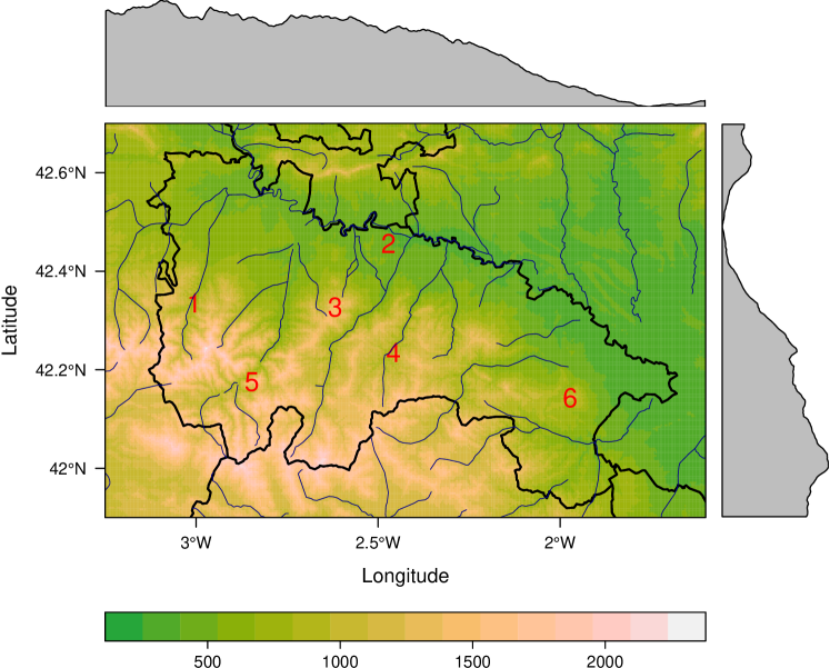
Figure 1: Region analyzed and meteorological stations considered

Table 2: Summary of the meteorological stations selected.

#	Name	Net.	Lat.(º)	Long.(º)	Alt.	$GHI_{a}$
1	Ezcaray	SOS	42.33	-3.00	1000	1479
2	Logroño	SOS	42.45	-2.74	408	1504
3	Moncalvillo	SOS	42.32	-2.61	1495	1329
4	San Roman	SOS	42.23	-2.45	1094	1504
5	Ventrosa	SOS	42.17	-2.84	1565	1277
6	Yerga	SOS	42.14	-1.97	1235	1448

3 Method

This section describes the methodology proposed. Figure 2 displays the method diagram using red ellipses and lines for data sources, blue ellipses and lines for derived rasters (results), and black rectangles and lines for operations.

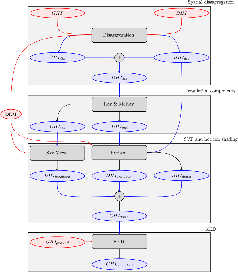
Figure 2: Methodology of downscaling: this figure uses red ellipses and lines for data sources, blue ellipses and lines for derived rasters (results), and black rectangles and lines for operations.

3.1 Irradiation decomposition

Initially, diffuse horizontal irradiation (DHI) is obtained from the difference between global horizontal irradiation (GHI) and beam horizontal irradiation (BHI) rasters, previously obtained from CM SAF. DHI and BHI are firstly disaggregated from the original gross resolution (0.03x0.03^∘) into the DEM resolution (200x200 m), leading to similar values remaining in disaggregated pixels to the original gross resolution pixel. In a second step, DHI can be divided in two components: isotropic diffuse irradiation ($DHI_{iso}$), and anisotropic diffuse irradiation ($DHI_{ani}$) as per the model by Hay & Mckay [Hay and Mckay, 1985] (Equation 1). This model is based on the anisotropy index ($k_{1}$), defined as the ratio of the beam irradiance ($B(0)$) to the extra-terrestrial irradiance ($B_{0}(0)$), as shown in Equation 2. High $k_{1}$ values are typical in clear sky atmospheres, while low $k_{1}$ values are frequent in overcast atmospheres and those with a high aerosol density.

$$DHI=DHI_{iso}+DHI_{ani}$$ (1)

$$k_{1}=\frac{B(0)}{B_{0}(0)}$$ (2)

The $DHI_{iso}$ accounts for the incoming diffuse irradiation portion from an isotropic sky, and is more significant on very cloudy days (Equation 3).

$$DHI_{iso}=DHI\cdot{}(1-k_{1})$$ (3)

$DHI_{ani}$, also denoted as circumsolar diffuse irradiation, considers the incoming portion from the circumsolar disk and can be analyzed as beam irradiation [Perpiñán-Lamigueiro, 2013] (Equation  4).

$$DHI_{ani}=DHI\cdot{}k_{1}$$ (4)

3.2 Sky view factor and horizon blocking

Topographical analysis is performed accounting for the visible sky sphere (sky view) and horizon blocking. The $DHI_{iso}$ is directly dependent on the sky-view factor (SVF), which computes the proportion of visible sky related to a flat horizon. The sky-view factor is considered in earlier irradiation assessments [Ruiz-Arias et al., 2010; Corripio, 2003]. It is calculated in each DEM pixel by considering 72 vectors (separated by 5^∘ each) and evaluating the maximum horizon angle ($\theta_{hor}$) over 20 km in each vector (Equation 5). The $\theta_{hor}$ stands for the maximum angle between the altitude of a location and the elevation of the group of points along each vector, related to a horizontal plane on the location. Locations without horizon blocking have SVFs close to 1, which means a whole visible semi-sphere of sky.

$$SVF=1-\int_{0}^{2\pi}sin^{2}\theta_{hor}d\theta$$ (5)

Eventually, the downscaled $DHI_{iso}$ ($DHI_{iso,down}$) is computed with Equation 6.

$$DHI_{iso,down}=DHI_{iso}\cdot{}SVF$$ (6)

Horizon blocking is analyzed by evaluating the solar geometry in 15 minute samples, particularly the solar elevation ($\gamma_{s}$) and the solar azimuth ($\psi_{s}$). Secondly, the mean hourly $\gamma_{s}$ and $\psi_{s}$ (from those 15 minute rasters) are calculated and then disaggregated as explained above for DHI and BHI rasters. The decision to solve the solar geometry with low resolution rasters enables computation time to be reduced significantly without penalizing the results. The $\theta_{hor}$ corresponding to each $\psi_{s}$ is compared with the $\theta_{zs}$. As a consequence, if the $\theta_{zs}$ is greater than the $\theta_{hor}$, then there is horizon blocking on the surface analyzed and therefore, BHI and $DHI_{ani}$ are blocked. Finally, the sum of $DHI_{ani,down}$, $DHI_{iso,down}$ and $BHI_{iso,down}$ constitutes the downscaled global horizontal irradiation $GHI_{down}$.

3.3 Post-processing: kriging with external drift

The fact that this downscaling accounts for the irradiation loss due to horizon blocking and the sky-view factor leads us to introduce a trend in estimates (lowering them) compared to the original data (gross resolution data). However, satellite-derived irradiation data implicitly considers shade, as a consequence of the lower albedo recorded in these zones, although it is later averaged over the pixel. $GHI_{down}$ can be considered as a useful bias of the behavior of solar irradiation within the region studied. Universal kriging or kriging with external drift (KED) includes information from exhaustively-sampled explanatory variables in the interpolation. As a result, $GHI_{down}$ is considered as the explanatory variable for interpolating measured irradiation data from on-ground calibrated pyranometers, which is denoted as post-processing. $GHI_{down}$ is correlated with the DEM as a consequence of the major influence of horizon blocking with topography, estimations can be derived by separating the deterministic ($\hat{m}(\mathbf{s}_{\theta})$) and stochastic components ($\hat{\epsilon}(\mathbf{s}_{\theta})$ (Equations 7 and  8).

$$\hat{z}(\mathbf{\mathbf{s}}_{\theta})=\hat{m}(\mathbf{s}_{\theta})+\hat{\epsilon}(\mathbf{s}_{\theta})$$ (7)

$$\hat{z}(\mathbf{s}_{\theta})=\sum_{k=0}^{p}\hat{\beta}_{k}q_{k}(\mathbf{s}_{\theta})+\sum_{i=1}^{n}\lambda_{i}\epsilon(\mathbf{s}_{i})$$ (8)

where $\hat{\beta}_{k}$ are the estimated coefficients of the deterministic model, $q_{k}(\mathbf{s}_{\theta})$ are the auxiliary predictors obtained from the fitted values of the explanatory variable at the new location, $\lambda_{i}$ are the kriging weights determined by the spatial dependence structure of the residual, and $\epsilon(\mathbf{s}_{i})$ are the residual at location $\mathbf{s}_{i}$ [Antonanzas-Torres et al., 2013].

The semivariogram is a function defined as Equation 9 based on a constant variance of $\epsilon$ and also on the assumption that spatial correlation of $\epsilon$ depends on the distance amongst instances ($\mathbf{h}$) rather than on their position [Pebesma, 2004].

$$\gamma(\mathbf{h})=\frac{1}{2}\textrm{E}(\epsilon(\mathbf{s})-\epsilon(\mathbf{s}+\mathbf{h}))^{2}$$ (9)

Given that the above sample variogram only collates estimates from observed points, a fitting model of this variogram is generally considered to extrapolate the spatial behavior of observed points to the area studied. In the literature different variogram functions are commonly defined such as the exponential, Gaussian or spherical models. Along these lines, different parameters such as the sill, range and nugget of the model must be adjusted to best fit the sample variogram [Hengl, 2009]. The nugget effect, generally associated with intrinsic micro-variability and measurement error, models the discontinuity of the variogram at the source. It must be highlighted that when the nugget effect is recorded, kriging differs from a regular interpolation and as a result estimates are different from measured values. The variogram model of solar horizontal irradiation is evaluated in Spain, and the conclusion reached is that a pure nugget fitting behaves best, which implies no spatial auto-correlation on residuals [Antonanzas-Torres et al., 2013].

4 Implementation

The method proposed is applied in the region of La Rioja (northern Spain). Figure 3 shows the corresponding annual global horizontal irradiation from CM SAF with resolution 0.03x0.03^∘.

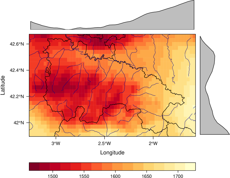
Figure 3: Annual GHI of 2005 from CM SAF estimates (0.03x0.03^∘) in La Rioja

4.1 Packages

The downscaling described in this paper has been implemented using the free software environment R [R Development Core Team, 2013] and various contributed packages:

• raster [Hijmans and van Etten, 2013] for spatial data manipulation and analysis.

• solaR [Perpiñán-Lamigueiro, 2012] for solar geometry.

• gstat [Pebesma and Graeler, 2013] and sp [Pebesma et al., 2013] for geostatistical analysis.

• parallel for multi-core parallelization.

• rasterVis [Perpiñán-Lamigueiro and Hijmans, 2013] for spatial data visualization methods.

⬇

R> library(sp)

R> library(raster)

R> rasterOptions(todisk=FALSE)

R> rasterOptions(chunksize = 1e+06, maxmemory = 1e+07)

R> library(maptools)

R> library(gstat)

R> library(lattice)

R> library(latticeExtra)

R> library(rasterVis)

R> library(solaR)

R> library(parallel)

4.2 Data

Satellite data can be freely downloaded after registration from CM SAF by going to the data access area, selecting web user interface and climate data sets and then choosing the hourly climate data sets named SIS (Global Horizontal Irradiation)) and SID (Beam Horizontal Irradiation) for 2005. Both rasters are projected to the UTM projection for compatibility with the DEM.

⬇

R> projUTM <- CRS(’+proj=utm␣+zone=30’)

R> projLonLat <- CRS(’␣+proj=longlat␣+ellps=WGS84’)

R> listFich <- dir(pattern=’SIShm2005’)

R> stackSIS <- stack(listFich)

R> stackSIS <- projectRaster(stackSIS,crs=projUTM)

R> listFich <- dir(pattern=’SIDhm2005’)

R> stackSID <- stack(listFich)

R> stackSID <- projectRaster(stackSID, crs=projUTM)

We compute the annual global irradiation, which will be used as a reference for subsequent steps.

⬇

R> SISa2005 <- calc(stackSIS, sum, na.rm=TRUE)

The Spanish Digital Elevation Model can be obtained after registration from the ©Spanish Institute of Geography by going to thefree download of digital geographic information for non-commercial use area, and then cropping to the region analyzed (La Rioja). As stated above, this DEM uses the UTM projection.

⬇

R> elevSpain <- raster(’elevSpain.grd’)

R> elev <- crop(elevSpain, extent(479600, 616200, 4639600, 4728400))

R> names(elev)<-’elev’

4.3 Sun geometry

The first step is to compute the sun angles (height and azimuth) and the extraterrestrial solar irradiation for each cell of the CM SAF rasters. The function calcSol from the solaR package calculates the daily and intradaily sun geometry. By means of this function and overlay from the raster package, three multilayer raster objects are generated with the sun geometry needed for the next steps. For the sake of brevity we show only the procedure for extraterrestrial solar irradiation. The sun geometry is calculated with the resolution of CM SAF. First, it is defined a function to extract the hour for aggregation, choose the annual irradiation raster as reference, and define a raster with longitude and latitude coordinates.

⬇

R> hour <- function(tt)as.POSIXct(trunc(tt, ’hours’))

R> r <- SISa2005

R> latlon <- stack(init(r, v=’y’), init(r, v=’x’))

R> names(latlon) <- c(’lat’, ’lon’)

The extraterrestrial irradiation is calculated with 5-min samples. Each point is a column of the data frame locs. Its columns are traversed with lapply, so for each point of the raster object a time series of extraterrestrial solar irradiation is computed. The result, B05min, is a RasterBrick object with a layer for each element of the time index BTi, which is aggregated to an hourly raster with zApply and transformed to the UTM projection.

⬇

R> BTi <- seq(as.POSIXct(’2005-01-01␣00:00:00’),

+ as.POSIXct(’2005-12-31␣23:55:00’), by=’5␣min’)

R> B05min <- overlay(latlon, fun=function(lat, lon){

+ locs <- as.data.frame(rbind(lat, lon))

+ b <- lapply(locs, function(p){

+

+ hh <- local2Solar(BTi, p[2])

+ sol <- calcSol(p[1], BTi=hh)

+ Bo0 <- as.data.frameI(sol)$Bo0

+ Bo0 })

+ res <- do.call(rbind, b)})

R> B05min <- setZ(B05min, BTi)

R> names(B05min) <- as.character(BTi)

R> B0h <- zApply(B05min, by=hour, fun=mean)

R> projectRaster(B0h,crs=projUTM)

4.4 Irradiation components

The CM SAF rasters must be transformed to the higher resolution of the DEM (UTM 200x200 m). Because of the differences in pixel geometry between DEM (square) and irradiation rasters (rectangle) the process is performed in two steps.

The first step increases the spatial resolution of the irradiation rasters to a similar and also larger pixel size than the DEM with disaggregated data, where sf is the scale factor. The second step post-processes the previous step by means of a bilinear interpolation which resamples the raster layer and achieves the same DEM resolution (resample). This two-step disaggregation prevents the loss of the original values of the gross resolution raster that would be directly interpolated with the one-step disaggregation.

⬇

R> sf <- res(stackSID)/res(elev)

R> SIDd <- disaggregate(stackSID, sf)

R> SIDdr <- resample(SIDd, elev)

R> SISd <- disaggregate(stackSIS, sf)

R> SISdr <- resample(SISd, elev)

On the other hand, the diffuse irradiation is obtained from the global and beam irradiation rasters. The two components of the diffuse irradiation, isotropic and anisotropic, can be separated with the anisotropy index, computed as the ratio between beam and extraterrestrial irradiation.

⬇

R> Difdr <- SISdr - SIDdr

R> B0hd <- disaggregate(B0h, sf)

R> B0hdr <- resample(B0hd, elev)

R> k1 <- SIDdr/B0hdr

R> Difiso <- (1-k1) * Difdr

R> Difani <- k1 * Difdr

4.5 Sky view factor and horizon blocking

4.5.1 Horizon angle

The maximum horizon angle required for the horizon blocking analysis and to derive the SVF is obtained with the next code. The alpha vector is visited with mclapply (using parallel computing). For each direction angle (elements of this vector) the maximum horizon angle is calculated for a set of points across that direction from each of the locations defined in xyelev (derived from the DEM raster and transformed in the matrix locs visited by rows).

⬇

R> xyelev <- stack(init(elev, v=’x’),

+ init(elev, v=’y’),

+ elev)

R> names(xyelev) <- c(’x’, ’y’,’elev’)

R> inc <- pi/36

R> alfa <- seq(-0.5*pi,(1.5*pi-inc), inc)

R> locs <- as.matrix(xyelev)

Separations between the source locations and points along each direction are defined by resD, the maximum resolution of the DEM, d, maximum distance to visit, and consequently in the vector seps.

⬇

R> resD <- max(res(elev))

R> d <- 20000

R> seps <- seq(resD, d, by=resD)

The elevation (z1) of each point in xyelev is converted into the horizon angle: the largest of these angles is the horizon angle for that direction. The result of each apply step is a matrix, which is used to fill in a RasterLayer (r). The result of mclapply is a list, hor, of RasterLayer which can be converted into a RasterStack with stack. Each layer of this RasterStack corresponds to a different direction.

⬇

R> hor <- mclapply(alfa, function(ang){

+ h <- apply(locs, 1, function(p){

+ x1 <- p[1]+cos(ang)*seps

+ y1 <- p[2]+sin(ang)*seps

+ p1 <- cbind(x1,y1)

+ z1 <- elevSpain[cellFromXY(elevSpain,p1)]

+ hor <- r2d(atan2(z1-p[3], seps))

+ maxHor <- max(hor[which.max(hor)], 0)

+ })

+ r <- raster(elev)

+ r[] <- matrix(h, nrow=nrow(r), byrow=TRUE)

+ r}, mc.cores=8)

R> horizon <- stack(hor)

This operation is very time-consuming as it is necessary to work with high resolution files. Computation time can be decreased by increasing the sampling space (200 m) or the sectoral angle (5 ^∘) or by reducing the maximum distance (20 km).

4.5.2 Horizon blocking

Horizon blocking is analyzed by evaluating the solar geometry in 15 minute samples, particularly the solar elevation and azimuth angles from the original irradiation raster. Secondly, the hourly averages are calculated, disaggregated and post-processed as explained above for the irradiation rasters. The decision to solve the solar geometry with low resolution rasters enables a significant reduction to be obtained in computation time without penalizing the results.

First, the azimuth raster is cut into different classes according to the alpha vector (directions). The values of the horizon raster corresponding to each angle class are extracted using stackSelect.

⬇

R> idxAngle <- cut(AzShr, breaks=r2d(alfa))

R> AngAlt <- stackSelect(horizon, idxAngle)

The number of layers of AngAlt is the same as idxAngle and can therefore be used for comparison with the solar height angle, AlShr. If AngAlt is greater, there is horizon blocking (dilogical=0).

⬇

R> dilogical <- ((AngAlt-AlShr) < 0)

With this binary raster, beam irradiation and diffuse anisotropic irradiation can be corrected with horizon blocking.

⬇

R> Dirh <- SIDdr * dilogical

R> Difani <- Difani * dilogical

4.5.3 Sky view factor

The sky-view factor can be easily computed from the horizon object with the equation proposed above. This factor corrects the isotropic component of the diffuse irradiation.

⬇

R> SVFRuizArias <- calc(horizon, function(x) sin(d2r(x))^2)

R> SVF <- 1 - mean(SVFRuizArias)

R> Difiso <- Difiso * SVF

Finally, the global irradiation is the sum of the three corrected components, beam and anisotropic diffuse irradiation including horizon blocking, and isotropic diffuse irradiation with the sky view factor.

⬇

R> GHIh <- Difanis + Difiso + Dirh

R> GHI2005a <- calc(GHIh, fun=sum)

4.6 Kriging with external drift

The downscaled irradiation rasters can be improved by using kriging with external drift. Irradiation data from on-ground meteorological stations is interpolated with the downscaled irradiation raster as the explanatory variable. To define the variogram here we use the results previously published in [Antonanzas-Torres et al., 2013].

⬇

R> load(’Stations.RData’)

R> UTM <- SpatialPointsDataFrame(Stations[,c(2,3)], Stations[,-c(2,3)],

+ proj4string=CRS(’+proj=utm␣+zone=30␣+ellps=WGS84’))

R> vgmCMSAF <- variogram(GHImed ~ GHIcmsaf, UTM)

R> fitvgmCMSAF <- fit.variogram(vgmCMSAF, vgm(model=’Nug’))

R> gModel <- gstat(NULL, id=’G0yKrig’,

+ formula= GHImed ~ GHIcmsaf,

+ locations=UTM, model=fitvgmCMSAF)

R> names(GHI2005a) <- ’GHIcmsaf’

R> G0yKrig <- interpolate(GHI2005a, gModel, xyOnly=FALSE)

4.7 Analysis of the results

Figure  3 shows the annual GHI as per CM SAF with the gross resolution analyzed (0.03x0.03^∘) and Figures 4 and  5 show the downscaled maps (200x200 m) without and with the KED.

Figure 4: Annual GHI of 2005 downscaled without KED (0.03x0.03^∘) in La Rioja

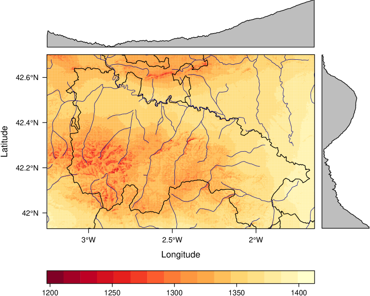
Figure 5: Annual GHI of 2005 downscaled with KED (0.03x0.03^∘) in La Rioja

4.7.1 Model performance

In order to evaluate the performance of the method proposed, relative differences evaluated with station measurements are shown in Figure 6. As can be deduced from this Figure, relative differences are smaller in downscaling with KED than in CM SAF or downscaling without KED, at $\pm$ 15%. The mean absolute error (MAE) and root mean square error (RMSE), described in Equations 10 and 11, are used as indicators of model performance.

$$MAE=\frac{\sum_{i=1}^{n}{\left|{x_{est}-x_{meas}}\right|}}{n}$$ (10)

$$RMSE=\sqrt{\frac{\sum_{i=1}^{n}{(x_{est}-x_{meas})^{2}}}{n}}$$ (11)

where n is number of stations and $x_{est}$ and $x_{meas}$ the annual estimated and measured irradiation, respectively.

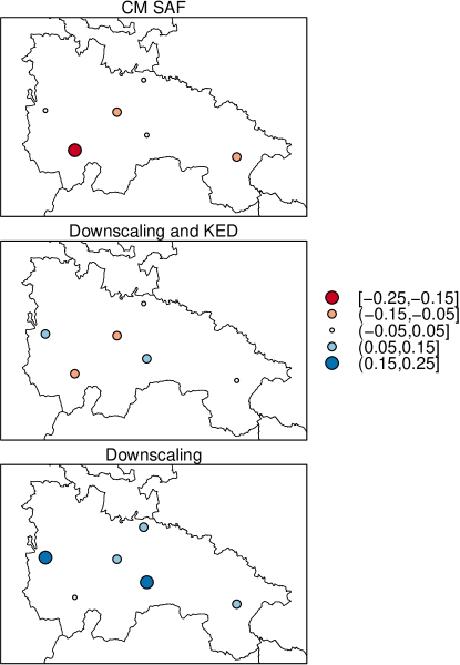
Figure 6: Annual relative differences evaluated with station measurements.

Table  3 shows the MAE and RMSE obtained with CM SAF and with the methodology proposed before and after the KED. The KED leads to a significant improvement in estimates: the MAE is down by 25.5% and the RMSE by 27.4% compared to CM SAF.

	CM SAF	without KED	with KED
MAE	101.35	175.63	75.54
RMSE	118.65	196.53	86.18

Table 3: Summary of errors obtained in $kWh/m^{2}$.

The higher MAE recorded in station locations in CM SAF and downscaling without KED is also explained in the irradiation maps shown in Figures  3 and  4. The $GHI_{annual}$ is lowered too far in certain regions of the area studied with downscaling without KED compared to $GHI_{down,ked}$, which is also shown in Figure 6.

4.7.2 Zonal variability

The intrapixel variability due to the downscaling procedure is indicative of the importance of the topography as an attenuator of solar irrradiation. As a result, this zonal variability is higher in pixels with complex topographies and downscaling is more useful. Figure 7 shows the relative difference between downscaling with KED and CM SAF. As might be deduced, CM SAF over-estimates GHI in this region by between 11 and 22%. Figures  8 and  9 display the standard deviations of the downscaled maps within each cell of the original CM SAF raster (0.03x0.03^∘). The zonal function from the raster library permits this calculation, explaining the intrinsic variability of solar radiation within gross resolution pixels. Consequently, in those pixels with higher standard deviations there will be greater variability . Figure 9 shows how the KED method smooths the deviation within pixels and also the range of solar irradiation in the region (Figures 4 and 5).

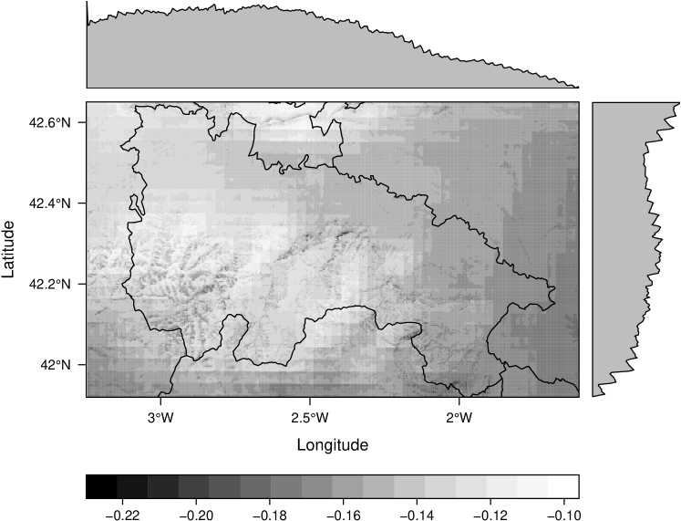
Figure 7: Relative difference of $GHI_{KED}$ and $GHI_{CMSAF,down}$ related to $GHI_{CMSAF,down}$

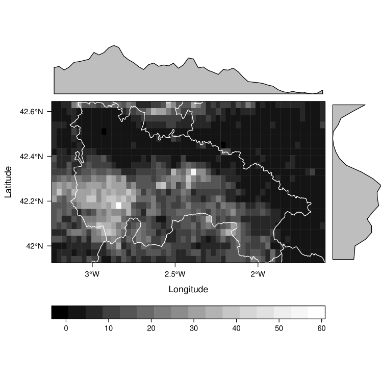
Figure 8: Difference of zonal standard deviations ($kWh/m^{2}$) between downscaling without KED and with KED.

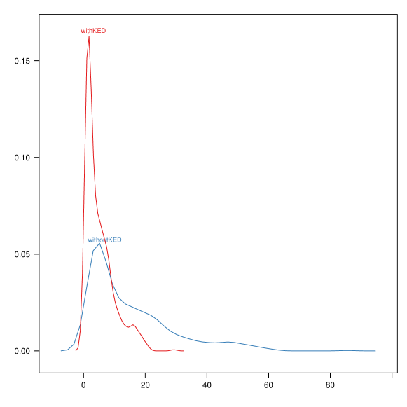
Figure 9: Density plot of zonal standard deviations between CM SAF and downscaling.

5 Concluding comments

A methodology for downscaling solar irradiation is described and presented using R software. This methodology is useful for increasing the accuracy and spatial resolution of gross resolution satellite-estimates of solar irradiation.

It has been proved that areas whose topography is complex show greater differences with the original gross resolution data as a consequence of horizon blocking and lower sky-view factors, so downscaling is highly recommended in these areas.

Kriging with external drift with the gstat package has proved very useful in downscaling solar irradiation when on-ground registers are available and an explanatory variable is provided.

This methodology is implemented as an example in the region of La Rioja in northern Spain, and striking reductions of 25.5% and 27.4% in MAE and RMSE are obtained compared to the original gross resolution database. The high repeatability of this methodology and the reduction in errors obtained might be also very useful in the downscaling of meteorological variables other than solar irradiation.

Software information

The source code is available at https://github.com/EDMANSolar/downscaling. The results discussed in this paper were obtained in a R session with these characteristics:

• R version 2.15.2 (2012-10-26), x86_64-apple-darwin9.8.0

• Locale: es_ES.UTF-8/es_ES.UTF-8/es_ES.UTF-8/C/es_ES.UTF-8/es_ES.UTF-8

• Base packages: base, datasets, graphics, grDevices, grid, methods, parallel, stats,utils

• Other packages: foreign 0.8-51, gstat 1.0-16, hexbin 1.26.0, lattice 0.20-15, latticeExtra 0.6-19, maptools 0.8-14, raster 2.1-16, rasterVis 0.20-01, RColorBrewer 1.0-5, rgdal 0.8-01, solaR 0.33, sp 1.0-8, zoo 1.7-9

• Loaded via a namespace (and not attached): intervals 0.14.0, spacetime 1.0-4, tools 2.15.2, xts 0.9-3

References

- Alsamamra et al. [2009] Husain Alsamamra, Jose Antonio Ruiz-Arias, David Pozo-Vázquez, and Joaquin Tovar-Pescador. A comparative study of ordinary and residual kriging techniques for mapping global solar radiation over southern spain. Agricultural and Forest Meteorology, 149(8):1343 – 1357, 2009.
- Antonanzas-Torres et al. [2013] Fernando Antonanzas-Torres, Federico Cañizares, and Oscar Perpiñán. Comparative assessment of global irradiation from a satellite estimate model (CM SAF) and on-ground measurements (SIAR): a spanish case study. Renewable and Sustainable Energy Reviews, 21:248–261, 2013.
- Batlles et al. [2008] F.J. Batlles, J.L. Bosch, J. Tovar-Pescador, M. Martínez-Durbán, R. Ortega, and I. Miralles. Determination of atmospheric parameters to estimate global radiation in areas of complex topography: Generation of global irradiation map. Energy Conversion and Management, 49(2):336 – 345, 2008.
- Bosch et al. [2010] J.L. Bosch, F.J. Batlles, L.F. Zarzalejo, and G. López. Solar resources estimation combining digital terrain models and satellite images techniques. Renewable Energy, 35(12):2853 – 2861, 2010.
- Corripio [2003] J. Corripio. Vectorial algebra algorithms for calculating terrain parameters from dems and solar radiation modelling in mountainous terrain. International Journal of Geographical Information Science, 17:1–23, 2003.
- Hay and Mckay [1985] E. Hay and D.C. Mckay. Estimating solar irradiance on inclined surfaces: a review and assessment of methodologies. International Journal of Solar Energy, 3:203–240, 1985.
- Hengl [2009] T. Hengl. A Practical Guide to Geostatistical Mapping. 2009. URL http://spatial-analyst.net/book/.
- Hijmans and van Etten [2013] Robert J. Hijmans and Jacob van Etten. raster: Geographic Data Analysis and Modeling, 2013. URL http://CRAN.R-project.org/package=raster. R package version 2.1-25.
- Pebesma [2004] E. J. Pebesma. Multivariable geostatistics in S: the gstat package. Computers & Geosciences, 30:683–691, 2004.
- Pebesma and Graeler [2013] Edzer Pebesma and Benedikt Graeler. gstat: Spatial and Spatio-Temporal Geostatistical Modelling, Prediction and Simulation, 2013. URL http://CRAN.R-project.org/package=gstat. R package version 1.0-16.
- Pebesma et al. [2013] Edzer Pebesma, Roger Bivand, Barry Rowlingson, and Virgilio Gomez-Rubio. sp: Classes and Methods for Spatial Data, 2013. URL http://CRAN.R-project.org/package=sp. R package version 1.0-9.
- Perez et al. [1994] Richard Perez, Robert Seals, Ronald Stewart, Antoine Zelenka, and Vicente Estrada-Cajigal. Using satellite-derived insolation data for the site/time specific simulation of solar energy systems. Solar Energy, 53(6):491 – 495, 1994.
- Perpiñán-Lamigueiro [2012] Oscar Perpiñán-Lamigueiro. solaR: Solar radiation and photovoltaic systems with R. Journal of Statistical Software, 50(9):1–32, 8 2012. ISSN 1548-7660. URL http://www.jstatsoft.org/v50/i09.
- Perpiñán-Lamigueiro [2013] Oscar Perpiñán-Lamigueiro. Energía Solar Fotovoltaica. 2013. URL http://procomun.wordpress.com/documentos/libroesf/.
- Perpiñán-Lamigueiro and Hijmans [2013] Oscar Perpiñán-Lamigueiro and Robert J. Hijmans. rasterVis: Visualization Methods for the Raster Package, 2013. URL http://CRAN.R-project.org/package=rasterVis. R package version 0.20-07.
- Posselt et al. [2011] R. Posselt, R. Muller, J. Trentmann, and R. Stockli. Meteosat (mviri) solar surface irradiance and effective cloud albedo climate data sets. the cm saf validation report. Technical report, The EUMETSAT Network of Satellite Application Facilities, 2011.
- Posselt et al. [2012] R. Posselt, R.W. Mueller, R. Stöckli, and J. Trentmann. Remote sensing of solar surface radiation for climate monitoring — the cm-saf retrieval in international comparison. Remote Sensing of Environment, 118(0):186 – 198, 2012.
- R Development Core Team [2013] R Development Core Team. R: A Language and Environment for Statistical Computing. R Foundation for Statistical Computing, Vienna, Austria, 2013. URL http://www.R-project.org. ISBN 3-900051-07-0.
- Ruiz-Arias et al. [2010] José A. Ruiz-Arias, Tomáš Cebecauer, Joaquín Tovar-Pescador, and Marcel Šúri. Spatial disaggregation of satellite-derived irradiance using a high-resolution digital elevation model. Solar Energy, 84(9):1644 – 1657, 2010.
- Schulz et al. [2009] J. Schulz, P. Albert, H.-D. Behr, D. Caprion, H. Deneke, S. Dewitte, B. Dürr, P. Fuchs, A. Gratzki, P. Hechler, R. Hollmann, S. Johnston, K.-G. Karlsson, T. Manninen, R. Müller, M. Reuter, A. Riihelä, R. Roebeling, N. Selbach, A. Tetzlaff, W. Thomas, M. Werscheck, E. Wolters, and A. Zelenka. Operational climate monitoring from space: the eumetsat satellite application facility on climate monitoring (cm-saf). Atmospheric Chemistry and Physics, 9(5):1687–1709, 2009.