On critical behaviour in systems of Hamiltonian partial differential equations

B. Dubrovin, T. Grava, C. Klein, A. Moro
Abstract

We study the critical behaviour of solutions to weakly dispersive Hamiltonian systems considered as perturbations of elliptic and hyperbolic systems of hydrodynamic type with two components. We argue that near the critical point of gradient catastrophe of the dispersionless system, the solutions to a suitable initial value problem for the perturbed equations are approximately described by particular solutions to the Painlevé-I (PI) equation or its fourth order analogue P2Isuperscriptsubscriptabsent𝐼2{}_{I}^{2}. As concrete examples we discuss nonlinear Schrödinger equations in the semiclassical limit. A numerical study of these cases provides strong evidence in support of the conjecture.

1 Introduction

Critical phenomena in the solutions of partial differential equations (PDEs) are important from various theoretical and applied points of view since such phenomena generally indicate the appearence of new behaviours as the onset of rapid oscillations, the appearence of multiple scales, or a loss of regularity in the solutions. Some of the most powerful techniques in the asymptotic description of such phenomena are due to the theory of completely integrable systems which were so far restricted to integrable PDEs. In [43] this restriction was overcome by introducing the concept of integrability up to a finite order of some small parameter ϵitalic-ϵ\epsilon. This has allowed to apply techniques from the theory of integrable systems to a large class of non-integrable equations and to obtain asymptotic descriptions of solutions to such equations in the vicinity of critical points of these PDEs. The scalar case was studied along these lines in [43]. Basically it was shown that solutions to dispersive regularizations of a nonlinear transport equation near a point of gradient catastrophe (for the transport equation itself) behave like solutions of the celebrated Korteweg–de Vries equations, which at such point can be asymptotically expressed in terms of a particular solution to a fourth order ordinary differential equation from the Painlevé-I family. In [46] this concept was generalized to the study of the semiclassical limit of the integrable focusing cubic nonlinear Schrödinger equation (NLS) which can be seen as a perturbation of 2×2222\times 2 elliptic system and in [44] to a certain class of integrable Hamiltonian perturbation of 2×2222\times 2 elliptic and hyperbolic systems. The idea that integrable behaviour persists in certain nonintegrable cases has been already developed in the study of long time behaviour of solutions to several nonintegrable equations, like the pertuberd NLS equation [39], see also [114] for a general overview about the soliton resolution conjecture.

In this paper we consider general two-component Hamiltonian systems which contain a small dispersion parameter ϵitalic-ϵ\epsilon. When ϵ=0italic-ϵ0\epsilon=0 the Hamiltonian system reduces to a 2×2222\times 2 quasilinear system of elliptic or hyperbolic type, so that the Hamiltonian system can be considered as a perturbation of the elliptic or hyperbolic systems. We study the behaviour of solutions to such Hamiltonian systems when the parameter ϵitalic-ϵ\epsilon tends to zero. The fundamental question we address is how does a solution to Hamiltonian equations behave near the point where the solution of the unperturbed elliptic or hyperbolic system breaks up.

We consider Hamiltonian PDEs obtained as perturbations of systems of hydrodynamic type of the form

ut=xδH0δv(x)xhvsubscript𝑢𝑡subscript𝑥𝛿subscript𝐻0𝛿𝑣𝑥subscript𝑥𝑣\displaystyle u_{t}=\partial_{x}\frac{\delta H_{0}}{\delta v(x)}\equiv\partial_{x}\frac{\partial h}{\partial v}
(1.1)
vt=xδH0δu(x)xhu,subscript𝑣𝑡subscript𝑥𝛿subscript𝐻0𝛿𝑢𝑥subscript𝑥𝑢\displaystyle v_{t}=\partial_{x}\frac{\delta H_{0}}{\delta u(x)}\equiv\partial_{x}\frac{\partial h}{\partial u},

with u=u(x,t)𝑢𝑢𝑥𝑡u=u(x,t), v=v(x,t)𝑣𝑣𝑥𝑡v=v(x,t), scalar functions, x𝑥x\in\mathbb{R} and

H0=h(u,v)𝑑x,subscript𝐻0𝑢𝑣differential-d𝑥H_{0}=\int h(u,v)\,dx,

where h=h(u,v)𝑢𝑣h=h(u,v) is a smooth function of u𝑢u and v𝑣v. Such perturbations can be written in the form

ut=xδHδv(x)subscript𝑢𝑡subscript𝑥𝛿𝐻𝛿𝑣𝑥\displaystyle u_{t}=\partial_{x}\frac{\delta H}{\delta v(x)}
(1.2)
vt=xδHδu(x).subscript𝑣𝑡subscript𝑥𝛿𝐻𝛿𝑢𝑥\displaystyle v_{t}=\partial_{x}\frac{\delta H}{\delta u(x)}.

where H𝐻H is the perturbed Hamiltonian, H=H0+ϵH1+ϵ2H2+𝐻subscript𝐻0italic-ϵsubscript𝐻1superscriptitalic-ϵ2subscript𝐻2H=H_{0}+\epsilon\,H_{1}+\epsilon^{2}H_{2}+\dots. By definition the k𝑘k-th order term of the perturbative expansion must have the form

Hk=hk(u,v,ux,vx,uxx,vxx,,u(k),v(k))𝑑xsubscript𝐻𝑘subscript𝑘𝑢𝑣subscript𝑢𝑥subscript𝑣𝑥subscript𝑢𝑥𝑥subscript𝑣𝑥𝑥superscript𝑢𝑘superscript𝑣𝑘differential-d𝑥H_{k}=\int h_{k}\left(u,v,u_{x},v_{x},u_{xx},v_{xx},\dots,u^{(k)},v^{(k)}\right)\,dx

where hk(u,v,ux,vx,uxx,vxx,,u(k),v(k))subscript𝑘𝑢𝑣subscript𝑢𝑥subscript𝑣𝑥subscript𝑢𝑥𝑥subscript𝑣𝑥𝑥superscript𝑢𝑘superscript𝑣𝑘h_{k}\left(u,v,u_{x},v_{x},u_{xx},v_{xx},\dots,u^{(k)},v^{(k)}\right) is a graded homogeneous polynomial of degree k𝑘k in the variables uxsubscript𝑢𝑥u_{x}, vxsubscript𝑣𝑥v_{x}, …, u(k)superscript𝑢𝑘u^{(k)}, v(k)superscript𝑣𝑘v^{(k)}, i.e., it satisfies the identity

hk(u,v,λux,λvx,λ2uxx,λ2vxx,,λku(k),λkv(k))=λkhk(u,v,ux,vx,uxx,vxx,,u(k),v(k))subscript𝑘𝑢𝑣𝜆subscript𝑢𝑥𝜆subscript𝑣𝑥superscript𝜆2subscript𝑢𝑥𝑥superscript𝜆2subscript𝑣𝑥𝑥superscript𝜆𝑘superscript𝑢𝑘superscript𝜆𝑘superscript𝑣𝑘superscript𝜆𝑘subscript𝑘𝑢𝑣subscript𝑢𝑥subscript𝑣𝑥subscript𝑢𝑥𝑥subscript𝑣𝑥𝑥superscript𝑢𝑘superscript𝑣𝑘h_{k}\left(u,v,\lambda\,u_{x},\lambda\,v_{x},\lambda^{2}u_{xx},\lambda^{2}v_{xx},\dots,\lambda^{k}u^{(k)},\lambda^{k}v^{(k)}\right)=\lambda^{k}h_{k}\left(u,v,u_{x},v_{x},u_{xx},v_{xx},\dots,u^{(k)},v^{(k)}\right)

for an arbitrary λ𝜆\lambda. The Hamiltonian system (1) can be considered as a weakly dispersive perturbation of the 1st order quasilinear system (1).

After certain simplification of the system (1) by a suitable class of ϵitalic-ϵ\epsilon-dependent canonical transformations

u(x)u~(x)=u(x)+ϵ{u(x),F}+𝒪(ϵ2)maps-to𝑢𝑥~𝑢𝑥𝑢𝑥italic-ϵ𝑢𝑥𝐹𝒪superscriptitalic-ϵ2\displaystyle u(x)\mapsto\tilde{u}(x)=u(x)+\epsilon\,\{u(x),F\}+{\mathcal{O}}(\epsilon^{2})
v(x)v~(x)=v(x)+ϵ{v(x),F}+𝒪(ϵ2)maps-to𝑣𝑥~𝑣𝑥𝑣𝑥italic-ϵ𝑣𝑥𝐹𝒪superscriptitalic-ϵ2\displaystyle v(x)\mapsto\tilde{v}(x)=v(x)+\epsilon\,\{v(x),F\}+{\mathcal{O}}(\epsilon^{2})

generated by a Hamiltonian F𝐹F (see Section 2) the system can be spelled out as follows

ut=xδHδv(x)=huvux+hvvvxsubscript𝑢𝑡subscript𝑥𝛿𝐻𝛿𝑣𝑥subscript𝑢𝑣subscript𝑢𝑥subscript𝑣𝑣subscript𝑣𝑥\displaystyle u_{t}=\partial_{x}\frac{\delta H}{\delta v(x)}=h_{uv}u_{x}+h_{vv}v_{x}
+ϵ2[buxxx+cvxxx+(av+3bu)uxxux+(bv+cu)uxxvx+2cuvxxux+2cvvxxvx\displaystyle+\epsilon^{2}\left[b\,u_{xxx}+c\,v_{xxx}+(-a_{v}+3b_{u})u_{xx}u_{x}+(b_{v}+c_{u})u_{xx}v_{x}+2c_{u}v_{xx}u_{x}+2c_{v}v_{xx}v_{x}\right.
+(12auv+buu)ux3+(12avv+buv+cuu)ux2vx+32cuvuxvx2+12cvvvx3]\displaystyle\left.+\left(-\frac{1}{2}a_{uv}+b_{uu}\right)u_{x}^{3}+\left(-\frac{1}{2}a_{vv}+b_{uv}+c_{uu}\right)u_{x}^{2}v_{x}+\frac{3}{2}c_{uv}u_{x}v_{x}^{2}+\frac{1}{2}c_{vv}v_{x}^{3}\right]
(1.3)
vt=xδHδu(x)=huuux+huvvxsubscript𝑣𝑡subscript𝑥𝛿𝐻𝛿𝑢𝑥subscript𝑢𝑢subscript𝑢𝑥subscript𝑢𝑣subscript𝑣𝑥\displaystyle v_{t}=\partial_{x}\frac{\delta H}{\delta u(x)}=h_{uu}u_{x}+h_{uv}v_{x}
+ϵ2[auxxx+bvxxx+2auuxxux+2avuxxvx+(av+bu)vxxux+(3bvcu)vxxvx\displaystyle+\epsilon^{2}\left[a\,u_{xxx}+b\,v_{xxx}+2a_{u}u_{xx}u_{x}+2a_{v}u_{xx}v_{x}+(a_{v}+b_{u})v_{xx}u_{x}+(3b_{v}-c_{u})v_{xx}v_{x}\right.
+12auuux3+32auvux2vx+(avv+buv12cuu)uxvx2+(bvv12cuv)vx3]\displaystyle\left.+\frac{1}{2}a_{uu}u_{x}^{3}+\frac{3}{2}a_{uv}u_{x}^{2}v_{x}+\left(a_{vv}+b_{uv}-\frac{1}{2}c_{uu}\right)u_{x}v_{x}^{2}+\left(b_{vv}-\frac{1}{2}c_{uv}\right)v_{x}^{3}\right]

up to terms of order ϵ3superscriptitalic-ϵ3\epsilon^{3}. Here a=a(u,v)𝑎𝑎𝑢𝑣a=a(u,v), b=b(u,v)𝑏𝑏𝑢𝑣b=b(u,v) and c=c(u,v)𝑐𝑐𝑢𝑣c=c(u,v) are arbitrary smooth functions of u𝑢u and v𝑣v at least in the domain where the solution of the unperturbed equation (1) takes values. The corresponding perturbed Hamiltonian reads

H=H0+ϵ2H2=[hϵ22(aux2+2buxvx+cvx2)]𝑑x𝐻subscript𝐻0superscriptitalic-ϵ2subscript𝐻2delimited-[]superscriptitalic-ϵ22𝑎superscriptsubscript𝑢𝑥22𝑏subscript𝑢𝑥subscript𝑣𝑥𝑐superscriptsubscript𝑣𝑥2differential-d𝑥H=H_{0}+\epsilon^{2}H_{2}=\int\left[h-\frac{\epsilon^{2}}{2}\left(a\,u_{x}^{2}+2b\,u_{x}v_{x}+c\,v_{x}^{2}\right)\right]\,dx (1.4)

The family of equations of the form (1) contains important examples such as the generalised nonlinear Schrödinger (NLS) equations (also in a nonlocal version), the long wave limit of lattice equations like the Fermi–Pasta–Ulam or Toda lattice equation, Boussinesq equation, two-component Camassa–Holm equation [52] and many others. For certain choices of the functions h(u,v)𝑢𝑣h(u,v), a(u,v)𝑎𝑢𝑣a(u,v), b(u,v)𝑏𝑢𝑣b(u,v) and c(u,v)𝑐𝑢𝑣c(u,v), the system of equations (1) is integrable up to the order ϵ3superscriptitalic-ϵ3\epsilon^{3} [44]. However the complete classification of integrable cases in the class of equations of the form (1) remains open, see [40], [48], [84] for the current state of the art in this context.

The study of scalar weakly dispersive equations

ut=xδHδu(x)=x(h(u)+ϵ2[a(u)uxx+12a(u)ux2]+𝒪(ϵ3))subscript𝑢𝑡subscript𝑥𝛿𝐻𝛿𝑢𝑥subscript𝑥superscript𝑢superscriptitalic-ϵ2delimited-[]𝑎𝑢subscript𝑢𝑥𝑥12superscript𝑎𝑢superscriptsubscript𝑢𝑥2𝒪superscriptitalic-ϵ3\displaystyle u_{t}=\partial_{x}\frac{\delta H}{\delta u(x)}=\partial_{x}\left(h^{\prime}(u)+\epsilon^{2}\left[a(u)u_{xx}+\frac{1}{2}a^{\prime}(u)u_{x}^{2}\right]+{\mathcal{O}}\left(\epsilon^{3}\right)\right)
H=[h(u)ϵ22a(u)ux2+]𝑑x𝐻delimited-[]𝑢superscriptitalic-ϵ22𝑎𝑢superscriptsubscript𝑢𝑥2differential-d𝑥\displaystyle H=\int\left[h(u)-\frac{\epsilon^{2}}{2}a(u)u_{x}^{2}+\dots\right]\,dx

of the form similar to (1), (1.4) in the limit ϵ0italic-ϵ0\epsilon\rightarrow 0 in the strongly nonlinear regime was initiated by the seminal paper by Gurevich and Pitaevsky [65] about “collisionless shock waves” described by KdV equation (see also the book [104] and references therein). Rigorous mathematical results in this direction were obtained by Lax, Levermore and Venakides [88], [89], [124] and Deift, Venakides and Zhou [38] (see also [62] and [60] for numerical comparison). For two-component systems (1) an analogous line of research was started with the works [22], [55], [63] on the semiclassical limit of generalized defocusing nonlinear Schrödinger equation in several space dimensions for times less than the critical time t0subscript𝑡0t_{0} of the cusp catastrophe. It was studied in more details for arbitrary times for the integrable case [128], namely for the spatially one-dimensional cubic defocusing NLS in [71], [72], [41]. Another system that is included in the class (1) is the long wave limit of the Toda lattice equation that has been studied in detail for arbitrary times in [37] and, in the context of Hermitian random matrix models with exponential weights by many authors, see the book [34] and references therein. Interesting results, in the spirit of the original Gurevich and Pitaevsky setting, have been obtained for certain nonintegrable cases in [51], [67]. Possible relations between integrable and non-integrable behaviour have been also analyzed in the framework of the long wave limit of the Fermi–Pasta–Ulam system by Zabusky and Kruskal [128] and, more recently, in [5], [92], [8].

The study of solutions to Hamiltonian systems of the form (1) in the limit ϵ0italic-ϵ0\epsilon\rightarrow 0 whith the leading term (1) of elliptic type was initiated by the analysis of the semiclassical limit of the focusing cubic nonlinear Schrödinger equation [75], see also [19], [24] [94], [119], [120]. Other interesting Hamiltonian systems not included in the class (1) have been considered in the limit ϵ0italic-ϵ0\epsilon\rightarrow 0 in [98], [20].

Our study can be considered as a continuation of the programme initiated in [43], [44] and [46] aimed at studying critical behaviour of Hamiltonian perturbations of quasilinear hyperbolic and elliptic PDEs. The most important of the concepts developped in these papers is the idea of universality of the critical behaviour. We borrow this notion from the theory of random matrices where various universality types of critical behaviour appear in the study of phase transitions in random matrix ensembles, see for example [14], [12], [35], [36], [50], [26] for mathematically oriented references. The description of the critical behaviour for generalized Burgers equation with small viscosity was found by Il’in [69]; for more general weakly dissipative equations see [45], [4].

In the present paper solutions u(x,t;ϵ)𝑢𝑥𝑡italic-ϵu(x,t;\epsilon), v(x,t;ϵ)𝑣𝑥𝑡italic-ϵv(x,t;\epsilon) to the Cauchy problem

u(x,0;ϵ)=u0(x),v(x,0;ϵ)=v0(x)formulae-sequence𝑢𝑥0italic-ϵsubscript𝑢0𝑥𝑣𝑥0italic-ϵsubscript𝑣0𝑥u(x,0;\epsilon)=u_{0}(x),\quad v(x,0;\epsilon)=v_{0}(x) (1.5)

for the system (1) with ϵitalic-ϵ\epsilon-independent smooth initial data in a suitable functional class will be under consideration. The contribution of higher order terms is believed to be negligible as long as the solution (u(x,t;ϵ),v(x,t;ϵ))𝑢𝑥𝑡italic-ϵ𝑣𝑥𝑡italic-ϵ\left(u(x,t;\epsilon),v(x,t;\epsilon)\right) remains a slowly varying function of x𝑥x and t𝑡t, that is, it changes by 𝒪(1)𝒪1{\cal O}(1) on the space- and time-scale of order 𝒪(ϵ1)𝒪superscriptitalic-ϵ1{\cal O}\left(\epsilon^{-1}\right). A rigorous proof of such a statement would justify existence, for sufficiently small values of the parameter ϵitalic-ϵ\epsilon, of the solution to the Cauchy problem (1), (1.5) on a finite time interval 0tt00𝑡subscript𝑡00\leq t\leq t_{0} depending on the initial condition but not on ϵitalic-ϵ\epsilon. This was proven by Lax, Levermore and Venakides [88], [89] for the particular case of the Korteweg - de Vries (KdV) equation with rapidly decreasing initial data. In a more general setting of a certain class of generalized KdV equations with no integrability assumption, the statement was proven more recently in [97].

Actually we expect validity of a more bold statement that, in particular, gives an efficient upper bound for the life span of a solution to (1) with given initial data (1.5). Namely, we start with considering the solution (u(x,t),v(x,t))𝑢𝑥𝑡𝑣𝑥𝑡\left(u(x,t),v(x,t)\right) to the Cauchy problem for the unperturbed system (1) with the same initial data111Analyticity of the initial data will be assumed in case the quasilinear system (1) is of elliptic type. The precise formulation of our Main Conjecture has to be refined in the non analytic case

u(x,0)=u0(x),v(x,0)=v0(x).formulae-sequence𝑢𝑥0subscript𝑢0𝑥𝑣𝑥0subscript𝑣0𝑥u(x,0)=u_{0}(x),\quad v(x,0)=v_{0}(x).

Such a solution exists for times below the time t0subscript𝑡0t_{0} of gradient catastrophe. We expect that the life span of the perturbed solution (u(x,t;ϵ),v(x,t;ϵ))𝑢𝑥𝑡italic-ϵ𝑣𝑥𝑡italic-ϵ\left(u(x,t;\epsilon),v(x,t;\epsilon)\right) for sufficiently small ϵitalic-ϵ\epsilon is at least the interval [0,t0]0subscript𝑡0[0,t_{0}]. More precisely, we have the following

Main Conjecture.

Part 1. There exists a positive constant Δt(ϵ)>0Δ𝑡italic-ϵ0\Delta t(\epsilon)>0 depending on the initial condition (1.5) such that the solution to the Cauchy problem (1), (1.5) exists for 0t<t0+Δt(ϵ)0𝑡subscript𝑡0Δ𝑡italic-ϵ0\leq t<t_{0}+\Delta t(\epsilon) for sufficiently small ϵitalic-ϵ\epsilon.

Part 2. When ϵ0italic-ϵ0\epsilon\to 0 the perturbed solution (u(x,t;ϵ),v(x,t;ϵ))𝑢𝑥𝑡italic-ϵ𝑣𝑥𝑡italic-ϵ\left(u(x,t;\epsilon),v(x,t;\epsilon)\right) converges to the unperturbed one (u(x,t),v(x,t))𝑢𝑥𝑡𝑣𝑥𝑡\left(u(x,t),v(x,t)\right) uniformly on compacts x1xx2subscript𝑥1𝑥subscript𝑥2x_{1}\leq x\leq x_{2}, 0tt10𝑡subscript𝑡10\leq t\leq t_{1} for any t1<t0subscript𝑡1subscript𝑡0t_{1}<t_{0} and arbitrary x1subscript𝑥1x_{1} and x2subscript𝑥2x_{2}.

In the Main Conjecture we do not specify the class of boundary conditions for the smooth (or even analytic, in the elliptic case) initial data u0(x)subscript𝑢0𝑥u_{0}(x), v0(x)subscript𝑣0𝑥v_{0}(x). We believe that the statement is applicable to a wide class of boundary conditions like rapidly decreasing, step-like, periodic etc. Moreover, the shape of the universal critical behavior at the point of catastrophe (see below) should be independent of the choice of boundary conditions.

The last statement of the Main Conjecture refers to the behavior of a generic perturbed solution near the point of gradient catastrophe of the unperturbed one. Our main goal is to find an asymptotic description for the dispersive regularisation of the elliptic umbilic singularity or the cusp catastrophe when the dispersive terms are added, i.e., we want to describe the leading term of the asymptotic behaviour for ϵ0italic-ϵ0\epsilon\to 0 of the solution to (1) near the critical point, say (x0,t0)subscript𝑥0subscript𝑡0(x_{0},t_{0}), of a generic solution to (1).

At the point of catastrophe the solutions u(x,t)𝑢𝑥𝑡u(x,t), v(x,t)𝑣𝑥𝑡v(x,t) to the Cauchy problem (1), (1.5) remain continuous, but their derivatives blow up. The generic singularities are classified as follows [43], [44].

  • If the system (1) is elliptic, huuhvv<0subscript𝑢𝑢subscript𝑣𝑣0h_{uu}h_{vv}<0, then the generic singularity is a point of elliptic umbilic catastrophe. This codimension 2 singularity is one of the real forms labeled by the root system of the D4subscript𝐷4D_{4} type in the terminology of Arnold et al. [3].

  • If the system (1) is hyperbolic, huuhvv>0subscript𝑢𝑢subscript𝑣𝑣0h_{uu}h_{vv}>0, then the generic singularity is a point of cusp catastrophe or more precisely the Whitney W3 [4] singularity.

Elliptic umbilic singularities appear in experimental and theoretical studies of diffraction in more than one spatial dimension [11], in plasma physics [111], [110], in the Hele–Shaw problem [96], and also in random matrices, [53], [12]. Formation of singularities for general quasi-linear hyperbolic systems in many spatial dimensions has been considered in [2] (see [95] for an explicit example). For the particular case of 2×2222\times 2 systems we are mainly dealing with, the derivation of the cusp catastrophe was obtained for 𝒞4superscript𝒞4\mathcal{C}^{4} initial data in [85], see also [44] for an alternative derivation.

Let us return to the Cauchy problem for the perturbed system (1) with the same initial data (1.5). The fundamental idea of universality first formulated in [43] for scalar Hamiltonian PDEs suggests that, at the leading order of asymptotic approximation, such behavior does depend neither on the choice of generic initial data nor on the choice of generic Hamiltonian perturbation. One of the goals of the present paper is to give a precise formulation of the universality conjecture for a quite general class of systems of Hamiltonian PDEs of order two (for certain particular subclasses of such PDEs the universality conjecture has already been formulated in [44]).

The general formulation of universality introduced in [43] for the case of Hamiltonian perturbations of the scalar nonlinear transport equation and in [44] for Hamiltonian perturbation of the nonlinear wave equation says that the leading term of the multiscale asymptotics of the generic solution near the critical point does not depend on the choice of the solution, modulo Galilean transformations and rescalings. This leading term was identified via a particular solution to the fourth order analogue of the Painlevé-I (PI) equation (the so-called P2Isuperscriptsubscriptabsent𝐼2{}_{I}^{2} equation). Earlier the particular solution to the P2Isuperscriptsubscriptabsent𝐼2{}_{I}^{2} equation proved to be important in the theory of random matrices [102], [18]; in the context of the so-called Gurevich–Pitaevsky solution to the KdV equation it was derived in [79]. The existence of the needed smooth solution to P2Isuperscriptsubscriptabsent𝐼2{}_{I}^{2} has been rigorously established in [27]. Moreover, it was argued in [43] and [44] that the shape of the leading term describing the critical behaviour is essentially independent on the particular form of the Hamiltonian perturbation. Some of these universality conjectures have been supported by numerical experiments carried out in [63], [47]. The rigourous analytical proof of this conjecture has been obtained for the KdV equation in [25].

In [46] the universality conjecture for the critical behaviour of solutions to the focusing cubic NLS has been formulated, and in [44] the universality conjecture has been extended to other integrable Hamiltonian perturbations of elliptic systems. The universality conjecture in this case suggests that the description of the leading term in the asymptotic expansion of the solution to the focusing NLS equation in the semiclassical limit, near the point of elliptic umbilic catastrophe, is given via a particular solution to the classical Painlevé-I equation (PI), namely the tritronquée solution first introduced by Boutroux [16] one hundred years ago; see [73], [77] regarding some important properties of the tritronquée solution and its characterization in the framework of the theory of isomonodromy deformations. The smoothness of the tritronquée solution in a sector of the complex z𝑧z-plane of angle |argz|<4π/5𝑧4𝜋5|\arg z|<4\pi/5 conjectured in [46] has only recently been proved in [30]. Other arguments supporting the universality conjecture for the focusing case were found in [13].

In this paper we extend these ideas to the more general class of systems of the form (1). More precisely, our main goal is a precise formulation of the following conjectural statement.

Main Conjecture, Part 3.

  • The solution of the generic system (1) with generic ϵitalic-ϵ\epsilon-independent analytic initial data near a point of elliptic umbilic catastrophe of the unperturbed elliptic system (1) in the limit ϵ0italic-ϵ0\epsilon\rightarrow 0 is described by the tritronquée solution to the PI equation;

  • the solution of the generic system (1) with generic ϵitalic-ϵ\epsilon-independent smooth initial data near a point of cusp catastrophe of the unperturbed hyperbolic system (1) is described in the limit ϵ0italic-ϵ0\epsilon\rightarrow 0 by a particular solution to the P2Isuperscriptsubscriptabsent𝐼2{}_{I}^{2} equation.

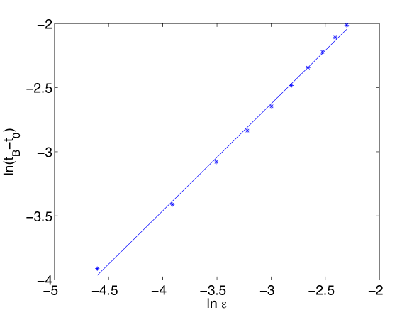
An important aspect of the above conjectures is the existence of the solution of the perturbed Hamiltonian systems (1) for times t𝑡t up to and slightly beyond the critical time t0subscript𝑡0t_{0} for the solution of the unperturbed system (1). The study of the local or global well-posedness of the Cauchy problem for the full class of equations (1) remains open even though a large class of equations has been studied, see for example [58] or [115], [93], [15] for a survey of the state-of-the-art. For finite ϵitalic-ϵ\epsilon it is known that the solution of the Cauchy problem of certain classes of equations of the form (1) develops blow-up in finite time, see for example [113], [81]. For the class of equations of the form (1) and initial data such that the solution develops a blow up in finite time tBsubscript𝑡𝐵t_{B}, we consequentially conjecture that, for sufficiently small ϵitalic-ϵ\epsilon, the blow-up time tBsubscript𝑡𝐵t_{B} is always larger than the critical time t0subscript𝑡0t_{0} of the dispersionless system. The blow-up behaviour of solutions to certain class of equations, like the focusing NLS equation has been studied in detail in [99], however the issue of the determination of the blow-up time remains open. For the particular case of the quintic focusing NLS equation, we claim that the blow-up time tBsubscript𝑡𝐵t_{B} which depends on ϵitalic-ϵ\epsilon is close in the limit ϵ0italic-ϵ0\epsilon\rightarrow 0 to the time of elliptic umbilic catastrophe, more precisely the ratio (tBt0)/ϵ45subscript𝑡𝐵subscript𝑡0superscriptitalic-ϵ45(t_{B}-t_{0})/\epsilon^{\frac{4}{5}} is asymptotically equal to a constant that depends on the location of the first pole of the Painlevé-I tritronquée solution on the negative real axis.

This paper is organized as follows. In section 2 we single out the class of Hamiltonian systems (1) and we recall the procedure of obtaining solutions of the system (1) by a suitable form of the method of characteristics. In section 3 we study the generic singularity of the solutions to (1) and describe the conjectural behavior for the generic solution of a Hamiltonian perturbation (1) of the hyperbolic system (1) in the neighbourhhod of such singularity. The same program is realized in section 4 for Hamiltonian perturbations of an elliptic system of the form (1). In section 5 we consider in more details the above results for the generalized nonlinear Schrödinger equation (NLS) and the nonlocal NLS equation, and in section 6 we study analytically some particular solutions of the system (1) up to the critical time t0subscript𝑡0t_{0} for the generalized NLS equation. In sections 7 to 9 we present numerical evidences supporting the validity of the above conjectures.

2 Hamiltonian systems

In this section we identify the class of Hamiltonian equations we are interested in. Let us consider the class of systems of Hamiltonian PDEs of the form

uti=Aji(u)uxj+ϵ[Bji(u)uxxj+12Ljki(u)uxjuxk]subscriptsuperscript𝑢𝑖𝑡subscriptsuperscript𝐴𝑖𝑗𝑢subscriptsuperscript𝑢𝑗𝑥italic-ϵdelimited-[]subscriptsuperscript𝐵𝑖𝑗𝑢subscriptsuperscript𝑢𝑗𝑥𝑥12subscriptsuperscript𝐿𝑖𝑗𝑘𝑢subscriptsuperscript𝑢𝑗𝑥subscriptsuperscript𝑢𝑘𝑥\displaystyle u^{i}_{t}=A^{i}_{j}(u)u^{j}_{x}+\epsilon\left[B^{i}_{j}(u)u^{j}_{xx}+\frac{1}{2}L^{i}_{jk}(u)u^{j}_{x}u^{k}_{x}\right] (2.1)
+ϵ2[Cji(u)uxxxj+Mjki(u)uxxjuxk+16Njkmi(u)uxjuxkuxm]+O(ϵ3),superscriptitalic-ϵ2delimited-[]subscriptsuperscript𝐶𝑖𝑗𝑢subscriptsuperscript𝑢𝑗𝑥𝑥𝑥subscriptsuperscript𝑀𝑖𝑗𝑘𝑢subscriptsuperscript𝑢𝑗𝑥𝑥subscriptsuperscript𝑢𝑘𝑥16subscriptsuperscript𝑁𝑖𝑗𝑘𝑚𝑢subscriptsuperscript𝑢𝑗𝑥subscriptsuperscript𝑢𝑘𝑥subscriptsuperscript𝑢𝑚𝑥𝑂superscriptitalic-ϵ3\displaystyle\quad\quad+\epsilon^{2}\left[C^{i}_{j}(u)u^{j}_{xxx}+M^{i}_{jk}(u)u^{j}_{xx}u^{k}_{x}+\frac{1}{6}N^{i}_{jkm}(u)u^{j}_{x}u^{k}_{x}u^{m}_{x}\right]+O\left(\epsilon^{3}\right),
i=1,,n,𝑖1𝑛\displaystyle\quad\quad\quad i=1,\dots,n,

where we are taking the sum over repeated indices. The system of coordinates on the space of dependent variables can be chosen in such a way that the Poisson bracket takes the standard form, [49]

{ui(x),uj(y)}=ηijδ(xy),i,j=1,,nformulae-sequencesuperscript𝑢𝑖𝑥superscript𝑢𝑗𝑦superscript𝜂𝑖𝑗superscript𝛿𝑥𝑦𝑖𝑗1𝑛\{u^{i}(x),u^{j}(y)\}=\eta^{ij}\delta^{\prime}(x-y),\quad i,j=1,\dots,n (2.2)

where (ηij)superscript𝜂𝑖𝑗\left(\eta^{ij}\right) is a constant symmetric nondegenerate matrix. Choosing a Hamiltonian in the form

H=h(u;ux,;ϵ)𝑑x𝐻𝑢subscript𝑢𝑥italic-ϵdifferential-d𝑥\displaystyle H=\int h(u;u_{x},\dots;\epsilon)\,dx (2.3)
h(u;ux,;ϵ)=h[0](u)+ϵpi(u)uxi+12ϵ2qij(u)uxiuxj+O(ϵ3)𝑢subscript𝑢𝑥italic-ϵsuperscriptdelimited-[]0𝑢italic-ϵsubscript𝑝𝑖𝑢subscriptsuperscript𝑢𝑖𝑥12superscriptitalic-ϵ2subscript𝑞𝑖𝑗𝑢subscriptsuperscript𝑢𝑖𝑥subscriptsuperscript𝑢𝑗𝑥𝑂superscriptitalic-ϵ3\displaystyle h(u;u_{x},\dots;\epsilon)=h^{[0]}(u)+\epsilon\,p_{i}(u)u^{i}_{x}+\frac{1}{2}\epsilon^{2}q_{ij}(u)u^{i}_{x}u^{j}_{x}+O\left(\epsilon^{3}\right)

one obtains the following representation of the system (2.1)

uti=xηijδHδuj(x),i=1,,n.formulae-sequencesubscriptsuperscript𝑢𝑖𝑡subscript𝑥superscript𝜂𝑖𝑗𝛿𝐻𝛿superscript𝑢𝑗𝑥𝑖1𝑛u^{i}_{t}=\partial_{x}\eta^{ij}\frac{\delta H}{\delta u^{j}(x)},\quad i=1,\dots,n. (2.4)

This yields, in particular, that

Aji(u)=ηik2h[0](u)ukujsubscriptsuperscript𝐴𝑖𝑗𝑢superscript𝜂𝑖𝑘superscript2superscriptdelimited-[]0𝑢superscript𝑢𝑘superscript𝑢𝑗\displaystyle A^{i}_{j}(u)=\eta^{ik}\frac{\partial^{2}h^{[0]}(u)}{\partial u^{k}\partial u^{j}}
Bji(u)=ηik[pk,j(u)pj,k(u)],wherepi,j(u):=pi(u)ujformulae-sequencesubscriptsuperscript𝐵𝑖𝑗𝑢superscript𝜂𝑖𝑘delimited-[]subscript𝑝𝑘𝑗𝑢subscript𝑝𝑗𝑘𝑢whereassignsubscript𝑝𝑖𝑗𝑢subscript𝑝𝑖𝑢superscript𝑢𝑗\displaystyle B^{i}_{j}(u)=-\eta^{ik}\left[p_{k,j}(u)-p_{j,k}(u)\right],\quad\mbox{where}\quad p_{i,j}(u):=\frac{\partial p_{i}(u)}{\partial u^{j}} (2.5)
Cji(u)=ηikqkj(u).subscriptsuperscript𝐶𝑖𝑗𝑢superscript𝜂𝑖𝑘subscript𝑞𝑘𝑗𝑢\displaystyle C^{i}_{j}(u)=-\eta^{ik}q_{kj}(u).

Let us observe that a nonlinear change of dependent variables

u~i=u~i(u),i=1,,nformulae-sequencesuperscript~𝑢𝑖superscript~𝑢𝑖𝑢𝑖1𝑛\tilde{u}^{i}=\tilde{u}^{i}(u),\quad i=1,\dots,n (2.6)

brings the Poisson bracket (2.2) to the form [49]

{u~i(x),u~j(y)}=g~ij(u~(x))δ(xy)+Γ~kij(u~)u~xkδ(xy)superscript~𝑢𝑖𝑥superscript~𝑢𝑗𝑦superscript~𝑔𝑖𝑗~𝑢𝑥superscript𝛿𝑥𝑦subscriptsuperscript~Γ𝑖𝑗𝑘~𝑢subscriptsuperscript~𝑢𝑘𝑥𝛿𝑥𝑦\{\tilde{u}^{i}(x),\tilde{u}^{j}(y)\}=\tilde{g}^{ij}(\tilde{u}(x))\delta^{\prime}(x-y)+\tilde{\Gamma}^{ij}_{k}(\tilde{u})\tilde{u}^{k}_{x}\delta(x-y) (2.7)

where the symmetric tensor

g~ij(u~)=u~iuku~julηklsuperscript~𝑔𝑖𝑗~𝑢superscript~𝑢𝑖superscript𝑢𝑘superscript~𝑢𝑗superscript𝑢𝑙superscript𝜂𝑘𝑙\tilde{g}^{ij}(\tilde{u})=\frac{\partial\tilde{u}^{i}}{\partial u^{k}}\frac{\partial\tilde{u}^{j}}{\partial u^{l}}\eta^{kl}

is a (contravariant) metric of zero curvature (not necessarily positive definite) and

Γ~kij(u~)=u~iulηlm2u~jumuksubscriptsuperscript~Γ𝑖𝑗𝑘~𝑢superscript~𝑢𝑖superscript𝑢𝑙superscript𝜂𝑙𝑚superscript2superscript~𝑢𝑗superscript𝑢𝑚superscript𝑢𝑘\tilde{\Gamma}^{ij}_{k}(\tilde{u})=\frac{\partial\tilde{u}^{i}}{\partial u^{l}}\eta^{lm}\frac{\partial^{2}\tilde{u}^{j}}{\partial u^{m}\partial u^{k}}

is expressed via the Christoffel coefficients of the Levi-Civita connection for the metric

Γ~kij(u~)=g~is(u~)Γ~skj(u~).subscriptsuperscript~Γ𝑖𝑗𝑘~𝑢superscript~𝑔𝑖𝑠~𝑢subscriptsuperscript~Γ𝑗𝑠𝑘~𝑢\tilde{\Gamma}^{ij}_{k}(\tilde{u})=-\tilde{g}^{is}(\tilde{u})\tilde{\Gamma}^{j}_{sk}(\tilde{u}).

Any Hamiltonian system with n𝑛n dependent variables can be locally reduced to the standard form (2.4), (2.3) by the action of the group of generalized Miura transformations [33], [56] changing the dependent variables as follows

uiu~i=Fi(u)+ϵPji(u)uxj+ϵ2[Qji(u)uxxj+12Rjki(u)uxjuxk]+O(ϵ3)maps-tosuperscript𝑢𝑖superscript~𝑢𝑖superscript𝐹𝑖𝑢italic-ϵsubscriptsuperscript𝑃𝑖𝑗𝑢subscriptsuperscript𝑢𝑗𝑥superscriptitalic-ϵ2delimited-[]subscriptsuperscript𝑄𝑖𝑗𝑢subscriptsuperscript𝑢𝑗𝑥𝑥12subscriptsuperscript𝑅𝑖𝑗𝑘𝑢subscriptsuperscript𝑢𝑗𝑥subscriptsuperscript𝑢𝑘𝑥𝑂superscriptitalic-ϵ3\displaystyle u^{i}\mapsto\tilde{u}^{i}=F^{i}(u)+\epsilon\,P^{i}_{j}(u)u^{j}_{x}+\epsilon^{2}\left[Q^{i}_{j}(u)u^{j}_{xx}+\frac{1}{2}R^{i}_{jk}(u)u^{j}_{x}u^{k}_{x}\right]+O\left(\epsilon^{3}\right)
(2.8)
det(Fi(u)uj)0.superscript𝐹𝑖𝑢superscript𝑢𝑗0\displaystyle\det\left(\frac{\partial F^{i}(u)}{\partial u^{j}}\right)\neq 0.

We will now concentrate on the case of a second order Hamiltonian system, n=2𝑛2n=2. It will be assumed that the metric (ηij)superscript𝜂𝑖𝑗\left(\eta^{ij}\right) in the coordinates (u,v)𝑢𝑣(u,v) has the canonical antidiagonal form

(ηij)=(0110).superscript𝜂𝑖𝑗0110\left(\eta^{ij}\right)=\left(\begin{array}[]{cc}0&1\\ 1&0\end{array}\right). (2.9)

Thus the Hamiltonian system with a Hamiltonian H=H[u,v]𝐻𝐻𝑢𝑣H=H[u,v] reads

ut=xδHδv(x)subscript𝑢𝑡subscript𝑥𝛿𝐻𝛿𝑣𝑥\displaystyle u_{t}=\partial_{x}\frac{\delta H}{\delta v(x)}
(2.10)
vt=xδHδu(x).subscript𝑣𝑡subscript𝑥𝛿𝐻𝛿𝑢𝑥\displaystyle v_{t}=\partial_{x}\frac{\delta H}{\delta u(x)}.

A general perturbation of degree 2 of the Hamiltonian H0subscript𝐻0H_{0} takes the form

H=H0+ϵH1+ϵ2H2=[h+ϵ(pux+qvx)ϵ22(aux2+2buxvx+cvx2)]𝑑x𝐻subscript𝐻0italic-ϵsubscript𝐻1superscriptitalic-ϵ2subscript𝐻2delimited-[]italic-ϵ𝑝subscript𝑢𝑥𝑞subscript𝑣𝑥superscriptitalic-ϵ22𝑎superscriptsubscript𝑢𝑥22𝑏subscript𝑢𝑥subscript𝑣𝑥𝑐superscriptsubscript𝑣𝑥2differential-d𝑥H=H_{0}+\epsilon\,H_{1}+\epsilon^{2}H_{2}=\int\left[h+\epsilon\left(p\,u_{x}+q\,v_{x}\right)-\frac{\epsilon^{2}}{2}\left(a\,u_{x}^{2}+2b\,u_{x}v_{x}+c\,v_{x}^{2}\right)\right]\,dx (2.11)

where p=p(u,v)𝑝𝑝𝑢𝑣p=p(u,v), q=q(u,v)𝑞𝑞𝑢𝑣q=q(u,v), a=a(u,v)𝑎𝑎𝑢𝑣a=a(u,v), b=b(u,v)𝑏𝑏𝑢𝑣b=b(u,v), c=c(u,v)𝑐𝑐𝑢𝑣c=c(u,v) are some smooth functions. A simple calculation yields the following explicit form of the Hamiltonian flow

ut=xδHδv(x)=huvux+hvvvx+ϵ[ωuxx+ωuux2+ωvuxvx]subscript𝑢𝑡subscript𝑥𝛿𝐻𝛿𝑣𝑥subscript𝑢𝑣subscript𝑢𝑥subscript𝑣𝑣subscript𝑣𝑥italic-ϵdelimited-[]𝜔subscript𝑢𝑥𝑥subscript𝜔𝑢superscriptsubscript𝑢𝑥2subscript𝜔𝑣subscript𝑢𝑥subscript𝑣𝑥\displaystyle u_{t}=\partial_{x}\frac{\delta H}{\delta v(x)}=h_{uv}u_{x}+h_{vv}v_{x}+\epsilon\left[\omega\,u_{xx}+\omega_{u}u_{x}^{2}+\omega_{v}u_{x}v_{x}\right]
+ϵ2[buxxx+cvxxx+(av+3bu)uxxux+(bv+cu)uxxvx+2cuvxxux+2cvvxxvx\displaystyle+\epsilon^{2}\left[b\,u_{xxx}+c\,v_{xxx}+(-a_{v}+3b_{u})u_{xx}u_{x}+(b_{v}+c_{u})u_{xx}v_{x}+2c_{u}v_{xx}u_{x}+2c_{v}v_{xx}v_{x}\right.
+(12auv+buu)ux3+(12avv+buv+cuu)ux2vx+32cuvuxvx2+12cvvvx3]\displaystyle\left.+\left(-\frac{1}{2}a_{uv}+b_{uu}\right)u_{x}^{3}+\left(-\frac{1}{2}a_{vv}+b_{uv}+c_{uu}\right)u_{x}^{2}v_{x}+\frac{3}{2}c_{uv}u_{x}v_{x}^{2}+\frac{1}{2}c_{vv}v_{x}^{3}\right]
vt=xδHδu(x)=huuux+huvvxϵ[ωvxx+ωuuxvx+ωvvx2]subscript𝑣𝑡subscript𝑥𝛿𝐻𝛿𝑢𝑥subscript𝑢𝑢subscript𝑢𝑥subscript𝑢𝑣subscript𝑣𝑥italic-ϵdelimited-[]𝜔subscript𝑣𝑥𝑥subscript𝜔𝑢subscript𝑢𝑥subscript𝑣𝑥subscript𝜔𝑣superscriptsubscript𝑣𝑥2\displaystyle v_{t}=\partial_{x}\frac{\delta H}{\delta u(x)}=h_{uu}u_{x}+h_{uv}v_{x}-\epsilon\left[\omega\,v_{xx}+\omega_{u}u_{x}v_{x}+\omega_{v}v_{x}^{2}\right]
+ϵ2[auxxx+bvxxx+2auuxxux+2avuxxvx+(av+bu)vxxux+(3bvcu)vxxvx\displaystyle+\epsilon^{2}\left[a\,u_{xxx}+b\,v_{xxx}+2a_{u}u_{xx}u_{x}+2a_{v}u_{xx}v_{x}+(a_{v}+b_{u})v_{xx}u_{x}+(3b_{v}-c_{u})v_{xx}v_{x}\right.
+12auuux3+32auvux2vx+(avv+buv12cuu)uxvx2+(bvv12cuv)vx3]\displaystyle\left.+\frac{1}{2}a_{uu}u_{x}^{3}+\frac{3}{2}a_{uv}u_{x}^{2}v_{x}+\left(a_{vv}+b_{uv}-\frac{1}{2}c_{uu}\right)u_{x}v_{x}^{2}+\left(b_{vv}-\frac{1}{2}c_{uv}\right)v_{x}^{3}\right]

where

ω=pvqu.𝜔subscript𝑝𝑣subscript𝑞𝑢\omega=p_{v}-q_{u}. (2.13)

The linear terms in ϵitalic-ϵ\epsilon can be eliminated from equations (2) by a canonical transformation, as it follows from

Lemma 2.1

The canonical transformation

u(x)u~(x)=u(x)+ϵ{u(x),F}+𝒪(ϵ2)maps-to𝑢𝑥~𝑢𝑥𝑢𝑥italic-ϵ𝑢𝑥𝐹𝒪superscriptitalic-ϵ2\displaystyle u(x)\mapsto\tilde{u}(x)=u(x)+\epsilon\,\{u(x),F\}+{\mathcal{O}}(\epsilon^{2})
v(x)v~(x)=v(x)+ϵ{v(x),F}+𝒪(ϵ2)maps-to𝑣𝑥~𝑣𝑥𝑣𝑥italic-ϵ𝑣𝑥𝐹𝒪superscriptitalic-ϵ2\displaystyle v(x)\mapsto\tilde{v}(x)=v(x)+\epsilon\,\{v(x),F\}+{\mathcal{O}}(\epsilon^{2})

generated by the Hamiltonian

F=f(u,v)𝑑x𝐹𝑓𝑢𝑣differential-d𝑥F=\int f(u,v)\,dx (2.14)

transforms the Hamiltonian H𝐻H in (2.11) as follows

HH~=Hϵ{H,F}+𝒪(ϵ2)maps-to𝐻~𝐻𝐻italic-ϵ𝐻𝐹𝒪superscriptitalic-ϵ2\displaystyle H\mapsto\tilde{H}=H-\epsilon\,\{H,F\}+{\mathcal{O}}(\epsilon^{2})
H~=[h(u~,v~)+ϵ(p~u~x+p~v~x)+]𝑑x~𝐻delimited-[]~𝑢~𝑣italic-ϵ~𝑝subscript~𝑢𝑥~𝑝subscript~𝑣𝑥differential-d𝑥\displaystyle\tilde{H}=\int\left[h(\tilde{u},\tilde{v})+\epsilon(\tilde{p}\,\tilde{u}_{x}+\tilde{p}\,\tilde{v}_{x})+\dots\right]\,dx

with

ω~=p~v~q~u~=ω+(huufvvhvvfuu).~𝜔subscript~𝑝~𝑣subscript~𝑞~𝑢𝜔subscript𝑢𝑢subscript𝑓𝑣𝑣subscript𝑣𝑣subscript𝑓𝑢𝑢\tilde{\omega}=\tilde{p}_{\tilde{v}}-\tilde{q}_{\tilde{u}}=\omega+(h_{uu}f_{vv}-h_{vv}f_{uu}).

Therefore any Hamiltonian of the form (2.11) can be reduced to the form

H=H0+ϵ2H2=[hϵ22(aux2+2buxvx+cvx2)]𝑑x𝐻subscript𝐻0superscriptitalic-ϵ2subscript𝐻2delimited-[]superscriptitalic-ϵ22𝑎superscriptsubscript𝑢𝑥22𝑏subscript𝑢𝑥subscript𝑣𝑥𝑐superscriptsubscript𝑣𝑥2differential-d𝑥H=H_{0}+\epsilon^{2}H_{2}=\int\left[h-\frac{\epsilon^{2}}{2}\left(a\,u_{x}^{2}+2b\,u_{x}v_{x}+c\,v_{x}^{2}\right)\right]\,dx (2.15)

where the terms of order ϵitalic-ϵ\epsilon have been eliminated by a canonical transformation. The system of the form (2) can then be reduced to the form (1) (see above).

Let us compute the general solution to the leading term of (1) obtained by setting ϵ=0italic-ϵ0\epsilon=0, i.e.

(utvt)=(huvhvvhuuhuv)(uxvx).subscript𝑢𝑡subscript𝑣𝑡subscript𝑢𝑣subscript𝑣𝑣subscript𝑢𝑢subscript𝑢𝑣subscript𝑢𝑥subscript𝑣𝑥\left(\begin{array}[]{c}u_{t}\\ v_{t}\end{array}\right)=\left(\begin{array}[]{cc}h_{uv}&h_{vv}\\ h_{uu}&h_{uv}\end{array}\right)\left(\begin{array}[]{c}u_{x}\\ v_{x}\end{array}\right). (2.16)

We will consider systems for which the eigenvalues huv±huuhvvplus-or-minussubscript𝑢𝑣subscript𝑢𝑢subscript𝑣𝑣h_{uv}\pm\sqrt{h_{uu}h_{vv}} of the above matrix are distinct, namely

huuhvv0.subscript𝑢𝑢subscript𝑣𝑣0h_{uu}h_{vv}\neq 0.

We will deal with smooth initial data only. A solution u=u(x,t),v=v(x,t)formulae-sequence𝑢𝑢𝑥𝑡𝑣𝑣𝑥𝑡u=u(x,t),\,v=v(x,t) is called nondegenerate on a domain D2𝐷superscript2D\subset\mathbb{R}^{2} of the (x,t)𝑥𝑡(x,t)-plane if the Jacobian

det(uxutvxvt)=huuux2hvvvx20subscript𝑢𝑥subscript𝑢𝑡subscript𝑣𝑥subscript𝑣𝑡subscript𝑢𝑢superscriptsubscript𝑢𝑥2subscript𝑣𝑣superscriptsubscript𝑣𝑥20\det\left(\begin{array}[]{cc}u_{x}&u_{t}\\ v_{x}&v_{t}\end{array}\right)=h_{uu}u_{x}^{2}-h_{vv}v_{x}^{2}\neq 0 (2.17)

does not vanish (x,t)Dfor-all𝑥𝑡𝐷\forall\,(x,t)\in D. The following version of the classical hodograph transform will be used for the local description of nondegenerate solutions.

Lemma 2.2

Let u=u(x,t),v=v(x,t)formulae-sequence𝑢𝑢𝑥𝑡𝑣𝑣𝑥𝑡u=u(x,t),\,v=v(x,t) be a solution to (2.16) nondegenerate on a neighborhood of a point (x0,t0)subscript𝑥0subscript𝑡0(x_{0},t_{0}). Denote u0=u(x0,t0)subscript𝑢0𝑢subscript𝑥0subscript𝑡0u_{0}=u(x_{0},t_{0}), v0=v(x0,t0)subscript𝑣0𝑣subscript𝑥0subscript𝑡0v_{0}=v(x_{0},t_{0}). Then there exists a function f=f(u,v)𝑓𝑓𝑢𝑣f=f(u,v) defined on a neighborhood of the point (u0,v0)subscript𝑢0subscript𝑣0(u_{0},v_{0}) and satisfying the linear PDE

huufvv=hvvfuusubscript𝑢𝑢subscript𝑓𝑣𝑣subscript𝑣𝑣subscript𝑓𝑢𝑢h_{uu}f_{vv}=h_{vv}f_{uu} (2.18)

such that on a sufficiently small neighborhood of this point the following two equations hold identically true,

x+thuv(u(x,t),v(x,t))=fuv(u(x,t),v(x,t))𝑥𝑡subscript𝑢𝑣𝑢𝑥𝑡𝑣𝑥𝑡subscript𝑓𝑢𝑣𝑢𝑥𝑡𝑣𝑥𝑡\displaystyle x+t\,h_{uv}\left(u(x,t),v(x,t)\right)=f_{uv}\left(u(x,t),v(x,t)\right)
(2.19)
thvv(u(x,t),v(x,t))=fvv(u(x,t),v(x,t)).𝑡subscript𝑣𝑣𝑢𝑥𝑡𝑣𝑥𝑡subscript𝑓𝑣𝑣𝑢𝑥𝑡𝑣𝑥𝑡\displaystyle\quad\quad t\,h_{vv}\left(u(x,t),v(x,t)\right)=f_{vv}\left(u(x,t),v(x,t)\right).

Conversely, given any solution f=f(u,v)𝑓𝑓𝑢𝑣f=f(u,v) to the linear PDE (2.18) defined on a neighborhood of the point (u0,v0)subscript𝑢0subscript𝑣0(u_{0},v_{0}), then the functions u=u(x,t),v=v(x,t)formulae-sequence𝑢𝑢𝑥𝑡𝑣𝑣𝑥𝑡u=u(x,t),\,v=v(x,t) locally defined by the system

x+thuv(u,v)=fuv(u,v)𝑥𝑡subscript𝑢𝑣𝑢𝑣subscript𝑓𝑢𝑣𝑢𝑣\displaystyle x+t\,h_{uv}\left(u,v\right)=f_{uv}\left(u,v\right)
thvv(u,v)=fvv(u,v).𝑡subscript𝑣𝑣𝑢𝑣subscript𝑓𝑣𝑣𝑢𝑣\displaystyle\quad\quad t\,h_{vv}\left(u,v\right)=f_{vv}\left(u,v\right).

satisfy (2.16) provided the assumption

det(thuuvfuuvthuvvfuvvthuvvfuvvthvvvfvvv)𝑡subscript𝑢𝑢𝑣subscript𝑓𝑢𝑢𝑣𝑡subscript𝑢𝑣𝑣subscript𝑓𝑢𝑣𝑣𝑡subscript𝑢𝑣𝑣subscript𝑓𝑢𝑣𝑣𝑡subscript𝑣𝑣𝑣subscript𝑓𝑣𝑣𝑣\displaystyle\det\left(\begin{array}[]{cc}t\,h_{uuv}-f_{uuv}&t\,h_{uvv}-f_{uvv}\\ t\,h_{uvv}-f_{uvv}&t\,h_{vvv}-f_{vvv}\end{array}\right) (2.23)
=1hvv[huu(thvvvfvvv)2hvv(thuvvfuvv)2]0absent1subscript𝑣𝑣delimited-[]subscript𝑢𝑢superscript𝑡subscript𝑣𝑣𝑣subscript𝑓𝑣𝑣𝑣2subscript𝑣𝑣superscript𝑡subscript𝑢𝑣𝑣subscript𝑓𝑢𝑣𝑣20\displaystyle=\frac{1}{h_{vv}}\left[h_{uu}(t\,h_{vvv}-f_{vvv})^{2}-h_{vv}(t\,h_{uvv}-f_{uvv})^{2}\right]\neq 0

of the implicit function theorem holds true at the point (u0,v0)subscript𝑢0subscript𝑣0(u_{0},v_{0}) such that

x0+t0huv(u0,v0)=fuv(u0,v0)subscript𝑥0subscript𝑡0subscript𝑢𝑣subscript𝑢0subscript𝑣0subscript𝑓𝑢𝑣subscript𝑢0subscript𝑣0\displaystyle x_{0}+t_{0}h_{uv}\left(u_{0},v_{0}\right)=f_{uv}\left(u_{0},v_{0}\right)
(2.24)
t0hvv(u0,v0)=fvv(u0,v0).subscript𝑡0subscript𝑣𝑣subscript𝑢0subscript𝑣0subscript𝑓𝑣𝑣subscript𝑢0subscript𝑣0\displaystyle\quad\quad t_{0}h_{vv}\left(u_{0},v_{0}\right)=f_{vv}\left(u_{0},v_{0}\right).

Proof  For the inverse functions x=x(u,v)𝑥𝑥𝑢𝑣x=x(u,v), t=t(u,v)𝑡𝑡𝑢𝑣t=t(u,v) one obtains from (2.16)

xu=huutvhuvtusubscript𝑥𝑢subscript𝑢𝑢subscript𝑡𝑣subscript𝑢𝑣subscript𝑡𝑢\displaystyle x_{u}=~{}~{}~{}h_{uu}t_{v}-h_{uv}t_{u}
(2.25)
xv=huvtv+hvvtu.subscript𝑥𝑣subscript𝑢𝑣subscript𝑡𝑣subscript𝑣𝑣subscript𝑡𝑢\displaystyle x_{v}=-h_{uv}t_{v}+h_{vv}t_{u}.

This system can be recast into the form

u(x+thuv)=v(thuu)𝑢𝑥𝑡subscript𝑢𝑣𝑣𝑡subscript𝑢𝑢\displaystyle\frac{\partial}{\partial u}\left(x+t\,h_{uv}\right)=\frac{\partial}{\partial v}(t\,h_{uu})
v(x+thuv)=u(thvv).𝑣𝑥𝑡subscript𝑢𝑣𝑢𝑡subscript𝑣𝑣\displaystyle\frac{\partial}{\partial v}\left(x+t\,h_{uv}\right)=\frac{\partial}{\partial u}(t\,h_{vv}).

Hence there locally exists a pair of functions ϕ=ϕ(u,v)italic-ϕitalic-ϕ𝑢𝑣\phi=\phi(u,v), ψ=ψ(u,v)𝜓𝜓𝑢𝑣\psi=\psi(u,v) such that

x+thuv=ϕv,thuu=ϕuformulae-sequence𝑥𝑡subscript𝑢𝑣subscriptitalic-ϕ𝑣𝑡subscript𝑢𝑢subscriptitalic-ϕ𝑢\displaystyle x+t\,h_{uv}=\phi_{v},\quad t\,h_{uu}=\phi_{u}
x+thuv=ψu,thvv=ψv.formulae-sequence𝑥𝑡subscript𝑢𝑣subscript𝜓𝑢𝑡subscript𝑣𝑣subscript𝜓𝑣\displaystyle x+t\,h_{uv}=\psi_{u},\quad t\,h_{vv}=\psi_{v}.

This implies

ϕv=ψu.subscriptitalic-ϕ𝑣subscript𝜓𝑢\phi_{v}=\psi_{u}.

Therefore a function f=f(u,v)𝑓𝑓𝑢𝑣f=f(u,v) locally exists such that

ϕ=fu,ψ=fv.formulae-sequenceitalic-ϕsubscript𝑓𝑢𝜓subscript𝑓𝑣\phi=f_{u},\quad\psi=f_{v}.

Thus

thuu=fuu,thvv=fvv.formulae-sequence𝑡subscript𝑢𝑢subscript𝑓𝑢𝑢𝑡subscript𝑣𝑣subscript𝑓𝑣𝑣t\,h_{uu}=f_{uu},\quad t\,h_{vv}=f_{vv}.

The linear PDE (2.18) as well as the implicit function equations (2.2) readily follow. The proof of the converse statement can be obtained by a straightforward computation using the expressions derived with the help of the implicit function theorem

ux=fvvvthvvvD,vx=fuvvthuvvDformulae-sequencesubscript𝑢𝑥subscript𝑓𝑣𝑣𝑣𝑡subscript𝑣𝑣𝑣𝐷subscript𝑣𝑥subscript𝑓𝑢𝑣𝑣𝑡subscript𝑢𝑣𝑣𝐷\displaystyle u_{x}=\frac{f_{vvv}-t\,h_{vvv}}{D},\quad v_{x}=-\frac{f_{uvv}-t\,h_{uvv}}{D}
ut=huvfvvvthvvvDhvvfuvvthuvvDsubscript𝑢𝑡subscript𝑢𝑣subscript𝑓𝑣𝑣𝑣𝑡subscript𝑣𝑣𝑣𝐷subscript𝑣𝑣subscript𝑓𝑢𝑣𝑣𝑡subscript𝑢𝑣𝑣𝐷\displaystyle u_{t}=~{}~{}~{}h_{uv}\frac{f_{vvv}-t\,h_{vvv}}{D}-h_{vv}\frac{f_{uvv}-t\,h_{uvv}}{D}
vt=huvfuvvthuvvD+hvvfuuvthuuvDsubscript𝑣𝑡subscript𝑢𝑣subscript𝑓𝑢𝑣𝑣𝑡subscript𝑢𝑣𝑣𝐷subscript𝑣𝑣subscript𝑓𝑢𝑢𝑣𝑡subscript𝑢𝑢𝑣𝐷\displaystyle v_{t}=-h_{uv}\frac{f_{uvv}-t\,h_{uvv}}{D}+h_{vv}\frac{f_{uuv}-t\,h_{uuv}}{D}

(here D𝐷D is the determinant (2.23)).    


Remark 2.3

Observe invariance of the implicit function equations (2.2) with respect to transformations of the dependent variables (u,v)𝑢𝑣(u,v) preserving the antidiagonal form (2.9) of the metric η𝜂\eta.

3 Hyperbolic case

In this section we study solutions to the system (1) when the unperturbed systems (2.16) is hyperbolic. We will restrict our analysis to smooth initial data. We first derive the generic singularity of the solution to the hyperbolic systems of the form (2.16) and then we study the local behaviour of the solution of the system (1) with ϵ>0italic-ϵ0\epsilon>0 near such a singularity. Our first observation is that, in a suitable system of dependent and independent coordinates, the system of equations (1) decouples in a double scaling limit near the singularity into two equations: one ODE and one PDEs equivalent to the Korteweg de Vries equation. We then argue that the local behaviour of the solution of (1) near the singularity of the solution to (2.16), in such a double scaling limit is described by a particular solution to the P2Isuperscriptsubscriptabsent𝐼2{}_{I}^{2} equation.

The system (2.16) is hyperbolic if the eigenvalues of the coefficient matrix

λ±=huv±huuhvvsubscript𝜆plus-or-minusplus-or-minussubscript𝑢𝑣subscript𝑢𝑢subscript𝑣𝑣\lambda_{\pm}=h_{uv}\pm\sqrt{h_{uu}h_{vv}} (3.1)

are real and distinct, i.e.,

huuhvv>0.subscript𝑢𝑢subscript𝑣𝑣0h_{uu}h_{vv}>0. (3.2)

The proof of the following statement is straightforward.

Lemma 3.1

The hodograph equations (2.2) can be rewritten in the form

x+λ+(u,v)t=μ+(u,v)𝑥subscript𝜆𝑢𝑣𝑡subscript𝜇𝑢𝑣\displaystyle x+\lambda_{+}(u,v)\,t=\mu_{+}(u,v)
(3.3)
x+λ(u,v)t=μ(u,v)𝑥subscript𝜆𝑢𝑣𝑡subscript𝜇𝑢𝑣\displaystyle x+\lambda_{-}(u,v)\,t=\mu_{-}(u,v)

where

λ±=huv±huuhvv,μ±=fuv±huuhvvfvv.formulae-sequencesubscript𝜆plus-or-minusplus-or-minussubscript𝑢𝑣subscript𝑢𝑢subscript𝑣𝑣subscript𝜇plus-or-minusplus-or-minussubscript𝑓𝑢𝑣subscript𝑢𝑢subscript𝑣𝑣subscript𝑓𝑣𝑣\lambda_{\pm}=h_{uv}\pm\sqrt{h_{uu}h_{vv}},\quad\mu_{\pm}=f_{uv}\pm\sqrt{\frac{h_{uu}}{h_{vv}}}\,f_{vv}. (3.4)

Denoting by r±subscript𝑟plus-or-minusr_{\pm} the Riemann invariants of the system, we get for their differentials

dr±=κ±(±huudu+hvvdv)𝑑subscript𝑟plus-or-minussubscript𝜅plus-or-minusplus-or-minussubscript𝑢𝑢𝑑𝑢subscript𝑣𝑣𝑑𝑣dr_{\pm}=\kappa_{\pm}\left(\pm\sqrt{h_{uu}}\,du+\sqrt{h_{vv}}\,dv\right) (3.5)

where κ±=κ±(u,v)subscript𝜅plus-or-minussubscript𝜅plus-or-minus𝑢𝑣\kappa_{\pm}=\kappa_{\pm}(u,v) are integrating factors. The leading order system (2.16) becomes diagonal in the coordinates r+subscript𝑟r_{+}, rsubscript𝑟r_{-}, i.e.

tr+=λ+(r)xr+subscript𝑡subscript𝑟subscript𝜆𝑟subscript𝑥subscript𝑟\displaystyle\partial_{t}r_{+}=\lambda_{+}(r)\partial_{x}r_{+}
(3.6)
tr=λ(r)xr.subscript𝑡subscript𝑟subscript𝜆𝑟subscript𝑥subscript𝑟\displaystyle\partial_{t}r_{-}=\lambda_{-}(r)\partial_{x}r_{-}.

It is convenient to write the hodograph equations (3.1) in terms of the Riemann invariants r=(r+,r)𝑟subscript𝑟subscript𝑟r=(r_{+},r_{-})

x+λ+(r)t=μ+(r)𝑥subscript𝜆𝑟𝑡subscript𝜇𝑟\displaystyle x+\lambda_{+}(r)\,t=\mu_{+}(r)
(3.7)
x+λ(r)t=μ(r)𝑥subscript𝜆𝑟𝑡subscript𝜇𝑟\displaystyle x+\lambda_{-}(r)\,t=\mu_{-}(r)

where the functions μ±=μ±(r)subscript𝜇plus-or-minussubscript𝜇plus-or-minus𝑟\mu_{\pm}=\mu_{\pm}(r) must satisfy the linear system

μ+r=μ+μλ+λλ+r,μr+=μ+μλ+λλr+formulae-sequencesubscript𝜇subscript𝑟subscript𝜇subscript𝜇subscript𝜆subscript𝜆subscript𝜆subscript𝑟subscript𝜇subscript𝑟subscript𝜇subscript𝜇subscript𝜆subscript𝜆subscript𝜆subscript𝑟\frac{\partial\mu_{+}}{\partial r_{-}}=\frac{\mu_{+}-\mu_{-}}{\lambda_{+}-\lambda_{-}}\,\frac{\partial\lambda_{+}}{\partial r_{-}},\quad\frac{\partial\mu_{-}}{\partial r_{+}}=\frac{\mu_{+}-\mu_{-}}{\lambda_{+}-\lambda_{-}}\,\frac{\partial\lambda_{-}}{\partial r_{+}} (3.8)

equivalent to (2.18). The functions μ+(r)subscript𝜇𝑟\mu_{+}(r), μ(r)subscript𝜇𝑟\mu_{-}(r) have to be determined from the system (3.8) along with the conditions at t=0𝑡0t=0

r+(x):=r+(u(x,0),v(x,0)),r(x)=:r(u(x,0),v(x,0))r_{+}(x):=r_{+}(u(x,0),v(x,0)),\quad r_{-}(x)=:r_{-}(u(x,0),v(x,0)) (3.9)

and

x=μ±(r+(x),r(x))𝑥subscript𝜇plus-or-minussubscript𝑟𝑥subscript𝑟𝑥x=\mu_{\pm}(r_{+}(x),r_{-}(x))

for given Cauchy data u(x,0)𝑢𝑥0u(x,0), v(x,0)𝑣𝑥0v(x,0) for the system (2.16). It is easy to see that such a solution is determined uniquely and it is smooth on any interval of monotonicity of both initial Riemann invariants r+(x)subscript𝑟𝑥r_{+}(x), r(x)subscript𝑟𝑥r_{-}(x) provided the values of the characteristic velocities λ±(r(x)):=λ±(r+(x),r(x))assignsubscript𝜆plus-or-minus𝑟𝑥subscript𝜆plus-or-minussubscript𝑟𝑥subscript𝑟𝑥\lambda_{\pm}(r(x)):=\lambda_{\pm}(r_{+}(x),r_{-}(x)) on the initial curve are distinct

λ+(r(x))λ(r(x)).subscript𝜆𝑟𝑥subscript𝜆𝑟𝑥\lambda_{+}(r(x))\neq\lambda_{-}(r(x)).

Our first goal is to derive a normal form of the system (3) near a point of gradient catastrophe of the leading term (3). The limiting values of the solutions r±(x,t)subscript𝑟plus-or-minus𝑥𝑡r_{\pm}(x,t) to (3) at the point of gradient catastrophe (x0,t0)subscript𝑥0subscript𝑡0(x_{0},t_{0}) will be denoted

r±0:=r±0(x0,t0).assignsubscriptsuperscript𝑟0plus-or-minussubscriptsuperscript𝑟0plus-or-minussubscript𝑥0subscript𝑡0r^{0}_{\pm}:=r^{0}_{\pm}(x_{0},t_{0}).

Let us also introduce the shifted dependent variables denoted as

r¯±=r±r±0subscript¯𝑟plus-or-minussubscript𝑟plus-or-minussubscriptsuperscript𝑟0plus-or-minus\bar{r}_{\pm}=r_{\pm}-r^{0}_{\pm} (3.10)

and the notation

λ±0=λ±(r+0,r0)subscriptsuperscript𝜆0plus-or-minussubscript𝜆plus-or-minussubscriptsuperscript𝑟0subscriptsuperscript𝑟0\lambda^{0}_{\pm}=\lambda_{\pm}(r^{0}_{+},r^{0}_{-})

etc. for the values of the coefficients and their derivatives at the point of catastrophe.

In the generic situation the x𝑥x-derivative of only one of the Riemann invariants becomes infinite at the point of catastrophe. To be more specific let us assume

xr(x,t)xr+(x,t)constforxx0,tt0.formulae-sequencesubscript𝑥subscript𝑟𝑥𝑡subscript𝑥subscript𝑟𝑥𝑡constfor𝑥subscript𝑥0𝑡subscript𝑡0\begin{array}[]{l}\partial_{x}r_{-}(x,t)\to\infty\\ \partial_{x}r_{+}(x,t)\to\mbox{const}\end{array}\quad\mbox{for}\quad x\to x_{0},\quad t\to t_{0}. (3.11)

We say that the point of catastrophe (3.11) is generic if

λ,0:=λ(r)r|r=r00assignsuperscriptsubscript𝜆0evaluated-atsubscript𝜆𝑟subscript𝑟𝑟superscript𝑟00\lambda_{-,-}^{0}:=\frac{\partial\lambda_{-}(r)}{\partial r_{-}}|_{r=r^{0}}\neq 0 (3.12)

and, moreover, the graph of the function r(x,t0)subscript𝑟𝑥subscript𝑡0r_{-}(x,t_{0}) has a nondegenerate inflection point at x=x0𝑥subscript𝑥0x=x_{0}.

Introduce characteristic variables

x±=xx0+λ±0(tt0)subscript𝑥plus-or-minus𝑥subscript𝑥0subscriptsuperscript𝜆0plus-or-minus𝑡subscript𝑡0x_{\pm}=x-x_{0}+\lambda^{0}_{\pm}(t-t_{0}) (3.13)

at the point of catastrophe. One can represent the functions r±=r±(x,t)subscript𝑟plus-or-minussubscript𝑟plus-or-minus𝑥𝑡r_{\pm}=r_{\pm}(x,t) as functions of (x+,x)subscript𝑥subscript𝑥(x_{+},x_{-}). Let us redenote r¯±=r±(x+,x)r±0subscript¯𝑟plus-or-minussubscript𝑟plus-or-minussubscript𝑥subscript𝑥superscriptsubscript𝑟plus-or-minus0\bar{r}_{\pm}=r_{\pm}(x_{+},x_{-})-r_{\pm}^{0} the resulting transformed functions. It will be convenient to normalize222Sometimes a different normalization of Riemann invariants is more convenient - see, e.g., (5.11) below. the Riemann invariants in such a way that

κ+0=κ0={1,huu0andhvv0>01,huu0andhvv0<0.superscriptsubscript𝜅0superscriptsubscript𝜅0cases1superscriptsubscript𝑢𝑢0andsuperscriptsubscript𝑣𝑣001superscriptsubscript𝑢𝑢0andsuperscriptsubscript𝑣𝑣00\kappa_{+}^{0}=\kappa_{-}^{0}=\left\{\begin{array}[]{rl}1,&h_{uu}^{0}~{}\mbox{and}~{}h_{vv}^{0}>0\\ \sqrt{-1},&h_{uu}^{0}~{}\mbox{and}~{}h_{vv}^{0}<0.\end{array}\right. (3.14)
Lemma 3.2

For a generic solution to the system (3) there exist the limits

R+(X+,X)=limk0k2/3r¯+(k2/3X+,kX)subscript𝑅subscript𝑋subscript𝑋subscript𝑘0superscript𝑘23subscript¯𝑟superscript𝑘23subscript𝑋𝑘subscript𝑋\displaystyle R_{+}(X_{+},X_{-})=\lim_{k\to 0}k^{-2/3}\bar{r}_{+}\left(k^{2/3}X_{+},k\,X_{-}\right)
(3.15)
R(X+,X)=limk0k1/3r¯(k2/3X+,kX)subscript𝑅subscript𝑋subscript𝑋subscript𝑘0superscript𝑘13subscript¯𝑟superscript𝑘23subscript𝑋𝑘subscript𝑋\displaystyle R_{-}(X_{+},X_{-})=\lim_{k\to 0}k^{-1/3}\bar{r}_{-}\left(k^{2/3}X_{+},k\,X_{-}\right)

for sufficiently small |X±|subscript𝑋plus-or-minus|X_{\pm}| satisfying

X+Xλ+0λ0<0.subscript𝑋subscript𝑋superscriptsubscript𝜆0superscriptsubscript𝜆00\frac{X_{+}-X_{-}}{\lambda_{+}^{0}-\lambda_{-}^{0}}<0.

The limiting functions satisfy the system

X+=αR+subscript𝑋𝛼subscript𝑅\displaystyle X_{+}=\alpha\,R_{+}
(3.16)
X=βX+R16γR3subscript𝑋𝛽subscript𝑋subscript𝑅16𝛾superscriptsubscript𝑅3\displaystyle X_{-}=\beta\,X_{+}R_{-}-\frac{1}{6}\gamma\,R_{-}^{3}

with

α=μ+,+0t0λ+,+0𝛼superscriptsubscript𝜇0subscript𝑡0superscriptsubscript𝜆0\displaystyle\alpha=\mu_{+,+}^{0}-t_{0}\lambda_{+,+}^{0} (3.17)
β=λ,0λ+0λ0=18κ0[3huvv0huu03huvv0hvv0+huuu0hvv0huu0hvvv0huu0hvv0]𝛽superscriptsubscript𝜆0superscriptsubscript𝜆0superscriptsubscript𝜆018superscriptsubscript𝜅0delimited-[]3superscriptsubscript𝑢𝑣𝑣0superscriptsubscript𝑢𝑢03superscriptsubscript𝑢𝑣𝑣0superscriptsubscript𝑣𝑣0superscriptsubscript𝑢𝑢𝑢0superscriptsubscript𝑣𝑣0superscriptsubscript𝑢𝑢0superscriptsubscript𝑣𝑣𝑣0superscriptsubscript𝑢𝑢0superscriptsubscript𝑣𝑣0\displaystyle\beta=-\frac{\lambda_{-,-}^{0}}{\lambda_{+}^{0}-\lambda_{-}^{0}}=-\frac{1}{8\kappa_{-}^{0}}\left[3h_{uvv}^{0}\sqrt{h_{uu}^{0}}-3h_{uvv}^{0}\sqrt{h_{vv}^{0}}+\frac{h_{uuu}^{0}h_{vv}^{0}}{\sqrt{h_{uu}^{0}}}-\frac{h_{vvv}^{0}h_{uu}^{0}}{\sqrt{h_{vv}^{0}}}\right]
γ=μ,0+t0λ,0.𝛾superscriptsubscript𝜇absent0subscript𝑡0superscriptsubscript𝜆absent0\displaystyle\gamma=-\mu_{-,---}^{0}+t_{0}\lambda_{-,---}^{0}.

Proof  A generic solution to (3) for t<t0𝑡subscript𝑡0t<t_{0} is determined from the implicit function equations (3). At the point of catastrophe of the Riemann invariant rsubscript𝑟r_{-} one has

μ,0t0λ,0=0,μ,0t0λ,0=0formulae-sequencesuperscriptsubscript𝜇0subscript𝑡0superscriptsubscript𝜆00superscriptsubscript𝜇absent0subscript𝑡0superscriptsubscript𝜆absent00\mu_{-,-}^{0}-t_{0}\lambda_{-,-}^{0}=0,\quad\mu_{-,--}^{0}-t_{0}\lambda_{-,--}^{0}=0 (3.18)

where we use notations similar to those in (3.12)

μ,0=(μr)r=r0,λ,0=(2λr2)r=r0formulae-sequencesuperscriptsubscript𝜇0subscriptsubscript𝜇subscript𝑟𝑟superscript𝑟0superscriptsubscript𝜆absent0subscriptsuperscript2subscript𝜆superscriptsubscript𝑟2𝑟superscript𝑟0\mu_{-,-}^{0}=\left(\frac{\partial\mu_{-}}{\partial r_{-}}\right)_{r=r^{0}},\quad\lambda_{-,--}^{0}=\left(\frac{\partial^{2}\lambda_{-}}{\partial r_{-}^{2}}\right)_{r=r^{0}}

etc. The point is generic if, along with the condition (3.12) one also has

μ+,+0t0λ+,+00,μ,0t0λ,00.formulae-sequencesuperscriptsubscript𝜇0subscript𝑡0superscriptsubscript𝜆00superscriptsubscript𝜇absent0subscript𝑡0superscriptsubscript𝜆absent00\mu_{+,+}^{0}-t_{0}\lambda_{+,+}^{0}\neq 0,\quad\mu_{-,---}^{0}-t_{0}\lambda_{-,---}^{0}\neq 0. (3.19)

Expanding equations (3) in Taylor series near the point (r+0,r0)superscriptsubscript𝑟0superscriptsubscript𝑟0(r_{+}^{0},r_{-}^{0}) and using (3.8) one obtains, after the rescaling

x+=k2/3X+,x=kXr¯+=k2/3R+,r¯=k1/3Rsubscript𝑥superscript𝑘23subscript𝑋subscript𝑥𝑘subscript𝑋missing-subexpressionmissing-subexpressionsubscript¯𝑟superscript𝑘23subscript𝑅subscript¯𝑟superscript𝑘13subscript𝑅\begin{array}[]{cc}x_{+}=k^{2/3}X_{+},&x_{-}=k\,X_{-}\\ \\ \bar{r}_{+}=k^{2/3}R_{+},&\quad\bar{r}_{-}=k^{1/3}R_{-}\end{array} (3.20)

the relations

X+=(μ+,+0t0λ+,+0)R++𝒪(k1/3)subscript𝑋superscriptsubscript𝜇0subscript𝑡0superscriptsubscript𝜆0subscript𝑅𝒪superscript𝑘13\displaystyle X_{+}=\left(\mu_{+,+}^{0}-t_{0}\lambda_{+,+}^{0}\right)R_{+}+{\mathcal{O}}\left(k^{1/3}\right)
X=λ,0λ+0λ0X+R+16(μ,0t0λ,0)R3+𝒪(k1/3).subscript𝑋superscriptsubscript𝜆0superscriptsubscript𝜆0superscriptsubscript𝜆0subscript𝑋subscript𝑅16superscriptsubscript𝜇absent0subscript𝑡0superscriptsubscript𝜆absent0superscriptsubscript𝑅3𝒪superscript𝑘13\displaystyle X_{-}=-\frac{\lambda_{-,-}^{0}}{\lambda_{+}^{0}-\lambda_{-}^{0}}\,X_{+}R_{-}+\frac{1}{6}\left(\mu_{-,---}^{0}-t_{0}\lambda_{-,---}^{0}\right)R_{-}^{3}+{\mathcal{O}}\left(k^{1/3}\right).


Applying a similar procedure directly to the system (3) one obtains the following

Lemma 3.3

The limiting functions (3.2) satisfy the following system of PDEs

R+X=0subscript𝑅subscript𝑋0\displaystyle\frac{\partial R_{+}}{\partial X_{-}}=0
RX+=βRRXsubscript𝑅subscript𝑋𝛽subscript𝑅subscript𝑅subscript𝑋\displaystyle\frac{\partial R_{-}}{\partial X_{+}}=-\beta\,R_{-}\frac{\partial R_{-}}{\partial X_{-}}

where the constant β𝛽\beta is defined in (3.17).

Proof  Using

x+=1λ+0λ0[tλ0x]subscript𝑥1superscriptsubscript𝜆0superscriptsubscript𝜆0delimited-[]𝑡superscriptsubscript𝜆0𝑥\displaystyle\frac{\partial}{\partial x_{+}}=~{}\,\,\frac{1}{\lambda_{+}^{0}-\lambda_{-}^{0}}\left[\frac{\partial}{\partial t}-\lambda_{-}^{0}\frac{\partial}{\partial x}\right]
(3.22)
x=1λ+0λ0[tλ+0x]subscript𝑥1superscriptsubscript𝜆0superscriptsubscript𝜆0delimited-[]𝑡superscriptsubscript𝜆0𝑥\displaystyle\frac{\partial}{\partial x_{-}}=-\frac{1}{\lambda_{+}^{0}-\lambda_{-}^{0}}\left[\frac{\partial}{\partial t}-\lambda_{+}^{0}\frac{\partial}{\partial x}\right]

we obtain from (3)

r+x=λ+(r)λ+0λ+0λ0r+x=1λ+0λ0[λ+,+0r¯++λ+,0r¯+O(|r¯|2)]r+xsubscript𝑟subscript𝑥subscript𝜆𝑟superscriptsubscript𝜆0superscriptsubscript𝜆0superscriptsubscript𝜆0subscript𝑟𝑥1superscriptsubscript𝜆0superscriptsubscript𝜆0delimited-[]superscriptsubscript𝜆0subscript¯𝑟superscriptsubscript𝜆0subscript¯𝑟𝑂superscript¯𝑟2subscript𝑟𝑥\displaystyle\frac{\partial r_{+}}{\partial x_{-}}=-\frac{\lambda_{+}(r)-\lambda_{+}^{0}}{\lambda_{+}^{0}-\lambda_{-}^{0}}\frac{\partial r_{+}}{\partial x}=-\frac{1}{\lambda_{+}^{0}-\lambda_{-}^{0}}\left[\lambda_{+,+}^{0}\bar{r}_{+}+\lambda_{+,-}^{0}\bar{r}_{-}+O(|\bar{r}|^{2})\right]\frac{\partial r_{+}}{\partial x}
rx+=λ(r)λ0λ+0λ0rx=1λ+0λ0[λ,+0r¯++λ,0r¯+O(|r¯|2)]rxsubscript𝑟subscript𝑥subscript𝜆𝑟superscriptsubscript𝜆0superscriptsubscript𝜆0superscriptsubscript𝜆0subscript𝑟𝑥1superscriptsubscript𝜆0superscriptsubscript𝜆0delimited-[]superscriptsubscript𝜆0subscript¯𝑟superscriptsubscript𝜆0subscript¯𝑟𝑂superscript¯𝑟2subscript𝑟𝑥\displaystyle\frac{\partial r_{-}}{\partial x_{+}}=~{}\,\,\frac{\lambda_{-}(r)-\lambda_{-}^{0}}{\lambda_{+}^{0}-\lambda_{-}^{0}}\frac{\partial r_{-}}{\partial x}=~{}\,\,\frac{1}{\lambda_{+}^{0}-\lambda_{-}^{0}}\left[\lambda_{-,+}^{0}\bar{r}_{+}+\lambda_{-,-}^{0}\bar{r}_{-}+O(|\bar{r}|^{2})\right]\frac{\partial r_{-}}{\partial x}

Substituting

r+x=r+x++r+x=R+X++k1/3R+X\displaystyle\frac{\partial r_{+}}{\partial x}=\frac{\partial r_{+}}{\partial x_{+}}+\frac{\partial r_{+}}{\partial x_{-}}=\quad\quad\frac{\partial R_{+}}{\partial X_{+}}+k^{-1/3}\frac{\partial R_{+}}{\partial X_{-}}
rx=rx++rx=k1/3RX++k2/3RXsubscript𝑟𝑥subscript𝑟subscript𝑥subscript𝑟subscript𝑥superscript𝑘13subscript𝑅subscript𝑋superscript𝑘23subscript𝑅subscript𝑋\displaystyle\frac{\partial r_{-}}{\partial x}=\frac{\partial r_{-}}{\partial x_{+}}+\frac{\partial r_{-}}{\partial x_{-}}=k^{-1/3}\frac{\partial R_{-}}{\partial X_{+}}+k^{-2/3}\frac{\partial R_{-}}{\partial X_{-}}

in (3), we obtain, in the limit k0𝑘0k\to 0, the equation (3.3).    


Let us proceed to the study of solutions to the perturbed system (1). Choosing the Riemann invariants r±=r±(u,v)subscript𝑟plus-or-minussubscript𝑟plus-or-minus𝑢𝑣r_{\pm}=r_{\pm}(u,v) of the leading term as a system of coordinates on the space of dependent variables, we obtain the system (1) in the form

tr+=λ+(r)xr++ϵ2[C++(r)x3r++C+(r)x3r+]+O(ϵ3)subscript𝑡subscript𝑟subscript𝜆𝑟subscript𝑥subscript𝑟superscriptitalic-ϵ2delimited-[]subscriptsuperscript𝐶𝑟superscriptsubscript𝑥3subscript𝑟subscriptsuperscript𝐶𝑟superscriptsubscript𝑥3subscript𝑟𝑂superscriptitalic-ϵ3\displaystyle\partial_{t}r_{+}=\lambda_{+}(r)\partial_{x}r_{+}+\epsilon^{2}\left[C^{+}_{+}(r)\partial_{x}^{3}r_{+}+C^{+}_{-}(r)\partial_{x}^{3}r_{-}+\dots\right]+O\left(\epsilon^{3}\right)
tr=λ(r)xr+ϵ2[C+(r)x3r++C(r)x3r+]+O(ϵ3)subscript𝑡subscript𝑟subscript𝜆𝑟subscript𝑥subscript𝑟superscriptitalic-ϵ2delimited-[]subscriptsuperscript𝐶𝑟superscriptsubscript𝑥3subscript𝑟subscriptsuperscript𝐶𝑟superscriptsubscript𝑥3subscript𝑟𝑂superscriptitalic-ϵ3\displaystyle\partial_{t}r_{-}=\lambda_{-}(r)\partial_{x}r_{-}+\epsilon^{2}\left[C^{-}_{+}(r)\partial_{x}^{3}r_{+}+C^{-}_{-}(r)\partial_{x}^{3}r_{-}+\dots\right]+O\left(\epsilon^{3}\right)

with

C++=ahvv+2bhuuhvv+chuu2huuhvv,C+=κ+κchuuahvv2huuhvv,formulae-sequencesuperscriptsubscript𝐶𝑎subscript𝑣𝑣2𝑏subscript𝑢𝑢subscript𝑣𝑣𝑐subscript𝑢𝑢2subscript𝑢𝑢subscript𝑣𝑣superscriptsubscript𝐶subscript𝜅subscript𝜅𝑐subscript𝑢𝑢𝑎subscript𝑣𝑣2subscript𝑢𝑢subscript𝑣𝑣\displaystyle C_{+}^{+}=\frac{a\,h_{vv}+2b\,\sqrt{h_{uu}h_{vv}}+c\,h_{uu}}{2\sqrt{h_{uu}h_{vv}}},\quad C_{-}^{+}=\frac{\kappa_{+}}{\kappa_{-}}\frac{c\,h_{uu}-a\,h_{vv}}{2\sqrt{h_{uu}h_{vv}}},
(3.24)
C+=κκ+ahvvchuu2huuhvv,C=ahvv2bhuuhvv+chuu2huuhvv.formulae-sequencesuperscriptsubscript𝐶subscript𝜅subscript𝜅𝑎subscript𝑣𝑣𝑐subscript𝑢𝑢2subscript𝑢𝑢subscript𝑣𝑣superscriptsubscript𝐶𝑎subscript𝑣𝑣2𝑏subscript𝑢𝑢subscript𝑣𝑣𝑐subscript𝑢𝑢2subscript𝑢𝑢subscript𝑣𝑣\displaystyle C_{+}^{-}=\frac{\kappa_{-}}{\kappa_{+}}\frac{a\,h_{vv}-c\,h_{uu}}{2\sqrt{h_{uu}h_{vv}}},\quad C_{-}^{-}=-\frac{a\,h_{vv}-2b\,\sqrt{h_{uu}h_{vv}}+c\,h_{uu}}{2\sqrt{h_{uu}h_{vv}}}.

We are now ready to prove the first result of this Section.

Theorem 3.4

Let r±=r±(x,t;ϵ)subscript𝑟plus-or-minussubscript𝑟plus-or-minus𝑥𝑡italic-ϵr_{\pm}=r_{\pm}(x,t;\epsilon) be a solution to the system (3) defined for |xx0|<ξ𝑥subscript𝑥0𝜉|x-x_{0}|<\xi, 0t<τ0𝑡𝜏0\leq t<\tau such that

\bullet there exists a time t0subscript𝑡0t_{0} satisfying 0<t0<τ0subscript𝑡0𝜏0<t_{0}<\tau such that for any 0t<t00𝑡subscript𝑡00\leq t<t_{0} and sufficiently small |xx0|𝑥subscript𝑥0|x-x_{0}| the limits

r±(x,t)=limϵ0r(x,t;ϵ)subscriptrplus-or-minus𝑥𝑡subscriptitalic-ϵ0𝑟𝑥𝑡italic-ϵ{\rm r}_{\pm}(x,t)=\lim_{\epsilon\to 0}r(x,t;\epsilon)

exist and satisfy the system (3).

Let us consider the solution r±(x,t)subscriptrplus-or-minus𝑥𝑡{\rm r}_{\pm}(x,t) represented in the hodograph form (3) and, assume that

\bullet it has a gradient catastrophe at the point (x0,t0)subscript𝑥0subscript𝑡0(x_{0},t_{0}) of the form described in Lemma 3.3;

\bullet there exist the limits

R+(X+,X;ε)=limk0k2/3r¯+(k2/3X+,kX;k7/6ε)subscript𝑅subscript𝑋subscript𝑋𝜀subscript𝑘0superscript𝑘23subscript¯𝑟superscript𝑘23subscript𝑋𝑘subscript𝑋superscript𝑘76𝜀\displaystyle R_{+}(X_{+},X_{-};\varepsilon)=\lim_{k\to 0}k^{-2/3}\bar{r}_{+}\left(k^{2/3}X_{+},k\,X_{-};k^{7/6}\varepsilon\right)
(3.25)
R(X+,X;ε)=limk0k1/3r¯(k2/3X+,kX;k7/6ε);subscript𝑅subscript𝑋subscript𝑋𝜀subscript𝑘0superscript𝑘13subscript¯𝑟superscript𝑘23subscript𝑋𝑘subscript𝑋superscript𝑘76𝜀\displaystyle R_{-}(X_{+},X_{-};\varepsilon)=\lim_{k\to 0}k^{-1/3}\bar{r}_{-}\left(k^{2/3}X_{+},k\,X_{-};k^{7/6}\varepsilon\right);

\bullet the constants α𝛼\alpha, β𝛽\beta, γ𝛾\gamma in (3.17) do not vanish and βγ>0𝛽𝛾0\beta\,\gamma>0;

\bullet the constant

ρ=C(r0)2huu0hvv0=a0hvv02b0huu0hvv0+c0huu04huu0hvv00.𝜌superscriptsubscript𝐶superscript𝑟02superscriptsubscript𝑢𝑢0superscriptsubscript𝑣𝑣0subscript𝑎0superscriptsubscript𝑣𝑣02subscript𝑏0superscriptsubscript𝑢𝑢0superscriptsubscript𝑣𝑣0subscript𝑐0superscriptsubscript𝑢𝑢04superscriptsubscript𝑢𝑢0superscriptsubscript𝑣𝑣00\rho=-\frac{C_{-}^{-}(r^{0})}{2\sqrt{h_{uu}^{0}h_{vv}^{0}}}=\frac{a_{0}h_{vv}^{0}-2b_{0}\sqrt{h_{uu}^{0}h_{vv}^{0}}+c_{0}h_{uu}^{0}}{4h_{uu}^{0}h_{vv}^{0}}\neq 0. (3.26)

Then the limiting function R=R(X+,X;ε)subscript𝑅subscript𝑅subscript𝑋subscript𝑋𝜀R_{-}=R_{-}(X_{+},X_{-};\varepsilon) satisfies the KdV equation

RX++βRRX+ε2ρ3RX3=0.subscript𝑅subscript𝑋𝛽subscript𝑅subscript𝑅subscript𝑋superscript𝜀2𝜌superscript3subscript𝑅superscriptsubscript𝑋30\frac{\partial R_{-}}{\partial X_{+}}+\beta\,R_{-}\frac{\partial R_{-}}{\partial X_{-}}+\varepsilon^{2}\rho\,\frac{\partial^{3}R_{-}}{\partial X_{-}^{3}}=0. (3.27)

The limiting function R+=R+(X+,X;ϵ)subscript𝑅subscript𝑅subscript𝑋subscript𝑋italic-ϵR_{+}=R_{+}(X_{+},X_{-};\epsilon) is given by the formula

R+=α1X+ε2σ2RX2subscript𝑅superscript𝛼1subscript𝑋superscript𝜀2𝜎superscript2subscript𝑅superscriptsubscript𝑋2R_{+}=\alpha^{-1}X_{+}-\varepsilon^{2}\sigma\,\frac{\partial^{2}R_{-}}{\partial X_{-}^{2}} (3.28)

where

σ=C+(r0)2huu0hvv0=c0huu0a0hvv04huu0hvv0.𝜎superscriptsubscript𝐶subscript𝑟02superscriptsubscript𝑢𝑢0superscriptsubscript𝑣𝑣0subscript𝑐0superscriptsubscript𝑢𝑢0subscript𝑎0superscriptsubscript𝑣𝑣04superscriptsubscript𝑢𝑢0superscriptsubscript𝑣𝑣0\sigma=\frac{C_{-}^{+}(r_{0})}{2\sqrt{h_{uu}^{0}h_{vv}^{0}}}=\frac{c_{0}h_{uu}^{0}-a_{0}h_{vv}^{0}}{4h_{uu}^{0}h_{vv}^{0}}. (3.29)

A solution r±(x,t;ϵ)subscript𝑟plus-or-minus𝑥𝑡italic-ϵr_{\pm}(x,t;\epsilon) to the system (3) with a hyperbolic leading term satisfying the assumption (3.12) along with

α0,β0,γ0,βγ>0,C(r0)0formulae-sequence𝛼0formulae-sequence𝛽0formulae-sequence𝛾0formulae-sequence𝛽𝛾0superscriptsubscript𝐶superscript𝑟00\alpha\neq 0,\quad\beta\neq 0,\quad\gamma\neq 0,\quad\beta\,\gamma>0,\quad C_{-}^{-}\left(r^{0}\right)\neq 0 (3.30)

will be called generic.

Conjecture 3.5

A generic solution to the ϵitalic-ϵ\epsilon-independent Cauchy problem for the generic Hamiltonian perturbation of a hyperbolic system (2.16) containing no 𝒪(ϵ)𝒪italic-ϵ{\mathcal{O}}(\epsilon) terms near a generic point of break-up of the second Riemann invariant admits the following asymptotic representation

r+(x,t,ϵ)r+0=ϵ4/7[α1x+σν+νβUXX(νxϵ6/7,ν+x+ϵ4/7)]+𝒪(ϵ6/7)subscript𝑟𝑥𝑡italic-ϵsuperscriptsubscript𝑟0superscriptitalic-ϵ47delimited-[]superscript𝛼1subscript𝑥𝜎subscript𝜈subscript𝜈𝛽subscript𝑈𝑋𝑋subscript𝜈subscript𝑥superscriptitalic-ϵ67subscript𝜈subscript𝑥superscriptitalic-ϵ47𝒪superscriptitalic-ϵ67\displaystyle r_{+}(x,t,\epsilon)-r_{+}^{0}=\epsilon^{4/7}\left[\alpha^{-1}x_{+}-\dfrac{\sigma\nu_{+}\nu_{-}}{\beta}U_{XX}\left(\frac{\nu_{-}x_{-}}{\epsilon^{6/7}},\frac{\nu_{+}x_{+}}{\epsilon^{4/7}}\right)\right]+{\mathcal{O}}\left(\epsilon^{6/7}\right)
r(x,t,ϵ)r0=ν+ϵ2/7βνU(νxϵ6/7,ν+x+ϵ4/7)+𝒪(ϵ4/7)subscript𝑟𝑥𝑡italic-ϵsuperscriptsubscript𝑟0subscript𝜈superscriptitalic-ϵ27𝛽subscript𝜈𝑈subscript𝜈subscript𝑥superscriptitalic-ϵ67subscript𝜈subscript𝑥superscriptitalic-ϵ47𝒪superscriptitalic-ϵ47\displaystyle r_{-}(x,t,\epsilon)-r_{-}^{0}=\dfrac{\nu_{+}\epsilon^{2/7}}{\beta\nu_{-}}U\left(\frac{\nu_{-}x_{-}}{\epsilon^{6/7}},\frac{\nu_{+}x_{+}}{\epsilon^{4/7}}\right)+{\mathcal{O}}\left(\epsilon^{4/7}\right)
x±=(xx0)+λ±0(tt0)subscript𝑥plus-or-minus𝑥subscript𝑥0superscriptsubscript𝜆plus-or-minus0𝑡subscript𝑡0\displaystyle x_{\pm}=(x-x_{0})+\lambda_{\pm}^{0}(t-t_{0}) (3.31)
ν=(β3123ρ3γ)1/7,ν+=(β9122ρ2γ3)1/7formulae-sequencesubscript𝜈superscriptsuperscript𝛽3superscript123superscript𝜌3𝛾17subscript𝜈superscriptsuperscript𝛽9superscript122superscript𝜌2superscript𝛾317\displaystyle\nu_{-}=\left(\frac{\beta^{3}}{12^{3}\rho^{3}\gamma}\right)^{1/7},\quad\nu_{+}=\left(\frac{\beta^{9}}{12^{2}\rho^{2}\gamma^{3}}\right)^{1/7}

with α𝛼\alpha, β𝛽\beta, γ𝛾\gamma and ρ𝜌\rho defined in (3.17) and (3.26) respectively and where U=U(X,T)𝑈𝑈𝑋𝑇U=U(X,T) is the smooth solution to the P2Isuperscriptsubscriptabsent𝐼2{}_{I}^{2} equation

X=UT[16U3+124(UX2+2UUXX)+1240UXXXX]𝑋𝑈𝑇delimited-[]16superscript𝑈3124superscriptsubscript𝑈𝑋22𝑈subscript𝑈𝑋𝑋1240subscript𝑈𝑋𝑋𝑋𝑋X=U\,T-\left[\frac{1}{6}U^{3}+\frac{1}{24}\left(U_{X}^{2}+2U\,U_{XX}\right)+\frac{1}{240}U_{XXXX}\right] (3.32)

uniquely determined by the asymptotic behavior

U(X,T)=(6|X|)1/31362/3T|X|1/3+O(|X|1),as X±,𝑈𝑋𝑇minus-or-plusminus-or-plussuperscript6𝑋1313superscript623𝑇superscript𝑋13𝑂superscript𝑋1as X±,U(X,T)=\mp(6|X|)^{1/3}\mp\frac{1}{3}6^{2/3}T|X|^{-1/3}+O(|X|^{-1}),\qquad\mbox{as $X\to\pm\infty$,} (3.33)

for each fixed T𝑇T\in\mathbb{R}.

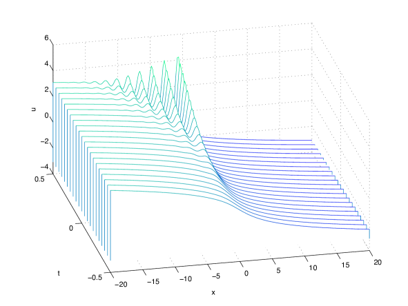
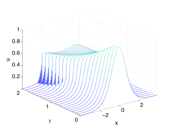
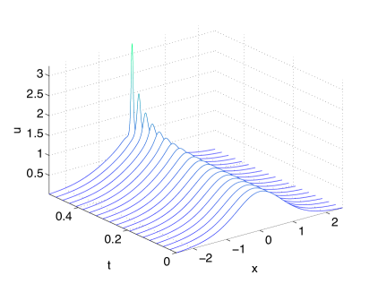
The existence of such solution to the P2Isuperscriptsubscriptabsent𝐼2{}_{I}^{2} equation has been conjectured in [43] (for T=0𝑇0T=0 such a conjecture gas already been formulated in [18]) and proved in [27]. See Figure 1 below for a plot of such solution in the (x,t)𝑥𝑡(x,t) plane.

Refer to caption
Figure 1: The special solution to the P2Isuperscriptsubscriptabsent𝐼2{}_{I}^{2} equation for several values of t𝑡t.

Recalling that the function U(X,T)𝑈𝑋𝑇U(X,T) satisfies the KdV equation

UT+UUX+112UXXX=0,subscript𝑈𝑇𝑈subscript𝑈𝑋112subscript𝑈𝑋𝑋𝑋0U_{T}+U\,U_{X}+\frac{1}{12}U_{XXX}=0, (3.34)

the asymptotic formulae (3.5) meet the following two conditions:

\bullet for t<t0𝑡subscript𝑡0t<t_{0} the solution (3.5) tends to the hodograph solution (3.2) as ϵ0italic-ϵ0\epsilon\to 0;

\bullet near the point of break-up the rescaled Riemann invariant rsubscript𝑟r_{-} approximately satisfies the KdV equation (3.27) while the rescaled Riemann invariant r+subscript𝑟r_{+} admits an approximate representation (3.28). Indeed, choosing

k=ϵ6/7𝑘superscriptitalic-ϵ67k=\epsilon^{6/7}

one obtains

ε=1.𝜀1\varepsilon=1.

So, after rescaling of the characteristic variables

X+=(122ρ2γ3β9)1/7X^+,X=(123ρ3γβ3)1/7X^formulae-sequencesubscript𝑋limit-fromsuperscriptsuperscript122superscript𝜌2superscript𝛾3superscript𝛽917^𝑋subscript𝑋superscriptsuperscript123superscript𝜌3𝛾superscript𝛽317subscript^𝑋X_{+}=\left(\frac{12^{2}\rho^{2}\gamma^{3}}{\beta^{9}}\right)^{1/7}\hat{X}+,\quad X_{-}=\left(\frac{12^{3}\rho^{3}\gamma}{\beta^{3}}\right)^{1/7}\hat{X}_{-}

one derives from (3.27) that the rescaled function

R^=(βγ212ρ)1/7Rsubscript^𝑅superscript𝛽superscript𝛾212𝜌17subscript𝑅\hat{R}_{-}=\left(\frac{\beta\,\gamma^{2}}{12\rho}\right)^{1/7}R_{-}

satisfies the normalized KdV equation (3.34),

R^X^++R^R^X^+1123R^X^3=0.subscript^𝑅subscript^𝑋subscript^𝑅subscript^𝑅subscript^𝑋112superscript3subscript^𝑅superscriptsubscript^𝑋30\frac{\partial\hat{R}_{-}}{\partial\hat{X}_{+}}+\hat{R}_{-}\frac{\partial\hat{R}_{-}}{\partial\hat{X}_{-}}+\frac{1}{12}\frac{\partial^{3}\hat{R}_{-}}{\partial\hat{X}_{-}^{3}}=0.

Moreover, for large X^subscript^𝑋\hat{X}_{-} and negative X^+subscript^𝑋\hat{X}_{+} it behaves like the root of the cubic equation

X^=X^+R^16R^3.subscript^𝑋subscript^𝑋subscript^𝑅16superscriptsubscript^𝑅3\hat{X}_{-}=\hat{X}_{+}\hat{R}_{-}-\frac{1}{6}\hat{R}_{-}^{3}.

The function

R^=U(X^,X^+)subscript^𝑅𝑈subscript^𝑋subscript^𝑋\hat{R}_{-}=U\left(\hat{X}_{-},\hat{X}_{+}\right)

is a solution to KdV satisfying these properties. Returning to the original variables r¯subscript¯𝑟\bar{r}_{-}, x¯±subscript¯𝑥plus-or-minus\bar{x}_{\pm} one arrives at the formula (3.5).

4 Elliptic case

In this section we study solutions to the system (1) when the unperturbed systems (2.16) is elliptic. We will restrict our analysis to analytic initial data. We first derive the generic singularity of the solution to the elliptic systems of the form (2.16) and then we study the local behaviour of the solution of the system (1) with ϵ>0italic-ϵ0\epsilon>0 near such a singularity. We argue that such behaviour in a double scaling limit is described by the tritronquée solution to the Painlevé I equation.

Let us now proceed to considering the elliptic case for the system (2.16), namely

huuhvv<0.subscript𝑢𝑢subscript𝑣𝑣0h_{uu}h_{vv}<0. (4.1)

The initial data u(x,0)𝑢𝑥0u(x,0) and v(x,0)𝑣𝑥0v(x,0) are analytic functions. The Riemann invariants

dr±=κ±(|hvv|dv±i|huu|du),κ=κ+formulae-sequence𝑑subscript𝑟plus-or-minussubscript𝜅plus-or-minusplus-or-minussubscript𝑣𝑣𝑑𝑣𝑖subscript𝑢𝑢𝑑𝑢subscript𝜅superscriptsubscript𝜅dr_{\pm}=\kappa_{\pm}\left(\sqrt{|h_{vv}|}\,dv\pm i\sqrt{|h_{uu}|}\,du\right),\quad\kappa_{-}=\kappa_{+}^{*} (4.2)

and the characteristic speeds

λ±=huv±isign (hvv)|huuhvv|.subscript𝜆plus-or-minusplus-or-minussubscript𝑢𝑣𝑖sign subscript𝑣𝑣subscript𝑢𝑢subscript𝑣𝑣\lambda_{\pm}=h_{uv}\pm i\,\mbox{sign}\hskip 1.42262pt(h_{vv})\sqrt{|h_{uu}h_{vv}|}. (4.3)

are complex conjugate (the asterisk will be used for the complex conjugation),

r=r+λ=λ+formulae-sequencesubscript𝑟superscriptsubscript𝑟subscript𝜆superscriptsubscript𝜆r_{-}=r_{+}^{*}\qquad\lambda_{-}=\lambda_{+}^{*}

At the point of elliptic break-up of a solution, written in the form (3), the following two complex conjugated equations hold

μ+,+0=λ+,+0t0superscriptsubscript𝜇0superscriptsubscript𝜆0subscript𝑡0\displaystyle\mu_{+,+}^{0}=\lambda_{+,+}^{0}t_{0}
(4.4)
μ,0=λ,0t0.superscriptsubscript𝜇0superscriptsubscript𝜆0subscript𝑡0\displaystyle\mu_{-,-}^{0}=\lambda_{-,-}^{0}t_{0}.

The characteristic variables at the point of catastrophe are defined as

x±=(xx0)+λ±0(tt0)subscript𝑥plus-or-minus𝑥subscript𝑥0superscriptsubscript𝜆plus-or-minus0𝑡subscript𝑡0x_{\pm}=(x-x_{0})+\lambda_{\pm}^{0}(t-t_{0}) (4.5)

and are also complex conjugate. One can represent the functions r±=r±(x,t)subscript𝑟plus-or-minussubscript𝑟plus-or-minus𝑥𝑡r_{\pm}=r_{\pm}(x,t) as functions of (x+,x)subscript𝑥subscript𝑥(x_{+},x_{-}). Let us redenote r¯±=r±(x+,x)r±0subscript¯𝑟plus-or-minussubscript𝑟plus-or-minussubscript𝑥subscript𝑥superscriptsubscript𝑟plus-or-minus0\bar{r}_{\pm}=r_{\pm}(x_{+},x_{-})-r_{\pm}^{0} the resulting shifted and transformed Riemann invariants.

Lemma 4.1

For a generic solution to the system (3) near a point of elliptic break-up the limits

R±(X±)=limk0k1/2r¯±(kX+,kX)subscript𝑅plus-or-minussubscript𝑋plus-or-minussubscript𝑘0superscript𝑘12subscript¯𝑟plus-or-minus𝑘subscript𝑋𝑘subscript𝑋R_{\pm}(X_{\pm})=\lim_{k\to 0}k^{-1/2}\bar{r}_{\pm}(k\,X_{+},k\,X_{-}) (4.6)

exist and satisfy the quadratic equation

X±=12a±R±2subscript𝑋plus-or-minus12subscript𝑎plus-or-minussuperscriptsubscript𝑅plus-or-minus2X_{\pm}=\frac{1}{2}a_{\pm}R_{\pm}^{2} (4.7)

with

x±=kX±,a±=μ±,±±0t0λ±,±±0.formulae-sequencesubscript𝑥plus-or-minus𝑘subscript𝑋plus-or-minussubscript𝑎plus-or-minussuperscriptsubscript𝜇plus-or-minusplus-or-minusabsentplus-or-minus0subscript𝑡0superscriptsubscript𝜆plus-or-minusplus-or-minusabsentplus-or-minus0x_{\pm}=kX_{\pm},\qquad a_{\pm}=\mu_{\pm,\pm\pm}^{0}-t_{0}\lambda_{\pm,\pm\pm}^{0}. (4.8)

In the sequel it will be assumed that

a±0subscript𝑎plus-or-minus0a_{\pm}\neq 0 (4.9)

(this condition will be added to the genericity assumptions).

Proof  Differentiating the hodograph relations (3) one obtains

μ+,tλ+,0,μ,+tλ,+0.formulae-sequencesubscript𝜇𝑡subscript𝜆0subscript𝜇𝑡subscript𝜆0\mu_{+,-}-t\,\lambda_{+,-}\equiv 0,\quad\mu_{-,+}-t\,\lambda_{-,+}\equiv 0.

Moreover, differentiating (3.8) one finds that

μ+,+tλ+,+=λ+,μ+,+tλ+,+λ+λsubscript𝜇absent𝑡subscript𝜆absentsubscript𝜆subscript𝜇𝑡subscript𝜆subscript𝜆subscript𝜆\displaystyle\mu_{+,+-}-t\,\lambda_{+,+-}=\lambda_{+,-}\frac{\mu_{+,+}-t\,\lambda_{+,+}}{\lambda_{+}-\lambda_{-}}
μ,+tλ,+=λ,+μ,tλ,λ+λsubscript𝜇absent𝑡subscript𝜆absentsubscript𝜆subscript𝜇𝑡subscript𝜆subscript𝜆subscript𝜆\displaystyle\mu_{-,+-}-t\,\lambda_{-,+-}=-\lambda_{-,+}\frac{\mu_{-,-}-t\,\lambda_{-,-}}{\lambda_{+}-\lambda_{-}}
μ+,tλ+,=λ+,μ,tλ,λ+λsubscript𝜇absent𝑡subscript𝜆absentsubscript𝜆subscript𝜇𝑡subscript𝜆subscript𝜆subscript𝜆\displaystyle\mu_{+,--}-t\,\lambda_{+,--}=-\lambda_{+,-}\frac{\mu_{-,-}-t\,\lambda_{-,-}}{\lambda_{+}-\lambda_{-}}
μ,++tλ,++=λ,+μ+,+tλ+,+λ+λ.subscript𝜇absent𝑡subscript𝜆absentsubscript𝜆subscript𝜇𝑡subscript𝜆subscript𝜆subscript𝜆\displaystyle\mu_{-,++}-t\,\lambda_{-,++}=\lambda_{-,+}\frac{\mu_{+,+}-t\,\lambda_{+,+}}{\lambda_{+}-\lambda_{-}}.

Hence, due to (4), all these combinations of the second derivatives vanish at the break-up point. Expanding the hodograph equations (3) in Taylor series near the point of catastrophe, one easily arrives at (4.7).    


Choosing Riemann invariants r±=r±(u,v)subscript𝑟plus-or-minussubscript𝑟plus-or-minus𝑢𝑣r_{\pm}=r_{\pm}(u,v) of the leading term as a system of coordinates on the space of dependent variables, and x±subscript𝑥plus-or-minusx_{\pm} as independent variables, the system (1) takes the form

tr+=λ+(r)xr++ϵ2[C++(r)x3r++C+(r)x3r+]+O(ϵ3)subscript𝑡subscript𝑟subscript𝜆𝑟subscript𝑥subscript𝑟superscriptitalic-ϵ2delimited-[]subscriptsuperscript𝐶𝑟superscriptsubscript𝑥3subscript𝑟subscriptsuperscript𝐶𝑟superscriptsubscript𝑥3subscript𝑟𝑂superscriptitalic-ϵ3\displaystyle\partial_{t}r_{+}=\lambda_{+}(r)\partial_{x}r_{+}+\epsilon^{2}\left[C^{+}_{+}(r)\partial_{x}^{3}r_{+}+C^{+}_{-}(r)\partial_{x}^{3}r_{-}+\dots\right]+O\left(\epsilon^{3}\right)
(4.10)
tr=λ(r)xr+ϵ2[C+(r)x3r++C(r)x3r+]+O(ϵ3)subscript𝑡subscript𝑟subscript𝜆𝑟subscript𝑥subscript𝑟superscriptitalic-ϵ2delimited-[]subscriptsuperscript𝐶𝑟superscriptsubscript𝑥3subscript𝑟subscriptsuperscript𝐶𝑟superscriptsubscript𝑥3subscript𝑟𝑂superscriptitalic-ϵ3\displaystyle\partial_{t}r_{-}=\lambda_{-}(r)\partial_{x}r_{-}+\epsilon^{2}\left[C^{-}_{+}(r)\partial_{x}^{3}r_{+}+C^{-}_{-}(r)\partial_{x}^{3}r_{-}+\dots\right]+O\left(\epsilon^{3}\right)

with

C++=ahvv+2ib|huuhvv|+chuu2i|huuhvv|,C+=κ+κchuuahvv2i|huuhvv|\displaystyle C_{+}^{+}=\frac{a\,h_{vv}+2ib\,\sqrt{|h_{uu}h_{vv}|}+c\,h_{uu}}{2i\sqrt{|h_{uu}h_{vv}}|},\quad C_{-}^{+}=\frac{\kappa_{+}}{\kappa_{-}}\frac{c\,h_{uu}-a\,h_{vv}}{2i\sqrt{|h_{uu}h_{vv}}|}
(4.11)
C+=κκ+ahvvchuu2i|huuhvv|,C=ahvv2ib|huuhvv|+chuu2i|huuhvv|.\displaystyle C_{+}^{-}=\frac{\kappa_{-}}{\kappa_{+}}\frac{a\,h_{vv}-c\,h_{uu}}{2i\sqrt{|h_{uu}h_{vv}}|},\quad C_{-}^{-}=-\frac{a\,h_{vv}-2ib\,\sqrt{|h_{uu}h_{vv}|}+c\,h_{uu}}{2i\sqrt{|h_{uu}h_{vv}}|}.

As above we will denote r¯±=r¯±(x+,x;ϵ)subscript¯𝑟plus-or-minussubscript¯𝑟plus-or-minussubscript𝑥subscript𝑥italic-ϵ\bar{r}_{\pm}=\bar{r}_{\pm}(x_{+},x_{-};\epsilon) a shifted generic solution to the system (4) with ϵitalic-ϵ\epsilon-independent initial data written as functions of the complex conjugated linearized characteristic variables (4.5). Like above we will be interested in the multiscale expansion of these complex conjugated functions

r¯±(x¯+,x¯;ϵ)=k1/2R±(X+,X;ε)+kΔR±(X+,X;ε)+𝒪(k3/2)subscript¯𝑟plus-or-minussubscript¯𝑥subscript¯𝑥italic-ϵsuperscript𝑘12subscript𝑅plus-or-minussubscript𝑋subscript𝑋𝜀𝑘Δsubscript𝑅plus-or-minussubscript𝑋subscript𝑋𝜀𝒪superscript𝑘32\displaystyle\bar{r}_{\pm}(\bar{x}_{+},\bar{x}_{-};\epsilon)=k^{1/2}R_{\pm}\left(X_{+},X_{-};\varepsilon\right)+k\,\Delta R_{\pm}\left(X_{+},X_{-};\varepsilon\right)+{\mathcal{O}}\left(k^{3/2}\right) (4.12)
x±=kX±,ϵ=k5/4ε,k0.formulae-sequencesubscript𝑥plus-or-minus𝑘subscript𝑋plus-or-minusformulae-sequenceitalic-ϵsuperscript𝑘54𝜀𝑘0\displaystyle x_{\pm}=k\,X_{\pm},\quad\epsilon=k^{5/4}\varepsilon,\quad k\to 0.

We will now show that existence of such expansions implies that the leading term is a holomorphic/antiholomorphic function

R±X=0subscript𝑅plus-or-minussubscript𝑋minus-or-plus0\dfrac{\partial R_{\pm}}{\partial X_{\mp}}=0

satisfying an ODE.

Theorem 4.2

Let r±(x,t,;ϵ)r_{\pm}(x,t,;\epsilon) be a solution of the system (4) such that there exist the limits

R±(X+,X;ε)=limk0k12r¯±(kX+,kX;k54ε)ΔR±(X+,X;ε)=limk0r¯±(kX+,kX;k54ε)k12R±(X+,X;ε)ksubscript𝑅plus-or-minussubscript𝑋subscript𝑋𝜀subscript𝑘0superscript𝑘12subscript¯𝑟plus-or-minus𝑘subscript𝑋𝑘subscript𝑋superscript𝑘54𝜀Δsubscript𝑅plus-or-minussubscript𝑋subscript𝑋𝜀subscript𝑘0subscript¯𝑟plus-or-minus𝑘subscript𝑋𝑘subscript𝑋superscript𝑘54𝜀superscript𝑘12subscript𝑅plus-or-minussubscript𝑋subscript𝑋𝜀𝑘\begin{split}R_{\pm}(X_{+},X_{-};\varepsilon)&=\lim_{k\rightarrow 0}k^{-\frac{1}{2}}\bar{r}_{\pm}(kX_{+},kX_{-};k^{\frac{5}{4}}\varepsilon)\\ \Delta R_{\pm}(X_{+},X_{-};\varepsilon)&=\lim_{k\rightarrow 0}\dfrac{\bar{r}_{\pm}(kX_{+},kX_{-};k^{\frac{5}{4}}\varepsilon)-k^{\frac{1}{2}}R_{\pm}(X_{+},X_{-};\varepsilon)}{k}\end{split} (4.13)

Then the function R+=R+(X+,X;ε)subscript𝑅subscript𝑅subscript𝑋subscript𝑋𝜀R_{+}=R_{+}(X_{+},X_{-};\varepsilon) satisfies the Cauchy–Riemann equation

R+(X+,X;ε)X=0subscript𝑅subscript𝑋subscript𝑋𝜀subscript𝑋0\dfrac{\partial R_{+}(X_{+},X_{-};\varepsilon)}{\partial X_{-}}=0 (4.14)

and also the equation

λ+,+0R+R+X++ε2C++(r0)3R+X+3=c+superscriptsubscript𝜆0subscript𝑅subscript𝑅subscript𝑋superscript𝜀2superscriptsubscript𝐶superscript𝑟0superscript3subscript𝑅subscriptsuperscript𝑋3subscript𝑐\lambda_{+,+}^{0}R_{+}\dfrac{\partial R_{+}}{\partial X_{+}}+\varepsilon^{2}C_{+}^{+}(r^{0})\dfrac{\partial^{3}R_{+}}{\partial X^{3}_{+}}=c_{+} (4.15)

where c+subscript𝑐c_{+} is a holomorphic function of X+subscript𝑋X_{+} such that

c+(X+)=λ+,+0a++O(1/X+δ),asX+andδ>0.formulae-sequencesubscript𝑐subscript𝑋subscriptsuperscript𝜆0subscript𝑎𝑂1superscriptsubscript𝑋𝛿asformulae-sequencesubscript𝑋and𝛿0c_{+}(X_{+})=\dfrac{\lambda^{0}_{+,+}}{a_{+}}+O(1/X_{+}^{\delta}),\;\;\mbox{\rm as}\quad X_{+}\rightarrow\infty\quad\mbox{\rm and}\quad\delta>0. (4.16)

Here C++subscriptsuperscript𝐶C^{+}_{+} has been defined in (4). The function R=R(X;ε)subscript𝑅subscript𝑅subscript𝑋𝜀R_{-}=R_{-}(X_{-};\varepsilon) is antiholomorphic and satisfies the complex conjugate of (4.15). The function ΔR+(X+,X;ε)Δsubscript𝑅subscript𝑋subscript𝑋𝜀\Delta R_{+}(X_{+},X_{-};\varepsilon) satisfies the equation

(λ0λ+0)XΔR+=λ+,0RR+X++ε2C+(r0)3RX3+c+,superscriptsubscript𝜆0superscriptsubscript𝜆0subscript𝑋Δsubscript𝑅superscriptsubscript𝜆0subscript𝑅subscript𝑅subscript𝑋superscript𝜀2superscriptsubscript𝐶superscript𝑟0superscript3subscript𝑅superscriptsubscript𝑋3subscript𝑐(\lambda_{-}^{0}-\lambda_{+}^{0})\dfrac{\partial}{\partial X_{-}}\Delta R_{+}=\lambda_{+,-}^{0}R_{-}\dfrac{\partial R_{+}}{\partial X_{+}}+\varepsilon^{2}C_{-}^{+}(r^{0})\dfrac{\partial^{3}R_{-}}{\partial X_{-}^{3}}+c_{+}, (4.17)

where C+subscriptsuperscript𝐶C^{+}_{-} has been defined in (4). The function ΔR(X+,X;ε)Δsubscript𝑅subscript𝑋subscript𝑋𝜀\Delta R_{-}(X_{+},X_{-};\varepsilon) satisfies the complex conjugate of the above equation.

Proof In order to prove the theorem it is sufficient to plug the expansion (4.12) and (4.13) into equation (4) giving the following expansions

k1/2(λ+0λ0)R+X+(λ+0λ0)ΔR+X+(λ+,+0R++λ+,0R)(X++X)R++ε2C++(r0)(X++X)3R++ε2C+(r0)(X++X)3R=𝒪(k1/2)k1/2(λ0λ+0)RX++(λ0λ+0)ΔRX++(λ,+0R++λ,0R)(X++X)R+ε2C+(r0)(X++X)3R++ε2C(r0)(X++X)3R=𝒪(k1/2)superscript𝑘12superscriptsubscript𝜆0superscriptsubscript𝜆0subscript𝑅subscript𝑋superscriptsubscript𝜆0superscriptsubscript𝜆0Δsubscript𝑅subscript𝑋superscriptsubscript𝜆0subscript𝑅superscriptsubscript𝜆0subscript𝑅subscript𝑋subscript𝑋subscript𝑅superscript𝜀2superscriptsubscript𝐶superscript𝑟0superscriptsubscript𝑋subscript𝑋3subscript𝑅superscript𝜀2superscriptsubscript𝐶superscript𝑟0superscriptsubscript𝑋subscript𝑋3subscript𝑅𝒪superscript𝑘12superscript𝑘12superscriptsubscript𝜆0superscriptsubscript𝜆0subscript𝑅subscript𝑋superscriptsubscript𝜆0superscriptsubscript𝜆0Δsubscript𝑅subscript𝑋superscriptsubscript𝜆0subscript𝑅superscriptsubscript𝜆0subscript𝑅subscript𝑋subscript𝑋subscript𝑅superscript𝜀2superscriptsubscript𝐶superscript𝑟0superscriptsubscript𝑋subscript𝑋3subscript𝑅superscript𝜀2superscriptsubscript𝐶superscript𝑟0superscriptsubscript𝑋subscript𝑋3subscript𝑅𝒪superscript𝑘12\begin{split}&k^{-1/2}\left(\lambda_{+}^{0}-\lambda_{-}^{0}\right)\frac{\partial R_{+}}{\partial X_{-}}+\left(\lambda_{+}^{0}-\lambda_{-}^{0}\right)\frac{\partial\Delta R_{+}}{\partial X_{-}}+\left(\lambda_{+,+}^{0}R_{+}+\lambda_{+,-}^{0}R_{-}\right)\left(\frac{\partial}{\partial X_{+}}+\frac{\partial}{\partial X_{-}}\right)R_{+}\\ &+\varepsilon^{2}C_{+}^{+}(r^{0})\left(\frac{\partial}{\partial X_{+}}+\frac{\partial}{\partial X_{-}}\right)^{3}R_{+}+\varepsilon^{2}C_{+}^{-}(r^{0})\left(\frac{\partial}{\partial X_{+}}+\frac{\partial}{\partial X_{-}}\right)^{3}R_{-}={\mathcal{O}}\left(k^{1/2}\right)\\ &k^{-1/2}\left(\lambda_{-}^{0}-\lambda_{+}^{0}\right)\frac{\partial R_{-}}{\partial X_{+}}+\left(\lambda_{-}^{0}-\lambda_{+}^{0}\right)\frac{\partial\Delta R_{-}}{\partial X_{+}}+\left(\lambda_{-,+}^{0}R_{+}+\lambda_{-,-}^{0}R_{-}\right)\left(\frac{\partial}{\partial X_{+}}+\frac{\partial}{\partial X_{-}}\right)R_{-}\\ &+\varepsilon^{2}C_{-}^{+}(r^{0})\left(\frac{\partial}{\partial X_{+}}+\frac{\partial}{\partial X_{-}}\right)^{3}R_{+}+\varepsilon^{2}C_{-}^{-}(r^{0})\left(\frac{\partial}{\partial X_{+}}+\frac{\partial}{\partial X_{-}}\right)^{3}R_{-}={\mathcal{O}}\left(k^{1/2}\right)\end{split} (4.18)

Since λ+0λ0superscriptsubscript𝜆0superscriptsubscript𝜆0\lambda_{+}^{0}\neq\lambda_{-}^{0}, from the leading term it readily follows that

R+X=0,RX+=0.formulae-sequencesubscript𝑅subscript𝑋0subscript𝑅subscript𝑋0\frac{\partial R_{+}}{\partial X_{-}}=0,\quad\frac{\partial R_{-}}{\partial X_{+}}=0. (4.19)

Separating holomorphic and antiholomorphic parts in the terms of order 𝒪(1)𝒪1{\mathcal{O}}(1) one arrives at equations (4.15), (4.17) and their complex conjugates.

Equation (4.15) must have a solution with asymptotic behaviour determined by (4.7), namely

R+(X+)±2X+a+,asX+.formulae-sequencesubscript𝑅subscript𝑋plus-or-minus2subscript𝑋subscript𝑎assubscript𝑋R_{+}(X_{+})\rightarrow\pm\sqrt{\dfrac{2X_{+}}{a_{+}}},\quad\mbox{as}\;\;X_{+}\rightarrow\infty. (4.20)

This immediately gives that c+subscript𝑐c_{+} is an analytic function of X+subscript𝑋X_{+} with asymptotic behavior at infinity

c+(X+)=λ+,+0a++O(1/X+δ),δ>0c(X)=c¯+(X¯+).formulae-sequencesubscript𝑐subscript𝑋subscriptsuperscript𝜆0subscript𝑎𝑂1superscriptsubscript𝑋𝛿formulae-sequence𝛿0subscript𝑐subscript𝑋subscript¯𝑐subscript¯𝑋c_{+}(X_{+})=\dfrac{\lambda^{0}_{+,+}}{a_{+}}+O(1/X_{+}^{\delta}),\;\;\delta>0\quad c_{-}(X_{-})=\bar{c}_{+}(\bar{X}_{+}). (4.21)

\square

Assuming c+=constsubscript𝑐constc_{+}={\rm const} we arrive at an ODE for the function R+=R+(X+)subscript𝑅subscript𝑅subscript𝑋R_{+}=R_{+}(X_{+}) equivalent to the Painlevé-I equation,

ε2C++(r0)R+′′+12λ+,+0R+2=λ+,+0a+,superscript𝜀2superscriptsubscript𝐶subscript𝑟0superscriptsubscript𝑅′′12superscriptsubscript𝜆0superscriptsubscript𝑅2superscriptsubscript𝜆0subscript𝑎\varepsilon^{2}C_{+}^{+}(r_{0})R_{+}^{\prime\prime}+\frac{1}{2}\lambda_{+,+}^{0}R_{+}^{2}=\frac{\lambda_{+,+}^{0}}{a_{+}}, (4.22)

with asymptotic behaviour (4.20). The complex conjugate of the above equation gives the corresponding Painlevé-I equation for R=R(X)subscript𝑅subscript𝑅subscript𝑋R_{-}=R_{-}(X_{-}). If we linearized the increments of the Riemann invariants we obtain

r±r±0=κ±0(|hvv0|(vv0)±i|huu0|(uu0))+O(ϵ45).subscript𝑟plus-or-minussubscriptsuperscript𝑟0plus-or-minussubscriptsuperscript𝜅0plus-or-minusplus-or-minussubscriptsuperscript0𝑣𝑣𝑣subscript𝑣0𝑖subscriptsuperscript0𝑢𝑢𝑢subscript𝑢0𝑂superscriptitalic-ϵ45r_{\pm}-r^{0}_{\pm}=\kappa^{0}_{\pm}\left(\sqrt{|h^{0}_{vv}|}\,(v-v_{0})\pm i\sqrt{|h^{0}_{uu}|}\,(u-u_{0})\right)+O(\epsilon^{\frac{4}{5}}). (4.23)

For simplicity we normalize the constant κ±0subscriptsuperscript𝜅0plus-or-minus\kappa^{0}_{\pm} to

κ+0=κ0={1,huu0<0andhvv0>01,huu0>0andhvv0<0.superscriptsubscript𝜅0superscriptsubscript𝜅0cases1superscriptsubscript𝑢𝑢0expectation0andsuperscriptsubscript𝑣𝑣001superscriptsubscript𝑢𝑢00andsuperscriptsubscript𝑣𝑣00\kappa_{+}^{0}=\kappa_{-}^{0}=\left\{\begin{array}[]{rl}1,&h_{uu}^{0}<0~{}\mbox{and}~{}h_{vv}^{0}>0\\ \sqrt{-1},&h_{uu}^{0}>0~{}\mbox{and}~{}h_{vv}^{0}<0.\end{array}\right. (4.24)

From (4.22) and (4.23) we arrive at the following

Conjecture 4.3

The functions u(x,t,ϵ)𝑢𝑥𝑡italic-ϵu(x,t,\epsilon) and v(x,t,ϵ)𝑣𝑥𝑡italic-ϵv(x,t,\epsilon) that solves the system (1) admits the following asymptotic representation in the double scaling limit xx0𝑥subscript𝑥0x\rightarrow x_{0}, tt0𝑡subscript𝑡0t\rightarrow t_{0} and ϵ0italic-ϵ0\epsilon\rightarrow 0 in such a way that

xx0+λ±0(tt0)ϵ45𝑥subscript𝑥0subscriptsuperscript𝜆0plus-or-minus𝑡subscript𝑡0superscriptitalic-ϵ45\dfrac{x-x_{0}+\lambda^{0}_{\pm}(t-t_{0})}{\epsilon^{\frac{4}{5}}} (4.25)

remains bounded

|hvv0|(v(x,t,ϵ)v0)+i|huu0|(u(x,t,ϵ)u0)=12(ϵ2C++(u0,v0)(12a+)2λ+,+0)15Ω(ξ)+O(ϵ45),subscriptsuperscript0𝑣𝑣𝑣𝑥𝑡italic-ϵsubscript𝑣0𝑖subscriptsuperscript0𝑢𝑢𝑢𝑥𝑡italic-ϵsubscript𝑢012superscriptsuperscriptitalic-ϵ2superscriptsubscript𝐶subscript𝑢0subscript𝑣0superscript12subscript𝑎2superscriptsubscript𝜆015Ω𝜉𝑂superscriptitalic-ϵ45\sqrt{|h^{0}_{vv}|}\,(v(x,t,\epsilon)-v_{0})+i\sqrt{|h^{0}_{uu}|}\,(u(x,t,\epsilon)-u_{0})=-12\left(\dfrac{\epsilon^{2}C_{+}^{+}(u_{0},v_{0})}{(12a_{+})^{2}\lambda_{+,+}^{0}}\right)^{\frac{1}{5}}\Omega(\xi)+O(\epsilon^{\frac{4}{5}}), (4.26)

where

ξ=((λ+,+0)212a+ϵ4(C++(u0,v0))2)15(xx0+λ+0(tt0))𝜉superscriptsuperscriptsuperscriptsubscript𝜆0212subscript𝑎superscriptitalic-ϵ4superscriptsuperscriptsubscript𝐶subscript𝑢0subscript𝑣0215𝑥subscript𝑥0superscriptsubscript𝜆0𝑡subscript𝑡0\xi=\left(\dfrac{(\lambda_{+,+}^{0})^{2}}{12a_{+}\epsilon^{4}(C_{+}^{+}(u_{0},v_{0}))^{2}}\right)^{\frac{1}{5}}(x-x_{0}+\lambda_{+}^{0}(t-t_{0})) (4.27)

where a+subscript𝑎a_{+} and C++(u0,v0)superscriptsubscript𝐶subscript𝑢0subscript𝑣0C_{+}^{+}(u_{0},v_{0}) have been defined in (4.8) and (4) respectively and Ω=Ω(ξ)ΩΩ𝜉\Omega=\Omega(\xi) is the tritronquée solution to the Painlevé-I equation

Ωξξ=6Ω2ξ,subscriptΩ𝜉𝜉6superscriptΩ2𝜉\Omega_{\xi\xi}=6\Omega^{2}-\xi, (4.28)

determined uniquely by the asymptotic conditions333Note that there are additional tritronquée solutions ΩnsubscriptΩ𝑛\Omega_{n}, n=±1,±2𝑛plus-or-minus1plus-or-minus2n=\pm 1,\pm 2, related to ΩΩ\Omega via Ωn(ξ)=e4πi5Ω(e2πi5ξ)subscriptΩ𝑛𝜉superscript𝑒4𝜋𝑖5Ωsuperscript𝑒2𝜋𝑖5𝜉\Omega_{n}(\xi)=e^{\frac{4\pi i}{5}}\Omega(e^{\frac{2\pi i}{5}}\xi).

Ω(ξ)ξ6,|ξ|,|argξ|<45π.formulae-sequencesimilar-to-or-equalsΩ𝜉𝜉6formulae-sequence𝜉𝜉45𝜋\Omega(\xi)\simeq-\sqrt{\dfrac{\xi}{6}},\quad|\xi|\rightarrow\infty,\quad|\arg\xi|<\dfrac{4}{5}\pi. (4.29)

The smoothness of the solution of (4.28) with asymptotic condition (4.29) in a sector of the complex z𝑧z-plane of angle |argz|<4π/5𝑧4𝜋5|\arg z|<4\pi/5 conjectured in [46] has only recently been proved in [30]. For a plot of such solution in the complex plane see [46].

Remark 4.4

Observe that the tritronquée solution to the Painlevé-I equation is invariant with respect to complex conjugation

Ω(ξ¯)¯=Ω(ξ).¯Ω¯𝜉Ω𝜉\overline{\Omega\left(\bar{\xi}\right)}=\Omega(\xi). (4.30)

So the asymptotic representation of the linearised Riemann invariant |hvv0|(v(x,t,ϵ)v0)i|huu0|(u(x,t,ϵ)u0)subscriptsuperscript0𝑣𝑣𝑣𝑥𝑡italic-ϵsubscript𝑣0𝑖subscriptsuperscript0𝑢𝑢𝑢𝑥𝑡italic-ϵsubscript𝑢0\sqrt{|h^{0}_{vv}|}\,(v(x,t,\epsilon)-v_{0})-i\sqrt{|h^{0}_{uu}|}\,(u(x,t,\epsilon)-u_{0}) is given by the complex conjugate of (4.26).

Remark 4.5

We write the constant a+subscript𝑎a_{+} in the form

1a+=i(C++λ+,+0)2qeiψ,1subscript𝑎𝑖superscriptsubscriptsuperscript𝐶superscriptsubscript𝜆02𝑞superscript𝑒𝑖𝜓\dfrac{1}{a_{+}}=i\left(\dfrac{C^{+}_{+}}{\lambda_{+,+}^{0}}\right)^{2}qe^{i\psi},

with q>0𝑞0q>0 and ψ[π,π]𝜓𝜋𝜋\psi\in[-\pi,\pi]. One can check that when ψ=0𝜓0\psi=0 and t=t0𝑡subscript𝑡0t=t_{0} the quantity ξ𝜉\xi defined in (4.27) has to be purely imaginary, and this gives a rule for the selection of the fifth root, namely

ξ=i(qeiψ12ϵ4)15(xx0+λ+0(tt0)).𝜉𝑖superscript𝑞superscript𝑒𝑖𝜓12superscriptitalic-ϵ415𝑥subscript𝑥0superscriptsubscript𝜆0𝑡subscript𝑡0\xi=i\left(\dfrac{qe^{i\psi}}{12\epsilon^{4}}\right)^{\frac{1}{5}}(x-x_{0}+\lambda_{+}^{0}(t-t_{0})).

Note that the angle of the line ξ=ξ(xx0)𝜉𝜉𝑥subscript𝑥0\xi=\xi(x-x_{0}) for fixed t𝑡t, is equal to π2+ψ5𝜋2𝜓5\dfrac{\pi}{2}+\dfrac{\psi}{5} with ψ[π,π]𝜓𝜋𝜋\psi\in[-\pi,\pi], thus the maximal value of argξ𝜉\arg\xi is equal to 710π<45π710𝜋45𝜋\dfrac{7}{10}\pi<\dfrac{4}{5}\pi.

In the next subsection we consider an alternative derivation of the PI equation for a subclass of Hamiltonian PDEs having the structure of a generalized nonlinear Schrödinger equation.

4.1 Painlevé-I equation and almost integrable PDEs

In this subsection we give a different derivation of the conjecture 4.3 for Hamiltonian equations (2.16) with Hamiltonian H0=h(u,v)𝑑xsubscript𝐻0𝑢𝑣differential-d𝑥H_{0}=\int h(u,v)\,dx satisfying equation

huu=P′′(u)hvvsubscript𝑢𝑢superscript𝑃′′𝑢subscript𝑣𝑣h_{uu}=P^{\prime\prime}(u)h_{vv} (4.31)

for some smooth function P(u)𝑃𝑢P(u), with P′′(u)<0superscript𝑃′′𝑢0P^{\prime\prime}(u)<0. We will see below that, in particular, a very general family of nonlinear Schrödinger equations belongs to this subclass. The condition

huuhvv=P′′(u)<0subscript𝑢𝑢subscript𝑣𝑣superscript𝑃′′𝑢0\dfrac{h_{uu}}{h_{vv}}=P^{\prime\prime}(u)<0 (4.32)

guarantees that the unperturbed quasi-linear system is elliptic.

A local solution of the system (1) with h(u,v)𝑢𝑣h(u,v) satisfying (4.31) for given analytic initial data u0(x)subscript𝑢0𝑥u_{0}(x), v0(x)subscript𝑣0𝑥v_{0}(x) takes the form

x+thuv=futhvv=fv𝑥𝑡subscript𝑢𝑣subscript𝑓𝑢𝑡subscript𝑣𝑣subscript𝑓𝑣\begin{split}x+&th_{uv}=f_{u}\\ &th_{vv}=f_{v}\end{split} (4.33)

where the function f=f(u,v)𝑓𝑓𝑢𝑣f=f(u,v) satisfies equation

fuu=P′′(u)fvvsubscript𝑓𝑢𝑢superscript𝑃′′𝑢subscript𝑓𝑣𝑣f_{uu}=P^{\prime\prime}(u)f_{vv} (4.34)

and the condition

x=fu(u0(x),v0(x)),0=fv(u0(x),u0(x)).formulae-sequence𝑥subscript𝑓𝑢subscript𝑢0𝑥subscript𝑣0𝑥0subscript𝑓𝑣subscript𝑢0𝑥subscript𝑢0𝑥x=f_{u}(u_{0}(x),v_{0}(x)),\quad 0=f_{v}(u_{0}(x),u_{0}(x)). (4.35)

The equation for determining the point of elliptic umbilic catastrophe characterized by equation (4) in the variables u𝑢u and v𝑣v takes the form

huvvt0fuv0=0hvvv0t0fvv0=0subscript𝑢𝑣𝑣subscript𝑡0superscriptsubscript𝑓𝑢𝑣00subscriptsuperscript0𝑣𝑣𝑣subscript𝑡0superscriptsubscript𝑓𝑣𝑣00\begin{split}h_{uvv}t_{0}-f_{uv}^{0}&=0\\ h^{0}_{vvv}t_{0}-f_{vv}^{0}&=0\end{split} (4.36)

and the constants a±subscript𝑎plus-or-minusa_{\pm} takes the form

a±=fuvv0t0huvvvv0±i|P′′(u0)|(fvvv0t0hvvvv0).subscript𝑎plus-or-minusplus-or-minussubscriptsuperscript𝑓0𝑢𝑣𝑣subscript𝑡0superscriptsubscript𝑢𝑣𝑣𝑣𝑣0𝑖superscript𝑃′′subscript𝑢0superscriptsubscript𝑓𝑣𝑣𝑣0subscript𝑡0superscriptsubscript𝑣𝑣𝑣𝑣0a_{\pm}=f^{0}_{uvv}-t_{0}h_{uvvvv}^{0}\pm i\sqrt{|P^{\prime\prime}(u_{0})|}(f_{vvv}^{0}-t_{0}h_{vvvv}^{0}). (4.37)

To study the critical behaviour of solutions of (2) we first restrict ourselves to the almost integrable cases and recall some results in [44]. We describe Hamiltonian integrable perturbations of equation (2.16) up to terms of order O(ϵ3)𝑂superscriptitalic-ϵ3O(\epsilon^{3}).

Theorem 4.6

[44] Any Hamiltonian perturbation integrable up to order ϵ3superscriptitalic-ϵ3\epsilon^{3} of the system of equations (2.16) satisfying (4.31) is given by equations

ut=xδHhδv(x)vt=xδHhδu(x)subscript𝑢𝑡subscript𝑥𝛿subscript𝐻𝛿𝑣𝑥subscript𝑣𝑡subscript𝑥𝛿subscript𝐻𝛿𝑢𝑥\begin{split}u_{t}&=\partial_{x}\frac{\delta H_{h}}{\delta v(x)}\\ v_{t}&=\partial_{x}\frac{\delta H_{h}}{\delta u(x)}\end{split} (4.38)

with Hamiltonian Hh=Dh𝑑xsubscript𝐻𝐷differential-d𝑥H_{h}=\int Dh\,dx and Hamiltonian density Dh𝐷Dh given by

Dh=hϵ22{[P′′(ρuhvvv+ρvhuvv)+12P′′′ρvhvv]ux2+2(P′′ρvhvvv+ρuhuvv+P′′′4P′′ρuhvv)uxvx+(ρuhvvv+ρvhuvv)vx2+s3(vx2P′′ux2)hvv}+𝒪(ϵ3),𝐷superscriptitalic-ϵ22delimited-[]superscript𝑃′′subscript𝜌𝑢subscript𝑣𝑣𝑣subscript𝜌𝑣subscript𝑢𝑣𝑣12superscript𝑃′′′subscript𝜌𝑣subscript𝑣𝑣superscriptsubscript𝑢𝑥22superscript𝑃′′subscript𝜌𝑣subscript𝑣𝑣𝑣subscript𝜌𝑢subscript𝑢𝑣𝑣superscript𝑃′′′4superscript𝑃′′subscript𝜌𝑢subscript𝑣𝑣subscript𝑢𝑥subscript𝑣𝑥subscript𝜌𝑢subscript𝑣𝑣𝑣subscript𝜌𝑣subscript𝑢𝑣𝑣superscriptsubscript𝑣𝑥2subscript𝑠3superscriptsubscript𝑣𝑥2superscript𝑃′′superscriptsubscript𝑢𝑥2subscript𝑣𝑣𝒪superscriptitalic-ϵ3\begin{split}Dh&=h-\frac{\epsilon^{2}}{2}\left\{\left[P^{\prime\prime}(\rho_{u}h_{vvv}+\rho_{v}h_{uvv})+\frac{1}{2}P^{\prime\prime\prime}\rho_{v}h_{vv}\right]\,u_{x}^{2}\right.\\ &+2\left(P^{\prime\prime}\rho_{v}h_{vvv}+\rho_{u}h_{uvv}+\frac{P^{\prime\prime\prime}}{4P^{\prime\prime}}\rho_{u}h_{vv}\right)\,u_{x}v_{x}\\ &\left.+\left(\rho_{u}h_{vvv}+\rho_{v}h_{uvv}\right)\,v_{x}^{2}+s_{3}\,\left(v_{x}^{2}-P^{\prime\prime}u_{x}^{2}\right)\,h_{vv}\right\}+{\mathcal{O}}\left(\epsilon^{3}\right),\end{split} (4.39)

where the function ρ=ρ(u,v)𝜌𝜌𝑢𝑣\rho=\rho(u,v) satisfies the linear PDE

ρuuP′′ρvv=P′′′2P′′ρusubscript𝜌𝑢𝑢superscript𝑃′′subscript𝜌𝑣𝑣superscript𝑃′′′2superscript𝑃′′subscript𝜌𝑢\rho_{uu}-P^{\prime\prime}\rho_{vv}=\frac{P^{\prime\prime\prime}}{2P^{\prime\prime}}\,\rho_{u} (4.40)

and s3=s3(u,v)subscript𝑠3subscript𝑠3𝑢𝑣s_{3}=s_{3}(u,v) is an arbitrary function. For any function f=f(u,v)𝑓𝑓𝑢𝑣f=f(u,v) that satisfies (4.34) the corresponding Hamiltonian Hfsubscript𝐻𝑓H_{f} given by an equivalent expression to (4.39), Poisson commute with Hhsubscript𝐻H_{h} up to ϵ3superscriptitalic-ϵ3\epsilon^{3}, namely

{Hh,Hf}=O(ϵ3).subscript𝐻subscript𝐻𝑓𝑂superscriptitalic-ϵ3\{H_{h},\,H_{f}\}=O(\epsilon^{3}).

Furthermore, a class of solutions of the system (4.38) characterized by an analogue of the string equation is given by the following theorem.

Theorem 4.7

[44] The solutions to the string equation

x+tδHhδu(x)=δHfδu(x)𝑥𝑡𝛿subscript𝐻superscript𝛿𝑢𝑥𝛿subscript𝐻𝑓𝛿𝑢𝑥\displaystyle x+t\,\frac{\delta H_{h^{\prime}}}{\delta u(x)}=\frac{\delta H_{f}}{\delta u(x)}
(4.41)
tδHhδv(x)=δHfδv(x)𝑡𝛿subscript𝐻superscript𝛿𝑣𝑥𝛿subscript𝐻𝑓𝛿𝑣𝑥\displaystyle\qquad t\,\frac{\delta H_{h^{\prime}}}{\delta v(x)}=\frac{\delta H_{f}}{\delta v(x)}

also solve the Hamiltonian equations

ut=xδHhδv(x)subscript𝑢𝑡subscript𝑥𝛿subscript𝐻𝛿𝑣𝑥\displaystyle u_{t}=\partial_{x}\frac{\delta H_{h}}{\delta v(x)}
(4.42)
vt=xδHhδu(x)subscript𝑣𝑡subscript𝑥𝛿subscript𝐻𝛿𝑢𝑥\displaystyle v_{t}=\partial_{x}\frac{\delta H_{h}}{\delta u(x)}

where f=f(u,v)𝑓𝑓𝑢𝑣f=f(u,v) is another solution to fuu=P′′(u)fvvsubscript𝑓𝑢𝑢superscript𝑃′′𝑢subscript𝑓𝑣𝑣f_{uu}=P^{\prime\prime}(u)f_{vv}, and

h:=hv.assignsuperscript𝑣h^{\prime}:=\frac{\partial h}{\partial v}.

We remark that (4.7) is a system of couple ODEs for u𝑢u and v𝑣v having t𝑡t has a parameter.

We can apply to the system (4.7) the rescaling (4.12). Let us first introduce the Riemann invariants for the Hamiltonians H0subscript𝐻0H_{0} satisfying (4.31)

r±=v±iQ(u),Q(u)=P′′(u).formulae-sequencesubscript𝑟plus-or-minusplus-or-minus𝑣𝑖𝑄𝑢superscript𝑄𝑢superscript𝑃′′𝑢r_{\pm}=v\pm iQ(u),\quad Q^{\prime}(u)=\sqrt{P^{\prime\prime}(u)}.

Choosing the Riemann invariants r±=r±(u,v)subscript𝑟plus-or-minussubscript𝑟plus-or-minus𝑢𝑣r_{\pm}=r_{\pm}(u,v) as a systems of coordinates on the space of dependent variables one can write the string equation (4.7) in the form

x+λ+t=μ++ϵ2(C~++2x2r++C~+2x2r+)x+λt=μ+ϵ2(C~+2x2r++C~2x2r+)𝑥subscript𝜆𝑡subscript𝜇superscriptitalic-ϵ2superscriptsubscript~𝐶superscript2superscript𝑥2subscript𝑟superscriptsubscript~𝐶superscript2superscript𝑥2subscript𝑟𝑥subscript𝜆𝑡subscript𝜇superscriptitalic-ϵ2superscriptsubscript~𝐶superscript2superscript𝑥2subscript𝑟superscriptsubscript~𝐶superscript2superscript𝑥2subscript𝑟\begin{split}x+\lambda_{+}t&=\mu_{+}+\epsilon^{2}\left(\tilde{C}_{+}^{+}\dfrac{\partial^{2}}{\partial x^{2}}r_{+}+\tilde{C}_{-}^{+}\dfrac{\partial^{2}}{\partial x^{2}}r_{-}+\dots\right)\\ x+\lambda_{-}t&=\mu_{-}+\epsilon^{2}\left(\tilde{C}_{+}^{-}\dfrac{\partial^{2}}{\partial x^{2}}r_{+}+\tilde{C}_{-}^{-}\dfrac{\partial^{2}}{\partial x^{2}}r_{-}+\dots\right)\end{split} (4.43)

where the coefficients C~±±superscriptsubscript~𝐶plus-or-minusplus-or-minus\tilde{C}_{\pm}^{\pm} are as in (4) with a=a(u,v)𝑎𝑎𝑢𝑣a=a(u,v), b=b(u,v)𝑏𝑏𝑢𝑣b=b(u,v) and c=c(u,v)𝑐𝑐𝑢𝑣c=c(u,v) obtained by comparing the Hamiltonian HftHvsubscript𝐻𝑓𝑡subscript𝐻superscript𝑣H_{f}-tH_{v^{\prime}} to the general form (2.15).

Proposition 4.8

The string equation (4.7) in the scaling (4.12) reduces to the Painlevé I equation

X+=12a+R+2+ϵ2a+C++(u0,v0)λ+,+02X+2R+X=12aR2+ϵ2aC(u0,v0)λ,02X2Rsubscript𝑋12subscript𝑎subscriptsuperscript𝑅2superscriptitalic-ϵ2subscript𝑎superscriptsubscript𝐶subscript𝑢0subscript𝑣0superscriptsubscript𝜆0superscript2superscriptsubscript𝑋2subscript𝑅subscript𝑋12subscript𝑎subscriptsuperscript𝑅2superscriptitalic-ϵ2subscript𝑎superscriptsubscript𝐶subscript𝑢0subscript𝑣0superscriptsubscript𝜆0superscript2superscriptsubscript𝑋2subscript𝑅\begin{split}&X_{+}=\dfrac{1}{2}a_{+}R^{2}_{+}+\epsilon^{2}a_{+}\dfrac{C_{+}^{+}(u_{0},v_{0})}{\lambda_{+,+}^{0}}\dfrac{\partial^{2}}{\partial X_{+}^{2}}R_{+}\\ &X_{-}=\dfrac{1}{2}a_{-}R^{2}_{-}+\epsilon^{2}a_{-}\dfrac{C_{-}^{-}(u_{0},v_{0})}{\lambda_{-,-}^{0}}\dfrac{\partial^{2}}{\partial X_{-}^{2}}R_{-}\end{split} (4.44)

where C++superscriptsubscript𝐶C_{+}^{+} and Csubscriptsuperscript𝐶C^{-}_{-} have been defined in (4) with a=a(u,v)𝑎𝑎𝑢𝑣a=a(u,v), b=b(u,v)𝑏𝑏𝑢𝑣b=b(u,v) and c=c(u,v)𝑐𝑐𝑢𝑣c=c(u,v) obtained by comparing the Hamiltonian (4.39) to the general form (2.15), a±subscript𝑎plus-or-minusa_{\pm} as in (4.8), λ±,±0=r±λ±|r±=r±0superscriptsubscript𝜆plus-or-minusplus-or-minus0evaluated-atsubscript𝑟plus-or-minussubscript𝜆plus-or-minussubscript𝑟plus-or-minussuperscriptsubscript𝑟plus-or-minus0\lambda_{\pm,\pm}^{0}=\dfrac{\partial}{\partial r_{\pm}}\lambda_{\pm}|_{r_{\pm}=r_{\pm}^{0}}.

Proof  Using the Riemann invariants as a system of dependent coordinates the string equation (4.7) takes the form (4.43). Changing the independent coordinates (x,t)𝑥𝑡(x,t) to (x+,x)subscript𝑥subscript𝑥(x_{+},x_{-}) defined in (4.5) and performing the scalings (4.12) one obtains for k0𝑘0k\rightarrow 0

X±=12a±R±2+ϵ2a±(ρu0±i|P0′′|ρv0)(X++X)2R±,subscript𝑋plus-or-minus12subscript𝑎plus-or-minussubscriptsuperscript𝑅2plus-or-minussuperscriptitalic-ϵ2subscript𝑎plus-or-minusplus-or-minussuperscriptsubscript𝜌𝑢0𝑖superscriptsubscript𝑃0′′superscriptsubscript𝜌𝑣0superscriptsubscript𝑋subscript𝑋2subscript𝑅plus-or-minusX_{\pm}=\dfrac{1}{2}a_{\pm}R^{2}_{\pm}+\epsilon^{2}a_{\pm}(\rho_{u}^{0}\pm i\sqrt{|P_{0}^{\prime\prime}|}\rho_{v}^{0})\left(\dfrac{\partial}{\partial X_{+}}+\dfrac{\partial}{\partial X_{-}}\right)^{2}R_{\pm}, (4.45)

where P0=P(u0,v0)subscript𝑃0𝑃subscript𝑢0subscript𝑣0P_{0}=P(u_{0},v_{0}). Requiring the compatibility of the leading order expansion of the string equation with the leading order expansion of the system (4), we get that (4.19) has to be compatible with (4.45), namely

X±=12a±R±2+ϵ2a±(ρu0±i|P0′′|ρv0)2X±2R±subscript𝑋plus-or-minus12subscript𝑎plus-or-minussubscriptsuperscript𝑅2plus-or-minussuperscriptitalic-ϵ2subscript𝑎plus-or-minusplus-or-minussuperscriptsubscript𝜌𝑢0𝑖superscriptsubscript𝑃0′′superscriptsubscript𝜌𝑣0superscript2superscriptsubscript𝑋plus-or-minus2subscript𝑅plus-or-minusX_{\pm}=\dfrac{1}{2}a_{\pm}R^{2}_{\pm}+\epsilon^{2}a_{\pm}(\rho_{u}^{0}\pm i\sqrt{|P_{0}^{\prime\prime}|}\rho_{v}^{0})\dfrac{\partial^{2}}{\partial X_{\pm}^{2}}R_{\pm} (4.46)

which is equivalent to the Painlevé-I equation. We observe that the quantity ρu0+i|P0′′|ρv0superscriptsubscript𝜌𝑢0𝑖superscriptsubscript𝑃0′′superscriptsubscript𝜌𝑣0\rho_{u}^{0}+i\sqrt{|P_{0}^{\prime\prime}|}\rho_{v}^{0} can be rewritten in the form

ρu0+i|P0′′|ρv0=C++(u0,v0)λ+,+0superscriptsubscript𝜌𝑢0𝑖superscriptsubscript𝑃0′′superscriptsubscript𝜌𝑣0superscriptsubscript𝐶subscript𝑢0subscript𝑣0superscriptsubscript𝜆0\displaystyle\rho_{u}^{0}+i\sqrt{|P_{0}^{\prime\prime}|}\rho_{v}^{0}=\dfrac{C_{+}^{+}(u_{0},v_{0})}{\lambda_{+,+}^{0}} (4.47)
λ+,+0=huvv+ihvvv|P0′′|+P0′′′4P0′′hvvsuperscriptsubscript𝜆0subscript𝑢𝑣𝑣𝑖subscript𝑣𝑣𝑣subscriptsuperscript𝑃′′0subscriptsuperscript𝑃′′′04subscriptsuperscript𝑃′′0subscript𝑣𝑣\displaystyle\lambda_{+,+}^{0}=h_{uvv}+ih_{vvv}\sqrt{|P^{\prime\prime}_{0}|}+\dfrac{P^{\prime\prime\prime}_{0}}{4P^{\prime\prime}_{0}}h_{vv} (4.48)

with C++superscriptsubscript𝐶C_{+}^{+} as in (4). In a similar way one can write the complex conjugate. Therefore equations (4.46) can be written in the form (4.44).    


We finish this subsection by observing that for a subclass of Hamiltonian PDEs of the form (1) with huu=P′′(u)hvvsubscript𝑢𝑢superscript𝑃′′𝑢subscript𝑣𝑣h_{uu}=P^{\prime\prime}(u)h_{vv}, one can find solutions to quasi-integrable and non-integrable perturbations of the form (1) that are close at leading order up to the critical time t0subscript𝑡0t_{0}.

Lemma 4.9

For any Hamiltonian system of the form (2) with huu=hvvP′′(u)subscript𝑢𝑢subscript𝑣𝑣superscript𝑃′′𝑢h_{uu}=h_{vv}P^{\prime\prime}(u), there exists an almost integrable system of the form (4.39) such that the two systems of equations tend in the multiple scale limit described in theorem 4.2 to the same equations (4.18).

Proof  It is sufficient to show that for given a=a(u,v)𝑎𝑎𝑢𝑣a=a(u,v), b=b(u,v)𝑏𝑏𝑢𝑣b=b(u,v) and c=c(u,v)𝑐𝑐𝑢𝑣c=c(u,v) one can find ρu(u,v)subscript𝜌𝑢𝑢𝑣\rho_{u}(u,v), ρv(u,v)subscript𝜌𝑣𝑢𝑣\rho_{v}(u,v) and s3(u,v)subscript𝑠3𝑢𝑣s_{3}(u,v) such that at the critical point (u0,v0)subscript𝑢0subscript𝑣0(u_{0},v_{0}) the following identities hold:

a0=P0′′(ρu0hvvv0+ρv0huvv0s30hvv0)+12P0′′′ρv0hvv0b0=P0′′ρv0hvvv0+ρu0huvv0+P0′′′4P0′′ρu0hvv0c0=ρu0hvvv0+ρv0huvv0+s30hvv0.subscript𝑎0superscriptsubscript𝑃0′′subscriptsuperscript𝜌0𝑢subscriptsuperscript0𝑣𝑣𝑣subscriptsuperscript𝜌0𝑣subscriptsuperscript0𝑢𝑣𝑣superscriptsubscript𝑠30superscriptsubscript𝑣𝑣012superscriptsubscript𝑃0′′′subscriptsuperscript𝜌0𝑣subscriptsuperscript0𝑣𝑣subscript𝑏0superscriptsubscript𝑃0′′subscriptsuperscript𝜌0𝑣subscriptsuperscript0𝑣𝑣𝑣subscriptsuperscript𝜌0𝑢subscriptsuperscript0𝑢𝑣𝑣superscriptsubscript𝑃0′′′4superscriptsubscript𝑃0′′subscriptsuperscript𝜌0𝑢subscriptsuperscript0𝑣𝑣subscript𝑐0subscriptsuperscript𝜌0𝑢subscriptsuperscript0𝑣𝑣𝑣subscriptsuperscript𝜌0𝑣subscriptsuperscript0𝑢𝑣𝑣superscriptsubscript𝑠30superscriptsubscript𝑣𝑣0\begin{split}a_{0}&=P_{0}^{\prime\prime}(\rho^{0}_{u}h^{0}_{vvv}+\rho^{0}_{v}h^{0}_{uvv}-s_{3}^{0}h_{vv}^{0})+\frac{1}{2}P_{0}^{\prime\prime\prime}\rho^{0}_{v}h^{0}_{vv}\\ b_{0}&=P_{0}^{\prime\prime}\rho^{0}_{v}h^{0}_{vvv}+\rho^{0}_{u}h^{0}_{uvv}+\frac{P_{0}^{\prime\prime\prime}}{4P_{0}^{\prime\prime}}\rho^{0}_{u}h^{0}_{vv}\\ c_{0}&=\rho^{0}_{u}h^{0}_{vvv}+\rho^{0}_{v}h^{0}_{uvv}+s_{3}^{0}h_{vv}^{0}.\end{split} (4.49)

The constants ρu0subscriptsuperscript𝜌0𝑢\rho^{0}_{u} and ρv0superscriptsubscript𝜌𝑣0\rho_{v}^{0} can be chosen in an arbitrary way since they solve the second order equation (4.40) and s3(u,v)subscript𝑠3𝑢𝑣s_{3}(u,v) is an arbitrary function. The system (4.49) is solvable for ρu0superscriptsubscript𝜌𝑢0\rho_{u}^{0}, ρv0superscriptsubscript𝜌𝑣0\rho_{v}^{0} and s30superscriptsubscript𝑠30s_{3}^{0} as a function of a0,b0,c0subscript𝑎0subscript𝑏0subscript𝑐0a_{0},b_{0},c_{0}.    


For a given inital datum the solutions of two different Hamiltonian perturbations of the form (2) with the same unperturbed Hamiltonian density h(u,v)𝑢𝑣h(u,v) satisfying huu=hvvP′′(u)subscript𝑢𝑢subscript𝑣𝑣superscript𝑃′′𝑢h_{uu}=h_{vv}P^{\prime\prime}(u), have the same approximate solution for t<t0𝑡subscript𝑡0t<t_{0}. From our conjecture 4.3 it follows that the solutions near the critical point have the same leading asymptotic expansion if the coefficients of the two systems satisfy at the critical point the relation (4.49).

5 An example: generalized nonlinear Schrödinger equations

Let us now consider the example of generalized nonlinear Schrödinger (NLS) equations

iϵψt+ϵ22ψxx±V(|ψ|2)ψ=0,ϵ>0,formulae-sequenceplus-or-minus𝑖italic-ϵsubscript𝜓𝑡superscriptitalic-ϵ22subscript𝜓𝑥𝑥𝑉superscript𝜓2𝜓0italic-ϵ0i\,\epsilon\,\psi_{t}+\frac{\epsilon^{2}}{2}\psi_{xx}\pm V\left(|\psi|^{2}\right)\,\psi=0,\quad\epsilon>0, (5.1)

where ψ=ψ(x,t)𝜓𝜓𝑥𝑡\psi=\psi(x,t) is a complex variable and V𝑉V is a smooth function monotone increasing on the positive real axis. The case V(u)=u𝑉𝑢𝑢V(u)=u is called cubic NLS, the case V(u)=u2/2𝑉𝑢superscript𝑢22V(u)=u^{2}/2 is called quintic NLS and so on. The case with positive sign in front of the potential V𝑉V is the so-called focusing NLS, while the negative sign corresponds to the defocusing NLS. For sufficiently regular V𝑉V the initial value problem of the defocusing NLS equation is globally well posed in some suitable functional space , see [58, 15] and references therein, while the solution of the initial value problem of the focusing case is globally well posed when the nonlinearity V(|ψ|2)=|ψ|2𝑉superscript𝜓2superscript𝜓2V\left(|\psi|^{2}\right)=|\psi|^{2}, [58]

Equation (5.1) can be rewritten in the standard Hamiltonian form (2) with two real-valued dependent functions, the so called Madelung transform

u=|ψ|2,v=ϵ2i(ψxψψxψ)formulae-sequence𝑢superscript𝜓2𝑣italic-ϵ2𝑖subscript𝜓𝑥𝜓subscriptsuperscript𝜓𝑥superscript𝜓u=|\psi|^{2},\quad v=\frac{\epsilon}{2i}\left(\frac{\psi_{x}}{\psi}-\frac{\psi^{*}_{x}}{\psi^{*}}\right)

(the star stands for the complex conjugation). Then equation (5.1) reduces to the system of equations

ut+(uv)x=0subscript𝑢𝑡subscript𝑢𝑣𝑥0\displaystyle u_{t}+(u\,v)_{x}=0
(5.2)
vt+x[v22V(u)]=ϵ24x(uxxuux22u2).subscript𝑣𝑡subscript𝑥delimited-[]minus-or-plussuperscript𝑣22𝑉𝑢superscriptitalic-ϵ24subscript𝑥subscript𝑢𝑥𝑥𝑢superscriptsubscript𝑢𝑥22superscript𝑢2\displaystyle v_{t}+\partial_{x}\left[\frac{v^{2}}{2}\mp V(u)\right]=\frac{\epsilon^{2}}{4}\partial_{x}\left(\frac{u_{xx}}{u}-\frac{u_{x}^{2}}{2u^{2}}\right).

The above system can be written in the Hamiltonian form444Observe the change of sign in the definition of the Hamiltonian (cf. (2)). The normalization used in the last two sections of the present paper is more widely accepted in the physics literature.

ut+xδHδv(x)=0subscript𝑢𝑡subscript𝑥𝛿𝐻𝛿𝑣𝑥0\displaystyle u_{t}+\partial_{x}\frac{\delta H}{\delta v(x)}=0
(5.3)
vt+xδHδu(x)=0subscript𝑣𝑡subscript𝑥𝛿𝐻𝛿𝑢𝑥0\displaystyle v_{t}+\partial_{x}\frac{\delta H}{\delta u(x)}=0

with the Hamiltonian

H=[12uv2+W(u)+ϵ28uux2]𝑑x,W(u)=V(u).formulae-sequence𝐻delimited-[]12𝑢superscript𝑣2𝑊𝑢superscriptitalic-ϵ28𝑢superscriptsubscript𝑢𝑥2differential-d𝑥superscript𝑊𝑢minus-or-plus𝑉𝑢H=\int\left[\frac{1}{2}u\,v^{2}+W(u)+\frac{\epsilon^{2}}{8u}u_{x}^{2}\right]\,dx,\quad W^{\prime}(u)=\mp V(u). (5.4)

The semiclassical limit of this system

ut+(uv)x=0subscript𝑢𝑡subscript𝑢𝑣𝑥0\displaystyle u_{t}+(u\,v)_{x}=0
(5.5)
vt+x[v22V(u)]=0,subscript𝑣𝑡subscript𝑥delimited-[]minus-or-plussuperscript𝑣22𝑉𝑢0\displaystyle v_{t}+\partial_{x}\left[\frac{v^{2}}{2}\mp V(u)\right]=0,

is of elliptic or hyperbolic type respectively provided V(u)𝑉𝑢V(u) is a monotonically increasing smooth function on the positive semiaxis.

Another interesting NLS type model is given by the nonlocal NLS equation [28],[105],[57],

iϵψt+ϵ22ψxx±θψ=0θϵ2ηθxx=|ψ|2,plus-or-minus𝑖italic-ϵsubscript𝜓𝑡superscriptitalic-ϵ22subscript𝜓𝑥𝑥𝜃𝜓0𝜃superscriptitalic-ϵ2𝜂subscript𝜃𝑥𝑥superscript𝜓2\begin{split}&i\epsilon\psi_{t}+\frac{\epsilon^{2}}{2}\psi_{xx}\pm\theta\psi=0\\ &\theta-\epsilon^{2}\eta\;\theta_{xx}=|\psi|^{2},\end{split} (5.6)

where η𝜂\eta is a positive constant. In the slow variables u𝑢u, v𝑣v this nonlocal NLS model can be equivalently written as

ut+(uv)x=0subscript𝑢𝑡subscript𝑢𝑣𝑥0\displaystyle u_{t}+(uv)_{x}=0 (5.7)
vt+vvxθx+ϵ24(ux22u2uxxu)x=0minus-or-plussubscript𝑣𝑡𝑣subscript𝑣𝑥subscript𝜃𝑥superscriptitalic-ϵ24subscriptsuperscriptsubscript𝑢𝑥22superscript𝑢2subscript𝑢𝑥𝑥𝑢𝑥0\displaystyle v_{t}+vv_{x}\mp\theta_{x}+\frac{\epsilon^{2}}{4}\left(\frac{u_{x}^{2}}{2u^{2}}-\frac{u_{xx}}{u}\right)_{x}=0 (5.8)
θϵ2ηθxx=u.𝜃superscriptitalic-ϵ2𝜂subscript𝜃𝑥𝑥𝑢\displaystyle\theta-\epsilon^{2}\eta\theta_{xx}=u. (5.9)

Writing θ𝜃\theta from the last equation as the formal series

θ=u+ϵ2ηuxx+ϵ4η2uxxxx+𝜃𝑢superscriptitalic-ϵ2𝜂subscript𝑢𝑥𝑥superscriptitalic-ϵ4superscript𝜂2subscript𝑢𝑥𝑥𝑥𝑥\theta=u+\epsilon^{2}\eta\,u_{xx}+\epsilon^{4}\eta^{2}u_{xxxx}+\dots

and keeping terms up to order ϵ2superscriptitalic-ϵ2\epsilon^{2} only, one arrives at a system of the above class

ut+(uv)x=0subscript𝑢𝑡subscript𝑢𝑣𝑥0\displaystyle u_{t}+(uv)_{x}=0
vt+vvxux+ϵ24(ux22u2uxxu)xϵ2ηuxxx=O(ϵ4).minus-or-plusminus-or-plussubscript𝑣𝑡𝑣subscript𝑣𝑥subscript𝑢𝑥superscriptitalic-ϵ24subscriptsuperscriptsubscript𝑢𝑥22superscript𝑢2subscript𝑢𝑥𝑥𝑢𝑥superscriptitalic-ϵ2𝜂subscript𝑢𝑥𝑥𝑥𝑂superscriptitalic-ϵ4\displaystyle v_{t}+vv_{x}\mp u_{x}+\frac{\epsilon^{2}}{4}\left(\frac{u_{x}^{2}}{2u^{2}}-\frac{u_{xx}}{u}\right)_{x}\mp\epsilon^{2}\eta\;u_{xxx}=O(\epsilon^{4}).

The nonlocal NLS can be written in the Hamiltonian form (5) with the Hamiltonian H=h𝑑x𝐻differential-d𝑥H=\int h\;dx and

h=12uv2u22±ϵ2ηux22+ϵ28ux2u+O(ϵ4)plus-or-minusminus-or-plus12𝑢superscript𝑣2superscript𝑢22superscriptitalic-ϵ2𝜂superscriptsubscript𝑢𝑥22superscriptitalic-ϵ28superscriptsubscript𝑢𝑥2𝑢𝑂superscriptitalic-ϵ4h=\frac{1}{2}uv^{2}\mp\dfrac{u^{2}}{2}\pm\epsilon^{2}\eta\dfrac{u_{x}^{2}}{2}+\frac{\epsilon^{2}}{8}\frac{u_{x}^{2}}{u}+O(\epsilon^{4}) (5.10)

The above Hamiltonian coincides with the one of the cubic NLS when η=0𝜂0\eta=0.

We are going to study the critical points of the solutions of the system (5) for some initial data and then the solutions of equation (5.1) or (5.6) for the same data near the critical points of the solution of (5). We first treat the hyperbolic case.

5.1 Defocusing generalized NLS

The Riemann invariants and the characteristic velocities of equation (5), in the hyperbolic case, are

r±=v±Q(u),Q(u)=V(u)u,λ±=v±uV(u).formulae-sequencesubscript𝑟plus-or-minusplus-or-minus𝑣𝑄𝑢formulae-sequencesuperscript𝑄𝑢superscript𝑉𝑢𝑢subscript𝜆plus-or-minusplus-or-minus𝑣𝑢superscript𝑉𝑢r_{\pm}=v\pm Q(u),\quad Q^{\prime}(u)=\sqrt{\frac{V^{\prime}(u)}{u}},\quad\lambda_{\pm}=v\pm\sqrt{u\,V^{\prime}(u)}. (5.11)

The general solution to (5) can be represented in the implicit form

x=vt+fu0=ut+fv𝑥𝑣𝑡subscript𝑓𝑢missing-subexpressionmissing-subexpressionmissing-subexpression0𝑢𝑡subscript𝑓𝑣\begin{array}[]{ccc}x&=&v\,t+f_{u}\\ \\ 0&=&u\,t+f_{v}\end{array} (5.12)

where the function f=f(u,v)𝑓𝑓𝑢𝑣f=f(u,v) solves the linear PDE of the form (2.18)

fuu=V(u)ufvv.subscript𝑓𝑢𝑢superscript𝑉𝑢𝑢subscript𝑓𝑣𝑣f_{uu}=\frac{V^{\prime}(u)}{u}f_{vv}. (5.13)

The coordinates (u0,v0)subscript𝑢0subscript𝑣0(u_{0},v_{0}) of the point of a generic break-up of the second Riemann invariant rsubscript𝑟r_{-} can be determined from the system

fuv0=V0u0fvv0+fv0u0superscriptsubscript𝑓𝑢𝑣0subscriptsuperscript𝑉0subscript𝑢0superscriptsubscript𝑓𝑣𝑣0superscriptsubscript𝑓𝑣0subscript𝑢0\displaystyle f_{uv}^{0}=\sqrt{\frac{V^{\prime}_{0}}{u_{0}}}f_{vv}^{0}+\dfrac{f_{v}^{0}}{u_{0}}
fuvv0=V0u0fvvv0+V0u0V0′′4u0V0fvv0.superscriptsubscript𝑓𝑢𝑣𝑣0subscriptsuperscript𝑉0subscript𝑢0superscriptsubscript𝑓𝑣𝑣𝑣0subscriptsuperscript𝑉0subscript𝑢0subscriptsuperscript𝑉′′04subscript𝑢0subscriptsuperscript𝑉0superscriptsubscript𝑓𝑣𝑣0\displaystyle f_{uvv}^{0}=\sqrt{\frac{V^{\prime}_{0}}{u_{0}}}f_{vvv}^{0}+\frac{V^{\prime}_{0}-u_{0}V^{\prime\prime}_{0}}{4u_{0}V^{\prime}_{0}}f_{vv}^{0}.

In the Riemann invariants the system (5) reads

tr±+(v±uV(u))xr±=±ϵ28uV(u)[x3r+x3r+].subscript𝑡subscript𝑟plus-or-minusplus-or-minus𝑣𝑢superscript𝑉𝑢subscript𝑥subscript𝑟plus-or-minusplus-or-minussuperscriptitalic-ϵ28𝑢superscript𝑉𝑢delimited-[]superscriptsubscript𝑥3subscript𝑟superscriptsubscript𝑥3subscript𝑟\partial_{t}r_{\pm}+\left(v\pm\sqrt{u\,V^{\prime}(u)}\right)\partial_{x}r_{\pm}=\pm\frac{\epsilon^{2}}{8\sqrt{u\,V^{\prime}(u)}}\left[\partial_{x}^{3}r_{+}-\partial_{x}^{3}r_{-}+\dots\right]. (5.15)

The asymptotic representation of the shifted Riemann invariants

r±r±01u0[u0(vv0)±V0(uu0)]similar-to-or-equalssubscript𝑟plus-or-minussuperscriptsubscript𝑟plus-or-minus01subscript𝑢0delimited-[]plus-or-minussubscript𝑢0𝑣subscript𝑣0subscriptsuperscript𝑉0𝑢subscript𝑢0r_{\pm}-r_{\pm}^{0}\simeq\frac{1}{\sqrt{u_{0}}}\left[\sqrt{u_{0}}(v-v_{0})\pm\sqrt{V^{\prime}_{0}}(u-u_{0})\right]

is given as a function of the shifted characteristic variables

x±=(xx0)(v0±u0V0)(tt0)subscript𝑥plus-or-minus𝑥subscript𝑥0plus-or-minussubscript𝑣0subscript𝑢0subscriptsuperscript𝑉0𝑡subscript𝑡0x_{\pm}=(x-x_{0})-\left(v_{0}\pm\sqrt{u_{0}V^{\prime}_{0}}\right)(t-t_{0})

in the form (3.5) with

α=2V0u0fvv0𝛼2subscriptsuperscript𝑉0subscript𝑢0superscriptsubscript𝑓𝑣𝑣0\displaystyle\alpha=2\frac{\sqrt{V^{\prime}_{0}}}{\sqrt{u_{0}}}f_{vv}^{0}
β=u0V0′′+3V08u0V03𝛽subscript𝑢0subscriptsuperscript𝑉′′03subscriptsuperscript𝑉08subscript𝑢0superscriptsubscriptsuperscript𝑉03\displaystyle\beta=-\frac{u_{0}V^{\prime\prime}_{0}+3V^{\prime}_{0}}{8\sqrt{u_{0}{V^{\prime}_{0}}^{3}}}
(5.16)
γ=fuvvv0+V0u0fvvvv0+V0u0V0′′4u0V0fvvv0+3V02+2u0V0V0′′5u02V0′′2+4u02V0V0′′′32u03/2V05/2fvv0𝛾superscriptsubscript𝑓𝑢𝑣𝑣𝑣0subscriptsuperscript𝑉0subscript𝑢0superscriptsubscript𝑓𝑣𝑣𝑣𝑣0subscriptsuperscript𝑉0subscript𝑢0subscriptsuperscript𝑉′′04subscript𝑢0subscriptsuperscript𝑉0superscriptsubscript𝑓𝑣𝑣𝑣03superscriptsubscriptsuperscript𝑉022subscript𝑢0subscriptsuperscript𝑉0subscriptsuperscript𝑉′′05superscriptsubscript𝑢02superscriptsubscriptsuperscript𝑉′′024superscriptsubscript𝑢02subscriptsuperscript𝑉0subscriptsuperscript𝑉′′′032superscriptsubscript𝑢032superscriptsubscriptsuperscript𝑉052superscriptsubscript𝑓𝑣𝑣0\displaystyle\gamma=-f_{uvvv}^{0}+\sqrt{\frac{V^{\prime}_{0}}{u_{0}}}f_{vvvv}^{0}+\frac{V^{\prime}_{0}-u_{0}V^{\prime\prime}_{0}}{4u_{0}V^{\prime}_{0}}f_{vvv}^{0}+\frac{3{V^{\prime}_{0}}^{2}+2u_{0}V^{\prime}_{0}V^{\prime\prime}_{0}-5u_{0}^{2}{V^{\prime\prime}_{0}}^{2}+4u_{0}^{2}V^{\prime}_{0}V^{\prime\prime\prime}_{0}}{32u_{0}^{3/2}{V^{\prime}_{0}}^{5/2}}f_{vv}^{0}
ρ=116u0V0𝜌116subscript𝑢0subscriptsuperscript𝑉0\displaystyle\rho=\frac{1}{16u_{0}V^{\prime}_{0}}
σ=116u0V0.𝜎116subscript𝑢0subscriptsuperscript𝑉0\displaystyle\sigma=-\frac{1}{16u_{0}V^{\prime}_{0}}.

In particular for the nonlocal defocusing NLS equation, the shifted Riemann invariants

r±r±01u0[u0(vv0)±V0(uu0)]similar-to-or-equalssubscript𝑟plus-or-minussuperscriptsubscript𝑟plus-or-minus01subscript𝑢0delimited-[]plus-or-minussubscript𝑢0𝑣subscript𝑣0subscriptsuperscript𝑉0𝑢subscript𝑢0r_{\pm}-r_{\pm}^{0}\simeq\frac{1}{\sqrt{u_{0}}}\left[\sqrt{u_{0}}(v-v_{0})\pm\sqrt{V^{\prime}_{0}}(u-u_{0})\right]

as functions of the shifted characteristic variables

x±=(xx0)(v0±u0V0)(tt0)subscript𝑥plus-or-minus𝑥subscript𝑥0plus-or-minussubscript𝑣0subscript𝑢0subscriptsuperscript𝑉0𝑡subscript𝑡0x_{\pm}=(x-x_{0})-\left(v_{0}\pm\sqrt{u_{0}V^{\prime}_{0}}\right)(t-t_{0})

behave in the vicinity of the point of gradient catastrophe as in (3.5) with α,β𝛼𝛽\alpha,\beta and γ𝛾\gamma as in (5.1) with V0=1subscriptsuperscript𝑉01V^{\prime}_{0}=1 and ρ𝜌\rho and σ𝜎\sigma given by

ρ=14ηu016u0=σ.𝜌14𝜂subscript𝑢016subscript𝑢0𝜎\rho=\dfrac{1-4\eta u_{0}}{16u_{0}}=-\sigma. (5.17)

5.2 Focusing generalized NLS

The Riemann invariants and the characteristic velocities of system (5) in the elliptic case are

r±=v±iQ(u),Q(u)=V(u)u,λ±=(v±iuV(u)).formulae-sequencesubscript𝑟plus-or-minusplus-or-minus𝑣𝑖𝑄𝑢formulae-sequencesuperscript𝑄𝑢superscript𝑉𝑢𝑢subscript𝜆plus-or-minusplus-or-minus𝑣𝑖𝑢superscript𝑉𝑢r_{\pm}=v\pm iQ(u),\;\;Q^{\prime}(u)=\sqrt{\dfrac{V^{\prime}(u)}{u}},\quad\lambda_{\pm}=-\left(v\pm i\sqrt{uV^{\prime}(u)}\right).

The general solution of (5) is obtained via the hodograph equations

vt+fu(u,v)=xut+fv(u,v)=0𝑣𝑡subscript𝑓𝑢𝑢𝑣𝑥𝑢𝑡subscript𝑓𝑣𝑢𝑣0\begin{split}&v\,t+f_{u}(u,v)=x\\ &u\,t+f_{v}(u,v)=0\end{split} (5.18)

where the function f(u,v)𝑓𝑢𝑣f(u,v) solves the linear equation

fuu+V(u)ufvv=0.subscript𝑓𝑢𝑢superscript𝑉𝑢𝑢subscript𝑓𝑣𝑣0f_{uu}+\dfrac{V^{\prime}(u)}{u}f_{vv}=0. (5.19)

The point of elliptic umbilic catastrophe is determined by the equations (5.18) and the conditions

fuu=0,t+fuv=0.formulae-sequencesubscript𝑓𝑢𝑢0𝑡subscript𝑓𝑢𝑣0f_{uu}=0,\quad t+f_{uv}=0. (5.20)

The asymptotic formula (4.26) near the point of elliptic umbilic catastrophe takes the form

vv0+iV0u0(uu0)=12(ϵ2C++(12a+)2λ+,+0)15Ω(ξ)+O(ϵ45),𝑣subscript𝑣0𝑖subscriptsuperscript𝑉0subscript𝑢0𝑢subscript𝑢012superscriptsuperscriptitalic-ϵ2superscriptsubscript𝐶superscript12subscript𝑎2superscriptsubscript𝜆015Ω𝜉𝑂superscriptitalic-ϵ45v-v_{0}+i\sqrt{\dfrac{V^{\prime}_{0}}{u_{0}}}(u-u_{0})=-12\left(\dfrac{\epsilon^{2}C_{+}^{+}}{(12a_{+})^{2}\lambda_{+,+}^{0}}\right)^{\frac{1}{5}}\Omega(\xi)+O(\epsilon^{\frac{4}{5}}), (5.21)

where

ξ=((λ++0)212a+ϵ4(C++)2)15(xx0(v0+iu0V0)(tt0))𝜉superscriptsuperscriptsuperscriptsubscript𝜆absent0212subscript𝑎superscriptitalic-ϵ4superscriptsuperscriptsubscript𝐶215𝑥subscript𝑥0subscript𝑣0𝑖subscript𝑢0subscriptsuperscript𝑉0𝑡subscript𝑡0\xi=\left(\dfrac{(\lambda_{++}^{0})^{2}}{12a_{+}\epsilon^{4}(C_{+}^{+})^{2}}\right)^{\frac{1}{5}}(x-x_{0}-(v_{0}+i\sqrt{u_{0}V^{\prime}_{0}})(t-t_{0}))

and

C++=18i1V0u0,λ+,+0=34u0V0′′4V0,a+=fuvv0+iQ0fvvv0formulae-sequencesuperscriptsubscript𝐶18𝑖1subscriptsuperscript𝑉0subscript𝑢0formulae-sequencesuperscriptsubscript𝜆034subscript𝑢0subscriptsuperscript𝑉′′04subscriptsuperscript𝑉0subscript𝑎superscriptsubscript𝑓𝑢𝑣𝑣0𝑖subscriptsuperscript𝑄0superscriptsubscript𝑓𝑣𝑣𝑣0C_{+}^{+}=\dfrac{1}{8i}\dfrac{1}{\sqrt{V^{\prime}_{0}u_{0}}},\quad\lambda_{+,+}^{0}=-\dfrac{3}{4}-\dfrac{u_{0}V^{\prime\prime}_{0}}{4V^{\prime}_{0}},\;\;a_{+}=f_{uvv}^{0}+iQ^{\prime}_{0}f_{vvv}^{0} (5.22)

and Q(u)=V(u)usuperscript𝑄𝑢superscript𝑉𝑢𝑢Q^{\prime}(u)=\sqrt{\dfrac{V^{\prime}(u)}{u}}, V0=V(u0)subscriptsuperscript𝑉0superscript𝑉subscript𝑢0V^{\prime}_{0}=V^{\prime}(u_{0}), Q0=Q(u0)subscriptsuperscript𝑄0superscript𝑄subscript𝑢0Q^{\prime}_{0}=Q^{\prime}(u_{0}), V0′′=V′′(u0)subscriptsuperscript𝑉′′0superscript𝑉′′subscript𝑢0V^{\prime\prime}_{0}=V^{\prime\prime}(u_{0}).

Remark 5.1

In the formula (5.21) the convention for choosing the fifth root is defined by the following condition: for symmetric initial data and t=t0𝑡subscript𝑡0t=t_{0} the argument of the tritronquée solution has to be purely imaginary. So, defining

a+=ireiψsubscript𝑎𝑖𝑟superscript𝑒𝑖𝜓a_{+}=-\dfrac{i}{re^{i\psi}}

one arrives at the formula

vv0+iV0u0(uu0)=6i(ϵ2r2e2iψ9u0V0(3V0+u0V0′′))15Ω(ξ)+O(ϵ45),𝑣subscript𝑣0𝑖subscriptsuperscript𝑉0subscript𝑢0𝑢subscript𝑢06𝑖superscriptsuperscriptitalic-ϵ2superscript𝑟2superscript𝑒2𝑖𝜓9subscript𝑢0superscriptsubscript𝑉03superscriptsubscript𝑉0subscript𝑢0subscriptsuperscript𝑉′′015Ω𝜉𝑂superscriptitalic-ϵ45v-v_{0}+i\sqrt{\dfrac{V^{\prime}_{0}}{u_{0}}}(u-u_{0})=6i\left(\dfrac{\epsilon^{2}r^{2}e^{2i\psi}}{9\sqrt{\frac{u_{0}}{V_{0}^{\prime}}}\left(3V_{0}^{\prime}+u_{0}V^{\prime\prime}_{0}\right)}\right)^{\frac{1}{5}}\Omega(\xi)+O(\epsilon^{\frac{4}{5}}), (5.23)

where

ξ=i(u0V0(3V0+u0V0′′)2reiψ3ϵ4)15(xx0(v0+iu0V0)(tt0)).𝜉𝑖superscriptsubscript𝑢0superscriptsubscript𝑉0superscript3superscriptsubscript𝑉0subscript𝑢0subscriptsuperscript𝑉′′02𝑟superscript𝑒𝑖𝜓3superscriptitalic-ϵ415𝑥subscript𝑥0subscript𝑣0𝑖subscript𝑢0subscriptsuperscript𝑉0𝑡subscript𝑡0\xi=-i\left(\dfrac{u_{0}}{V_{0}^{\prime}}\left(3V_{0}^{\prime}+u_{0}V^{\prime\prime}_{0}\right)^{2}\dfrac{re^{i\psi}}{3\epsilon^{4}}\right)^{\frac{1}{5}}(x-x_{0}-(v_{0}+i\sqrt{u_{0}V^{\prime}_{0}})(t-t_{0})). (5.24)
Remark 5.2

In the focusing nonlocal NLS model (5.6) the behaviour of the solution near the point of elliptic umbilic catastrophe is given by the expression (5.21) with a+subscript𝑎a_{+} and λ+,+0superscriptsubscript𝜆0\lambda_{+,+}^{0} as in (5.22) and

C++=1+4ηu08iu0,superscriptsubscript𝐶14𝜂subscript𝑢08𝑖subscript𝑢0C_{+}^{+}=-\dfrac{1+4\eta u_{0}}{8i\sqrt{u_{0}}},

that is,

vv0+iu0(uu0)=6i(ϵ2(1+4ηu0)r2e2iψ27u0)15Ω(ξ)+O(ϵ45),𝑣subscript𝑣0𝑖subscript𝑢0𝑢subscript𝑢06𝑖superscriptsuperscriptitalic-ϵ214𝜂subscript𝑢0superscript𝑟2superscript𝑒2𝑖𝜓27subscript𝑢015Ω𝜉𝑂superscriptitalic-ϵ45v-v_{0}+\dfrac{i}{\sqrt{u_{0}}}(u-u_{0})=6i\left(\dfrac{\epsilon^{2}(1+4\eta u_{0})r^{2}e^{2i\psi}}{27\sqrt{u_{0}}}\right)^{\frac{1}{5}}\Omega(\xi)+O(\epsilon^{\frac{4}{5}}), (5.25)

where

ξ=i(3u0reiψ(1+4ηu0)2ϵ4)15(xx0(v0+iu0)(tt0))𝜉𝑖superscript3subscript𝑢0𝑟superscript𝑒𝑖𝜓superscript14𝜂subscript𝑢02superscriptitalic-ϵ415𝑥subscript𝑥0subscript𝑣0𝑖subscript𝑢0𝑡subscript𝑡0\xi=-i\left(\dfrac{3u_{0}re^{i\psi}}{(1+4\eta u_{0})^{2}\epsilon^{4}}\right)^{\frac{1}{5}}(x-x_{0}-(v_{0}+i\sqrt{u_{0}})(t-t_{0}))

For η=0𝜂0\eta=0 such a formula was derived in an equivalent form in [46].

6 Studying particular solutions

The present section is devoted to the comparison of solutions to the defocusing and focusing NLS equations with their unperturbed counterparts near the critical points of solutions of the unperturbed system with, respectively, the asymptotic formula (3.5) and (5.21). We consider various examples of nonlinear potentials V𝑉V and initial data.

Let us consider the Cauchy problem

r+t=λ+(r+,r)r+x,rt=λ(r+,r)rx,r+(x,t=0)=φ+(x),r(x,t=0)=φ(x).\begin{split}&\dfrac{\partial r_{+}}{\partial t}=\lambda_{+}(r_{+},r_{-})\dfrac{\partial r_{+}}{\partial x},\quad\dfrac{\partial r_{-}}{\partial t}=\lambda_{-}(r_{+},r_{-})\dfrac{\partial r_{-}}{\partial x},\\ &r_{+}(x,t=0)=\varphi_{+}(x),\quad r_{-}(x,t=0)=\varphi_{-}(x).\end{split} (6.1)

If the initial data φ±(x)subscript𝜑plus-or-minus𝑥\varphi_{\pm}(x) are bounded analytic functions of x𝑥x, then in virtue of the Cauchy–Kowalevskaya theorem (see [17]) r±(x,t)subscript𝑟plus-or-minus𝑥𝑡r_{\pm}(x,t) are analytic functions in the variable x𝑥x up to the time t<t0𝑡subscript𝑡0t<t_{0} where t0subscript𝑡0t_{0} is the time of gradient catastrophe.

The implicit solution of (6.1) is given by the hodograph equations as

x=λ±(r+,r)t+μ±(r+,r)𝑥subscript𝜆plus-or-minussubscript𝑟subscript𝑟𝑡subscript𝜇plus-or-minussubscript𝑟subscript𝑟x=-\lambda_{\pm}(r_{+},r_{-})t+\mu_{\pm}(r_{+},r_{-}) (6.2)

where μ±subscript𝜇plus-or-minus\mu_{\pm} solves the system of linear PDEs equivalent to (5.13)

μ+r=μ+μλ+λλ+r,μr+=μ+μλ+λλr+,formulae-sequencesubscript𝜇subscript𝑟subscript𝜇subscript𝜇subscript𝜆subscript𝜆subscript𝜆subscript𝑟subscript𝜇subscript𝑟subscript𝜇subscript𝜇subscript𝜆subscript𝜆subscript𝜆subscript𝑟\dfrac{\partial\mu_{+}}{\partial r_{-}}=\dfrac{\mu_{+}-\mu_{-}}{\lambda_{+}-\lambda_{-}}\,\dfrac{\partial\lambda_{+}}{\partial r_{-}},\;\;\quad\dfrac{\partial\mu_{-}}{\partial r_{+}}=\dfrac{\mu_{+}-\mu_{-}}{\lambda_{+}-\lambda_{-}}\,\dfrac{\partial\lambda_{-}}{\partial r_{+}}, (6.3)

with the constraint

x=μ+(φ+(x),φ(x)),x=μ(φ+(x),φ(x)).formulae-sequence𝑥subscript𝜇subscript𝜑𝑥subscript𝜑𝑥𝑥subscript𝜇subscript𝜑𝑥subscript𝜑𝑥x=\mu_{+}(\varphi_{+}(x),\varphi_{-}(x)),\quad x=\mu_{-}(\varphi_{+}(x),\varphi_{-}(x)). (6.4)

6.1 Defocusing cubic NLS

The cubic NLS equation written as

iϵψt+ϵ22ψxx|ψ|2ψ=0,𝑖italic-ϵsubscript𝜓𝑡superscriptitalic-ϵ22subscript𝜓𝑥𝑥superscript𝜓2𝜓0i\epsilon\psi_{t}+\frac{\epsilon^{2}}{2}\psi_{xx}-|\psi|^{2}\psi=0,

corresponds to the case V(u)=u𝑉𝑢𝑢V(u)=u, and the Riemann invariants and the characteristics velocities (5.11) take the form

r±=v±2u,λ+=14(3r++r),λ=14(r++3r).formulae-sequencesubscript𝑟plus-or-minusplus-or-minus𝑣2𝑢formulae-sequencesubscript𝜆143subscript𝑟subscript𝑟subscript𝜆14subscript𝑟3subscript𝑟r_{\pm}=v\pm 2\sqrt{u},\quad\lambda_{+}=-\dfrac{1}{4}(3r_{+}+r_{-}),\quad\lambda_{-}=-\dfrac{1}{4}(r_{+}+3r_{-}).

Let us consider an initial datum rapidly going to a constant value at infinity

r±(x,t=0)=φ±(x).subscript𝑟plus-or-minus𝑥𝑡0subscript𝜑plus-or-minus𝑥r_{\pm}(x,t=0)=\varphi_{\pm}(x).

The solution of the corresponding quasilinear system (3) is obtained as described below. Let us suppose that the initial datum φ+(x)subscript𝜑𝑥\varphi_{+}(x) has a single positive hump at xMsubscript𝑥𝑀x_{M} and that φ(x)subscript𝜑𝑥\varphi_{-}(x) has a single negative hump at xmxMsubscript𝑥𝑚subscript𝑥𝑀x_{m}\leq x_{M}, and denote by hL/R+(r+)superscriptsubscript𝐿𝑅subscript𝑟h_{L/R}^{+}(r_{+}), the inverse of the increasing and decreasing part of φ+(x)subscript𝜑𝑥\varphi_{+}(x) and by hL/R(r)superscriptsubscript𝐿𝑅subscript𝑟h_{L/R}^{-}(r_{-}), the inverse of the decreasing and increasing part of φ(x)subscript𝜑𝑥\varphi_{-}(x) respectively. Since λ+>λsubscript𝜆subscript𝜆\lambda_{+}>\lambda_{-}, it follows that xM(t)xm(t)subscript𝑥𝑀𝑡subscript𝑥𝑚𝑡x_{M}(t)\geq x_{m}(t) for all t0𝑡0t\geq 0. In order to obtain the quantities μ±(r+,r)subscript𝜇plus-or-minussubscript𝑟subscript𝑟\mu_{\pm}(r_{+},r_{-}) we use the formula by Tian and Ye [118]:

\bullet x>xM(t)𝑥subscript𝑥𝑀𝑡x>x_{M}(t)

μ±(r+,r)=hR+(r+)2π(r+r)hR(r)hR+(r+)𝑑xrφ(x)τrr±τ(τφ+(x)+φ(x)2)dτ(τφ+(x))(τφ(x))subscript𝜇plus-or-minussubscript𝑟subscript𝑟superscriptsubscript𝑅subscript𝑟2𝜋subscript𝑟subscript𝑟superscriptsubscriptsuperscriptsubscript𝑅subscript𝑟superscriptsubscript𝑅subscript𝑟differential-d𝑥subscriptsuperscriptsubscript𝜑𝑥subscript𝑟𝜏subscript𝑟minus-or-plussubscript𝑟plus-or-minus𝜏𝜏subscript𝜑𝑥subscript𝜑𝑥2𝑑𝜏𝜏subscript𝜑𝑥𝜏subscript𝜑𝑥\mu_{\pm}(r_{+},r_{-})=h_{R}^{+}(r_{+})-\frac{2}{\pi(r_{+}-r_{-})}\int\limits_{h_{R}^{-}(r_{-})}^{h_{R}^{+}(r_{+})}dx\int\limits^{\varphi_{-}(x)}_{r_{-}}\sqrt{\frac{\tau-r_{\mp}}{r_{\pm}-\tau}}\;\frac{\left(\tau-\frac{\varphi_{+}(x)+\varphi_{-}(x)}{2}\right)d\tau}{\sqrt{(\tau-\varphi_{+}(x))(\tau-\varphi_{-}(x))}} (6.5)

\bullet xm(t)xxM(t)subscript𝑥𝑚𝑡𝑥subscript𝑥𝑀𝑡x_{m}(t)\leq x\leq x_{M}(t)

μ±(r+,r)=hL+(r+)2π(r+r)hR(r)hL+(r+)𝑑xrφ(x)τrr±τ(τφ+(x)+φ(x)2)dτ(τφ+(x))(τφ(x))subscript𝜇plus-or-minussubscript𝑟subscript𝑟superscriptsubscript𝐿subscript𝑟2𝜋subscript𝑟subscript𝑟superscriptsubscriptsuperscriptsubscript𝑅subscript𝑟superscriptsubscript𝐿subscript𝑟differential-d𝑥subscriptsuperscriptsubscript𝜑𝑥subscript𝑟𝜏subscript𝑟minus-or-plussubscript𝑟plus-or-minus𝜏𝜏subscript𝜑𝑥subscript𝜑𝑥2𝑑𝜏𝜏subscript𝜑𝑥𝜏subscript𝜑𝑥\mu_{\pm}(r_{+},r_{-})=h_{L}^{+}(r_{+})-\frac{2}{\pi(r_{+}-r_{-})}\int\limits_{h_{R}^{-}(r_{-})}^{h_{L}^{+}(r_{+})}dx\int\limits^{\varphi_{-}(x)}_{r_{-}}\sqrt{\frac{\tau-r_{\mp}}{r_{\pm}-\tau}}\;\frac{\left(\tau-\frac{\varphi_{+}(x)+\varphi_{-}(x)}{2}\right)d\tau}{\sqrt{(\tau-\varphi_{+}(x))(\tau-\varphi_{-}(x))}} (6.6)

\bullet x<xm(t)𝑥subscript𝑥𝑚𝑡x<x_{m}(t)

μ±(r+,r)=hL+(r+)2π(r+r)hL(r)hL+(r+)rφ(x)τrr±ττφ+(x)+φ(x)2(τφ+(x))(τφ(x))𝑑τ𝑑xsubscript𝜇plus-or-minussubscript𝑟subscript𝑟superscriptsubscript𝐿subscript𝑟2𝜋subscript𝑟subscript𝑟superscriptsubscriptsuperscriptsubscript𝐿subscript𝑟superscriptsubscript𝐿subscript𝑟subscriptsuperscriptsubscript𝜑𝑥subscript𝑟𝜏subscript𝑟minus-or-plussubscript𝑟plus-or-minus𝜏𝜏subscript𝜑𝑥subscript𝜑𝑥2𝜏subscript𝜑𝑥𝜏subscript𝜑𝑥differential-d𝜏differential-d𝑥\mu_{\pm}(r_{+},r_{-})=h_{L}^{+}(r_{+})-\frac{2}{\pi(r_{+}-r_{-})}\int\limits_{h_{L}^{-}(r_{-})}^{h_{L}^{+}(r_{+})}\int\limits^{\varphi_{-}(x)}_{r_{-}}\sqrt{\frac{\tau-r_{\mp}}{r_{\pm}-\tau}}\;\frac{\tau-\frac{\varphi_{+}(x)+\varphi_{-}(x)}{2}}{\sqrt{(\tau-\varphi_{+}(x))(\tau-\varphi_{-}(x))}}\;d\tau\;dx (6.7)

For different choices of initial data, more complicated relations can be obtained. Within the interval of monotinicity of the function φ±subscript𝜑plus-or-minus\varphi_{\pm} the solution (6.5) can be written also in the equivalent form [118]

μ±(r+,r)=2π(r+r)(rφ()+φ+()r+)τrr±τθ(τ)dτ,subscript𝜇plus-or-minussubscript𝑟subscript𝑟2𝜋subscript𝑟subscript𝑟subscriptsuperscriptsubscript𝜑subscript𝑟superscriptsubscriptsubscript𝜑subscript𝑟𝜏subscript𝑟minus-or-plussubscript𝑟plus-or-minus𝜏superscript𝜃𝜏𝑑𝜏\mu_{\pm}(r_{+},r_{-})=\frac{2}{\pi(r_{+}-r_{-})}\left(\int\limits^{\varphi_{-}(\infty)}_{r_{-}}+\int\limits_{\varphi_{+}(\infty)}^{r_{+}}\right)\sqrt{\dfrac{\tau-r_{\mp}}{r_{\pm}-\tau}}\theta^{\prime}(\tau)d\tau, (6.8)

with

θ(τ)=τφ+()+φ()2(τφ())(τφ+())x(τ)x(τ)(τφ+(x)+φ(x)2(τφ(x))(τφ+(x))τφ+()+φ()2(τφ())(τφ+()))𝑑xsuperscript𝜃𝜏𝜏subscript𝜑subscript𝜑2𝜏subscript𝜑𝜏subscript𝜑𝑥𝜏subscriptsuperscript𝑥𝜏𝜏subscript𝜑𝑥subscript𝜑𝑥2𝜏subscript𝜑𝑥𝜏subscript𝜑𝑥𝜏subscript𝜑subscript𝜑2𝜏subscript𝜑𝜏subscript𝜑differential-d𝑥\begin{split}\theta^{\prime}(\tau)&=\dfrac{\tau-\frac{\varphi_{+}(\infty)+\varphi_{-}(\infty)}{2}}{\sqrt{(\tau-\varphi_{-}(\infty))(\tau-\varphi_{+}(\infty))}}x(\tau)-\\ -&\int\limits^{\infty}_{x(\tau)}\left(\dfrac{\tau-\frac{\varphi_{+}(x)+\varphi_{-}(x)}{2}}{\sqrt{(\tau-\varphi_{-}(x))(\tau-\varphi_{+}(x))}}-\dfrac{\tau-\frac{\varphi_{+}(\infty)+\varphi_{-}(\infty)}{2}}{\sqrt{(\tau-\varphi_{-}(\infty))(\tau-\varphi_{+}(\infty))}}\right)dx\end{split} (6.9)

where x(τ)𝑥𝜏x(\tau) is the inverse function of φ±(x)subscript𝜑plus-or-minus𝑥\varphi_{\pm}(x) in the interval of monotonicity.

For the particular case v(x,0)=0𝑣𝑥00v(x,0)=0, u(x,0)=a2sech2x𝑢𝑥0superscript𝑎2superscriptsech2𝑥u(x,0)=a^{2}\mbox{sech}^{2}x one has

θ(τ)=12log4a2τ2τ2superscript𝜃𝜏124superscript𝑎2superscript𝜏2superscript𝜏2\theta^{\prime}(\tau)=\dfrac{1}{2}\log\dfrac{4a^{2}-\tau^{2}}{\tau^{2}}

and for x>xM(t)𝑥subscript𝑥𝑀𝑡x>x_{M}(t)

μ±(r=,r)subscript𝜇plus-or-minussubscript𝑟subscript𝑟\displaystyle\mu_{\pm}(r_{=},r_{-}) =log(2a+r++2a+r)log(2ar++2ar)+log(r+r)absent2𝑎subscript𝑟2𝑎subscript𝑟2𝑎subscript𝑟2𝑎subscript𝑟subscript𝑟subscript𝑟\displaystyle=-\log(\sqrt{2a+r_{+}}+\sqrt{2a+r_{-}})-\log(\sqrt{2a-r_{+}}+\sqrt{2a-r_{-}})+\log(r_{+}-r_{-})
±1r+r((2a+r+)(2a+r)(2ar+)(2ar))).\displaystyle\pm\dfrac{1}{r_{+}-r_{-}}\left(\sqrt{(2a+r_{+})(2a+r_{-})}-\sqrt{(2a-r_{+})(2a-r_{-})})\right). (6.10)

The critical point is obtained by the two equations (6.2) together with

34t+μr=02μr2=0,formulae-sequence34𝑡subscript𝜇subscript𝑟0superscript2subscript𝜇superscriptsubscript𝑟20\dfrac{3}{4}t+\frac{\partial\mu_{-}}{\partial r_{-}}=0\quad\dfrac{\partial^{2}\mu_{-}}{\partial r_{-}^{2}}=0,

which give the equations

34t1(r+r)2((2a+r+)32a+r(2ar+)32ar)=034𝑡1superscriptsubscript𝑟subscript𝑟2superscript2𝑎subscript𝑟32𝑎subscript𝑟superscript2𝑎subscript𝑟32𝑎subscript𝑟0\displaystyle\dfrac{3}{4}t-\dfrac{1}{(r_{+}-r_{-})^{2}}\left(\sqrt{\dfrac{(2a+r_{+})^{3}}{2a+r_{-}}}-\sqrt{\dfrac{(2a-r_{+})^{3}}{2a-r_{-}}}\right)=0
(6.11)
(2a+r+)3(2a+r)3(8a+5rr+)(2ar+)3(2ar)3(8a5r+r+)=0.superscript2𝑎subscript𝑟3superscript2𝑎subscript𝑟38𝑎5subscript𝑟subscript𝑟superscript2𝑎subscript𝑟3superscript2𝑎subscript𝑟38𝑎5subscript𝑟subscript𝑟0\displaystyle\dfrac{\sqrt{(2a+r_{+})^{3}}}{\sqrt{(2a+r_{-})^{3}}}(8a+5r_{-}-r_{+})-\dfrac{\sqrt{(2a-r_{+})^{3}}}{\sqrt{(2a-r_{-})^{3}}}(8a-5r_{-}+r_{+})=0.

Solving the above two equations together with (6.2) yields

r+0=a3(633)233+6,r0=a3233+6,formulae-sequencesubscriptsuperscript𝑟0𝑎36332336subscriptsuperscript𝑟0𝑎32336r^{0}_{+}=\dfrac{a}{3}(6-\sqrt{33})\sqrt{2\sqrt{33}+6},\;\;r^{0}_{-}=-\dfrac{a}{3}\sqrt{2\sqrt{33}+6},
t0=3232a69+1133,x0=2.209395255.formulae-sequencesubscript𝑡03232𝑎691133subscript𝑥02.209395255t_{0}=\dfrac{3\sqrt{2}}{32a}\sqrt{69+11\sqrt{33}},\;\;x_{0}=-2.209395255.
3μr3=12(rr+)4(2ar+)3(2ar)5(48a2+3/2r+2+35/2r27rr+56ar+8ar+)12(rr+)4(2a+r+)3(2a+r)5(48a2+3/2r+2+35/2r27rr++56ar8ar+)superscript3subscript𝜇superscriptsubscript𝑟312superscriptsubscript𝑟subscript𝑟4superscript2𝑎subscript𝑟3superscript2𝑎subscript𝑟548superscript𝑎232superscriptsubscript𝑟2352superscriptsubscript𝑟27subscript𝑟subscript𝑟56𝑎subscript𝑟8𝑎subscript𝑟12superscriptsubscript𝑟subscript𝑟4superscript2𝑎subscript𝑟3superscript2𝑎subscript𝑟548superscript𝑎232superscriptsubscript𝑟2352superscriptsubscript𝑟27subscript𝑟subscript𝑟56𝑎subscript𝑟8𝑎subscript𝑟\begin{split}\dfrac{\partial^{3}\mu_{-}}{\partial r_{-}^{3}}&=\dfrac{1}{2(r_{-}-r_{+})^{4}}\sqrt{\dfrac{(2a-r_{+})^{3}}{(2a-r_{-})^{5}}}(48a^{2}+3/2r_{+}^{2}+35/2r_{-}^{2}-7r_{-}r_{+}-56ar_{-}+8ar_{+})\\ &-\dfrac{1}{2(r_{-}-r_{+})^{4}}\sqrt{\dfrac{(2a+r_{+})^{3}}{(2a+r_{-})^{5}}}(48a^{2}+3/2r_{+}^{2}+35/2r_{-}^{2}-7r_{-}r_{+}+56ar_{-}-8ar_{+})\end{split} (6.12)

The constants b=12ρβ,β,γ𝑏12𝜌𝛽𝛽𝛾b=12\dfrac{\rho}{\beta},\beta,\gamma and α𝛼\alpha defined in (5.1) at the critical time are given by

b=2u0=8r+0r0=3(7+33)2a6+233𝑏2subscript𝑢08subscriptsuperscript𝑟0subscriptsuperscript𝑟037332𝑎6233b=\dfrac{2}{\sqrt{u_{0}}}=\dfrac{8}{r^{0}_{+}-r^{0}_{-}}=\dfrac{3(7+\sqrt{33})}{2a\sqrt{6+2\sqrt{33}}}
β=38u0=32(r+0r0)=9(7+33)32a6+233𝛽38subscript𝑢032superscriptsubscript𝑟0superscriptsubscript𝑟0973332𝑎6233\beta=-\dfrac{3}{8\sqrt{u_{0}}}=-\dfrac{3}{2(r_{+}^{0}-r_{-}^{0})}=-\dfrac{9(7+\sqrt{33})}{32a\sqrt{6+2\sqrt{33}}}
γ=(3μr3+t03λr3)r=r0,r+=r+02.3269a3𝛾subscriptsuperscript3subscript𝜇superscriptsubscript𝑟3subscript𝑡0superscript3subscript𝜆superscriptsubscript𝑟3formulae-sequencesubscript𝑟superscriptsubscript𝑟0subscript𝑟superscriptsubscript𝑟0similar-to-or-equals2.3269superscript𝑎3\gamma=\left(-\dfrac{\partial^{3}\mu_{-}}{\partial r_{-}^{3}}+t_{0}\dfrac{\partial^{3}\lambda_{-}}{\partial r_{-}^{3}}\right)_{r_{-}=r_{-}^{0},r_{+}=r_{+}^{0}}\simeq\frac{2.3269}{a^{3}}

and

α=(μ+r++34t0)|r+=r+0,r=r0=2.635171951.𝛼evaluated-atsubscript𝜇subscript𝑟34subscript𝑡0formulae-sequencesubscript𝑟superscriptsubscript𝑟0subscript𝑟superscriptsubscript𝑟02.635171951\alpha=\left.\left(\dfrac{\partial\mu_{+}}{\partial r_{+}}+\dfrac{3}{4}t_{0}\right)\right|_{r_{+}=r_{+}^{0},r_{-}=r_{-}^{0}}=2.635171951.

6.2 Defocusing quintic NLS

Let us now proceed to the case V(u)=u2/2𝑉𝑢superscript𝑢22V(u)=u^{2}/2. The Riemann invariants of the quintic defocusing NLS

iϵψt+ϵ22ψxx12|ψ|4ψ=0𝑖italic-ϵsubscript𝜓𝑡superscriptitalic-ϵ22subscript𝜓𝑥𝑥12superscript𝜓4𝜓0i\epsilon\psi_{t}+\frac{\epsilon^{2}}{2}\psi_{xx}-\frac{1}{2}|\psi|^{4}\psi=0

are given by

r±=v±u.subscript𝑟plus-or-minusplus-or-minus𝑣𝑢r_{\pm}=v\pm u.

The equations (5) reduce to the two decoupled Riemann wave equations

tr±+r±xr±=0,subscript𝑡subscript𝑟plus-or-minussubscript𝑟plus-or-minussubscript𝑥subscript𝑟plus-or-minus0\partial_{t}r_{\pm}+r_{\pm}\partial_{x}r_{\pm}=0,

which can be solved by the method of characteristics. For the initial data r±(x,0)=ρ±(x)subscript𝑟plus-or-minus𝑥0subscript𝜌plus-or-minus𝑥r_{\pm}(x,0)=\rho_{\pm}(x), one has the solution in implicit form

r±(x,t)=ρ±(ξ),x=ρ±(ξ)t+ξ.formulae-sequencesubscript𝑟plus-or-minus𝑥𝑡subscript𝜌plus-or-minus𝜉𝑥subscript𝜌plus-or-minus𝜉𝑡𝜉r_{\pm}(x,t)=\rho_{\pm}(\xi),\quad x=\rho_{\pm}(\xi)t+\xi. (6.13)

The point of gradient catastrophe is determined by the conditions

F±′′(r)=0,t+F±(r)=0formulae-sequencesuperscriptsubscript𝐹plus-or-minus′′𝑟0𝑡subscript𝐹plus-or-minus𝑟0F_{\pm}^{\prime\prime}(r)=0,\quad t+F_{\pm}(r)=0

where F±subscript𝐹plus-or-minusF_{\pm} is the inverse of the decreasing part of the initial data ρ±(x)subscript𝜌plus-or-minus𝑥\rho_{\pm}(x). The constants b=12ρβ,β𝑏12𝜌𝛽𝛽b=12\dfrac{\rho}{\beta},\,\beta and σ𝜎\sigma defined in (5.1) at the critical time are given by

b=32u0=3r+0r0,β=12u0=1r+0r0,σ=116u02=14(r+0r0)2.formulae-sequence𝑏32subscript𝑢03superscriptsubscript𝑟0superscriptsubscript𝑟0𝛽12subscript𝑢01superscriptsubscript𝑟0superscriptsubscript𝑟0𝜎116superscriptsubscript𝑢0214superscriptsuperscriptsubscript𝑟0superscriptsubscript𝑟02b=\dfrac{3}{2u_{0}}=\dfrac{3}{r_{+}^{0}-r_{-}^{0}},\quad\beta=-\dfrac{1}{2u_{0}}=-\dfrac{1}{r_{+}^{0}-r_{-}^{0}},\quad\sigma=\dfrac{1}{16u_{0}^{2}}=\dfrac{1}{4(r_{+}^{0}-r_{-}^{0})^{2}}. (6.14)

The constants α𝛼\alpha and γ𝛾\gamma in (5.1) depend on the initial data and are evaluated for several initial data below.

Symmetric initial data. We consider the initial data

u(x,t=0)=Asech2x,v(x,t=0)=Btanh2x,BA,formulae-sequence𝑢𝑥𝑡0𝐴superscriptsech2𝑥formulae-sequence𝑣𝑥𝑡0𝐵superscript2𝑥𝐵𝐴u(x,t=0)=A\,\mbox{sech}^{2}x,\quad v(x,t=0)=-B\tanh^{2}x,\quad B\leq A,

with A𝐴A a positive constant. For such initial data, both r±subscript𝑟plus-or-minusr_{\pm} have a point of gradient catastrophe. The evolution in time of the decreasing part of r+(x,t)subscript𝑟𝑥𝑡r_{+}(x,t) gives

x=r+t+F+(r+),F+(r+)=logB+A+Ar+B+r+.formulae-sequence𝑥subscript𝑟𝑡subscript𝐹subscript𝑟subscript𝐹subscript𝑟𝐵𝐴𝐴subscript𝑟𝐵subscript𝑟x=r_{+}t+F_{+}(r_{+}),\quad F_{+}(r_{+})=\log\dfrac{\sqrt{B+A}+\sqrt{A-r_{+}}}{\sqrt{B+r_{+}}}. (6.15)

The point of gradient catastrophe is given by

r+0=2AB3,t+0=334(A+B),x+0=342ABA+B+log3+12.formulae-sequencesubscriptsuperscript𝑟02𝐴𝐵3formulae-sequencesubscriptsuperscript𝑡0334𝐴𝐵superscriptsubscript𝑥0342𝐴𝐵𝐴𝐵312r^{0}_{+}=\dfrac{2A-B}{3},\;\;t^{0}_{+}=\dfrac{3\sqrt{3}}{4(A+B)},\quad x_{+}^{0}=\dfrac{\sqrt{3}}{4}\dfrac{2A-B}{A+B}+\log\dfrac{\sqrt{3}+1}{\sqrt{2}}.

The second Riemann invariant r(x+0,t+0)subscript𝑟subscriptsuperscript𝑥0subscriptsuperscript𝑡0r_{-}(x^{0}_{+},t^{0}_{+}) is determined from the equation x+0=r0t+0+F(r0)subscriptsuperscript𝑥0subscriptsuperscript𝑟0subscriptsuperscript𝑡0subscript𝐹subscriptsuperscript𝑟0x^{0}_{+}=r^{0}_{-}t^{0}_{+}+F_{-}(r^{0}_{-}) with

F(r)=logAB+A+rBr.subscript𝐹subscript𝑟𝐴𝐵𝐴subscript𝑟𝐵subscript𝑟F_{-}(r_{-})=\log\dfrac{\sqrt{A-B}+\sqrt{A+r_{-}}}{\sqrt{-B-r_{-}}}. (6.16)

The constants γ𝛾\gamma and α𝛼\alpha in (3.17) take the form

γ=F+′′′(r+0)=81316(A+B)3,α=F(r0)+t+0=AB2A+r0(B+r0)+t+0.formulae-sequence𝛾subscriptsuperscript𝐹′′′subscriptsuperscript𝑟081316superscript𝐴𝐵3𝛼subscriptsuperscript𝐹subscriptsuperscript𝑟0subscriptsuperscript𝑡0𝐴𝐵2𝐴superscriptsubscript𝑟0𝐵superscriptsubscript𝑟0subscriptsuperscript𝑡0\gamma=-F^{\prime\prime\prime}_{+}(r^{0}_{+})=\dfrac{81\sqrt{3}}{16(A+B)^{3}},\quad\alpha=F^{\prime}_{-}(r^{0}_{-})+t^{0}_{+}=-\dfrac{\sqrt{A-B}}{2\sqrt{A+r_{-}^{0}}(B+r_{-}^{0})}+t^{0}_{+}.

The evolution in time of the decreasing part of r(x,t)subscript𝑟𝑥𝑡r_{-}(x,t) gives

x=rtF(r),𝑥subscript𝑟𝑡subscript𝐹subscript𝑟x=r_{-}t-F_{-}(r_{-}),

with F(r)subscript𝐹subscript𝑟F_{-}(r_{-}) as in (6.16). The point of gradient catastrophe is given by

r0=2A+B3,t0=334(AB),x0=342A+BABlog3+12.formulae-sequencesubscriptsuperscript𝑟02𝐴𝐵3formulae-sequencesubscriptsuperscript𝑡0334𝐴𝐵subscriptsuperscript𝑥0342𝐴𝐵𝐴𝐵312r^{0}_{-}=-\dfrac{2A+B}{3},\;\;t^{0}_{-}=\dfrac{3\sqrt{3}}{4(A-B)},\quad x^{0}_{-}=-\dfrac{\sqrt{3}}{4}\dfrac{2A+B}{A-B}-\log\dfrac{\sqrt{3}+1}{\sqrt{2}}.

The constants γ𝛾\gamma and α𝛼\alpha in (3.17) take the form

γ=F′′′(r0)=81316(AB)3,α=F+(r+0)+t0=A+B2Ar+0(B+r+0)+t0formulae-sequence𝛾subscriptsuperscript𝐹′′′subscriptsuperscript𝑟081316superscript𝐴𝐵3𝛼subscriptsuperscript𝐹subscriptsuperscript𝑟0subscriptsuperscript𝑡0𝐴𝐵2𝐴superscriptsubscript𝑟0𝐵superscriptsubscript𝑟0subscriptsuperscript𝑡0\gamma=F^{\prime\prime\prime}_{-}(r^{0}_{-})=\dfrac{81\sqrt{3}}{16(A-B)^{3}},\quad\alpha=-F^{\prime}_{+}(r^{0}_{+})+t^{0}_{-}=\dfrac{\sqrt{A+B}}{2\sqrt{A-r_{+}^{0}}(B+r_{+}^{0})}+t^{0}_{-}

where r+0subscriptsuperscript𝑟0r^{0}_{+} is determined from the equation x0=r+0t0F+(r+0)subscriptsuperscript𝑥0subscriptsuperscript𝑟0subscriptsuperscript𝑡0subscript𝐹subscriptsuperscript𝑟0x^{0}_{-}=r^{0}_{+}t^{0}_{-}-F_{+}(r^{0}_{+}) with F+(r+)subscript𝐹subscript𝑟F_{+}(r_{+}) as in (6.15).

‘Dark’ initial data. We consider the initial data

u(x,0)=Atanh4xB,v(x,0)=0.formulae-sequence𝑢𝑥0𝐴superscript4𝑥𝐵𝑣𝑥00u(x,0)=A\tanh^{4}\frac{x}{B},\qquad v(x,0)=0.

In the evolution of this initial data two points of gradient catastrophe occur, one at x0<0subscript𝑥00x_{0}<0 for the Riemann invariant r+subscript𝑟r_{+} and one at x0>0subscript𝑥00x_{0}>0 for the Riemann invariant rsubscript𝑟r_{-}. For this initial data the Riemann invariant r+(x,t)subscript𝑟𝑥𝑡r_{+}(x,t) for x<xm𝑥subscript𝑥𝑚x<x_{m}, where xmsubscript𝑥𝑚x_{m} is the point of the minimum of u𝑢u, takes the form

x=r+tF+(r+),F+(r+)=12Blog1+(r+A)141(r+A)14formulae-sequence𝑥subscript𝑟𝑡subscript𝐹subscript𝑟subscript𝐹subscript𝑟12𝐵1superscriptsubscript𝑟𝐴141superscriptsubscript𝑟𝐴14x=r_{+}t-F_{+}(r_{+}),\quad F_{+}(r_{+})=\dfrac{1}{2B}\log\dfrac{1+\left(\dfrac{r_{+}}{A}\right)^{\frac{1}{4}}}{1-\left(\dfrac{r_{+}}{A}\right)^{\frac{1}{4}}}

with critical point

r+0=9A25,t+0=251572AB,x+0=158B12Blog(4+15).formulae-sequencesuperscriptsubscript𝑟09𝐴25formulae-sequencesubscriptsuperscript𝑡0251572𝐴𝐵subscriptsuperscript𝑥0158𝐵12𝐵415r_{+}^{0}=\dfrac{9A}{25},\quad t^{0}_{+}=\dfrac{25\sqrt{15}}{72AB},\quad x^{0}_{+}=\dfrac{\sqrt{15}}{8B}-\dfrac{1}{2B}\log(4+\sqrt{15}).

The point r0(x+0,t+0)superscriptsubscript𝑟0subscriptsuperscript𝑥0subscriptsuperscript𝑡0r_{-}^{0}(x^{0}_{+},t^{0}_{+}) is determined from the condition x+0=r0t+0F(r0)subscriptsuperscript𝑥0superscriptsubscript𝑟0subscriptsuperscript𝑡0subscript𝐹subscriptsuperscript𝑟0x^{0}_{+}=r_{-}^{0}t^{0}_{+}-F_{-}(r^{0}_{-}) with

F(r)=12Blog1+(rA)141(rA)14.subscript𝐹subscript𝑟12𝐵1superscriptsubscript𝑟𝐴141superscriptsubscript𝑟𝐴14F_{-}(r_{-})=\dfrac{1}{2B}\log\dfrac{1+\left(-\dfrac{r_{-}}{A}\right)^{\frac{1}{4}}}{1-\left(-\dfrac{r_{-}}{A}\right)^{\frac{1}{4}}}.

The constants γ𝛾\gamma and α𝛼\alpha in (3.17) take the form

γ=781251531104A3B,α=t+014AB(r0A)34(1+r0A).formulae-sequence𝛾781251531104superscript𝐴3𝐵𝛼subscriptsuperscript𝑡014𝐴𝐵superscriptsuperscriptsubscript𝑟0𝐴341superscriptsubscript𝑟0𝐴\gamma=\dfrac{78125\sqrt{15}}{31104A^{3}B},\quad\alpha=t^{0}_{+}-\dfrac{1}{4AB\left(-\frac{r_{-}^{0}}{A}\right)^{\frac{3}{4}}(-1+\sqrt{-\dfrac{r_{-}^{0}}{A}})}.

The evolution of r(x,t)subscript𝑟𝑥𝑡r_{-}(x,t) for x>xm𝑥subscript𝑥𝑚x>x_{m}, where xmsubscript𝑥𝑚x_{m} is the point of minimum, is determined by the equation

x=rt+F(r).𝑥subscript𝑟𝑡subscript𝐹subscript𝑟x=r_{-}t+F_{-}(r_{-}).

The point of gradient catastrophe occurs at

r0=9A25,t0=251572AB,x0=158B+12Blog(4+15).formulae-sequencesuperscriptsubscript𝑟09𝐴25formulae-sequencesubscriptsuperscript𝑡0251572𝐴𝐵subscriptsuperscript𝑥0158𝐵12𝐵415r_{-}^{0}=-\dfrac{9A}{25},\quad t^{0}_{-}=\dfrac{25\sqrt{15}}{72AB},\quad x^{0}_{-}=-\dfrac{\sqrt{15}}{8B}+\dfrac{1}{2B}\log(4+\sqrt{15}).

The point r+0(x0,t0)subscriptsuperscript𝑟0subscriptsuperscript𝑥0subscriptsuperscript𝑡0r^{0}_{+}(x^{0}_{-},t^{0}_{-}) is determined by the equation x0=r+0t0+F+(r+0)subscriptsuperscript𝑥0superscriptsubscript𝑟0subscriptsuperscript𝑡0subscript𝐹subscriptsuperscript𝑟0x^{0}_{-}=r_{+}^{0}t^{0}_{-}+F_{+}(r^{0}_{+}). The constants γ𝛾\gamma and α𝛼\alpha in (3.17) take the form

γ=781251531104A3B,α=t014AB(r+0A)34(1+r+0A).formulae-sequence𝛾781251531104superscript𝐴3𝐵𝛼subscriptsuperscript𝑡014𝐴𝐵superscriptsuperscriptsubscript𝑟0𝐴341superscriptsubscript𝑟0𝐴\gamma=\dfrac{78125\sqrt{15}}{31104A^{3}B},\quad\alpha=t^{0}_{-}-\dfrac{1}{4AB\left(\frac{r_{+}^{0}}{A}\right)^{\frac{3}{4}}(-1+\sqrt{\dfrac{r_{+}^{0}}{A}})}.

6.3 Focusing cubic NLS

The case of the focusing cubic NLS equation

iϵψt+ϵ22ψxx+|ψ|2ψ=0𝑖italic-ϵsubscript𝜓𝑡superscriptitalic-ϵ22subscript𝜓𝑥𝑥superscript𝜓2𝜓0i\epsilon\psi_{t}+\frac{\epsilon^{2}}{2}\psi_{xx}+|\psi|^{2}\psi=0

was considered extensively in [46].

For the initial data

ψ(x,t=0)=A0sechx,or equivalently u=A02sechx2v=0,𝜓𝑥𝑡0subscript𝐴0sech𝑥or equivalently u=A02sechx2v=0,\psi(x,t=0)=A_{0}\,\mbox{sech}\,x,\quad\mbox{or equivalently~{}~{} $u=A_{0}^{2}\,$sech${}^{2}x$, $v=0$,} (6.17)

the solution of the equations (5) in the elliptic case is given by

x𝑥\displaystyle x =vt+[arcsinh(12v+iA0u)]absent𝑣𝑡arcsinh12𝑣𝑖subscript𝐴0𝑢\displaystyle=vt+\Re\left[\mbox{arcsinh}\left(\dfrac{-\frac{1}{2}v+iA_{0}}{\sqrt{u}}\right)\right] (6.18)
00\displaystyle 0 =tu[(12v+iA0)2+u]absent𝑡𝑢superscript12𝑣𝑖subscript𝐴02𝑢\displaystyle=tu-\Re\left[\sqrt{(-\frac{1}{2}v+iA_{0})^{2}+u}\right] (6.19)

and the function f(u,v)𝑓𝑢𝑣f(u,v) takes the form

f(u,v)=[(v2+iA0)u+(v2+iA0)2+ulog(v2+iA0)2+(v2+iA0)2+uu].𝑓𝑢𝑣𝑣2𝑖subscript𝐴0𝑢superscript𝑣2𝑖subscript𝐴02𝑢superscript𝑣2𝑖subscript𝐴02superscript𝑣2𝑖subscript𝐴02𝑢𝑢f(u,v)=\Re\left[\left(-\frac{v}{2}+i\,A_{0}\right)\sqrt{u+\left(-\frac{v}{2}+i\,A_{0}\right)^{2}}+u\,\log\frac{(-\frac{v}{2}+i\,A_{0})^{2}+\sqrt{(-\frac{v}{2}+iA_{0})^{2}+u}}{\sqrt{u}}\right]. (6.20)

The point of elliptic umbilic catastrophe is given by

u0=2A02,v0=0,x0=0,t0=12A0formulae-sequencesubscript𝑢02superscriptsubscript𝐴02formulae-sequencesubscript𝑣00formulae-sequencesubscript𝑥00subscript𝑡012subscript𝐴0u_{0}=2A_{0}^{2},\;\;v_{0}=0,\;\;x_{0}=0,\;\;\;t_{0}=\dfrac{1}{2A_{0}}

and

fuvv0=0,fvvv0=u04A03.formulae-sequencesuperscriptsubscript𝑓𝑢𝑣𝑣00superscriptsubscript𝑓𝑣𝑣𝑣0subscript𝑢04superscriptsubscript𝐴03f_{uvv}^{0}=0,\quad f_{vvv}^{0}=-\dfrac{u_{0}}{4A_{0}^{3}}.

so that a+subscript𝑎a_{+} in (5.22) becomes a+=iu04A03.subscript𝑎𝑖subscript𝑢04superscriptsubscript𝐴03a_{+}=-i\dfrac{\sqrt{u_{0}}}{4A_{0}^{3}}.

6.4 Focusing quintic NLS

The Riemann invariants of the equation

iϵψt+ϵ22ψxx+12|ψ|4ψ=0𝑖italic-ϵsubscript𝜓𝑡superscriptitalic-ϵ22subscript𝜓𝑥𝑥12superscript𝜓4𝜓0i\epsilon\psi_{t}+\frac{\epsilon^{2}}{2}\psi_{xx}+\frac{1}{2}|\psi|^{4}\psi=0

are given by

r+=v+iu,r=r+=viu.formulae-sequencesubscript𝑟𝑣𝑖𝑢subscript𝑟subscriptsuperscript𝑟𝑣𝑖𝑢r_{+}=v+iu,\quad r_{-}=r^{*}_{+}=v-iu.

The equations (5) reduce to two uncoupled Riemann wave equations

tr±+r±xr±=0.subscript𝑡subscript𝑟plus-or-minussubscript𝑟plus-or-minussubscript𝑥subscript𝑟plus-or-minus0\partial_{t}r_{\pm}+r_{\pm}\partial_{x}r_{\pm}=0.

For the initial datum

r±(x,t=0)=±iA02sech2x,subscript𝑟plus-or-minus𝑥𝑡0plus-or-minus𝑖superscriptsubscript𝐴02superscriptsech2𝑥r_{\pm}(x,t=0)=\pm iA_{0}^{2}\mbox{sech}^{2}x,

the solution is given by

x=r+t+F(r+),x=rt+F(r)formulae-sequence𝑥subscript𝑟𝑡𝐹subscript𝑟𝑥subscript𝑟𝑡superscript𝐹subscript𝑟x=r_{+}t+F(r_{+}),\quad x=r_{-}t+F^{*}(r_{-}) (6.21)

where F𝐹F is the inverse of the increasing part of the initial data (6.17), namely

F(r+)=logA0A02+ir+ir+.𝐹subscript𝑟subscript𝐴0superscriptsubscript𝐴02𝑖subscript𝑟𝑖subscript𝑟F(r_{+})=\log\dfrac{A_{0}-\sqrt{A_{0}^{2}+ir_{+}}}{\sqrt{-ir_{+}}}.

An equivalent result can be obtained considering the decreasing part of the initial data. Comparing (6.21) with (5.18) one has

(F)=fu,(F)=fv,formulae-sequence𝐹subscript𝑓𝑢𝐹subscript𝑓𝑣\Re(F)=f_{u},\quad\Im(F)=f_{v}, (6.22)

and it easily follows that fuu+fvv=0subscript𝑓𝑢𝑢subscript𝑓𝑣𝑣0f_{uu}+f_{vv}=0. The point of elliptic umbilic catastrophe is determined by the equations (6.21) and the condition

t+F(r+)=0𝑡superscript𝐹subscript𝑟0t+F^{\prime}(r_{+})=0

or

x=vt+(F)0=ut+(F)v2(A023u)+u3A02u2=A024t2v(3u22uA02v2)=0𝑥𝑣𝑡𝐹0𝑢𝑡𝐹superscript𝑣2superscriptsubscript𝐴023𝑢superscript𝑢3superscriptsubscript𝐴02superscript𝑢2superscriptsubscript𝐴024superscript𝑡2𝑣3superscript𝑢22𝑢subscriptsuperscript𝐴20superscript𝑣20\begin{split}&x=vt+\Re(F)\\ &0=ut+\Im(F)\\ &v^{2}(A_{0}^{2}-3u)+u^{3}-A_{0}^{2}u^{2}=\dfrac{A_{0}^{2}}{4t^{2}}\\ &v(3u^{2}-2uA^{2}_{0}-v^{2})=0\end{split} (6.23)

The solution is given by

x0=0,v0=0,t0=A02u0u0A02,A0u0cosA02u0A02=0.formulae-sequencesubscript𝑥00formulae-sequencesubscript𝑣00formulae-sequencesubscript𝑡0subscript𝐴02subscript𝑢0subscript𝑢0superscriptsubscript𝐴02subscript𝐴0subscript𝑢0subscript𝐴02subscript𝑢0subscriptsuperscript𝐴200x_{0}=0,\;\;v_{0}=0,\;\;t_{0}=\dfrac{A_{0}}{2u_{0}\sqrt{u_{0}-A_{0}^{2}}},\;\;\dfrac{A_{0}}{\sqrt{u_{0}}}-\cos\dfrac{A_{0}}{2\sqrt{u_{0}-A^{2}_{0}}}=0.

The constants r𝑟r and ψ𝜓\psi in (5.23) are given by

a+=F′′(r+0)=ireiψ=iA04(u0)22A023u0(u0A02)32.subscript𝑎superscript𝐹′′subscriptsuperscript𝑟0𝑖𝑟superscript𝑒𝑖𝜓𝑖subscript𝐴04superscriptsubscript𝑢022superscriptsubscript𝐴023subscript𝑢0superscriptsubscript𝑢0superscriptsubscript𝐴0232a_{+}=F^{\prime\prime}(r^{0}_{+})=-\dfrac{i}{re^{i\psi}}=i\dfrac{A_{0}}{4(u_{0})^{2}}\dfrac{2A_{0}^{2}-3u_{0}}{(u_{0}-A_{0}^{2})^{\frac{3}{2}}}.

Asymmetric initial data.
Let us first consider initial data u=sechx𝑢sech𝑥u=\mbox{sech}\,x and v=tanhx𝑣𝑥v=-\tanh x. The solution defined by the hodograph transform takes the form

x=r±t+F(r±)𝑥subscript𝑟plus-or-minus𝑡𝐹subscript𝑟plus-or-minusx=r_{\pm}t+F(r_{\pm}) (6.24)

where F𝐹F is the inverse of the increasing part of the initial data (6.17), namely

F(r+)=logi(1r+)r++1.𝐹subscript𝑟𝑖1subscript𝑟subscript𝑟1F(r_{+})=\log\dfrac{i(1-r_{+})}{r_{+}+1}. (6.25)

The breaking condition

t+F(r+)=t11r+11+r+=0𝑡superscript𝐹subscript𝑟𝑡11subscript𝑟11subscript𝑟0t+F^{\prime}(r_{+})=t-\dfrac{1}{1-r_{+}}-\dfrac{1}{1+r_{+}}=0

implies that the critical point is given by

v0=0,t0=21+(u0)2,x0=02u0+((u0)2+1)arctan1(u0)22u0=0.formulae-sequencesubscript𝑣00formulae-sequencesubscript𝑡021superscriptsubscript𝑢02formulae-sequencesubscript𝑥002subscript𝑢0superscriptsubscript𝑢0211superscriptsubscript𝑢022subscript𝑢00v_{0}=0,\;\;t_{0}=\dfrac{2}{1+(u_{0})^{2}},\;\;x_{0}=0\quad 2u_{0}+((u_{0})^{2}+1)\arctan\dfrac{1-(u_{0})^{2}}{2u_{0}}=0.

The constants r𝑟r and ψ𝜓\psi in (5.23) are given by

a+=F′′(r+0)=ireiψ=4iu0((u0)2+1)2subscript𝑎superscript𝐹′′subscriptsuperscript𝑟0𝑖𝑟superscript𝑒𝑖𝜓4𝑖subscript𝑢0superscriptsuperscriptsubscript𝑢0212a_{+}=F^{\prime\prime}(r^{0}_{+})=-\dfrac{i}{re^{i\psi}}=-\dfrac{4iu_{0}}{((u_{0})^{2}+1)^{2}}

The quantities in (5.22) take the form

C++=18iu0,λ+,+0=1,a+=fuvv0+iQ0fvvv0=4iu0((u0)2+1)2formulae-sequencesuperscriptsubscript𝐶18𝑖subscript𝑢0formulae-sequencesuperscriptsubscript𝜆01subscript𝑎superscriptsubscript𝑓𝑢𝑣𝑣0𝑖subscriptsuperscript𝑄0superscriptsubscript𝑓𝑣𝑣𝑣04𝑖subscript𝑢0superscriptsuperscriptsubscript𝑢0212C_{+}^{+}=-\dfrac{1}{8iu_{0}},\quad\lambda_{+,+}^{0}=-1,\;\;a_{+}=f_{uvv}^{0}+iQ^{\prime}_{0}f_{vvv}^{0}=-\dfrac{4iu_{0}}{((u_{0})^{2}+1)^{2}}

Asymmetric initial data can be obtained as a solution of the hodograph equation in the form

x=r+t+F(r+)+α(r+),α,formulae-sequence𝑥subscript𝑟𝑡𝐹subscript𝑟𝛼subscript𝑟𝛼x=r_{+}t+F(r_{+})+\alpha\mathcal{F}(r_{+}),\quad\alpha\in\mathbb{R}, (6.26)

where

(r+)=(r+1)log(i(1r+))(1+r+)log(1+r+),subscript𝑟subscript𝑟1𝑖1subscript𝑟1subscript𝑟1subscript𝑟\mathcal{F}(r_{+})=(r_{+}-1)\log(i(1-r_{+}))-(1+r_{+})\log(1+r_{+}),

that is (r+)=F(r+)superscriptsubscript𝑟𝐹subscript𝑟\mathcal{F}^{\prime}(r_{+})=F(r_{+}) and F𝐹F is given in (6.25). Since F𝐹F and \mathcal{F} are analytic functions, their real and imaginary parts solve the Laplace equation. Therefore formula (6.26) provides a solution to the elliptic system (5) for V(u)=u22𝑉𝑢superscript𝑢22V(u)=\frac{u^{2}}{2}. In order to determine the point of elliptic umbilic catastrophe it is sufficient to consider the solution of (6.26) together with the condition

t+F(r+)+αF(r+)=0.𝑡superscript𝐹subscript𝑟𝛼𝐹subscript𝑟0t+F^{\prime}(r_{+})+\alpha F(r_{+})=0. (6.27)

The real and imaginary parts of the equations (6.26) and (6.27) give

x=vt+12(1+vα)log(1v)2+u2(1+v)2+u2uαarctan1u2v22u𝑥𝑣𝑡121𝑣𝛼superscript1𝑣2superscript𝑢2superscript1𝑣2superscript𝑢2𝑢𝛼1superscript𝑢2superscript𝑣22𝑢\displaystyle x=vt+\dfrac{1}{2}(1+v\alpha)\log\dfrac{(1-v)^{2}+u^{2}}{(1+v)^{2}+u^{2}}-u\alpha\,\arctan\dfrac{1-u^{2}-v^{2}}{2u}
α2log((1+u2v2)2+4u2v2)𝛼2superscript1superscript𝑢2superscript𝑣224superscript𝑢2superscript𝑣2\displaystyle\quad\quad-\dfrac{\alpha}{2}\log((1+u^{2}-v^{2})^{2}+4u^{2}v^{2})
ut+(1+vα)arctan1u2v22u+uα2log(1v)2+u2(1+v)2+u2αarctan1+u2v22uv=0𝑢𝑡1𝑣𝛼1superscript𝑢2superscript𝑣22𝑢𝑢𝛼2superscript1𝑣2superscript𝑢2superscript1𝑣2superscript𝑢2𝛼1superscript𝑢2superscript𝑣22𝑢𝑣0\displaystyle ut+(1+v\alpha)\arctan\dfrac{1-u^{2}-v^{2}}{2u}+\dfrac{u\,\alpha}{2}\log\dfrac{(1-v)^{2}+u^{2}}{(1+v)^{2}+u^{2}}-\alpha\arctan\dfrac{1+u^{2}-v^{2}}{2uv}=0
t1v(1v)2+u21+v(1+v)2+u2+α2log(1v)2+u2(1+v)2+u2=0𝑡1𝑣superscript1𝑣2superscript𝑢21𝑣superscript1𝑣2superscript𝑢2𝛼2superscript1𝑣2superscript𝑢2superscript1𝑣2superscript𝑢20\displaystyle t-\dfrac{1-v}{(1-v)^{2}+u^{2}}-\dfrac{1+v}{(1+v)^{2}+u^{2}}+\dfrac{\alpha}{2}\log\dfrac{(1-v)^{2}+u^{2}}{(1+v)^{2}+u^{2}}=0 (6.28)
4uv[(1v)2+u2][(1+v)2+u2]+αarctan1u2v22u=0.4𝑢𝑣delimited-[]superscript1𝑣2superscript𝑢2delimited-[]superscript1𝑣2superscript𝑢2𝛼1superscript𝑢2superscript𝑣22𝑢0\displaystyle\dfrac{-4uv}{[(1-v)^{2}+u^{2}][(1+v)^{2}+u^{2}]}+\alpha\arctan\dfrac{1-u^{2}-v^{2}}{2u}=0.

The solution of the above system determines the critical point (x0,t0)subscript𝑥0subscript𝑡0(x_{0},t_{0}) and the values v0=v(x0,t0)subscript𝑣0𝑣subscript𝑥0subscript𝑡0v_{0}=v(x_{0},t_{0}), u0=u(x0,t0)subscript𝑢0𝑢subscript𝑥0subscript𝑡0u_{0}=u(x_{0},t_{0}). The constants r𝑟r and ψ𝜓\psi in (5.23) are given by

a+=F′′(r+0)+αF(r+0)=ireiψ=2α(r+21)2r+(r+21)2|r+=v0+iu0.subscript𝑎superscript𝐹′′subscriptsuperscript𝑟0𝛼superscript𝐹subscriptsuperscript𝑟0𝑖𝑟superscript𝑒𝑖𝜓evaluated-at2𝛼superscriptsubscript𝑟212subscript𝑟superscriptsuperscriptsubscript𝑟212subscript𝑟subscript𝑣0𝑖subscript𝑢0a_{+}=F^{\prime\prime}(r^{0}_{+})+\alpha F^{\prime}(r^{0}_{+})=-\dfrac{i}{re^{i\psi}}=\left.2\dfrac{\alpha(r_{+}^{2}-1)-2r_{+}}{(r_{+}^{2}-1)^{2}}\right|_{r_{+}=v_{0}+iu_{0}}.

Dark Soliton We consider the initial data u(x,t=0)=tanh4x𝑢𝑥𝑡0superscript4𝑥u(x,t=0)=\tanh^{4}x and v=0𝑣0v=0. For such initial data the hodograph equations are

x=rt+F(r+),F(r+)=12log1+(ir+)141(ir+)14formulae-sequence𝑥𝑟𝑡𝐹subscript𝑟𝐹subscript𝑟121superscript𝑖subscript𝑟141superscript𝑖subscript𝑟14x=rt+F(r_{+}),\quad F(r_{+})=\dfrac{1}{2}\log\dfrac{1+(-ir_{+})^{\frac{1}{4}}}{1-(-ir_{+})^{\frac{1}{4}}}

where r+=v+iusubscript𝑟𝑣𝑖𝑢r_{+}=v+iu. The break up point is determined by the above complex equation together with the condition

t+F(r+)=0.𝑡superscript𝐹subscript𝑟0t+F^{\prime}(r_{+})=0.

As in this case it is not possible to obtain a simple analytic expression for the point of elliptic umbilic catatrophe (x0,t0)subscript𝑥0subscript𝑡0(x_{0},t_{0}) and for r+0,superscriptsubscript𝑟0r_{+}^{0}, r0superscriptsubscript𝑟0r_{-}^{0}, they are determined numerically. The constants r𝑟r and ψ𝜓\psi that appear in (5.23) are given by

a+=F′′(r+0)=ireiψ=116(35ir+0)(ir+0)14(r+0)2(ir+01)2subscript𝑎superscript𝐹′′subscriptsuperscript𝑟0𝑖𝑟superscript𝑒𝑖𝜓11635𝑖subscriptsuperscript𝑟0superscript𝑖subscriptsuperscript𝑟014superscriptsubscriptsuperscript𝑟02superscript𝑖subscriptsuperscript𝑟012a_{+}=F^{\prime\prime}(r^{0}_{+})=-\dfrac{i}{re^{i\psi}}=-\dfrac{1}{16}\dfrac{(3-5\sqrt{-ir^{0}_{+}})(-ir^{0}_{+})^{\frac{1}{4}}}{(r^{0}_{+})^{2}(\sqrt{-ir^{0}_{+}}-1)^{2}}

7 Numerical Methods

The numerical task in treating the semiclassical limit of the NLS equations consists in solving the NLS equations, the numerical evaluation of implicit solutions to certain ODEs and the direct solution of ODEs of Painlevé type for a given asymptotic behavior. The present section provides a summary of how these different tasks are solved numerically, and how the numerical accuracy is controlled.

7.1 NLS equations

Critical phenomena are generally believed to be independent of the chosen boundary conditions. Thus we study a periodic setting in the following. This also includes rapidly decreasing functions which can be periodically continued as smooth functions within the finite numerical precision. This allows to approximate the spatial dependence via truncated Fourier series which leads for the studied equations to large systems of ordinary differential equations (ODEs), see below. Fourier methods are convenient because of their excellent approximation properties for smooth functions (the numerical error in approximating smooth functions decreases faster than any power of the number N𝑁N of Fourier modes) and for minimizing the introduction of numerical dissipation which is important in the study of the purely dispersive effects considered here. In Fourier space, equations (5.1) have the form

vt=𝐋v+𝐍(v,t),subscript𝑣𝑡𝐋𝑣𝐍𝑣𝑡v_{t}=\mathbf{L}v+\mathbf{N}(v,t), (7.1)

where v𝑣v denotes the (discrete) Fourier transform of u𝑢u, and where 𝐋𝐋\mathbf{L} and 𝐍𝐍\mathbf{N} denote linear and nonlinear operators, respectively. The resulting system of ODEs consists in this case of stiff equations. A stiff system is essentially a system for which explicit numerical schemes as explicit Runge-Kutta methods are inefficient, since prohibitively small time steps have to be chosen to control exponentially growing terms. The standard remedy for this is to use stable implicit schemes, which require, however, the iterative solution of a system of nonlinear equations at each time step which is computationally expensive. In addition the iteration often introduces numerical errors in the Fourier coefficients.

The stiffness appears here in the linear part 𝐋𝐋\mathbf{L} (it is a consequence of the distribution of the eigenvalues of 𝐋𝐋\mathbf{L}), whereas the nonlinear part is free of derivatives. In the semiclassical limit, this stiffness is still present despite the small term ϵitalic-ϵ\epsilon in 𝐋𝐋\mathbf{L}. This is due to the fact that the smaller ϵitalic-ϵ\epsilon is, the higher wavenumbers are needed to resolve the strong gradients. A possible way to deal with stiff systems are so-called implicit-explicit (IMEX) methods. The idea of IMEX is the use of a stable implicit method for the linear part of the equation (7.1) and an explicit scheme for the nonlinear part which is assumed to be non-stiff. In [80] such schemes did not perform satisfactorily for dispersive PDEs which is why we consider a more sophisticated variant here. Driscoll’s [42] idea was to split the linear part of the equation in Fourier space into regimes of high and low wavenumbers. He used the fourth order Runge-Kutta (RK) integrator for the low wavenumbers and the lineary implicit RK method of order three for the high wavenumbers. He showed that this method is in practice of fourth order over a wide range of step sizes. In [83] we showed that this method performs best for the focusing case. We use it here also for the defocusing case where it was very efficient, but slighly outperformed by so-called time-splitting schemes as in [6, 7]. For a discussion of exponential integrators in this context, see [9, 10, 83]. Numerical approaches to the semiclassical limit of NLS can be also found in [23, 24].

The accuracy of the numerical solution is controlled via the numerically computed conserved energy of the solution

E[ψ]=𝕋(ϵ22|ψx|2ρs(s+1)|ψ|2s+2)𝑑x,𝐸delimited-[]𝜓subscript𝕋superscriptitalic-ϵ22superscriptsubscript𝜓𝑥2𝜌𝑠𝑠1superscript𝜓2𝑠2differential-d𝑥E[\psi]=\int_{\mathbb{T}}\left(\frac{\epsilon^{2}}{2}|\psi_{x}|^{2}-\frac{\rho}{s(s+1)}|\psi|^{2s+2}\right)dx, (7.2)

which is an exactly conserved quantity for NLS equations. Numerically the energy E𝐸E will be a function of time due to unavoidable numerical errors. We define ΔE:=|(E(t)E(0))/E(0)|assignΔ𝐸𝐸𝑡𝐸0𝐸0\Delta E:=|(E(t)-E(0))/E(0)|. It was shown in [83] that this quantity can be used as an indicator of the numerical accuracy if sufficient resolution in space is provided. The quantity ΔEΔ𝐸\Delta E typically overestimates the precision by two to three orders of magnitude. Since we are interested in an accuracy at least of order ϵitalic-ϵ\epsilon, we will always ensure that the Fourier coefficients of the final state decrease well below 105superscript10510^{-5}, and that the quantity ΔEΔ𝐸\Delta E is smaller than 106superscript10610^{-6} (in general it is of the order of machine precision, i.e. 1014superscript101410^{-14}).

Focusing NLS equations have a modulational instability due to the fact that they can be seen as a hyperbolic regularization of an elliptic semiclassical system for which initial value problems are ill-posed. In our context this instability shows up in the form of spurious growing modes for high wave numbers. To address this problem, we use a Krasny filter [86], which means we put the Fourier coefficients with modulus below some treshold (typically 1012superscript101210^{-12}) equal to zero. Thus the effect of rounding errors is reduced. In [83] it was pointed out that sufficient spatial resolution has to be provided to resolve the maximum of the solution close to the critical time to avoid instabilities. Thus we use 214superscript2142^{14} to 216superscript2162^{16} Fourier modes, and 104superscript10410^{4} to 105superscript10510^{5} time steps for the computations.

7.2 Numerical solution of the semiclassical equations

The solutions to the semiclassical equations are obtained in implicit form via hodograph techniques. These equations are of the form

Si({yi},x,t)=0,i=1,,M,formulae-sequencesubscript𝑆𝑖subscript𝑦𝑖𝑥𝑡0𝑖1𝑀S_{i}(\{y_{i}\},x,t)=0,\quad i=1,\ldots,M, (7.3)

where the Sisubscript𝑆𝑖S_{i} denote some given real function of the yisubscript𝑦𝑖y_{i} and x𝑥x, t𝑡t. The task is to determine the yisubscript𝑦𝑖y_{i} in dependence of x𝑥x and t𝑡t. To this end we determine the yisubscript𝑦𝑖y_{i} for given x𝑥x and t𝑡t as the zeros of the function S:=i=1MSi2assign𝑆superscriptsubscript𝑖1𝑀superscriptsubscript𝑆𝑖2S:=\sum_{i=1}^{M}S_{i}^{2}. This is done numerically via a Newton iteration which is very efficient for a sufficiently good initial iterate. This iteration has the advantage that it can be done for all values of x𝑥x at the same simultaneously, i.e., in a vectorized way. Alternatively we use the algorithm [87] pointwise to solve (7.3). We calculate the zeros to the order of machine precision. The residual of the equations provides a check of the numerical acccuracy.

7.3 Painlevé transcendents

The asymptotic solutions near the break-up point are given by pole-free solutions with a given asymptotic behaviour for x±𝑥plus-or-minusx\to\pm\infty to the Painlevé-I and the PI2subscriptsuperscriptabsent2𝐼{}^{2}_{I} equation. The standard way to solve these equations for large |x|𝑥|x| is to give a series solution to the respective equation with the imposed asymptotics that is generally divergent. These divergent series are truncated at finite values of x𝑥x, xl<xrsubscript𝑥𝑙subscript𝑥𝑟x_{l}<x_{r} at the first term that is of the order of machine precision. The sum of this truncated series at these points is then used as boundary data, and similarly for derivatives at these points. Thus the problem is translated to a boundary value problem on the finite interval [xl,xr]subscript𝑥𝑙subscript𝑥𝑟[x_{l},x_{r}].

In [61] we used for the PI2superscriptsubscriptP𝐼2{\rm P}_{I}^{2} solution a collocation method with cubic splines distributed as bvp4 with Matlab, and the same approach in [46] for the tritronquée solution of PIsubscriptP𝐼{\rm P}_{I}. Note that the tritronquée solutions are constructed on lines in the complex plane in the sector where the solution is conjectured (see [46]) to have no poles. As in [60] we use here a Chebyshev collocation method for both equations. The solution of the ODEs is sampled on Chebyshev collocation points xjsubscript𝑥𝑗x_{j}, j=0,,Nc𝑗0subscript𝑁𝑐j=0,\ldots,N_{c} which can be related to an expansion of the solution in terms of Chebyshev polynomials. The action of the derivative operator is in this setting equivalent to the action of a Chebyshev differentiation matrix on this space, see for instance [121]. The ODE is thus replaced by Nc+1subscript𝑁𝑐1N_{c}+1 algebraic equations. The boundary data are included via a so-called τ𝜏\tau-method: The equations for j=0𝑗0j=0 and for j=Nc𝑗subscript𝑁𝑐j=N_{c} (for the fourth order equation j=0,1,Nc1,Nc𝑗01subscript𝑁𝑐1subscript𝑁𝑐j=0,1,N_{c}-1,N_{c}) are replaced by the boundary conditions. The resulting system of algebraic equations is solved with a standard Newton method with relaxation which is necessary for the oscillatory PI2superscriptsubscriptP𝐼2{\rm P}_{I}^{2} solution (there is no good initial iterate for the oscillatory solutions). The convergence of the solutions is in general very fast. We always stop the Newton iteration when machine precision is reached. Again the highest Chebyshev coefficients are taken as an indication of sufficient resolution of the solutions (they have to reach machine precision). An efficient solution of the ODE is especially important in the PI2subscriptsuperscriptabsent2𝐼{}^{2}_{I} case where the asymptotic solution to (3.32) has to be computed for many values of the parameter t𝑡t. It can be seen in Fig. 1. For a more detailed discussion of this special P2Isuperscriptsubscriptabsent𝐼2{}_{I}^{2} solution, also in the complex plane, see [78].

8 Numerical study of defocusing generalized and nonlocal NLS equations

In this section we will study numerically solutions to defocusing NLS before and close to the break up of the corresponding semiclassical solutions. The solutions for NLS are compared to the corresponding semiclassical ones and for tt0similar-to𝑡subscript𝑡0t\sim t_{0} to an asymptotic description in terms of a special solution to the second equation in the Painlevé-I hierarchy. We will consider the cubic and the quintic version of these equations. The cubic NLS is the only completely integrable equation studied in this paper. Since the results for both cubic and quintic are very similar in this case, we present a more detailed investigation for the non-integrable quintic NLS. We also study a nonlocal variant of the cubic NLS equation. Unless otherwise noted, the considered critical point is always at the center of the figures.

8.1 sechx𝑥\,x initial data for the cubic defocusing NLS equation

We will study the initial data ψ0(x)=sech xsubscript𝜓0𝑥sech 𝑥\psi_{0}(x)=\mbox{sech }x for several values of ϵitalic-ϵ\epsilon. In this case there are two break-up points at ±xcplus-or-minussubscript𝑥𝑐\pm x_{c} with xc=2.2093x_{c}=\sim 2.2093 at the same time t0=1.5244t_{0}=\sim 1.5244. We will consider in the following always the break-up for negative values of x𝑥x where the Riemann invariant r=v2usubscript𝑟𝑣2𝑢r_{-}=v-2\sqrt{u} has a gradient catastrophe.

In Fig. 2, the NLS solution, the semiclassical solution and the P2Isuperscriptsubscriptabsent𝐼2{}_{I}^{2} solution (3.5) can be seen at the critical time close to the critical point of the semiclassical solution.
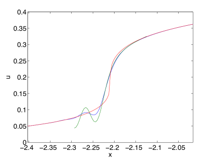
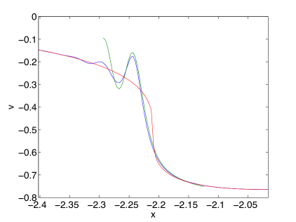
Refer to caption
Refer to caption
Figure 2: Solution to the defocusing cubic NLS equation for the initial data ψ0(x)=sech xsubscript𝜓0𝑥sech 𝑥\psi_{0}(x)=\mbox{sech }x and ϵ=0.01italic-ϵ0.01\epsilon=0.01 at the critical time t0subscript𝑡0t_{0} in blue, the corresponding semiclassical solution in red and the P2Isuperscriptsubscriptabsent𝐼2{}_{I}^{2} solution (3.5) in green; on the left the function u𝑢u, on the right the function v𝑣v.

The corresponding Riemann invariants can be seen in Fig. 3.
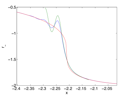
Refer to caption
Refer to caption
Refer to caption
Refer to caption
Figure 3: Solution to the defocusing cubic NLS equation for the initial data ψ0(x)=sech xsubscript𝜓0𝑥sech 𝑥\psi_{0}(x)=\mbox{sech }x at the critical time t0subscript𝑡0t_{0} in blue, the corresponding semiclassical solution in red and the P2Isuperscriptsubscriptabsent𝐼2{}_{I}^{2} solution (3.5) in green; on the left the Riemann invariant rsubscript𝑟r_{-}, on the right the invariant r+subscript𝑟r_{+}. The upper figures are for ϵ=0.01italic-ϵ0.01\epsilon=0.01, the lower ones for ϵ=0.001italic-ϵ0.001\epsilon=0.001.

For smaller ϵitalic-ϵ\epsilon the agreement of NLS and semiclassical solution becomes better. We show the Riemann invariants r±subscript𝑟plus-or-minusr_{\pm} for ϵ=103italic-ϵsuperscript103\epsilon=10^{-3} in Fig. 3. Notice that there are also oscillations in the invariant r+subscript𝑟r_{+} which stays smooth at this point in the semiclassical limit.

8.2 sechx𝑥\,x initial data for the defocusing quintic NLS equation

We will first study the initial data ψ0(x)=sech xsubscript𝜓0𝑥sech 𝑥\psi_{0}(x)=\mbox{sech }x for values of ϵitalic-ϵ\epsilon of 0.10.10.1, 0.090.090.09,…, 0.010.010.01, 0.0090.0090.009,…, 0.0010.0010.001. In this case there are two break-up points at ±xcplus-or-minussubscript𝑥𝑐\pm x_{c} with xc=ln((3+1)/2)+3/2)1.5245x_{c}=\ln((\sqrt{3}+1)/\sqrt{2})+\sqrt{3}/2)\sim 1.5245 at the same time t0=33/41.2990subscript𝑡0334similar-to1.2990t_{0}=3\sqrt{3}/4\sim 1.2990. The solution up to the critical time can be seen in Fig. 4, where the defocusing effect of the equation can be recognized. The critical value of the Riemann invariants at the respective break-up point is ±2/3plus-or-minus23\pm 2/3. We will consider in the following always the break-up for negative values of x𝑥x where the Riemann invariant r=vusubscript𝑟𝑣𝑢r_{-}=v-u has a gradient catastrophe.

Refer to caption
Figure 4: Solution to the defocusing quintic NLS equation for the initial data ψ0(x)=sech xsubscript𝜓0𝑥sech 𝑥\psi_{0}(x)=\mbox{sech }x and ϵ=0.01italic-ϵ0.01\epsilon=0.01. The critical time is t01.2990similar-tosubscript𝑡01.2990t_{0}\sim 1.2990.

At the critical time the difference of the Riemann invariants rsubscript𝑟r_{-} between the semiclassical solution and the solution to the focusing quintic NLS scales roughly as ϵ2/7superscriptitalic-ϵ27\epsilon^{2/7}. More precisely we find via a linear regression analysis for the logarithm of the difference ΔsubscriptΔ\Delta_{-} between NLS and semiclassical solution a scaling of the form Δϵaproportional-toΔsuperscriptitalic-ϵ𝑎\Delta\propto\epsilon^{a} with a=0.2952𝑎0.2952a=0.2952 (2/70.2857similar-to270.28572/7\sim 0.2857) with standard deviation σa=0.0017subscript𝜎𝑎0.0017\sigma_{a}=0.0017 and correlation coefficient r=0.9999𝑟0.9999r=0.9999. At the same point the difference Δ+subscriptΔ\Delta_{+} between the Riemann invariants r+=v+usubscript𝑟𝑣𝑢r_{+}=v+u between the semiclassical and the NLS solution scales roughly as ϵ4/7superscriptitalic-ϵ47\epsilon^{4/7} as predicted by the theory. A linear regression analysis for the logarithm of the difference Δ+subscriptΔ\Delta_{+} gives a scaling of the form Δϵaproportional-toΔsuperscriptitalic-ϵ𝑎\Delta\propto\epsilon^{a} with a=0.5988𝑎0.5988a=0.5988 (4/70.5714similar-to470.57144/7\sim 0.5714) with standard deviation σa=0.0053subscript𝜎𝑎0.0053\sigma_{a}=0.0053 and correlation coefficient r=0.9998𝑟0.9998r=0.9998.

In Fig. 5, the NLS solution, the semiclassical solution and the P2Isuperscriptsubscriptabsent𝐼2{}_{I}^{2} solution (3.5) can be seen at the critical time close to the critical point of the semiclassical solution.
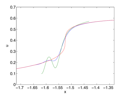
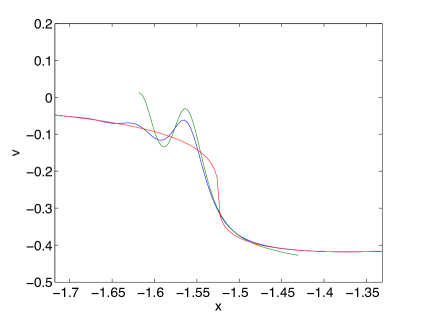
Refer to caption
Refer to caption
Figure 5: Solution to the defocusing quintic NLS equation for the initial data ψ0(x)=sech xsubscript𝜓0𝑥sech 𝑥\psi_{0}(x)=\mbox{sech }\,x and ϵ=0.01italic-ϵ0.01\epsilon=0.01 at the critical time t0subscript𝑡0t_{0} in blue, the corresponding semiclassical solution in red and the P2Isuperscriptsubscriptabsent𝐼2{}_{I}^{2} solution (3.5) in green; on the left the function u𝑢u, on the right the function v𝑣v.

The corresponding Riemann invariants can be seen in Fig. 6.
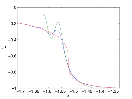
Refer to caption
Refer to caption
Refer to caption
Refer to caption
Figure 6: Solution to the defocusing quintic NLS equation for the initial data ψ0(x)=sech xsubscript𝜓0𝑥sech 𝑥\psi_{0}(x)=\mbox{sech }x at the critical time t0subscript𝑡0t_{0} in blue, the corresponding semiclassical solution in red and the P2Isuperscriptsubscriptabsent𝐼2{}_{I}^{2} solution (3.5) in green; on the left the Riemann invariant rsubscript𝑟r_{-}, on the right the invariant r+subscript𝑟r_{+}. The upper figures are for ϵ=0.01italic-ϵ0.01\epsilon=0.01, the lower ones for ϵ=0.001italic-ϵ0.001\epsilon=0.001.

For smaller ϵitalic-ϵ\epsilon the agreement of NLS and semiclassical solution becomes better. We show the Riemann invariants r±subscript𝑟plus-or-minusr_{\pm} for ϵ=103italic-ϵsuperscript103\epsilon=10^{-3} in Fig. 6. Note that there are also oscillations in the invariant rsubscript𝑟r_{-} which stays smooth at this point in the semiclassical limit.

The P2Isuperscriptsubscriptabsent𝐼2{}_{I}^{2} solution (3.5) gives a much better agreement with the NLS solution close to the critical point as can be seen in Fig. 5 and 6. The agreement is in fact so good that the difference of the solutions has to be studied. The P2Isuperscriptsubscriptabsent𝐼2{}_{I}^{2} solution only gives locally an asymptotic description, at larger distances from the critical point the semiclassical solution provides a better description as can be also seen from Fig. 7.
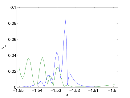
Refer to caption
Refer to caption
Figure 7: The modulus of the difference af the Riemann invariants for the defocusing quintic NLS equation for the initial data ψ0(x)=sech xsubscript𝜓0𝑥sech 𝑥\psi_{0}(x)=\mbox{sech }x for ϵ=0.01italic-ϵ0.01\epsilon=0.01 at the critical time t0subscript𝑡0t_{0} and the semiclassical solution in blue, and the difference between the corresponding P2Isuperscriptsubscriptabsent𝐼2{}_{I}^{2} solution (3.5) and the NLS solution in green; on the left the invariant that has a break-up in the semiclassical limit, on the right the invariant that stays smooth.

We can identify the regions where each of the asymptotic solutions gives a better description of NLS than the other by identifying the values xl,xrsubscript𝑥𝑙subscript𝑥𝑟x_{l},x_{r} such that for all xl<x<xrsubscript𝑥𝑙𝑥subscript𝑥𝑟x_{l}<x<x_{r} the P2Isuperscriptsubscriptabsent𝐼2{}_{I}^{2} solution provides a better asymptotic description than the semiclassical solution. Due to the oscillatory character of the NLS and the P2Isuperscriptsubscriptabsent𝐼2{}_{I}^{2} solution (3.5), such a definition leads to ambiguities and oscillations also in the boundaries of these zones for r±subscript𝑟plus-or-minusr_{\pm}. No clear scaling could thus be identified for these limits. The oscillatory character of the solution also implies there is no obvious scaling of the maximal error in the asymptotic description for the values of ϵitalic-ϵ\epsilon we could treat.

The matching procedure nonetheless clearly improves the asymptotic description near the critical point. In Fig. 8 we see the difference between this matched asymptotic solution and the NLS solution for two values of ϵitalic-ϵ\epsilon. Visibly the zone, where the solutions are matched, decreases with ϵitalic-ϵ\epsilon (note the rescaling of the x𝑥x-axes with a factor ϵ6/7superscriptitalic-ϵ67\epsilon^{6/7}).

Refer to caption
Refer to caption
Figure 8: In the upper part of the left figure one can see the modulus of the difference ΔsubscriptΔ\Delta_{-} of the Riemann invariant for the defocusing quintic NLS equation for the initial data ψ0(x)=sech xsubscript𝜓0𝑥sech 𝑥\psi_{0}(x)=\mbox{sech }x at the critical time t0subscript𝑡0t_{0} and the semiclassical solution for ϵ=0.01italic-ϵ0.01\epsilon=0.01. The lower part shows the same difference, which is replaced close to the critical point by the difference between NLS solution and the P2Isuperscriptsubscriptabsent𝐼2{}_{I}^{2} solution (3.5) (in red where the error is smaller than the one shown above). The right figure shows the same situation as the lower figure on the left for ϵ=0.01italic-ϵ0.01\epsilon=0.01 above and ϵ=0.001italic-ϵ0.001\epsilon=0.001 below. The x𝑥x-axes are rescaled by a factor ϵ6/7superscriptitalic-ϵ67\epsilon^{6/7}.

The same procedure can be carried out for the invariant r+subscript𝑟r_{+} which stays smooth at this point. Obviously the P2Isuperscriptsubscriptabsent𝐼2{}_{I}^{2} solution (3.5) provides a description of higher order at this point as can be seen in Fig. 9. Thus the P2Isuperscriptsubscriptabsent𝐼2{}_{I}^{2} solution (3.5) provides as expected an asymptotic description of the oscillations for the Riemann invariant which remains smooth in the semiclassical limit.
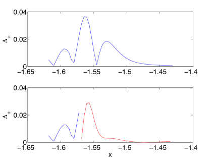
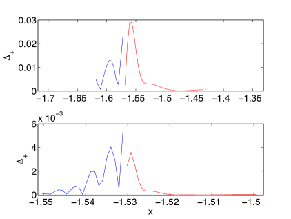
Refer to caption
Refer to caption
Figure 9: In the upper part of the left figure one can see the modulus of the difference Δ+subscriptΔ\Delta_{+} of the Riemann invariant for the defocusing quintic NLS equation for the initial data ψ0(x)=sech xsubscript𝜓0𝑥sech 𝑥\psi_{0}(x)=\mbox{sech }x at the critical time t0subscript𝑡0t_{0} and the semiclassical solution for ϵ=0.01italic-ϵ0.01\epsilon=0.01. The lower part shows the same difference, which is replaced close to the critical point by the difference between NLS solution and the P2Isuperscriptsubscriptabsent𝐼2{}_{I}^{2} solution (3.5) (in red where the error is smaller than the one shown above). The right figure shows the same situation as the lower figure on the left for ϵ=0.01italic-ϵ0.01\epsilon=0.01 above and ϵ=0.001italic-ϵ0.001\epsilon=0.001 below. The x𝑥x-axes are rescaled by a factor ϵ6/7superscriptitalic-ϵ67\epsilon^{6/7}.

The P2Isuperscriptsubscriptabsent𝐼2{}_{I}^{2} solution (3.5) holds for small |xxc|𝑥subscript𝑥𝑐|x-x_{c}| and |tt0|𝑡subscript𝑡0|t-t_{0}|. To illustrate the latter effect, we compare it with the NLS solution for the times t±=t0±0.0027subscript𝑡plus-or-minusplus-or-minussubscript𝑡00.0027t_{\pm}=t_{0}\pm 0.0027. Note that tt0𝑡subscript𝑡0t-t_{0} appears in the formula (3.5) for the P2Isuperscriptsubscriptabsent𝐼2{}_{I}^{2} solution at several places with different powers of ϵitalic-ϵ\epsilon. Thus in contrast to the elliptic case (5.23), there is no simple dependence on t𝑡t in the hyperbolic case. In Fig. 10 we show the quantities r±subscript𝑟plus-or-minusr_{\pm} at the time t±subscript𝑡plus-or-minust_{\pm}. It can be seen that the P2Isuperscriptsubscriptabsent𝐼2{}_{I}^{2} solution gives again a clearly better asymptotic description near the break-up point than the semiclassical solution.
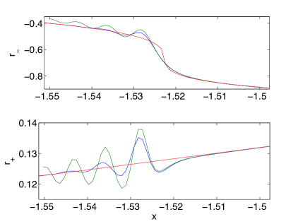
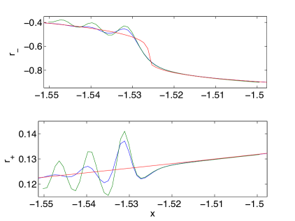
Refer to caption
Refer to caption
Figure 10: Solution to the defocusing quintic NLS equation for the initial data ψ0(x)=sech xsubscript𝜓0𝑥sech 𝑥\psi_{0}(x)=\mbox{sech }x and ϵ=0.01italic-ϵ0.01\epsilon=0.01 in blue, the corresponding semiclassical solution in red and the P2Isuperscriptsubscriptabsent𝐼2{}_{I}^{2} solution (3.5) in green; above the function rsubscript𝑟r_{-}, below the function r+subscript𝑟r_{+}. On the left at the time t=t00.0027subscript𝑡subscript𝑡00.0027t_{-}=t_{0}-0.0027 on the right at the time t+=t0+0.0027subscript𝑡subscript𝑡00.0027t_{+}=t_{0}+0.0027

8.3 ‘Dark’ initial data for the defocusing quintic NLS

It is well known that the defocusing cubic NLS equation has exact solutions called dark solitons, i.e., solutions that do not tend to zero for |x|𝑥|x|\to\infty. Such solutions are physically problematic since they have infinite energy and are mathematically difficult to handle, but they are nonetheless of importance in applications. Therefore we will here also study initial data which do not decay to zero at spatial infinity. We will consider the example ψ0(x)=tanh2xsubscript𝜓0𝑥superscript2𝑥\psi_{0}(x)=\tanh^{2}x in the following. The time evolution of the solution up to the critical time t01.3448similar-tosubscript𝑡01.3448t_{0}\sim 1.3448 can be seen in Fig. 11. The steepening of the two fronts of the pulse can be seen as well as the formation of a small oscillation on each side. For times tt0much-greater-than𝑡subscript𝑡0t\gg t_{0}, each of the initial oscillations develops into an oscillatory zone which will eventually overlap.
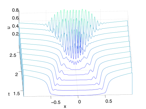
Refer to caption
Figure 11: Solution to the defocusing quintic NLS equation for the initial data ψ0(x)=tanh2xsubscript𝜓0𝑥superscript2𝑥\psi_{0}(x)=\tanh^{2}x and ϵ=0.01italic-ϵ0.01\epsilon=0.01. The critical time is t01.3448similar-tosubscript𝑡01.3448t_{0}\sim 1.3448.

Clearly there will be two regions with strong gradients symmetric in x𝑥x. We will concentrate on positive values of x𝑥x where the Rieman invariant rsubscript𝑟r_{-} breaks in the semiclassical solution. In Fig. 12 the Riemann invariants for the NLS solution, the corresponding semiclassical solution and the P2Isuperscriptsubscriptabsent𝐼2{}_{I}^{2} asymptotics (3.5) can be seen close to xc0.5476similar-tosubscript𝑥𝑐0.5476x_{c}\sim 0.5476 for ϵ=0.001italic-ϵ0.001\epsilon=0.001.

Refer to caption
Refer to caption
Figure 12: Solution to the defocusing quintic NLS equation for the initial data ψ0(x)=tanh2xsubscript𝜓0𝑥superscript2𝑥\psi_{0}(x)=\tanh^{2}x and ϵ=0.001italic-ϵ0.001\epsilon=0.001 at the critical time t0subscript𝑡0t_{0} in blue, the corresponding semiclassical solution in red and the P2Isuperscriptsubscriptabsent𝐼2{}_{I}^{2} solution (3.5) in green; on the left the Riemann invariant rsubscript𝑟r_{-}, on the right the invariant r+subscript𝑟r_{+}.

8.4 Defocusing nonlocal NLS

We will study the small dispersion limit of the nonlocal NLS (5.6) close to the break-up of the corresponding semiclassical solutions. We will concentrate on values of η𝜂\eta such that ηϵ21much-less-than𝜂superscriptitalic-ϵ21\eta\epsilon^{2}\ll 1 for all studied values of ϵitalic-ϵ\epsilon. For both cases we will consider the initial data ψ0=sech xsubscript𝜓0sech 𝑥\psi_{0}=\mbox{sech }x. In the defocusing variant of the nonlocal NLS equation (5.6), the nonlocality has the effect to reduce the defocusing effect of the equation. The dispersion and the steepening of the gradient close to the break-up of the corresponding semiclassical solution is reduced as can be seen in Fig. 13. This also suppresses the formation of dispersive shocks, i.e., the oscillations close to the gradient catastrophe of the semiclassical solution (see [57]). Due to the possible sign change of the quantity ρ𝜌\rho in (3.26), an other effect can be observed in Fig. 13: for large enough η𝜂\eta, the oscillations appear on the other side of the critical point. We again consider the initial data ψ0=sech xsubscript𝜓0sech 𝑥\psi_{0}=\mbox{sech }x at the critical time t01.5244similar-tosubscript𝑡01.5244t_{0}\sim 1.5244 near the break-up of the Riemann invariant rsubscript𝑟r_{-} at xc2.2094similar-tosubscript𝑥𝑐2.2094x_{c}\sim-2.2094 in the semiclassical limit.

Refer to caption
Figure 13: Solution to the defocusing nonlocal NLS equation (5.6) for the initial data ψ0(x)=sech xsubscript𝜓0𝑥sech 𝑥\psi_{0}(x)=\mbox{sech }x and ϵ=0.01italic-ϵ0.01\epsilon=0.01 at the time t0=1.5244t_{0}=\sim 1.5244 for two values of η𝜂\eta.

For larger times this implies for ρ<0𝜌0\rho<0 that there is just one oscillation to the right of xcsubscript𝑥𝑐-x_{c} as described asymptotically by the P2Isuperscriptsubscriptabsent𝐼2{}_{I}^{2} solution, and many small oscillations on the other side of the critical point as can be seen in Fig. 14. The situation is similar to the one of certain Kawahara solutions in the small dipsersion limit as discussed in [47].
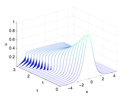
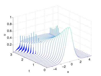
Refer to caption
Refer to caption
Figure 14: Solution to the defocusing nonlocal NLS equation (5.6) for the initial data ψ0(x)=sech xsubscript𝜓0𝑥sech 𝑥\psi_{0}(x)=\mbox{sech }x and ϵ=0.01italic-ϵ0.01\epsilon=0.01; for η=1𝜂1\eta=1 on the left, for η=100𝜂100\eta=100 on the right. The critical time is t01.5244similar-tosubscript𝑡01.5244t_{0}\sim 1.5244.

In the case ρ=0𝜌0\rho=0 in (3.26) the P2Isuperscriptsubscriptabsent𝐼2{}_{I}^{2} asymptotics cannot be used. In the present example this is the case for η1.3060similar-to𝜂1.3060\eta\sim 1.3060. The solution at the critical time for this value of η𝜂\eta can be seen in Fig. 15.

Refer to caption
Figure 15: Solution to the defocusing nonlocal NLS equation (5.6) for the initial data ψ0(x)=sech xsubscript𝜓0𝑥sech 𝑥\psi_{0}(x)=\mbox{sech }x, ϵ=0.1italic-ϵ0.1\epsilon=0.1 and the non-generic value η1.3060similar-to𝜂1.3060\eta\sim 1.3060 at the critical time t01.5244similar-tosubscript𝑡01.5244t_{0}\sim 1.5244.

For smaller η𝜂\eta, the nonlocal NLS behaves qualitatively like the defocusing cubic NLS close to the critical time as can be seen in Fig. 16 for the Riemann invariant breaking in the semiclassical limit. For smaller values of ϵitalic-ϵ\epsilon the same behavior can be seen, but on smaller scales. Again there are two different scales in the P2Isuperscriptsubscriptabsent𝐼2{}_{I}^{2} asymptotics (3.5) which means there is no clear scaling in the coordinates x𝑥x and t𝑡t. For the representation, we nonetheless rescale x𝑥x by a factor of ϵ6/7superscriptitalic-ϵ67\epsilon^{6/7} to be able to compare the case ϵ=0.001italic-ϵ0.001\epsilon=0.001 with ϵ=0.01italic-ϵ0.01\epsilon=0.01. The y𝑦y-axes are rescaled to optimally use the space of the figure. The approximation visibly gets better with smaller ϵitalic-ϵ\epsilon. The Riemann invariant staying smooth in the semiclassical limit can be seen for the same situation in the right part of Fig. 16. The asymptotic description again improves clearly with smaller ϵitalic-ϵ\epsilon.

Refer to caption
Refer to caption
Figure 16: Riemann invariant rsubscript𝑟r_{-} on the left and r+subscript𝑟r_{+} on the right of the solution to the defocusing nonlocal NLS equation (5.6) for the initial data ψ0(x)=sech xsubscript𝜓0𝑥sech 𝑥\psi_{0}(x)=\mbox{sech }x and η=1𝜂1\eta=1 at the time t01.5244similar-tosubscript𝑡01.5244t_{0}\sim 1.5244 for two values of ϵitalic-ϵ\epsilon in blue, the corresponding semiclassical solution in red and the P12 solution (3.5) in green.

For larger η𝜂\eta the smoothing out of the gradients near the shock of the semiclassical equations implies that the semiclassical solution only provides a valid asymptotic description for larger |xxc|𝑥subscript𝑥𝑐|x-x_{c}| than is the case for smaller η𝜂\eta. The P2Isuperscriptsubscriptabsent𝐼2{}_{I}^{2} asymptotics (3.5) catches this behavior as can be seen for η=100𝜂100\eta=100 in Fig. 17 on the left for the invariant breaking in the semiclassical limit. There are essentially no oscillations in this case.
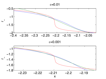
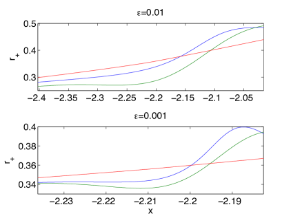
Refer to caption
Refer to caption
Figure 17: Riemann invariant rsubscript𝑟r_{-} on the left and Riemann invariant r+subscript𝑟r_{+} on the right for the solution to the defocusing nonlocal NLS equation (5.6) for the initial data ψ0(x)=sech xsubscript𝜓0𝑥sech 𝑥\psi_{0}(x)=\mbox{sech }x and η=100𝜂100\eta=100 at the time t01.5244similar-tosubscript𝑡01.5244t_{0}\sim 1.5244 for two values of ϵitalic-ϵ\epsilon in blue, the corresponding semiclassical solution in red and the P2Isuperscriptsubscriptabsent𝐼2{}_{I}^{2} solution (3.5) in green.

The invariant r+subscript𝑟r_{+} can be seen on the right part of Fig. 17. There is essentially only one oscillation to the right of the critical point in this case. The P2Isuperscriptsubscriptabsent𝐼2{}_{I}^{2} asymptotics has an oscillation close to the oscillation of the nonlocal NLS and thus catches this behavior in an asymptotic sense.

9 Numerical study of focusing generalized and nonlocal NLS equations

In this section we will study numerically solutions to the focusing NLS before and close to the break up of the corresponding semiclassical solutions. Since the case of the focusing cubic NLS was studied in detail in [46], we concentrate here on the not integrable quintic NLS. We compare solutions to NLS and semiclassical equations and for tt0similar-to𝑡subscript𝑡0t\sim t_{0} to an asymptotic solution in terms of the tritronquée solution of the Painlevé-I equation. The same is done for a nonlocal variant of the cubic NLS equation.

9.1 sechx𝑥\,x initial data for the focusing quintic NLS

We will first study the initial data ψ0(x)=sech xsubscript𝜓0𝑥sech 𝑥\psi_{0}(x)=\mbox{sech }x for several values of ϵitalic-ϵ\epsilon, i.e., ϵ=0.1italic-ϵ0.1\epsilon=0.1, 0.090.090.09,…,0.010.010.01. For this example, the break-up occurs for the semiclassical solution at t0=0.4119subscript𝑡00.4119t_{0}=0.4119\ldots at xc=0subscript𝑥𝑐0x_{c}=0 with the critical values uc=1.5858subscript𝑢𝑐1.5858u_{c}=1.5858\ldots and vc=0subscript𝑣𝑐0v_{c}=0. The solution up to the critical time can be seen in Fig. 18. The focusing effect can be clearly recognized.
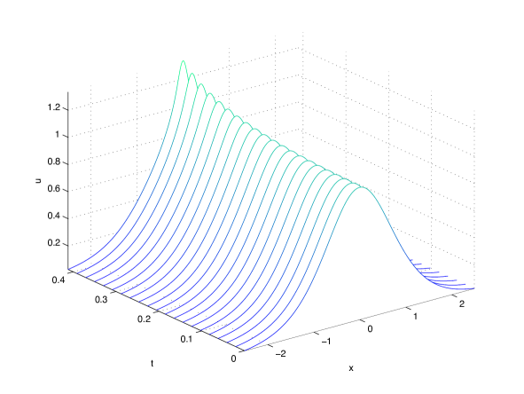
Refer to caption
Figure 18: Solution to the focusing quintic NLS equation for the initial data ψ0(x)=sech xsubscript𝜓0𝑥sech 𝑥\psi_{0}(x)=\mbox{sech }x and ϵ=0.1italic-ϵ0.1\epsilon=0.1 up to the critical time t0subscript𝑡0t_{0} in blue.

For times much smaller than the critical time one finds that the difference between semiclassical and NLS solution scales as ϵ2superscriptitalic-ϵ2\epsilon^{2}. For instance for t=t0/2t0𝑡subscript𝑡02much-less-thansubscript𝑡0t=t_{0}/2\ll t_{0} we obtain for Δ=|uNLSusc|Δsubscript𝑢𝑁𝐿𝑆subscript𝑢𝑠𝑐\Delta=|u_{NLS}-u_{sc}| via a linear regression analysis for the logarithm of ΔΔ\Delta a scaling of the form Δϵaproportional-toΔsuperscriptitalic-ϵ𝑎\Delta\propto\epsilon^{a} with a=1.985𝑎1.985a=1.985 with standard deviation σa=0.0018subscript𝜎𝑎0.0018\sigma_{a}=0.0018 and correlation coefficient r=0.999998𝑟0.999998r=0.999998.
At the critical time the difference between the semiclassical solution and the solution to the focusing quintic NLS scales roughly as ϵ2/5superscriptitalic-ϵ25\epsilon^{2/5}. More precisely we find via a linear regression analysis for the logarithm of the difference ΔΔ\Delta between NLS and semiclassical solution a scaling of the form Δϵaproportional-toΔsuperscriptitalic-ϵ𝑎\Delta\propto\epsilon^{a} with a=0.403𝑎0.403a=0.403 with standard deviation σa=0.001subscript𝜎𝑎0.001\sigma_{a}=0.001 and correlation coefficient r=0.99998𝑟0.99998r=0.99998. As can be seen in Fig. 19, the semiclassical solution has a cusp. Thus the maximal difference between semiclassical and NLS solution is always observed for the critical point.
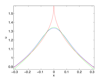
Refer to caption
Refer to caption
Refer to caption
Refer to caption
Figure 19: Solution to the focusing quintic NLS equation for the initial data ψ0(x)=sech xsubscript𝜓0𝑥sech 𝑥\psi_{0}(x)=\mbox{sech }x at the critical time t0subscript𝑡0t_{0} in blue, the corresponding semiclassical solution in red and the PI solution (5.23) in green; on the left the function u𝑢u, on the right the function v𝑣v. For the upper two figures we have ϵ=0.1italic-ϵ0.1\epsilon=0.1, for the lower ones ϵ=0.01italic-ϵ0.01\epsilon=0.01.

The x𝑥x-axis of the figures in the lower row is rescaled by factor ϵ4/5superscriptitalic-ϵ45\epsilon^{4/5} with respect to the figures in the upper row.

For smaller ϵitalic-ϵ\epsilon the agreement of NLS and semiclassical solution becomes better, but the biggest difference is always at the critical point as can be seen in the bottom of Fig. 19.

The PI solution (5.23) gives a much better agreement with the NLS solution close to the critical point as can be seen in Fig. 19. The agreement is in fact so good that the difference of the solutions has to be studied. The PI solution only gives locally an asymptotic description, at larger distances from the critical point the semiclassical solution provides a better description as can be also seen from Fig. 20.
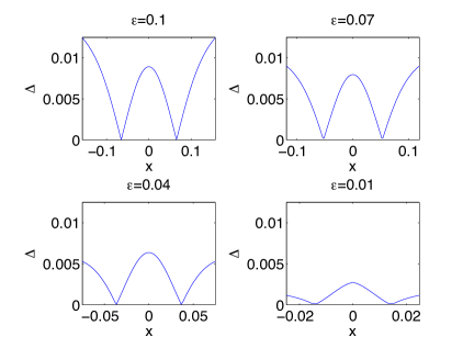
Refer to caption
Refer to caption
Figure 20: The modulus of the difference of the solution to the focusing quintic NLS equation for the initial data ψ0(x)=sech xsubscript𝜓0𝑥sech 𝑥\psi_{0}(x)=\mbox{sech }x for ϵ=0.1italic-ϵ0.1\epsilon=0.1 at the critical time t0subscript𝑡0t_{0} and the difference between the corresponding PI solution (5.23) for several values of ϵitalic-ϵ\epsilon; on the left the difference ΔΔ\Delta for u𝑢u, on the right the difference ΔvsubscriptΔ𝑣\Delta_{v} for v𝑣v. The x𝑥x-axes are rescaled with a factor ϵ4/5superscriptitalic-ϵ45\epsilon^{4/5}.

We can identify the regions where each of the asymptotic solutions gives a better description of NLS than the other by identifying the value of xrsubscript𝑥𝑟x_{r} such that for all x>xr𝑥subscript𝑥𝑟x>x_{r} the semiclassical solutions gives a better asymptotic description than the multiscales solution (since the solution is symmetric with respect to x𝑥x, we only consider positive values of x𝑥x here). We find that the width of this zone scales roughly as ϵ3/5superscriptitalic-ϵ35\epsilon^{3/5}. A linear regression analysis for the dependence of log10xrsubscript10subscript𝑥𝑟\log_{10}x_{r} on log10ϵsubscript10italic-ϵ\log_{10}\epsilon yields a=0.634𝑎0.634a=0.634 with standard deviation σa=0.0036subscript𝜎𝑎0.0036\sigma_{a}=0.0036 and correlation coefficient r=0.99993𝑟0.99993r=0.99993.

This matching procedure clearly improves the NLS description near the critical point. In Fig. 21 we see the difference between this matched asymptotic solution and the NLS solution for two values of ϵitalic-ϵ\epsilon. Visibly the zone, where the solutions are matched, decreases with ϵitalic-ϵ\epsilon (note the rescaling of the x𝑥x-axes by a factor ϵ4/5superscriptitalic-ϵ45\epsilon^{4/5}).

Refer to caption
Refer to caption
Figure 21: In the upper part of the left figure one can see the modulus of the difference of the solution u𝑢u to the focusing quintic NLS equation for the initial data ψ0(x)=sech xsubscript𝜓0𝑥sech 𝑥\psi_{0}(x)=\mbox{sech }x at the critical time t0subscript𝑡0t_{0} and the semiclassical solution for ϵ=0.1italic-ϵ0.1\epsilon=0.1. The lower part shows the same difference, which is replaced close to the critical point by the difference between NLS solution and the PI solution (5.23) (in red where the error is smaller than the one shown above). The right figure shows the same situation as the lower figure on the left for ϵ=0.1italic-ϵ0.1\epsilon=0.1 above and ϵ=0.01italic-ϵ0.01\epsilon=0.01 below. The x𝑥x-axes are rescaled in this figure by a factor ϵ4/5superscriptitalic-ϵ45\epsilon^{4/5}.

A linear regression analysis for the logarithm of the difference ΔΔ\Delta between NLS and multiscales solution in the matching zone gives a scaling of the form Δϵaproportional-toΔsuperscriptitalic-ϵ𝑎\Delta\propto\epsilon^{a} with a=0.6659𝑎0.6659a=0.6659 with standard deviation σa=0.032subscript𝜎𝑎0.032\sigma_{a}=0.032 and correlation coefficient r=0.995𝑟0.995r=0.995. The found scaling is thus in the whole interval clearly better than the ϵ2/5superscriptitalic-ϵ25\epsilon^{2/5} of the semiclassical solution, but does not reach the expected ϵ4/5superscriptitalic-ϵ45\epsilon^{4/5} scaling in the whole interval. This indicates that transition formulae between the multiscales and the semiclassical solution have to be established as in [60] for KdV, which is, however, beyond the scope of the present paper.

The PI solution (5.23) holds for small |xxc|𝑥subscript𝑥𝑐|x-x_{c}| and |tt0|𝑡subscript𝑡0|t-t_{0}|. To illustrate the latter effect, we compare it with the NLS solution for the times t±(ϵ)=t0±0.01ϵ4/5subscript𝑡plus-or-minusitalic-ϵplus-or-minussubscript𝑡00.01superscriptitalic-ϵ45t_{\pm}(\epsilon)=t_{0}\pm 0.01\epsilon^{4/5} where we take care of the scaling of t𝑡t in (4.26). In Fig. 22 we show the quantity ΔΔ\Delta for 2 values of ϵitalic-ϵ\epsilon at the times t(ϵ)subscript𝑡italic-ϵt_{-}(\epsilon). The x𝑥x-axes are rescaled by a factor ϵ4/5superscriptitalic-ϵ45\epsilon^{4/5}. It can be seen that the quality of the asymptotic description is slightly lower than at the critical time, but that the error is of a similar order. The situation is similar at the time t+=t0+0.01ϵ4/5subscript𝑡subscript𝑡00.01superscriptitalic-ϵ45t_{+}=t_{0}+0.01\epsilon^{4/5} as can be seen also in Fig. 22.

Refer to caption
Refer to caption
Figure 22: The modulus of the difference of the solution u𝑢u to the focusing quintic NLS equation for the initial data ψ0(x)=sech xsubscript𝜓0𝑥sech 𝑥\psi_{0}(x)=\mbox{sech }x for two values of ϵitalic-ϵ\epsilon at the time t(ϵ)=t00.01ϵ4/5subscript𝑡italic-ϵsubscript𝑡00.01superscriptitalic-ϵ45t_{-}(\epsilon)=t_{0}-0.01\epsilon^{4/5} on the left and at the time t+(ϵ)=t0+0.01ϵ4/5subscript𝑡italic-ϵsubscript𝑡00.01superscriptitalic-ϵ45t_{+}(\epsilon)=t_{0}+0.01\epsilon^{4/5} on the right, and the corresponding PI solution (5.23).

9.2 Non-symmetric initial data for the focusing quintic NLS

To study solutions to the focusing quintic NLS for the asymmetric initial data (6.4), we first have to solve equations (6.4) numerically. This is done for values of |x|<15𝑥15|x|<15 in a standard way by solving (6.4) on some Chebyshev collocation points with a Newton iteration. The choice of this interval is determined by the fact that the residual of the Newton iterate is smaller than 1010superscript101010^{-10} on the whole intervall. We choose Nc=512subscript𝑁𝑐512N_{c}=512 collocation points to ensure that the coefficients of an expansion of the solution decrease to machine precision and that the solution is thus numerically fully resolved. For values of |x|>15𝑥15|x|>15, we solve (6.4) asymptotically,

r=1+(2i)12αexp(x)+(2i)24αexp(2x)(0.5+2α2ln(2i)+α+αx)+𝒪(exp(3x))𝑟1superscript2𝑖12𝛼𝑥superscript2𝑖24𝛼2𝑥0.52superscript𝛼22𝑖𝛼𝛼𝑥𝒪3𝑥r=-1+(2i)^{1-2\alpha}\exp(-x)+(2i)^{2-4\alpha}\exp(-2x)(-0.5+2\alpha^{2}\ln(2i)+\alpha+\alpha x)+\mathcal{O}(\exp(-3x)) (9.1)

for x+𝑥x\to+\infty and

r=1+iexp(x)21+2α+22+4αexp(2x)(0.5+2α2ln(2)+αxα)+𝒪(exp(3x))𝑟1𝑖𝑥superscript212𝛼superscript224𝛼2𝑥0.52superscript𝛼22𝛼𝑥𝛼𝒪3𝑥r=1+i\exp(x)2^{1+2\alpha}+2^{2+4\alpha}\exp(2x)(-0.5+2\alpha^{2}\ln(2)+\alpha x-\alpha)+\mathcal{O}(\exp(3x)) (9.2)

for x𝑥x\to-\infty. Machine precision is reached for |x|>15𝑥15|x|>15 for this asymptotic solution. Initial data for α=0.2𝛼0.2\alpha=0.2 can be seen in Fig. 23.

Refer to caption
Figure 23: Asymmetric initial data for the focusing quintic NLS equation according to (6.26) for α=0.2𝛼0.2\alpha=0.2.

To obtain initial data for the NLS equation from r=v+iu𝑟𝑣𝑖𝑢r=v+iu in the form ψ=uexp(ix0xv(x)𝑑x/ϵ)𝜓𝑢𝑖superscriptsubscriptsubscript𝑥0𝑥𝑣superscript𝑥differential-dsuperscript𝑥italic-ϵ\psi=\sqrt{u}\exp(i\int_{x_{0}}^{x}v(x^{\prime})dx^{\prime}/\epsilon), we have to integrate the real part of r𝑟r with respect to x𝑥x. This is done by using an expansion of the solution for |x|<15𝑥15|x|<15 in terms of Chebyshev polynomials via a discrete cosine transform (this is the reason why the solution was computed on Chebyshev collocation points) and applying the well known formula for the integral of Chebyshev polynomials. For values of |x|>15𝑥15|x|>15, the asymptotic formulae (9.1) and (9.2) are integrated analytically by choosing the integration constants to obtain a continuous matching with the numerically integrated v𝑣v. This way we obtain initial data with an accuracy of better than 1010superscript101010^{-10}. We put the Krasny filter to the order of this treshold and thus obtain initial data resolved up to the level of the Krasny filter.

For ϵ=0.1italic-ϵ0.1\epsilon=0.1 the solution to the focusing quintic NLS equation for the asymmetric initial data as well as the semiclassical and the PI asymptotics (5.23) can be seen in Fig. 24. As expected the PI asymptotics gives a much better description of the NLS solution close to the critical point of the semiclassical solution. The error in the approximation is, however, also not symmetric here.
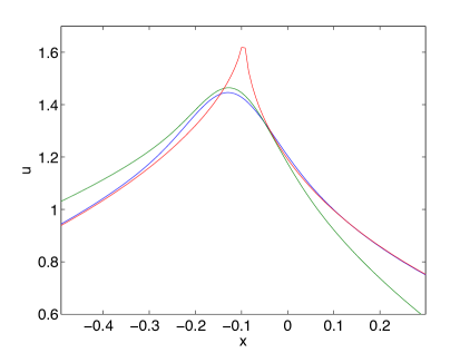
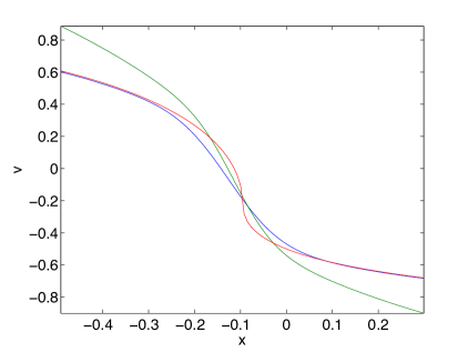
Refer to caption
Refer to caption
Refer to caption
Refer to caption
Figure 24: Solution to the focusing quintic NLS for the asymmetric initial data as in (6.26) for t=0𝑡0t=0 at the critical time in blue, the corresponding semiclassical solution in red and the PI asymptotics (5.23) in green; on the left the function u𝑢u, on the right the function v𝑣v. The upper figures are for ϵ=0.1italic-ϵ0.1\epsilon=0.1, the lower ones for ϵ=0.02italic-ϵ0.02\epsilon=0.02.

The agreement gets even better for smaller ϵitalic-ϵ\epsilon. We can reach values as low as ϵ=0.02italic-ϵ0.02\epsilon=0.02. For smaller ϵitalic-ϵ\epsilon, the blow-up singularity of quintic NLS solutions (see below) seems to be too close to the critical time of the semiclassical solution which breaks the code. The case ϵ=0.02italic-ϵ0.02\epsilon=0.02 is, however, numerically fully resolved. As can be seen in the lower row of Fig. 24, the agreement is as expected. Note that also in this case the x𝑥x-axes of the bottom figures have been rescaled by a factor ϵ4/5superscriptitalic-ϵ45\epsilon^{4/5}.

9.3 ‘Dark’ initial data

Focusing NLS equations do not have dark solitons as exact solutions, i.e., solutions which tend asymptotically to a non-zero constant and which vanish for finite values of x𝑥x. But it is mathematically interesting to study how initial data of this form lead to a break-up of the semiclassical equations, and how the corresponding NLS solution behaves in the vicinity of the critical point. We consider here initial data of the form ψ0=tanh2xsubscript𝜓0superscript2𝑥\psi_{0}=\tanh^{2}x. The solution breaks here in the form of two cusps symmetric with respect to x=0𝑥0x=0. The critical time is at t0=0.9041subscript𝑡00.9041t_{0}=0.9041\ldots, the cusps form at xc=±1.8723subscript𝑥𝑐plus-or-minus1.8723x_{c}=\pm 1.8723\ldots. The corresponding solution can be seen in Fig. 25.
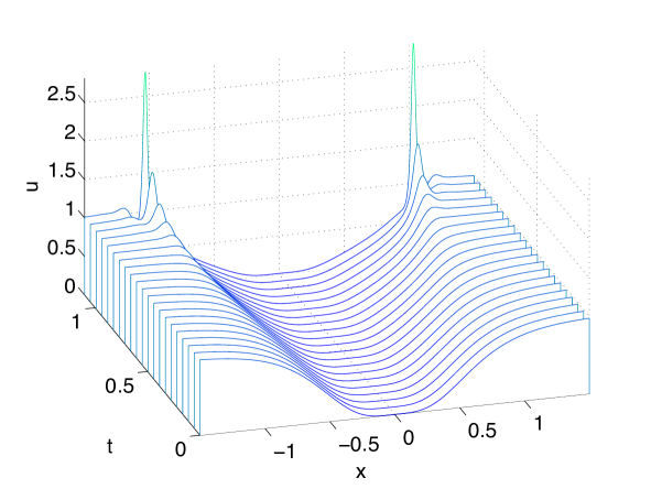
Refer to caption
Figure 25: Solution to the focusing quintic NLS equation for the dark initial data ψ0(x)=tanh2xsubscript𝜓0𝑥superscript2𝑥\psi_{0}(x)=\tanh^{2}x and ϵ=0.1italic-ϵ0.1\epsilon=0.1. The critical time is t0=0.9041subscript𝑡00.9041t_{0}=0.9041\ldots
Refer to caption
Refer to caption
Refer to caption
Refer to caption
Figure 26: Solution to the focusing quintic NLS for the dark initial data ψ0=tanh2xsubscript𝜓0superscript2𝑥\psi_{0}=\tanh^{2}x at the critical time in blue, the corresponding semiclassical solution in red and the PI asymptotics (5.23) in green; on the left the function u𝑢u, on the right the function v𝑣v. For the figures in the upper row ϵ=0.1italic-ϵ0.1\epsilon=0.1, for the ones in the lower row ϵ=0.04italic-ϵ0.04\epsilon=0.04.

For ϵ=0.1italic-ϵ0.1\epsilon=0.1 the solution to the focusing quintic NLS equation for the dark initial data as well as the semiclassical and the PI asymptotics (5.23) can be seen in Fig. 26. As expected the PI asymptotics gives a much better description of the NLS solution close to the critical point of the semiclassical solution. The agreement gets better for smaller ϵitalic-ϵ\epsilon. We can reach values as low as ϵ=0.04italic-ϵ0.04\epsilon=0.04, where the modulation instability leads to problems for smaller values of ϵitalic-ϵ\epsilon because of the asymptotically non-vanishing solution. The case ϵ=0.04italic-ϵ0.04\epsilon=0.04 is, however, numerically accessible. As can be seen in the bottom figures of Fig. 26, the agreement is as expected.

9.4 Blow-up

For the cubic focusing NLS, solutions in the semiclassical limit for times tt0much-greater-than𝑡subscript𝑡0t\gg t_{0} develop a zone of rapid modulated oscillations as can be seen for instance in Fig. 27. The central hump close to the critical time splits into several humps of smaller amplitude. For the quintic NLS on the other hand it is known, see e.g. [99], that initial data with negative energy have a blow-up in finite time. For the NLS with the semiclassical parameter ϵitalic-ϵ\epsilon we consider in this paper, this will be always the case for sufficiently small ϵitalic-ϵ\epsilon. Thus the solution of the quintic NLS looks for small ϵitalic-ϵ\epsilon very differently from the solution to the cubic NLS for the same initial data and the same value of ϵitalic-ϵ\epsilon as can be seen in Fig. 27. The central hump develops in this case into a blow-up.
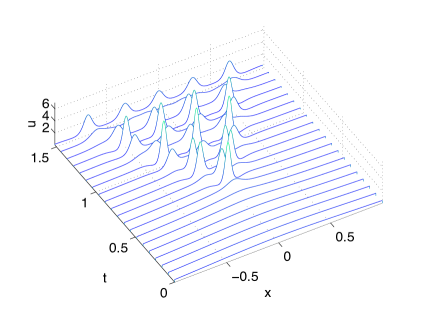
Refer to caption
Refer to caption
Figure 27: Solution to the focusing NLS equation for the initial data ψ0(x)=sech xsubscript𝜓0𝑥sech 𝑥\psi_{0}(x)=\mbox{sech }x and ϵ=0.1italic-ϵ0.1\epsilon=0.1; on the left the solution for the cubic NLS, on the right the solution to the quintic NLS.

For obvious reasons it is impossible to treat a blow-up exactly numerically, but the numerical solution can get sufficiently close to this case. Driscoll’s composite Runge-Kutta method produces an overflow error close to the Lsubscript𝐿L_{\infty} blow-up encountered here because of the term |ψ|4ψsuperscript𝜓4𝜓|\psi|^{4}\psi. We stop the code when this happens and note the last time with finite value of ψ𝜓\psi as a lower bound tBsubscript𝑡𝐵t_{B} for the blow-up time. The error in the determination of the blow-up time with this method is largest for larger ϵitalic-ϵ\epsilon. Using linear regression we find for ln(tBt0)=alnϵ+bsubscript𝑡𝐵subscript𝑡0𝑎italic-ϵ𝑏\ln(t_{B}-t_{0})=a\ln\epsilon+b for values of ϵ=0.01,0.02,,0.1italic-ϵ0.010.020.1\epsilon=0.01,0.02,\ldots,0.1 the value a=0.83𝑎0.83a=0.83 close to 4/5454/5 with standard deviation σa=0.0439subscript𝜎𝑎0.0439\sigma_{a}=0.0439, b=0.1267𝑏0.1267b=-0.1267 with standard deviation σb=0.0138subscript𝜎𝑏0.0138\sigma_{b}=0.0138 correlation coefficient r=0.999𝑟0.999r=0.999, see Fig. 28.

Refer to caption
Figure 28: The blow-up time as a function of ϵitalic-ϵ\epsilon for quintic NLS with sechxsech𝑥\mbox{sech}x initial data.

As expected from the PI solution (5.23), the time scales with ϵ4/5superscriptitalic-ϵ45\epsilon^{4/5}. Since we expect the error in the determination of the blow-up time to decrease with ϵitalic-ϵ\epsilon, a slightly stronger decrease with ϵitalic-ϵ\epsilon of the time tBsubscript𝑡𝐵t_{B} than predicted is no surprise.

It is an interesting question whether the blow-up time in the limit ϵ0italic-ϵ0\epsilon\to 0 is related to the first pole of the tritronquée solution on the negative real axis. In [73] it was shown that the first pole is located at

ξpole=2.3841687.subscript𝜉𝑝𝑜𝑙𝑒2.3841687\xi_{pole}=-2.3841687\ldots. (9.3)

Recalling formula (4.27) for the argument of the tritronquée solution in the approximation of the NLS solution near the point of elliptic umbilic catastrophe

ξ=i(u0V0(3V0+u0V0′′)2reiψ3ϵ4)15(xx0(v0+iu0V0)(tt0)).𝜉𝑖superscriptsubscript𝑢0superscriptsubscript𝑉0superscript3superscriptsubscript𝑉0subscript𝑢0subscriptsuperscript𝑉′′02𝑟superscript𝑒𝑖𝜓3superscriptitalic-ϵ415𝑥subscript𝑥0subscript𝑣0𝑖subscript𝑢0subscriptsuperscript𝑉0𝑡subscript𝑡0\xi=-i\left(\dfrac{u_{0}}{V_{0}^{\prime}}\left(3V_{0}^{\prime}+u_{0}V^{\prime\prime}_{0}\right)^{2}\dfrac{re^{i\psi}}{3\epsilon^{4}}\right)^{\frac{1}{5}}(x-x_{0}-(v_{0}+i\sqrt{u_{0}V^{\prime}_{0}})(t-t_{0})).

one can see that for quintic NLS and sechxsech𝑥\mbox{sech}x initial data, the point of elliptic umbilic catastrophe is at x0=0subscript𝑥00x_{0}=0, and for symmetry reasons, the blow up is at xB=0subscript𝑥𝐵0x_{B}=0. Using the above formula, with V(u)=u22𝑉𝑢superscript𝑢22V(u)=\frac{u^{2}}{2}, so that V0=u0subscriptsuperscript𝑉0subscript𝑢0V^{\prime}_{0}=u_{0}, V0′′=1superscriptsubscript𝑉0′′1V_{0}^{\prime\prime}=1 and

a+=ireiψ=i14(u0)23u02(u01)32.subscript𝑎𝑖𝑟superscript𝑒𝑖𝜓𝑖14superscriptsubscript𝑢023subscript𝑢02superscriptsubscript𝑢0132\;\;a_{+}=-\dfrac{i}{re^{i\psi}}=-i\dfrac{1}{4(u_{0})^{2}}\dfrac{3u_{0}-2}{(u_{0}-1)^{\frac{3}{2}}}.

with u0=1.5858u_{0}\simeq=1.5858 determined in (6.23) for this specific example, the blowup time tBsubscript𝑡𝐵t_{B} is then conjectured to satisfy the equation

ξpole2.38412.0324tBt0ϵ45.similar-to-or-equalssubscript𝜉𝑝𝑜𝑙𝑒2.3841similar-to-or-equals2.0324subscript𝑡𝐵subscript𝑡0superscriptitalic-ϵ45\xi_{pole}\simeq-2.3841\simeq-2.0324\dfrac{t_{B}-t_{0}}{\epsilon^{\frac{4}{5}}}.

which gives a value of |b|=ln(2.3841/2.0324)=0.1596𝑏2.38412.03240.1596|b|=\ln(2.3841/2.0324)=0.1596, in reasonable agreement with the numerically found value |b|0.1267similar-to𝑏0.1267|b|\sim 0.1267.

9.5 Focusing nonlocal NLS

We will study the small dispersion limit of the nonlocal NLS (5.6) close to the break-up of the corresponding semiclassical solutions. We will concentrate on values of η𝜂\eta such that ηϵ21much-less-than𝜂superscriptitalic-ϵ21\eta\epsilon^{2}\ll 1 for all studied values of ϵitalic-ϵ\epsilon. For both cases we will consider the initial data ψ0=sech xsubscript𝜓0sech 𝑥\psi_{0}=\mbox{sech }x. The effect of the nonlocality in (5.6) is to reduce the focusing effect of the focusing NLS. This means the larger η𝜂\eta, the smaller the value for the maximum at the critical time of the corresponding semiclassical solution, and the less pronounced the focusing of the maximum, i.e., smaller gradients in the solution. This effect can be clearly seen in Fig. 29.
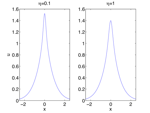
Refer to caption
Figure 29: Solution to the focusing nonlocal NLS equation (5.6) for the initial data ψ0(x)=sech xsubscript𝜓0𝑥sech 𝑥\psi_{0}(x)=\mbox{sech }x and ϵ=0.1italic-ϵ0.1\epsilon=0.1 at the time t0=0.5subscript𝑡00.5t_{0}=0.5 for two values of η𝜂\eta.

For larger times the oscillations are suppressed with respect to the case η=0𝜂0\eta=0 as can be seen in Fig. 30 (compare with Fig. 27 on the left).
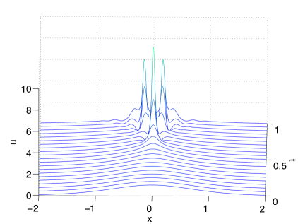
Refer to caption
Refer to caption
Figure 30: Solution to the focusing nonlocal NLS equation (5.6) for the initial data ψ0(x)=sech xsubscript𝜓0𝑥sech 𝑥\psi_{0}(x)=\mbox{sech }x and ϵ=0.1italic-ϵ0.1\epsilon=0.1; for η=0.1𝜂0.1\eta=0.1 on the left, for η=1𝜂1\eta=1 on the right. The critical time is t0=0.5subscript𝑡00.5t_{0}=0.5.

At the critical time, the tritronquée solution to PI gives as expected a much better description of the nonlocal NLS solution than the semiclassical solution as can be seen for η=0.1𝜂0.1\eta=0.1 for u𝑢u in Fig. 31. The quality of the approximation increases visibly for smaller ϵitalic-ϵ\epsilon. Note that the x𝑥x-axes are rescaled with a factor ϵ4/5superscriptitalic-ϵ45\epsilon^{4/5}.

Refer to caption
Figure 31: Solution u𝑢u to the focusing nonlocal NLS equation (5.6) for the initial data ψ0(x)=sech xsubscript𝜓0𝑥sech 𝑥\psi_{0}(x)=\mbox{sech }x and η=0.1𝜂0.1\eta=0.1 at the time t0=0.5subscript𝑡00.5t_{0}=0.5 for two values of ϵitalic-ϵ\epsilon in blue, the corresponding semiclassical solution in red and the PI solution (5.23) in green.

The corresponding plots for v𝑣v can be seen in Fig. 31. The same behavior as for u𝑢u is visible.

Refer to caption
Figure 32: Solution v𝑣v to the focusing nonlocal NLS equation (5.6) for the initial data ψ0(x)=sech xsubscript𝜓0𝑥sech 𝑥\psi_{0}(x)=\mbox{sech }x and η=0.1𝜂0.1\eta=0.1 at the time t0=0.5subscript𝑡00.5t_{0}=0.5 for two values of ϵitalic-ϵ\epsilon in blue, the corresponding semiclassical solution in red and the PI (5.23) in green.

For larger values of η𝜂\eta, the agreement is less good for both the semiclassical and the PI asymptotics. This is clear for the former since the semiclassical solution is independent of η𝜂\eta, and since the focusing effect of the nonlocal NLS is less pronounced for larger values of η𝜂\eta. The PI asymptotics takes this into account, the value of its maximum is also reduced, but more so than for the nonlocal NLS which implies that the agreement between the two solutions is best for η=0𝜂0\eta=0, i.e., the cubic NLS. The approximation gets, however, better for smaller ϵitalic-ϵ\epsilon as can be seen for η=1𝜂1\eta=1 in Fig. 33.

Refer to caption
Figure 33: Solution u𝑢u to the focusing nonlocal NLS equation (5.6) for the initial data ψ0(x)=sech xsubscript𝜓0𝑥sech 𝑥\psi_{0}(x)=\mbox{sech }x and η=1𝜂1\eta=1 at the time t0=0.5subscript𝑡00.5t_{0}=0.5 for two values of η𝜂\eta in blue, the corresponding semiclassical solution in red and the PI solution (5.23) in green.

The corresponding plots for v𝑣v can be seen in Fig. 34.

Refer to caption
Figure 34: Solution v𝑣v to the focusing nonlocal NLS equation (5.6) for the initial data ψ0(x)=sech xsubscript𝜓0𝑥sech 𝑥\psi_{0}(x)=\mbox{sech }x and η=1𝜂1\eta=1 at the time t0=0.5subscript𝑡00.5t_{0}=0.5 for two values of ϵitalic-ϵ\epsilon in blue, the corresponding semiclassical solution in red and the PI solution (5.23) in green.

Acknowledgments. The work of B.D. and T.G. was partially supported by the European Research Council Advanced Grant FroM-PDE, by PRIN 2010-11 Grant “Geometric and analytic theory of Hamiltonian systems in finite and infinite dimensions” of Italian Ministry of Universities and Researches and by the FP7 IRSES grant RIMMP “Random and Integrable Models in Mathematical Physics”. The work of B.D. was also partially supported by the Russian Federation Government Grant No. 2010-220-01-077.

References

  • [1] G.P. Agrawal, Nonlinear Fiber Optics. Academic Press, San Diego, 2006, 4th edition.
  • [2] S. Alinhac, Blowup for Nonlinear Hyperbolic Equations. Progress in Nonlinear Differential Equations and their Applications, 17. Birkhäuser Boston, Inc., Boston, MA, 1995.
  • [3] V.I. Arnold,V.V. Goryunov, O.V. Lyashko, V.A. Vasil’ev, Singularity Theory. I. Dynamical systems. VI, Encyclopaedia Math. Sci. 6, Springer, Berlin, 1993.
  • [4] A. Arsie, P. Lorenzoni, A. Moro, Integrable viscous conservation laws, Preprint: http://xxx.lanl.gov/pdf/1301.0950.pdf.
  • [5] D. Bambusi, A. Ponno, Resonance, metastability and blow up in FPU. The Fermi-Pasta-Ulam problem, 191- 205, Lecture Notes in Phys., 728, Springer, Berlin, 2008.
  • [6] W. Bao, S. Jin and P.A. Markowich, On time-splitting spectral approximations for the Schrödinger equation in the semiclassical regime, J. Comput. Phys. 175 (2002), pp. 487–524.
  • [7] W. Bao, S. Jin and P.A. Markowich, Numerical study of time-splitting spectral discretizations of nonlinear Schrödinger equations in the semi-classical regimes, SIAM J. Sci. Comp. (2003) pp. 27–64.
  • [8] G. Benettin, A. Ponno, Time-scales to equipartition in the Fermi-Pasta-Ulam problem: finite-size effects and thermodynamic limit. J. Stat. Phys. 144, (2011), 4, 793- 812.
  • [9] H. Berland and B. Skaflestad, Solving the nonlinear Schrödinger equation using exponential integrators, Technical Report 3/05, The Norwegian Institute of Science and Technology, 2005. http://www.math.ntnu.no/preprint/.
  • [10] H. Berland, A.L. Islas, and C.M. Schober, Solving the nonlinear Schrödinger equation using exponential integrators, J. Comput. Phys., 255 (2007), pp. 284-299.
  • [11] M.V. Berry, J.F. Nye and F.J. Wright, The Elliptic Umbilic Diffraction Catastrophe, Philosophical Transactions of the Royal Society of London. Series A, 291 (1979), 453-484.
  • [12] M. Bertola, A. Tovbis, Asymptotics of orthogonal polynomials with complex varying quartic weight: global structure, critical point behaviour and the first Painlevé equation. Preprint http://xxx.lanl.gov/pdf/1108.0321.pdf.
  • [13] M. Bertola, A. Tovbis, Universality for the focusing nonlinear Schrödinger equation at the gradient catastrophe point: rational breathers and poles of the Tritronquée solution to Painlevé-I. Comm. Pure Appl. Math. 66 (2013), no. 5, 678-752.
  • [14] P. Bleher, A. Its, Semiclassical asymptotics of orthogonal polynomials, Riemann-Hilbert problem, and universality in the matrix model. Ann. of Math. 150 (1999), no. 1, 185-266.
  • [15] J. Bourgain, Global solutions of nonlinear Schrödinger equations. American Mathematical Society Colloquium Publications, 46. American Mathematical Society, Providence, RI, 1999. viii+182 pp. ISBN: 0-8218-1919-4
  • [16] P. Boutroux, Recherches sur les transcendants de M. Painlevé et l’étude asymptotique des équations différentielles du second ordre. Ann. École Norm, 30 (1913) 265 - 375.
  • [17] A. Bressan, Hyperbolic systems of conservation laws. The one-dimensional Cauchy problem. Oxford Lecture Series in Mathematics and its Applications, 20. Oxford University Press, Oxford, 2000.
  • [18] É. Brézin, E. Marinari, G. Parisi, A nonperturbative ambiguity free solution of a string model. Phys. Lett. B 242, (1990) 35–38.
  • [19] J.C. Bronski, J.N Kutz, Numerical simulation of the semiclassical limit of the focusing nonlinear Schrödinger equation. Phys. Lett., A 254 (2002) 325 - 336.
  • [20] R.J. Buckingham, P.D. Miller, The sine-Gordon equation in the semiclassical limit: Critical behavior near a separatrix. J. Anal. Math. 118, (2012), no. 2, 397- 492.
  • [21] R. Buckingham, S. Venakides, Long-time asymptotics of the nonlinear Schrödinger equation shock problem. Comm. Pure Appl. Math., Published Online 12.03.2007.
  • [22] R. Carles, WKB analysis for the nonlinear Schrödinger equation and instability results. Preprint: ArXiv:math.AP/0702318.
  • [23] H. D. Ceniceros, A semi-implicit moving mesh method for the focusing nonlinear Schrödinger equation, Comm. Pure Appl. Anal. 1 (2002), pp. 1-18.
  • [24] H.D. Ceniceros, F.-R. Tian, A numerical study of the semi-classical limit of the focusing nonlinear Schrödinger equation. Phys. Lett. A 306 (2002) 25–34.
  • [25] T. Claeys, T. Grava, Universality of the break-up profile for the KdV equation in the small dispersion limit using the Riemann-Hilbert approach. Comm. Math. Phys. 286 (2009), no. 3, 979-1009.
  • [26] T. Claeys, M. Vanlessen, Universality of a double scaling limit near singular edge points in random matrix models. Comm. Math. Phys. 273 (2007), no. 2, 499-532.
  • [27] T. Claeys, M. Vanlessen, The existence of a real pole-free solution of the fourth order analogue of the Painlevé-I equation. Nonlinearity 20 (2007), no. 5, 1163-1184.
  • [28] C. Conti, A. Fratalocchi, M. Peccianti, G. Ruocco and S. Trillo, Observation of a gradient catastrophe generating solitons, Phys. Rev. Letters, 102, (2009), 083902.
  • [29] O. Costin, Correlation between pole location and asymptotic behavior for Painlevé-I solutions. Comm. Pure Appl. Math. 52 (1999) 461–478.
  • [30] O. Costin, M. Huang, S. Tanveer, Proof of the Dubrovin conjecture and analysis of the tritronqué solutions of PI. Preprint http://arxiv.org/abs/1209.1009.
  • [31] M.C. Cross and P.C. Hohenberg, Pattern formation outside of equilibrium. Rev. Mod. Phys. 65 (1993) 851-1112.
  • [32] A. de Bouard, Analytic solutions to nonelliptic nonlinear Schrödinger equations. J. Differential Equations, 104, (1993), no. 1, 196- 213.
  • [33] L. Degiovanni, F. Magri, F.V. Sciacca, On deformation of Poisson manifolds of hydrodynamic type. Comm. Math. Phys. 253 (2005), no. 1, 1- 24.
  • [34] P. Deift, Orthogonal Polynomials and Random Matrices: A Riemann-Hilbert Approach, Courant Lecture Notes 3, New York University 1999.
  • [35] P. Deift, T. Kriecherbauer, K.T-R McLaughlin, S. Venakides, and X. Zhou, Uniform asymptotics for polynomials orthogonal with respect to varying exponential weights and applications to universality questions in random matrix theory, Comm. Pure Appl. Math. 52 (1999), 1335-1425.
  • [36] P. Deift, T. Kriecherbauer, K.T-R McLaughlin, S. Venakides, and X. Zhou, Strong asymptotics of orthogonal polynomials with respect to exponential weights, Comm. Pure Appl. Math. 52 (1999), 1491-1552.
  • [37] P. Deift, K. T-R McLaughlin, A continuum limit of the Toda lattice. Mem. Amer. Math. Soc. 131 (1998), no. 624, x+216 pp.
  • [38] P. Deift, S. Venakides, X. Zhou, New results in small dispersion KdV by an extension of the steepest descent method for Riemann-Hilbert problems. Internat. Math. Res. Notices, 6, 1997, 286- 299.
  • [39] P. Deift, X.Zhou, Perturbation theory for infinite-dimensional integrable systems on the line. A case study. Acta Math. 188 (2002), no. 2, 163 262.
  • [40] A. Degasperis, Multiscale expansion and integrability of dispersive wave equations. Integrability, Lecture Notes in Phys., 767, Springer, Berlin, 2009, pp 215- 244.
  • [41] J. DiFranco, P.D. Miller, The semiclassical modified nonlinear Schrödinger equation. I. Modulation theory and spectral analysis. Phys. D 237, (2008), no. 7, 947-997.
  • [42] T. Driscoll, A composite Runge-Kutta Method for the spectral Solution of semilinear PDEs, Journal of Computational Physics, 182, (2002), 357-367.
  • [43] B. Dubrovin, On Hamiltonian perturbations of hyperbolic systems of conservation laws, II: universality of critical behaviour, Comm. Math. Phys. 267 (2006) 117 - 139.
  • [44] B. Dubrovin, On universality of critical behaviour in Hamiltonian PDEs. Geometry, topology, and mathematical physics, pp 59-109, Amer. Math. Soc. Transl. Ser. 2, 224, Amer. Math. Soc., Providence, RI, 2008.
  • [45] B. Dubrovin, M. Elaeva, On the critical behavior in nonlinear evolutionary PDEs with small viscosity. Russ. J. Math. Phys. 19 (2012), no. 4, 449-460.
  • [46] B. Dubrovin, T. Grava, C. Klein, On universality of critical behavior in the focusing nonlinear Schrödinger equation, elliptic umbilic catastrophe and the tritronquée solution to the Painlevé-I equation. J. Nonlinear Sci. 19 (2009), no. 1, 57-94.
  • [47] B. Dubrovin, T. Grava and C. Klein, Numerical Study of break-up in generalized Korteweg-de Vries and Kawahara equations, SIAM J. Appl. Math., 71, (2011), 983-1008.
  • [48] B. Dubrovin, S.-Q. Liu, Y. Zhang, On Hamiltonian perturbations of hyperbolic systems of conservation laws I: quasitriviality of bihamiltonian perturbations. Comm. Pure Appl. Math. 59 (2006) 559-615.
  • [49] B. Dubrovin, S. Novikov, Hydrodynamics of weakly deformed soliton lattices. Differential geometry and Hamiltonian theory. Russian Math. Surveys, 44 (1989), no. 6, 35-124.
  • [50] M. Duits, A. Kuijlaars, Painlevé-I asymptotics for orthogonal polynomials with respect to a varying quartic weight. Nonlinearity 19 (2006), no. 10, 2211-2245.
  • [51] G.A. El, Resolution of a shock in hyperbolic systems modified by weak dispersion. Chaos 15 (2005), no. 3, 037103, 21 pp.
  • [52] G. Falqui, On a Camassa-Holm type equation with two dependent variables. J. Phys. A 39 (2006), no. 2, 327-342.
  • [53] A.S. Fokas, A.R. Its, and A.V. Kitaev, Discrete Painlevé equations and their appearance in quantum gravity, Comm. Math. Phys. 142, (1991), 313-344.
  • [54] M.G. Forest, J.E. Lee, Geometry and modulation theory for the periodic nonlinear Schrödinger equation. In: Oscillation Theory, Computation, and Methods of Compensated Compactness (Minneapolis, Minn., 1985), 35-69. The IMA Volumes in Mathematics and Its Applications, 2. Springer, New York, 1986.
  • [55] P. Gérard, Remarques sur l’analyse semi-classique de l’équation de Schrödinger non linéaire. Séminaire sur les équations aux Dérivées Partielles, 1992-1993, Exp. No. XIII, 13 pp., École Polytech., Palaiseau, 1993.
  • [56] E. Getzler, A Darboux theorem for Hamiltonian operators in the formal calculus of variations. Duke Math. J. 111, (2002), no. 3, 535-560.
  • [57] N. Ghofraniha, C. Conti, G. Ruocco, S. Trillo, Shocks in Nonlocal Media, Phys. Rev. Letters, 99, (2007), 043903.
  • [58] J. Ginibre, G. Velo, On a class of nonlinear Schrödinger equations. I. The Cauchy problem, general case. J. Funct. Anal. 32 (1979) 1-32.
  • [59] I.S. Gradshteyn, I.M. Ryzhik, Table of Integrals, Series, and Products. Translated from the Russian. Sixth edition. Translation edited and with a preface by A. Jeffrey and D. Zwillinger. Academic Press, Inc., San Diego, CA, 2000.
  • [60] T. Grava and C. Klein, Numerical study of the small dispersion limit of the Korteweg-de Vries equation and asymptotic solutions, Physica D, 10.1016/j.physd.2012.04.001 (2012).
  • [61] T. Grava and C. Klein, Numerical study of a multiscale expansion of KdV and Camassa-Holm equation, in Integrable Systems and Random Matrices, ed. by J. Baik, T. Kriecherbauer, L.-C. Li, K.D.T-R. McLaughlin and C. Tomei, Contemp. Math. Vol. 458, 81-99 (2008).
  • [62] T. Grava, C. Klein, Numerical solution of the small dispersion limit of Korteweg de Vries and Whitham equations. Comm. Pure Appl. Math., 60(11), 1623-1664 (2007).
  • [63] E. Grenier, Semiclassical limit of the nonlinear Schrödinger equation in small time. Proc. Amer. Math. Soc. 126 (1998) 523–530.
  • [64] P. Grinevich, S.P. Novikov, String equation. II. Physical solution. (Russian) Algebra i Analiz 6 (1994), no. 3, 118–140; translation in St. Petersburg Math. J. 6 (1995), no. 3, 553–574.
  • [65] A.G. Gurevich, L.P. Pitaevskii, Non stationary structure of a collisionless shock waves. JEPT Letters 17 (1973), 193-195.
  • [66] A. Henrici, T. Kappeler, Resonant normal form for even periodic FPU chains, J. Eur. Math. Soc. (JEMS) 11 (2009), no. 5, 1025-1056.
  • [67] M.A. Hoefer, B. Ilan, Dark solitons, dispersive shock waves, and transverse instabilities.Multiscale Model. Simul. 10 (2012), no. 2, 306-341.
  • [68] T.Y. Hou, P.D. Lax, Dispersive approximations in fluid dynamics. Comm. Pure Appl. Math. 44 (1991) 1-40.
  • [69] A.M. Il’in, Matching of Asymptotic Expansions of Solutions of Boundary Value Problems. AMS Translations of Mathematical Monographs, Vol. 102, 1992; 281 pp
  • [70] E.L. Ince, Ordinary Differential Equations. Dover Publications, New York, 1944.
  • [71] S. Jin, C.D. Levermore, D.W. McLaughlin, The behavior of solutions of the NLS equation in the semiclassical limit. Singular Limits of Dispersive Waves (Lyon, 1991), 235–255, NATO Adv. Sci. Inst. Ser. B Phys., 320, Plenum, New York, 1994.
  • [72] S. Jin, C.D. Levermore, D.W. McLaughlin, The semiclassical limit of the defocusing NLS hierarchy. Comm. Pure Appl. Math. 52 (1999) 613–654.
  • [73] N. Joshi, A. Kitaev, On Boutroux’s tritronquée solutions of the first Painlevé equation. Stud. Appl. Math. 107 (2001) 253–291.
  • [74] S. Kamvissis, Long time behavior for the focusing nonlinear Schrödinger equation with real spectral singularities. Comm. Math. Phys. 180 (1996) 325–341.
  • [75] S. Kamvissis, K.D.T.-R. McLaughlin, P.D. Miller, Semiclassical Soliton Ensembles for the Focusing Nonlinear Schrödinger Equation. Annals of Mathematics Studies, 154. Princeton University Press, Princeton, NJ, 2003.
  • [76] A.A. Kapaev, Weakly nonlinear solutions of the equation P12subscriptsuperscriptP21{\rm P}^{2}_{1}, Zap. Nauchn. Sem. Leningrad. Otdel. Mat. Inst. Steklov. (LOMI) 187 (1991), Differentsialnaya Geom. Gruppy Li i Mekh. 12, 88–109, 172–173, 175; translation in J. Math. Sci. 73 (1995), no. 4, 468-481.
  • [77] A. Kapaev, Quasi-linear Stokes phenomenon for the Painlevé first equation. J. Phys. A: Math. Gen. 37 (2004) 11149-11167.
  • [78] A. Kapaev, C. Klein and T. Grava, On the tritronquée solutions of P2Isuperscriptsubscriptabsent𝐼2{}_{I}^{2}, preprint (2013) arXiv:1306.6161
  • [79] V. Kudashev, B. Suleimanov, A soft mechanism for the generation of dissipationless shock waves, Phys. Lett. A 221 (1996) 204–208.
  • [80] A.-K. Kassam and L. Trefethen, Fourth-Order Time-Stepping for stiff PDEs, SIAM J. Sci. Comput., 26 (2005), pp. 1214-1233.
  • [81] C.E. Kenig and F. Merle, Global well-posedness, scattering and blow-up for the energy-critical, focusing, non-linear Schrödinger equation in the radial case. Invent. Math. 166, (2006), no. 3, 645-675.
  • [82] A. Kitaev, The isomonodromy technique and the elliptic asymptotics of the first Painlevé transcendent. Algebra i Analiz 5 (1993), no. 3, 179–211; translation in St. Petersburg Math. J. 5 (1994), no. 3, 577–605.
  • [83] C. Klein, Fourth-Order Time-Stepping for low Dispersion Korteweg-de Vries and nonlinear Schrödinger Equation, Electronic Transactions on Numerical Analysis., 39 (2008), pp. 116-135.
  • [84] Y. Kodama, A. Mikhailov, Obstacles to asymptotic integrability, Algebraic aspects of integrable systems, 173–204, Progr. Nonlinear Differential Equations Appl., 26, Birkhäuser, Boston, MA, 1997.
  • [85] D. Kong, Formation and propagation of singularities for 2×2222\times 2 quasilinear hyperbolic systems. Trans. Amer. Math. Soc. 354, (2002), no. 8, 3155 3179.
  • [86] R. Krasny, A study of singularity formation in a vortex sheet by the point-vortex approximation. J. Fluid Mech. 167 (1986) 65–93.
  • [87] J.C. Lagarias, J.A. Reeds, M.H. Wright, and P. E. Wright, Convergence properties of the Nelder-Mead simplex method in low dimensions. SIAM Journal of Optimization 9 (1988) 112-147.
  • [88] P. Lax, D. Levermore, The small dispersion limit of the Korteweg-de Vries equation. I, II, III. Comm. Pure Appl. Math. 36 (1983) 253–290, 571–593, 809–829.
  • [89] P.D. Lax, C.D. Levermore, S. Venakides, The generation and propagation of oscillations in dispersive initial value problems and their limiting behavior. In: Important Developments in Soliton Theory, 205–241, Springer Ser. Nonlinear Dynam., Springer, Berlin, 1993.
  • [90] S.-Q. Liu, C.-Z. Wu, Y. Zhang, On properties of Hamiltonian structures for a class of evolutionary PDEs, Lett. Math. Phys. 84 (2008), no. 1, 47 63.
  • [91] S.-Q. Liu, Y. Zhang, On Quasitriviality and Integrability of a Class of Scalar Evolutionary PDEs, J. Geom. Phys. 57 (2006) 101-119.
  • [92] P. Lorenzoni, S. Paleari, Metastability and dispersive shock waves in the Fermi-Pasta-Ulam system. Phys. D 221 (2006), no. 2, 110-117.
  • [93] F. Linares, G. Ponce, Introduction to nonlinear dispersive equations. Universitext. Springer, New York, 2009. xii+256 pp. ISBN: 978-0-387-84898-3
  • [94] G.D. Lyng, P.D. Miller, The N𝑁N-soliton of the focusing nonlinear Schrödinger equation for N𝑁N large. Comm. Pure Appl. Math. 60 (2007) 951-1026.
  • [95] S.V. Manakov, P.M. Santini, On the dispersionless Kadomtsev-Petviashvili equation in n+1 dimensions: exact solutions, the Cauchy problem for small initial data and wave breaking. J. Phys. A 44 (2011), no. 40, 405203, 15 pp.
  • [96] L. Martínez-Alonso, E. Medina, Regularization of Hele-Shaw flows , multiscaling expansions and the Painlevé-I equation, Chaos Solitons Fractals, 41 (2009), no. 3, 1284-1293.
  • [97] D. Masoero, A. Raimondo, Semiclassical limit for generalized KdV equations before the gradient catastrophe. Lett. Math. Phys. 103 (2013), no. 5, 559-583.
  • [98] P.D. Miller, Z. Xu,   The Benjamin-Ono hierarchy with asymptotically reflectionless initial data in the zero-dispersion limit. Commun. Math. Sci. 10, (2012), no. 1, 117-130.
  • [99] F. Merle, P. Raphael, On universality of blow-up profile for L2superscript𝐿2L^{2} critical nonlinear Schrödinger equation, Invent. math. 156, 565-672 (2004).
  • [100] G. Métivier, Remarks on the well-posedness of the nonlinear Cauchy problem. Geometric analysis of PDE and several complex variables, 337 356, Contemp. Math., 368, Amer. Math. Soc., Providence, RI, 2005.
  • [101] P.D. Miller, S. Kamvissis, On the semiclassical limit of the focusing nonlinear Schrödinger equation. Phys. Lett. A 247 (1998) 75–86.
  • [102] G. Moore, Geometry of the string equations, Comm. Math. Phys. 133 (1990) 261-304.
  • [103] A.C. Newell, Solitons in Mathematics and Physics. CBMS-NSF Regional Conference Series in Applied Mathematics, 48. SIAM, Philadelphia, PA, 1985.
  • [104] S.P. Novikov, S.V. Manakov, L.P. Pitaevskiĭ, V.E. Zakharov, Theory of Solitons. The Inverse Scattering Method. Translated from the Russian. Contemporary Soviet Mathematics. Consultants Bureau [Plenum], New York, 1984.
  • [105] P.D. Rasmussen, O. Bang, W. Krolikowski, Theory of nonlocal soliton interaction in nematic liquid cristals, Phys. Rev. E, 72, (2005), 066611.
  • [106] J. Satsuma and N. Yajima, Initial value problems of one-dimensional self-modulation of nonlinear waves in dispersive media, Supp. Prog. Theo. Phys. 55 (1974), 284-306.
  • [107] D. Serre, Systèmes de lois de conservation I : hyperbolicité, entropies, ondes de choc; Systèmes de lois de conservation II: structures géométriques, oscillation et problèmes mixtes, Paris Diderot Editeur 1996.
  • [108] A.B. Shabat, One-dimensional perturbations of a differential operator, and the inverse scattering problem. In: Problems in Mechanics and Mathematical Physics, 279–296. Nauka, Moscow, 1976.
  • [109] L.F. Shampine, M.W. Reichelt and J. Kierzenka, Solving Boundary Value Problems for Ordinary Differential Equations in MATLAB with bvp4c, available at http://www.mathworks.com/bvp_tutorial
  • [110] P. Sikivie, The caustic ring singularity. Phys. Rev. D60 (1999) 063501.
  • [111] M. Slemrod, Monotone increasing solutions of the Painlevé 1 equation y′′=y2+xsuperscript𝑦′′superscript𝑦2𝑥y^{\prime\prime}=y^{2}+x and their role in the stability of the plasma-sheath transition. European J. Appl. Math. 13 (2002) 663–680.
  • [112] I.A.B. Strachan, Deformations of the Monge/Riemann hierarchy and approximately integrable systems, J. Math. Phys. 44 (2003) 251–262.
  • [113] C. Sulem, P. Sulem, The nonlinear Schrödinger equation. Self-focusing and wave collapse. Applied Mathematical Sciences, 139. Springer-Verlag, New York, 1999.
  • [114] T. Tao, Why are soliton stable? Bull. Amer. Math. Soc. 46 (2009), no. 1, 1 33.
  • [115] T. Tao, Nonlinear dispersive equations. Local and global analysis. CBMS Regional Conference Series in Mathematics, 106. Published for the Conference Board of the Mathematical Sciences, Washington, DC; by the American Mathematical Society, Providence, RI, 2006.
  • [116] R. Thom, Structural Stability and Morphogenesis: An Outline of a General Theory of Models. Reading, MA: Addison-Wesley, 1989.
  • [117] F.R. Tian, The initial value problem for the Whitham averaged system. Comm. Math. Phys. 166 (1994), no. 1, 79-115.
  • [118] F.R. Tian, J. Ye, On the Whitham equations for the semiclassical limit of the defocusing nonlinear Schrödinger equation. Comm. Pure Appl. Math. 52 (1999), no. 6, 655-692.
  • [119] A. Tovbis, S. Venakides, X. Zhou, On semiclassical (zero dispersion limit) solutions of the focusing nonlinear Schrödinger equation. Comm. Pure Appl. Math. 57 (2004) 877–985.
  • [120] A. Tovbis, S. Venakides, X. Zhou, On the long-time limit of semiclassical (zero dispersion limit) solutions of the focusing nonlinear Schödinger equation: pure radiation case. Comm. Pure Appl. Math. 59 (2006) 1379–1432.
  • [121] L. Trefethen, Spectral Methods in MATLAB, vol. 10 of Software, Environments, and Tools, Society for Industrial and Applied Mathematics (SIAM), Philadelphia, PA, 2000.
  • [122] S. Tsarev, The geometry of Hamiltonian systems of hydrodynamic type. The generalized hodograph method, Math. USSR Izv. 37 (1991), 397–419.
  • [123] Y. Tsutsumi, L2superscript𝐿2L^{2}-solutions for nonlinear Schrödinger equations and nonlinear groups. Funkcial. Ekvac. 30 (1987) 115–125.
  • [124] S. Venakides, The Korteweg-de Vries equation with small dispersion: higher order Lax-Levermore theory. Comm. Pure Appl. Math. 43 (1990), no. 3, 335-361.
  • [125] G.B. Whitham, Linear and Nonlinear Waves. Wiley-Intersci. 1974.
  • [126] H. Whitney, On singularities of mappings of euclidean spaces. I. Mappings of the plane into the plane. Ann. of Math. (2) 62 (1955), 374–410.
  • [127] N. Zabusky, M. Kruskal, Interaction of ”Solitons” in a Collisionless Plasma and the Recurrence of Initial States Phys. Rev. Lett. 15 (1965) 2403.
  • [128] V.E. Zakharov, A.B. Shabat, A. B. Exact theory of two-dimensional self-focusing and one-dimensional self-modulation of waves in nonlinear media. Soviet Physics JETP 34 (1972), no. 1, 62-69.; translated from Ž. Eksper. Teoret. Fiz. 1 (1971), 118-134.

Boris Dubrovin
SISSA, Via Bonomea 265, 34136 Trieste, Italy
Steklov Math. Institute, Moscow, and N.N.Bogolyubov Laboratory of Geometric Methods in Mathematical Physics
Moscow State University, 119899 Moscow, Russia
e-mail: dubrovin@sissa.it

Tamara Grava
SISSA, Via Bonomea 265, 34136 Trieste, Italy
and School of Mathematics, University of Bristol, Bristol BS8 1TW, UK
e-mail: grava@sissa.it

Christian Klein
Institut de Mathématiques de Bourgogne, Université de Bourgogne,
9 avenue Alain Savary, 21078 Dijon, Cedex, France
e-mail: Christian.Klein@u-bourgogne.fr

Antonio Moro
Department of Mathematics and Information Sciences,
University of Northumbria at Newcastle upon Tyne,
Pandon building, Camden street, NE2 1XE, Newcastle upon Tyne, UK
e-mail: antonio.moro@northumbria.ac.uk