Hyperkähler Metrics from Monopole Walls

Abstract

We present ALH hyperkähler metrics induced from well-separated $\mathrm{SU}(2)$ monopole walls which are equivalent to monopoles on $T^{2}\times\mathbb{R}$. The metrics are explicitly obtained due to Manton’s observation by using monopole solutions. These are doubly-periodic and have the modular invariance with respect to the complex structure of the complex torus $T^{2}$. We also derive metrics from monopole walls with Dirac-type singularities.

I Introduction

Hyperkähler manifolds have played important roles in the study of supersymmetric quantum field theories and string theories, especially, in the context of the string compactifications, duality tests and so on. The explicit metric on a compact hyperkähler manifold is not known except trivial examples. On the other hand, explicit forms of the non-compact hyperkähler metric have been derived in several ways. Among them the most systematic one is the hyperkähler quotient construction HKLR (see also GGR ). In 4-dimensions, the hyperkähler metrics satisfy the self-dual Einstein equations and arise as the gravitational instanton solutions (see e.g. EGH ). These can be classified into some categories: the ALE, ALF, ALG and ALH spaces Cherkis according to their asymptotic volume growth.

In the context of 3-dimensional gauge theories, hyperkähler metrics are obtained by considering well-separated monopoles, which is due to Manton’s observation Manton that the dynamics of $k$ well-separated BPS monopoles can be approximated as a geodesic motion on the asymptotic moduli space of the BPS $k$-monopole if the initial velocities of each monopole are substantially small. In this paper we only consider the case with the gauge group $\mathrm{SU}(2)$ or $\mathrm{U}(2)$.

For a non-periodic BPS $k$-monopole the moduli space can be written as $\mathcal{M}_{k}=\mathbb{R}^{3}\times(S^{1}\times\widetilde{\mathcal{M}}_{k}^{0})/\mathbb{Z}_{k}$, where the simply-connected part is denoted by $\widetilde{\mathcal{M}}_{k}^{0}$, and the degrees of $\mathbb{R}^{3}$ and $S^{1}$ correspond to the center of mass and the gauge degree of global $\mathrm{U}(1)$, respectively. The dimensions of the $k$-monopole moduli $\mathcal{M}_{k}$ is equal to $4k$. The moduli space $\mathcal{M}_{k}$ can be identified with the moduli space of a vacuum on the Coulomb branch of the three dimensional $\mathrm{SU}(k)$ super Yang-Mills theory with eight supercharges SeWi . The relative moduli space of the 2-monopole $\widetilde{\mathcal{M}}_{2}^{0}$ is known as the Atiyah-Hitchin manifold AtHi which is the ALF space with $S^{1}$ fibration over $\mathbb{R}^{3}$. In the case of well-separated BPS monopoles, each monopole carries three moduli of the position and a degree of the $\mathrm{U}(1)$ phase modulus. The latter degree corresponds to the electric charge and hence we should include the electrical degree of the dyon. The effective dynamics of the $k$-dyon system can be described by a sigma model Lagrangian whose target space is the monopole moduli space. Hence the asymptotic metric of the moduli space of the BPS $k$-monopoles can be obtained by calculating the Lagrangian of interactions of $k$ well-separated BPS monopoles (dyons). The metric is known as the Gibbons-Manton metric GiMa .

For a periodic BPS $k$-monopole on $\mathbb{R}^{2}\times S^{1}$, which is called the monopole chain Ward2005 ; ChKa2001 ; ChKa2003 , the moduli space is identified with the moduli space of a vacuum on the Coulomb branch of the four dimensional $\mathrm{SU}(k)$ super Yang-Mills theory compactified on $S^{1}$ with eight supercharges. The relative moduli space of the 2-monopole $\widetilde{\mathcal{M}}_{2}^{0}$ is the ALG space ChKa2003 . Since the periodicity is achieved by a chain of monopoles, the total energy would diverge due to the infinite number of monopoles. However, the Nahm transform can be make well-defined and the asymptotic metric of the moduli space of monopole chains is obtained in the same manner as the non-periodic case ChKa2002 . The geodesic motion is also discussed HaWa ; Maldonado ; MaWa ; Maldonado2 .

Periodicity of monopole	Super Yang-Mills theory	Asymptotic behavior (4d topology)
$\mathbb{R}^{3}$ (non-periodic)	$\mathcal{N}=4$ SYM on $\mathbb{R}^{3}$	ALF : $S^{1}$ fibration on $\mathbb{R}^{3}$
$S^{1}\times\mathbb{R}^{2}$ (periodic)	$\mathcal{N}=2$ SYM on $\mathbb{R}^{3}\times S^{1}$	ALG : $T^{2}$ fibration on $\mathbb{C}$
$T^{2}\times\mathbb{R}$ (doubly-periodic)	$\mathcal{N}=1$ SYM on $\mathbb{R}^{3}\times T^{2}$	ALH : $T^{3}$ fibration on $\mathbb{R}$

Table 1: The correspondence of the periodicity of monopole, super Yang-Mills theory and the asymptotic behavior of hyperkähler metric.

For a doubly-periodic BPS $k$-monopole on $T^{2}\times\mathbb{R}$, which is called the monopole sheet or wall Ward2005 ; Ward2007 (see also Lee ), the moduli space is identified with the moduli space of a vacuum on the Coulomb branch of the five dimensional $\mathrm{SU}(k)$ super Yang-Mills theory compactified on $T^{2}$ with eight supercharges HaVa . One of the examples of the correspondence between the monopole moduli and the vacuum moduli of the five dimensional super Yang-Mills theory is that the number of the Dirac-type singularity corresponds to that of the matter flavor. Asymptotically the relative moduli space of the monopole walls is expected to be the ALH space with $T^{3k-3}$ fibration over $\mathbb{R}^{k-1}$. As far as we know, there are no examples of ALH hyperkähler metrics in the literature except for the classical metric derived from the effective action of the $\mathcal{N}=1$ super Yang-Mills theory on $\mathbb{R}^{3}\times T^{2}$ by Haghighat and Vandoren HaVa . Furthermore, the doubly-periodic monopoles have rich properties on the D-brane interpretation, string duality, and M-theoretic interpretation via the various S,T-duality transformations ChWa . Therefore the analysis of the moduli metric would be applied to various situation of the corresponding super Yang-Mills theory, string theory and M-theory.

In this Letter, we derive some asymptotic metrics of the monopole walls on $T^{2}\times\mathbb{R}$ by calculating the effective sigma model Lagrangian of $k$ well-separated BPS walls following Manton’s observation. In our calculation, the BPS wall is assumed to be a doubly-periodic superposition of BPS monopoles in flat three-space. In the non-periodic direction, the walls are assumed to be well-separated to each other compared with the thickness of the monopole wall so that the fields can be well-approximated by superpositions of linearized monopole walls. The metric computed in this paper is for the case of two identical nonabelian monopole walls, including in the presence of Dirac singularities as well. We prove that the induced metrics actually have the modular invariance with respect to a complex structure $\tau$ of the complex torus $T^{2}$ in addition to the expected periodicity. We also present the metrics of monopole walls with Dirac-type singularities. We see that when we consider $k$ monopole walls the maximum number of singularities is $2k$ by a simple analysis using the Newton polygon. This is consistent with the fact that in the $\mathrm{SU}(k)$ super Yang-Mills theory the number of the matter flavor has the upper bound $2k$. This bound is due to the requirement that the super Yang-Mills theory is either conformal or asymptotically free. When the bound is saturated the theory has conformal invariance.

The present metrics would be the most explicit ones of the ALH type derived from the solutions of monopole walls including the case with the Dirac-type singularities. The symmetry and other properties are consistent with the one in the corresponding super Yang-Mills theory HaVa .

II Setup

Let $x^{\alpha}:=(x,y,z)$ ($\alpha=1,2,3$) be the coordinates of the three dimensional space $T^{2}\times\mathbb{R}$ in which $x$ and $y$ are periodic: $x\sim x+1,y\sim y+1$. The Higgs field $\phi$ and the gauge field $A$ satisfy the Bogomolny equation

$$*D_{A}\mathit{\phi}=-F,$$ (1)

where $D_{A}\mathit{\phi}:=\mathrm{d}\mathit{\phi}+[A,\mathit{\phi}]$ and $F:=\mathrm{d}A+A\wedge A$. We put a condition that the asymptotic behavior of the Higgs field of an $\mathrm{SU}(2)$ solution must be ChWa

$$\mathrm{EigVal}\,\phi=2\pi\mathrm{i}Q_{\pm}z+O(1)\quad\text{as}~{}z\to\pm\infty,$$

where the constants $Q_{\pm}\in\mathbb{Z}$ are called the monopole-wall charges. These are topological charges which are related to the Chern number as

$$Q_{\pm}=\int_{T_{z}}c_{1}(E_{\pm})=\frac{\mathrm{i}}{2\pi}\int_{T_{z}}\mathrm{tr}\,F_{\pm},$$

where $T_{z}$ is the complex torus at $z$ and $E_{\pm}$ are the line bundles defined at $z\rightarrow\pm\infty$, respectively, where the monopole vector bundle $E$ splits into eigenvalues of the Higgs field as $E|_{z}=E_{+}\oplus E_{-}$ ChWa . Numerical solutions of the $\mathrm{SU}(2)$ monopole walls are studied for $(Q_{-},Q_{+})=(1,1)$ and $(0,1)$ Ward2005 ; Ward2007 . The detailed analysis of the boundary conditions and the moduli space are summarized in ChWa .

Let us introduce a standard complex structure $\tau:=\tau_{1}+\mathrm{i}\tau_{2}$ ($\tau_{1},\tau_{2}\in\mathbb{R}$) at the torus $T^{2}$ and introduce a holomorphic coordinate $\xi:=x+\tau y$. The periodicity is now represented by $\xi\sim\xi+m+\tau n$ ($m,n\in\mathbb{Z}$). By using the vector notation $\bm{x}:=(\xi,z)$, the metric on $T^{2}\times\mathbb{R}$ is represented as follows:

$$\mathrm{d}\bm{x}\cdot\mathrm{d}\bm{x} :=\frac{\nu}{\tau_{2}}(\mathrm{d}x^{2}+2\tau_{1}\mathrm{d}x\mathrm{d}y+|\tau|^{2}\mathrm{d}y^{2})+\mathrm{d}z^{2}$$

$$\phantom{:}=\frac{\nu}{\tau_{2}}|\mathrm{d}\xi|^{2}+\mathrm{d}z^{2}=:g_{\alpha\beta}\mathrm{d}x^{\alpha}\mathrm{d}x^{\beta},$$ (2)

where the volume of the torus is denoted by $\nu:=\sqrt{\det g}$ ($g:=(g_{\alpha\beta})$). Note that two dimensional metric has three independent components and we have traded them with $\tau_{1},\tau_{2}$ and $\nu$. One of the crucial features of our construction of ALH hyperkähler metrics in the following is the invariance of the metric under the modular transformation,

$$\xi\mapsto\frac{\xi}{c\tau+d},\quad\tau\mapsto\frac{a\tau+b}{c\tau+d},\quad\tau_{2}\mapsto\frac{\tau_{2}}{|c\tau+d|^{2}},$$ (3)

where $\left(\begin{smallmatrix}a&b\\ c&d\end{smallmatrix}\right)\in\mathrm{SL}(2,\mathbb{Z})$.

III Asymptotic Behavior of SU(2) Monopole Walls

For the purpose of calculating the effective Lagrangian for well-separated monopole walls, we should derive the asymptotic form of the $\mathrm{SU}(2)$ monopole walls. Let us consider $k$ well-separated monopole walls sitting at the points $\bm{a}_{j}:=(\xi_{j},z_{j})$ ($j=1,\cdots,k$). Here each monopole wall has the charge $(Q_{-},Q_{+})=(0,1)$. It can be regarded as a smooth $\mathrm{SU}(2)$ monopole arranged per unit cell Ward2007 . (It is not clear that the multi-monopole walls have the moduli of the separations, however, at least the case of $(Q_{-},Q_{+})=(1,1)$ has four-moduli Ward2005 .) If the separations $|z_{j}-z_{i}|$ are large enough compared with the thicknesses of each monopole wall, the fields are well-approximated by superpositions of linearized monopole walls:

$$\phi(\bm{x}) =v+\sum_{j=1}^{k}\phi^{j}(\bm{x}-\bm{a}_{j}),$$ (4)

$$A_{\xi}(\bm{x}) =b+\sum_{j=1}^{k}A_{\xi}^{j}(\bm{x}-\bm{a}_{j}),\quad A_{z}(\bm{x})=0,$$ (5)

where $v$ and $b$ are the vacuum expectation value of the Higgs field and the background gauge field respectively. Then we can estimate the asymptotic Higgs field of each monopole wall as a superposition of linearized ’t Hooft-Polyakov monopoles arranged in a finite $(2M+1)\times(2N+1)$ rhombic lattice,

$$\phi^{j}(\bm{x})=\frac{1}{4\pi}\sum_{m=-M}^{M}\sum_{n=-N}^{N}\frac{-g}{\sqrt{|\xi-m-n\tau|^{2}+z^{2}}},$$ (6)

where $g$ is the magnetic charge of the ’t Hooft-Polyakov monopoles. The summation would diverge in the limit of $M$ and $N$ to infinity. Such divergence can be avoided in a similar way to the case of periodic monopoles ChKa2002 . Namely, the asymptotic form of $\phi^{j}(\bm{x})$ for large $|z|$ can be written as Linton

$$\phi^{j}(\bm{x})=\frac{g}{2}|z|-gC_{M,N},$$ (7)

where $C_{M,N}$ is a positive constant diverging linearly in the limit $M,N\to\infty$. By substituting (7) into (4), we obtain

$$\phi(\bm{x})=v_{\mathrm{ren}}+\frac{g}{2}\sum_{j=1}^{k}|z-z_{j}|,$$ (8)

where $v_{\mathrm{ren}}:=v-kgC_{M,N}$, which can be kept finite with $v$ diverging at the same order as $C_{M,N}$. We note that the configuration is not localized in the periodic directions. This implies that the superposition of doubly-periodic monopoles is represented as a constituent monopole wall in the asymptotic region.

The asymptotic gauge field can also be derived from the Bogomolny equation with (7),

$$A_{\xi}^{j}(\bm{x})=\frac{\mathrm{i}\nu g}{8\tau_{2}}\,\mathrm{sign}(z)\,\bar{\xi},\quad A_{z}^{j}(\bm{x})=0,$$ (9)

where

$$\mathrm{sign}(z):=\left\{\begin{array}[]{rl}+1&(z>0)\\ -1&(z<0)\end{array}\right..$$ (12)

In order to make the gauge field doubly-periodic for $\xi\to\xi+m+\tau n$, we have to perform appropriate gauge transformations. This means our $\mathrm{U}(1)$ bundle over the complex torus is non-trivial. Accordingly we have to impose the following twisted boundary condition where the phase $\theta$ of any functions in the fundamental representation of the gauge group shifts as follows; (cf. Eq. (12) in Ward2005 ):

$$\theta \mapsto\theta+\frac{\nu g}{4}\,\mathrm{sign}(z)\,y\quad\text{when}\quad\xi\mapsto\xi+1,$$ (13)

$$\theta \mapsto\theta-\frac{\nu g}{4}\,\mathrm{sign}(z)\,x\quad\text{when}\quad\xi\mapsto\xi+\tau.$$ (14)

For later convenience we introduce the following pair of the harmonic function and the Dirac potential on $T^{2}\times\mathbb{R}$

$$u(z)=\frac{1}{2}|z|-C_{M,N},\quad w(\bm{x})=\frac{\mathrm{i}\nu}{8\tau_{2}}\,\mathrm{sign}(z)\,\bar{\xi},$$ (15)

which satisfy $u(z)=u(-z)$ and $w(\bm{x})=w(-\bm{x})$. Note that $u(z)$ is a harmonic function on $\mathbb{R}$ with $\delta$-function source at the origin.

IV Asymptotic Metric from SU(2) Monopole Walls

As mentioned in the introduction, the interaction of non-static monopoles involves not only the relative coordinates but also the relative phases. The relative phase factor gives rise to non vanishing electric charges and hence converts monopoles into dyons. The interaction term of the Lagrangian can be obtained from the analysis of the forces between BPS monopoles. The fact that there is no force between well-separated BPS monopoles with the same charge implies the existence of a long-range interaction caused by the Higgs field which becomes massless in the BPS limit. This is also the case for dyons. Thus the Lagrangian of the $\ell^{\mathrm{th}}$ monopole wall can be written as

$$L_{\ell} =-(g^{2}+q_{\ell}^{2})^{1/2}\phi(1-\bm{V}_{\ell}^{2})^{1/2}$$

$$+q_{\ell}\bm{V}_{\ell}\cdot\bm{A}-q_{\ell}A_{0}+g\bm{V}_{\ell}\cdot\tilde{\bm{A}}-g\tilde{A}_{0},$$ (16)

where $(g^{2}+q_{\ell}^{2})^{1/2}$, $q_{\ell}$ and $\bm{V}_{\ell}:=(\dot{\xi}_{\ell},\dot{z}_{\ell})$ are the scalar charge, the electric charge and the velocity of $\ell^{\mathrm{th}}$ monopole wall respectively. Note that all the particles have the same magnetic charge $g$, while the electric charges $q_{\ell}$ may change particle by particle in general. The first term of the Lagrangian gives rise to the scalar interaction due to the Higgs field. The second and the third terms are the ordinary Lorentz force. The remaining terms describe the dual magnetic interaction to the electric Lorentz force. The relevant field is the dual potential $(\tilde{\bm{A}},\tilde{A}_{0})$ which satisfies $\tilde{F}=*F$. The background fields $\phi$, $\bm{A}$, $A_{0}$, $\tilde{\bm{A}}$ and $\tilde{A}_{0}$ are generated by the remaining $(k-1)$ moving dyons, which can be obtained from the solutions derived in the previous section. For $j\neq\ell$, the asymptotic fields of $j^{\mathrm{th}}$ dyonic monopole wall at rest can be derived in the same way as the non-periodic monopoles,

$$\phi^{j}(\bm{x}) =(g^{2}+q_{j}^{2})^{1/2}u(z),$$ (17)

$$A_{\xi}^{j}(\bm{x}) =gw(\bm{x}), \quad\tilde{A}_{\xi}^{j}(\bm{x}) =-q_{j}w(\bm{x}),$$

$$A_{z}^{j}(\bm{x}) =0, \quad\tilde{A}_{z}^{j}(\bm{x}) =0,$$

$$A_{0}^{j}(\bm{x}) =-q_{j}u(z), \quad\tilde{A}_{0}^{j}(\bm{x}) =-gu(z),$$ (18)

where $u(z)$ and $w(\bm{x})$ for the monopole wall are given by (15). Then the fields for a moving monopole can be obtained by the Lorentz boost. Keeping the terms of order $q_{j}^{2}$, $q_{j}\bm{V}_{j}$ and $\bm{V}_{j}^{2}$, we find

$$\phi^{j}(\bm{x}) \simeq(g^{2}+q_{j}^{2})^{1/2}u(z)(1-\bm{V}_{j}^{2})^{1/2},$$ (19)

$$A_{\xi}^{j}(\bm{x}) \simeq-q_{j}u(z)V_{j\xi}+gw(\bm{x}),$$

$$A_{z}^{j}(\bm{x}) \simeq-q_{j}u(z)V_{jz},$$

$$A_{0}^{j}(\bm{x}) \simeq-q_{j}u(z)+g(wV_{j}^{\xi}+\bar{w}V_{j}^{\bar{\xi}}),$$

$$\tilde{A}_{\xi}^{j}(\bm{x}) \simeq-gu(z)V_{j\xi}-q_{j}w(\bm{x}),$$

$$\tilde{A}_{z}^{j}(\bm{x}) \simeq-gu(z)V_{jz},$$

$$\tilde{A}_{0}^{j}(\bm{x}) \simeq-gu(z)-q_{j}(wV_{j}^{\xi}+\bar{w}V_{j}^{\bar{\xi}}),$$ (20)

where the scalar potentials are replaced by the Liénard-Wiechert potentials with the approximation of the distance $(r^{2}-|\bm{r}\times\bm{V}|^{2}+O(\bm{V}^{2}))^{1/2}$ by $r$.

Substituting (20) into the Lagrangian for $k=2$ and keeping terms of the second order in $q_{1}$, $\bm{V}_{1}$, $q_{2}$ and $\bm{V}_{2}$, we obtain

$$L_{2} =-m_{2}+\frac{1}{2}m_{2}\bm{V}_{2}^{2}+q_{2}(bV_{2}^{\xi}+\bar{b}V_{2}^{\bar{\xi}})$$

$$+\frac{g^{2}}{2}u(z_{2}-z_{1})(\bm{V}_{2}-\bm{V}_{1})^{2}-\frac{1}{2}u(z_{2}-z_{1})(q_{2}-q_{1})^{2}$$

$$+g(q_{2}-q_{1})\big{\{}w_{21}(V_{2}^{\xi}-V_{1}^{\xi})+\bar{w}_{21}(V_{2}^{\bar{\xi}}-V_{1}^{\bar{\xi}})\big{\}},$$ (21)

where $m_{j}:=v(g+q_{j})^{1/2}$ is the rest mass of the $j^{\mathrm{th}}$ monopole wall and $w_{ji}:=w(\bm{x}_{j}-\bm{x}_{i})$. Furthermore, expanding $m_{j}$ and making symmetrization, we obtain the total Lagrangian $L_{21}$ as

$$L_{21} =\frac{vg}{2}(\bm{V}_{2}^{2}+\bm{V}_{1}^{2})+\frac{g^{2}}{2}u(z_{2}-z_{1})(\bm{V}_{2}-\bm{V}_{1})^{2}$$

$$-\frac{v}{2g}(q_{2}^{2}+q_{1}^{2})-\frac{1}{2}u(z_{2}-z_{1})(q_{2}-q_{1})^{2}$$

$$+b(q_{2}V_{2}^{\xi}+q_{1}V_{1}^{\xi})+gw_{21}(q_{2}-q_{1})(V_{2}^{\xi}-V_{1}^{\xi})$$

$$+\bar{b}(q_{2}V_{2}^{\bar{\xi}}+q_{1}V_{1}^{\bar{\xi}})+g\bar{w}_{21}(q_{2}-q_{1})(V_{2}^{\bar{\xi}}-V_{1}^{\bar{\xi}}).$$ (22)

The Lagrangian may look ill-defined due to the diverging $v$, however, it can be replaced by $v_{\mathrm{ren}}$ which remains finite (cf. (7), (8), and (15)). Then the Lagrangian can be divided into the two parts: $L_{21}=L_{\mathrm{CM}}+L_{\mathrm{rel}}$, where

$$L_{\mathrm{CM}} =\frac{vg}{4}(\bm{V}_{2}+\bm{V}_{1})^{2}-\frac{v}{4g}(q_{2}+q_{1})^{2}+\frac{b}{2}(q_{2}+q_{1})(V_{2}^{\xi}+V_{1}^{\xi})+\frac{\bar{b}}{2}(q_{2}+q_{1})(V_{2}^{\bar{\xi}}+V_{1}^{\bar{\xi}}),$$ (23)

$$L_{\mathrm{rel}} =\frac{g^{2}}{2}\left(\frac{v_{\mathrm{ren}}}{2g}+\frac{1}{2}|z_{2}-z_{1}|\right)(\bm{V}_{2}-\bm{V}_{1})^{2}-\frac{1}{2}\left(\frac{v_{\mathrm{ren}}}{2g}+\frac{1}{2}|z_{2}-z_{1}|\right)(q_{2}-q_{1})^{2}$$

$$+\left\{\frac{b}{2}+\frac{\mathrm{i}\nu g}{8\tau_{2}}\,\mathrm{sign}(z_{2}-z_{1})\,(\bar{\xi}_{2}-\bar{\xi}_{1})\right\}(q_{2}-q_{1})(V_{2}^{\xi}-V_{1}^{\xi})$$

$$+\left\{\frac{\bar{b}}{2}-\frac{\mathrm{i}\nu g}{8\tau_{2}}\,\mathrm{sign}(z_{2}-z_{1})\,(\xi_{2}-\xi_{1})\right\}(q_{2}-q_{1})(V_{2}^{\bar{\xi}}-V_{1}^{\bar{\xi}}).$$ (24)

The center of mass Lagrangian $L_{\mathrm{CM}}$ would diverge while the relative Lagrangian $L_{\mathrm{rel}}$ would converge in the limit of $M,N\rightarrow\infty$. The asymptotic metric of the moduli space can be read from the relative Lagrangian. For convenience, we introduce relative variables by $\xi:=\xi_{2}-\xi_{1}$, $z:=z_{2}-z_{1}$, $\bm{V}:=\bm{V}_{2}-\bm{V}_{1}$ and $q:=q_{2}-q_{1}$ and further replace the electric charge $q$ in $L_{\mathrm{rel}}$ by the relative phase $\theta$ via the Legendre transformation,

$$L_{\mathrm{rel}}^{\prime}=L_{\mathrm{rel}}+q\dot{\theta}.$$ (25)

As we will see shortly the coefficient of $q\dot{\theta}$ can be fixed so that the asymptotic metric has the double periodicity. After the Legendre transformation, we obtain the asymptotic metric of the moduli space in the form of the Gibbons-Hawking ansatz GiHa ,

$$\frac{1}{g}\mathrm{d}s^{2}=U\mathrm{d}\bm{x}\cdot\mathrm{d}\bm{x}+\frac{1}{U}(\mathrm{d}\theta+\bm{W}\cdot\mathrm{d}\bm{x})^{2},$$ (26)

where

$$U=\frac{v_{\mathrm{ren}}}{2}+\frac{g}{2}|z|,\quad W_{\xi} =\frac{b}{2}+\frac{\mathrm{i}\nu g}{8\tau_{2}}\,\mathrm{sign}(z)\,\bar{\xi},$$

$$W_{\bar{\xi}} =\overline{W}_{\xi},\quad W_{z}=0.$$ (27)

At first sight the metric seems to have a constant shift when we go around the closed cycles on $T^{2}$, since $W_{\xi}$ explicitly depends on the coordinate $\bar{\xi}$. However we can confirm the double-periodicity of the metric by observing that the constant shift of $W_{\xi}$ can be cancelled by the phase shift due to the necessary $\mathrm{U}(1)$ gauge transformation in the twisted boundary conditions (13) and (14), which also determines the coefficient of $q\dot{\theta}$ in (25). Furthermore, we can also easily check the invariance of the metric under the modular transformation (3). Thus our metric (26) is well-defined on $T^{3}\times\mathbb{R}$ with local coordinates $(\theta,\xi,z)$. Finally the hyperkähler metric (26) allows the following local isometries with parameters $(\alpha,\beta,\gamma)$;

$$\theta \to\theta+\alpha+\frac{\nu g}{4}\,\mathrm{sign}(z)\,(\beta y-\gamma x),$$

$$x \to x+\beta,\qquad y\to y+\gamma.$$ (28)

It is straightforward to extend the above computation for $k=2$ to the case of general $k$. The total Lagrangian of the $k$ well-separated monopole walls can be obtained by generalizing (22) as follows

$$L_{k} =\frac{vg}{2}\sum_{j=1}^{k}\bm{V}_{j}^{2}+\frac{g^{2}}{2}\sum_{1\leq i<j\leq k}u(z_{j}-z_{i})(\bm{V}_{j}-\bm{V}_{i})^{2}$$

$$-\frac{v}{2g}\sum_{j=1}^{k}q_{j}^{2}-\frac{1}{2}\sum_{1\leq i<j\leq k}u(z_{j}-z_{i})(q_{j}-q_{i})^{2}$$

$$+b\sum_{j=1}^{k}q_{j}V_{j}^{\xi}+\sum_{1\leq i<j\leq k}gw_{ji}(q_{j}-q_{i})(V_{j}^{\xi}-V_{i}^{\xi})$$

$$+\bar{b}\sum_{j=1}^{k}q_{j}V_{j}^{\bar{\xi}}+\sum_{1\leq i<j\leq k}g\bar{w}_{ji}(q_{j}-q_{i})(V_{j}^{\bar{\xi}}-V_{i}^{\bar{\xi}}).$$ (29)

This can be decomposed into the two parts $L_{k}=L_{\mathrm{CM}}+L_{\mathrm{rel}}$, where

$$L_{\mathrm{CM}} =\frac{vg}{2k}\,\Bigg{(}\sum_{j=1}^{k}\bm{V}_{j}\Bigg{)}^{2}-\frac{v}{2kg}\,\Bigg{(}\sum_{j=1}^{k}q_{j}\Bigg{)}^{2}+\frac{b}{k}\,\Bigg{(}\sum_{j=1}^{k}q_{j}\Bigg{)}\Bigg{(}\sum_{j=1}^{k}V_{j}^{\xi}\Bigg{)}+\frac{\bar{b}}{k}\,\Bigg{(}\sum_{j=1}^{k}q_{j}\Bigg{)}\Bigg{(}\sum_{j=1}^{k}V_{j}^{\bar{\xi}}\Bigg{)},$$ (30)

$$L_{\mathrm{rel}} =\frac{g^{2}}{2}\sum_{1\leq i<j\leq k}\left(\frac{v_{\mathrm{ren}}}{kg}+\frac{1}{2}|z_{j}-z_{i}|\right)(\bm{V}_{j}-\bm{V}_{i})^{2}-\frac{1}{2}\sum_{1\leq i<j\leq k}\left(\frac{v_{\mathrm{ren}}}{kg}+\frac{1}{2}|z_{j}-z_{i}|\right)(q_{j}-q_{i})^{2}$$

$$+\sum_{1\leq i<j\leq k}\left\{\frac{b}{k}+\frac{\mathrm{i}\nu g}{8\tau_{2}}\,\mathrm{sign}(z_{j}-z_{i})\,(\bar{\xi}_{j}-\bar{\xi}_{i})\right\}(q_{j}-q_{i})(V_{j}^{\xi}-V_{i}^{\xi})$$

$$+\sum_{1\leq i<j\leq k}\left\{\frac{\bar{b}}{k}-\frac{\mathrm{i}\nu g}{8\tau_{2}}\,\mathrm{sign}(z_{j}-z_{i})\,(\xi_{j}-\xi_{i})\right\}(q_{j}-q_{i})(V_{j}^{\bar{\xi}}-V_{i}^{\bar{\xi}}).$$ (31)

On the other hand, the Gibbons-Hawking ansatz for general $k$ can be written as

$$\frac{1}{g}\mathrm{d}s^{2} =U_{IJ}\mathrm{d}\bm{X}_{I}\cdot\mathrm{d}\bm{X}_{J}+U_{IJ}^{-1}(\mathrm{d}\mathit{\Theta}_{I}+\bm{W}_{IK}\cdot\mathrm{d}\bm{X}_{K})$$

$$\qquad\qquad\qquad\qquad\cdot\,(\mathrm{d}\mathit{\Theta}_{J}+\bm{W}_{JL}\cdot\mathrm{d}\bm{X}_{L}),$$ (32)

where $I,J,K,L=1,\cdots,k-1$, and $\mathit{\Xi}_{J}:=\xi_{J}-\xi_{k}$, $Z_{J}:=z_{J}-z_{k}$, $\mathit{\Theta}_{J}:=\theta_{J}-\theta_{k}$ and $\bm{X}_{J}:=(\mathit{\Xi}_{J},Z_{J})$ are relative coordinates measured by the position of $k^{\mathrm{th}}$ monopole wall. By comparing the coefficients of (31) and the sigma model Lagrangian for the Gibbons-Hawking ansatz, we find:

$$U_{JJ} =(k-1)\frac{v_{\mathrm{ren}}}{k}+\frac{g}{2}\sum_{I\neq J}|Z_{J}-Z_{I}|,$$

$$U_{IJ} =-\frac{v_{\mathrm{ren}}}{k}-\frac{g}{2}|Z_{J}-Z_{I}|,~{}~{}\text{($I\neq J$)}$$

$$(W_{\xi})_{JJ} =(k-1)\frac{b}{k}+\frac{\mathrm{i}\nu g}{8\tau_{2}}\sum_{I\neq J}\mathrm{sign}(Z_{J}-Z_{I})\,(\bar{\mathit{\Xi}}_{J}-\bar{\mathit{\Xi}}_{I}),$$

$$(W_{\xi})_{IJ} =-\frac{b}{k}-\frac{\mathrm{i}\nu g}{8\tau_{2}}\,\mathrm{sign}(Z_{J}-Z_{I})\,(\bar{\mathit{\Xi}}_{J}-\bar{\mathit{\Xi}}_{I}),~{}~{}\text{($I\neq J$)}$$

$$(W_{\bar{\xi}})_{IJ} =(\overline{W}_{\xi})_{IJ},\quad(W_{z})_{IJ}=0.$$ (33)

V Asymptotic Metric from U(2) Monopole Walls with Singularities

Finally, we discuss the asymptotic metrics of monopole walls with Dirac-type singularities. In the case of monopole chains with four-moduli, it is proved that the maximum number of Dirac singularities is four. Here we derive the inequality for the maximum number of Dirac singularities of monopole walls by using the spectral curves and the Newton polygon ChWa .

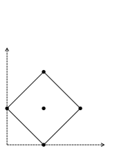
Figure 1: A Newton polygon of an $\mathrm{SU}(2)$ monopole wall with charge $Q_{\pm}=1$.

A spectral curve of a monopole wall is defined by $F_{x}:=\det[V_{x}(s)-t]$, where $V_{x}(s)$ is an integral of $(D_{x}+\mathrm{i}\phi)\psi=0$ in the $x$-direction and $s:=\exp[2\pi(z-\mathrm{i}y)]$. The spectral curve also induces a spectral polynomial $G_{x}(s,t):=P(s)F_{x}(s,t)$, where $P(s)$ is a common denominator of $F_{x}$. Then the Newton polygon $N_{x}$ of $G_{x}(s,t)$ can be constructed as follows. Firstly we mark points $(a,b)$ corresponding to the degree of each term $s^{a}t^{b}$ of $G_{x}(s,t)$ on an integer lattice. Then the Newton polygon is a minimal convex polygon including all the marks. For example, the spectral curves of the $\mathrm{SU}(2)$ monopole walls can be written as $F_{x}(s,t)=t^{2}-W_{x}(s)t+1$, where $W_{x}(s):=\mathrm{Tr}\,V_{x}(s)$, which leads to the Newton polygon of an $\mathrm{SU}(2)$ monopole wall with the charge $(Q_{-},Q_{+})=(1,1)$ as in Figure 1. In addition, the shape of the Newton polygon is restricted by the boundary data. For example, the numbers of points on top and bottom edges are equal to $r_{\pm 0}+1$, where $r_{\pm 0}$ are the number of positive and negative Dirac singularities of a $\mathrm{U}(2)$ monopole wall. Moreover, there is an important relation between the number of internal points of the Newton polygon, $\mathrm{Int}\,N_{x}$, and the dimension of the moduli space $\mathcal{M}$ of the corresponding monopole walls:

$$\dim\mathcal{M}=4\,\mathrm{Int}\,N_{x}.$$

Keeping these in mind, the upper limit of the number of singularities of $\mathrm{U}(2)$ monopoles can be easily obtained as follows. For a given number of internal points, the maximum Newton polygon of monopole walls with singularities must be a trapezoid, which has height 2 and has length of top and bottom edges $r_{+0}$ and $r_{-0}$ respectively (Figure 2).

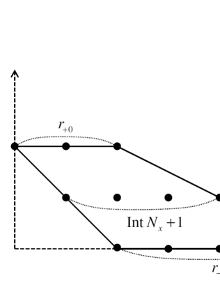
Figure 2: The maximum Newton polygon $N_{x}$ of a $\mathrm{U}(2)$ monopole wall with $r_{+0}$ singularities and $r_{-0}$ singularities.

From the shape of the Newton polygon, the maximum number of singularities obviously have a relation, $r_{+0}+r_{-0}=2(\mathrm{Int}\,N_{x}+1)$ (which can also be derived by the Pick’s formula). Thus the total number of the singularities $r_{0}:=r_{+0}+r_{-0}$ is limited as

$$r_{0}\leq\frac{1}{2}\dim\mathcal{M}+2.$$ (34)

Especially the maximum number of singularities of $k$ well-separated monopole walls is $2k$ because the dimension of the relative moduli space is $4(k-1)$. This is consistent with the fact that the maximal number of the matter hypermultiplets in the fundamental representation is $2k$ in the corresponding $\mathrm{SU}(k)$ super Yang-Mills theory with eight super charges.

Here we restrict our calculation to the monopole walls with four-moduli, that is, for $k=2$. Then the maximal number of the Dirac singularities is $r_{0}=4$. Since these singularities are stationary and have no electric charge, the metric can be obtained by simply replacing the vacuum expectation value and the background field by $v+\sum_{\ell=1}^{r_{0}}g_{\ell}u(r_{\ell z}-z)$ and $b+\sum_{\ell=1}^{r_{0}}g_{\ell}w(\bm{r}_{\ell}-\bm{x})$ respectively, where $g_{\ell}$ and $\bm{r}_{\ell}:=(r_{\ell\xi},r_{\ell z})$ are the magnetic charges and the positions of each singularity ChKa2002 . Substituting them into (27), we obtain

$$U =\frac{v_{\mathrm{ren}}^{\prime}}{2}+\frac{g}{2}|z|+\frac{1}{4}\sum_{\ell=1}^{r_{0}}g_{\ell}\left|r_{\ell z}-\frac{z}{2}\right|$$

$$\phantom{=\frac{v_{\mathrm{ren}}^{\prime}}{2}+\frac{g}{2}|z|}~{}+\frac{1}{4}\sum_{\ell=1}^{r_{0}}g_{\ell}\left|r_{\ell z}+\frac{z}{2}\right|,$$

$$W_{\xi} =\frac{b}{2}+\frac{\mathrm{i}\nu g}{8\tau_{2}}\,\mathrm{sign}(z)\,\bar{\xi}$$

$$+\frac{\mathrm{i}\nu}{16\tau_{2}}\sum_{\ell=1}^{r_{0}}g_{\ell}\,\mathrm{sign}\!\left(r_{\ell z}-\frac{z}{2}\right)\left(\bar{r}_{\ell\xi}-\frac{\bar{\xi}}{2}\right)$$

$$+\frac{\mathrm{i}\nu}{16\tau_{2}}\sum_{\ell=1}^{r_{0}}g_{\ell}\,\mathrm{sign}\!\left(r_{\ell z}+\frac{z}{2}\right)\left(\bar{r}_{\ell\xi}+\frac{\bar{\xi}}{2}\right),$$

$$W_{\bar{\xi}} =\overline{W}_{\xi},\quad W_{z}=0,$$ (35)

where

$$v_{\mathrm{ren}}^{\prime}:=v-\left(2+\sum_{\ell=1}^{r_{0}}\frac{g_{\ell}}{g}\right)gC_{M,N}$$ (36)

and we assume $\bm{x}_{1}+\bm{x}_{2}=\bm{0}$.

In the correspondence with ${\mathcal{N}}=1$ super Yang-Mills theory on $\mathbb{R}^{3}\times T^{2}$, the function $U(z)$ is identified with the low energy effective coupling, or the second derivative of the prepotential on the Coulomb modulus $\mathbb{R}_{>0}$.

VI Conclusion

In this Letter, we have obtained new hyperkähler metrics whose asymptotic behavior is the ALH type from the moduli space of monopole walls. The metric in four dimensions is defined on a $T^{2}\times S^{1}$ fibration over $\mathbb{R}$ and enjoys the modular invariance on $T^{2}$. We have also derive the maximal number of the Dirac singularities by using the Newton polygon of the spectral curve.

One of the next challenges is the low-energy scattering of the monopole walls as a geodesic motion on the moduli space. In the present discussion, the monopoles are assumed to be well-separated and hence the collision process is excluded.

In order to obtain a global metric on the moduli space of monopole walls, we need some ideas such as the one for the Atiyah-Hitchin metric AtHi for non-periodic BPS $\mathrm{SU}(2),2$-monopole. On the super Yang-Mills theory side, the region of well-separated monopoles corresponds to the weak coupling region of the moduli space of the Coulomb branch, where the vacuum expectation values of the scalar fields in the vector multiplets are large compared with the dynamical scale of the theory. In order to obtain a global metric which is valid on the whole Coulomb branch, the inclusion of instanton corrections is crucial. A successful example of such computation is the Ooguri-Vafa metric OoVa . See also GMN and Nei for recent developments.

In the periodic monopoles, the monopole scattering has been successfully discussed by using the Nahm transform, the spectral curve and the corresponding Hitchin equation HaWa ; Maldonado ; MaWa . These methods could be applied to the doubly-periodic case.

Acknowledgments

The authors thank the Yukawa Institute for Theoretical Physics at Kyoto University. Discussions during the YITP workshop on “Field Theory and String Theory” (YITP-W-13-12) were useful to complete this work. MH, HK and DM are supported in part by Grant-in-Aid for Young Scientists (#23740182), Grant-in-Aids for Scientific Research (#22224001 and #24540265) and Grant-in-Aid for JSPS Fellows, respectively.

References

• (1) N. J. Hitchin, A. Karlhede, U. Lindström and M. Ro$\check{\mbox{c}}$ek, Hyperkähler metrics and supersymmetry, Commun. Math. Phys.  108, 535 (1987).
• (2) G. W. Gibbons, P. Rychenkova and R. Goto, HyperKähler quotient construction of BPS monopole moduli spaces, Commun. Math. Phys.  186, 581 (1997), [hep-th/9608085].
• (3) T. Eguchi, P. B. Gilkey and A. J. Hanson, Gravitation, gauge theories and differential geometry, Phys. Rept.  66, 213 (1980).
• (4) S. A. Cherkis, Instantons on gravitons, Commun. Math. Phys.  306, 449 (2011), [arXiv:1007.0044 [hep-th]].
• (5) N. S. Manton, Monopole interactions at long range, Phys. Lett. B154, 397 (1985) [Erratum-ibid.  157B, 475 (1985)].
• (6) N. Seiberg and E. Witten, Gauge dynamics and compactification to three-dimensions, [hep-th/9607163].
• (7) M. F. Atiyah and N. J. Hitchin, The Geometry and Dynamics of Magnetic Monopoles, Princeton University Press (1988).
• (8) G. W. Gibbons and N. S. Manton, The moduli space metric for well-separated BPS monopoles, Phys. Lett. B356, 32 (1995), [arXiv:hep-th/9506052].
• (9) S. A. Cherkis and A. Kapustin, Nahm transform for periodic monopoles and $N=2$ super Yang-Mills theory, Commun. Math. Phys.  218, 333 (2001), [arXiv:hep-th/0006050].
• (10) S. A. Cherkis and A. Kapustin, Periodic monopoles with singularities and $N=2$ super-QCD, Commun. Math. Phys.  234, 1 (2003), [arXiv:hep-th/0011081].
• (11) R. S. Ward, Periodic monopoles, Phys. Lett. B619, 177 (2005), [arXiv:hep-th/0505254].
• (12) S. A. Cherkis and A. Kapustin, Hyperkähler metrics from periodic monopoles, Phys. Rev. D65, 084015 (2002), arXiv:hep-th/0109141.
• (13) D. Harland and R. S. Ward, Dynamics of periodic monopoles, Phys. Lett. B 675, 262 (2009) [arXiv:0901.4428 [hep-th]].
• (14) R. Maldonado, Periodic monopoles from spectral curves, JHEP 1302, 099 (2013), [arXiv:1212.4481 [hep-th]].
• (15) R. Maldonado and R. S. Ward, Geometry of periodic monopoles, arXiv:1309.7013 [hep-th].
• (16) R. Maldonado, “Higher charge periodic monopoles,” arXiv:1311.6354 [hep-th].
• (17) R. S. Ward, A monopole wall, Phys. Rev. D75, 021701 (2007), [arXiv:hep-th/0612047].
• (18) K. -M. Lee, Sheets of BPS monopoles and instantons with arbitrary simple gauge group, Phys. Lett. B445, 387 (1999), [arXiv:hep-th/9810110].
• (19) B. Haghighat and S. Vandoren, Five-dimensional gauge theory and compactification on a torus, JHEP 1109, 060 (2011), [arXiv:1107.2847 [hep-th]].
• (20) S. A. Cherkis and R. S. Ward, Moduli of monopole walls and amoebas, JHEP 1205, 090 (2012), [arXiv:1202.1294 [hep-th]].
• (21) C. M. Linton, Rapidly convergent representations for Green’ functions for Laplace’ equation, Proc. Roy. Soc. Lond. A 455, 1767 (1999).
• (22) G. W. Gibbons and S. W. Hawking, Gravitational multi - instantons, Phys. Lett. B78, 430 (1978).
• (23) H. Ooguri and C. Vafa, Summing up D instantons, Phys. Rev. Lett.  77, 3296 (1996), [hep-th/9608079].
• (24) D. Gaiotto, G. W. Moore and A. Neitzke, Four-dimensional wall-crossing via three-dimensional field theory, Commun. Math. Phys.  299, 163 (2010), [arXiv:0807.4723 [hep-th]].
• (25) A. Neitzke, Notes on a new construction of hyperkähler metrics, arXiv:1308.2198 [math.DG].