Dynamical signature of edge state in the 1D Aubry-André model
Abstract
Topological feature has become an intensively studied subject in many fields of physics. As a witness of topological phase, the edge states are topologically protected and may be helpful in quantum information processing. In this paper, we define a measure to quantify the dynamical localization of system and simulate the localization in the 1D Aubry-André model. We find an interesting connection between the edge states and the dynamical localization of the system, this connection may be used as a signature of edge state and topological phase.
pacs:
03.67.Lx, 03.65.Vf, 71.10.PmI introduction
The discovery of topological insulators has attracted considerable attention in the field of topological phases of matter Bernevig ; Fu ; Koenig ; Hsieh1 ; Chen ; Xia ; Hsieh2 ; Kuroda . Earlier studies in this field mainly focus on three issues, (1) topological properties of the ground state phases, (2) realizations of topological quantum matteryao13 , and (3) possible applications of topological matter, e.g., applications of edge states for topological quantum computing and spintronicsnayak08 ; moore10 . Yet, explorations on the dynamical feature of topological quantum matter are scarce. This motivates the study in this paper.
Localization induced by disorder has been recently observed in ultracold bosonic gases in purely random potentials roati08 and in bichromatic optical latticebilly08 . In both systems, the observations have been interpreted in terms of Anderson localizationanderson58 . Anderson localization is trivial in one-dimensional systems since the critical disorder at which the system wavefunction changes from being extended to exponentially localized is zero, i.e., all states for any finite disorder are exponentially localized in 1D systems. This makes 1D Anderson localization rather unattractive. However, by using the so-called Aubry and André(A-A) model, Aubry and Andréaubry80 predicted a sharp transition from diffusion to localization for a given value of disorder length in 1D systems in 80s last century, where the transition arises from the existence of an incommensurate potential of finite strength mimicking disorder in a 1D tight binding model.
The A-A model (also known as Harper model) can be simulated by trapped fermions on 1D quasi-periodic optical lattice, which can be generated by superimposing two 1D optical lattice with commensurate or incommensurate wavelength fallani07 ; roati08 ; deissler10 . One interesting aspect of the 1D A-A model is that it can be mapped into the 2D Hofstadter model harper55 ; hofstadter76 , exemplifying the topologically-nontrivial 2D quantum Hall system on a 1D lattice.
In this paper, we focus on the manifestation of topological properties in the dynamics of topological states in 1D systems. In the absence of any symmetries, all 1D systems belong to the topologically trivial phases, while in 2D systems there are topological phases of the integer quantum Hall effect avron86 . Recently, it has been shown that one-dimensional quasi-periodic optical lattice systems can exhibit edge states lang12 and possess the same physical origins of topological phases of 2D quantum Hall effects on periodic lattices. This makes the study of the 1D A-A model rather interesting, which is adopted as motivation to study the dynamics of the 1D A-A model.
This paper is organized as follows. In Sec. II, we introduce the model and present the equation of motion for the system. In Sec. III, we study the dynamics of the Aubry-André(A-A) model, a quantity to characterize the dynamical localization, called average inverse participation ratio(AIPR), is introduced and calculated. The dependence of the AIPR on system parameters is given and discussed. In Sec. IV, we study the dynamics of off-diagonal Aubry-André(A-A) model. Finally, we conclude our results in Sec. V.
II Diagonal A-A model
Let us begin with a specific quasi-crystal, the 1D Aubry-André (A-A) model aubry80 . This is a 1D tight-binding model in which the on-site potential is modulated in space. The Hamiltonian of this model takes,
| (1) |
where is the number of the lattice sites, () denotes the creation (annihilation) operator of the fermion, and . represents the hopping amplitude, is the modulation amplitude of the on-site potential, and controls the periodicity of the modulation. Whenever is irrational the modulation is incommensurate with the lattice and the on-site term is quasi-periodic. Note that in this model the modulation phase appears as an additional degree of freedom representing a shift of the origin of the quasi-periodic order. We adopt open boundary conditions with and being the two edge sites.
Suppose there is only one excitation in the 1D lattice, the wavefunction of the system at time can be written as . Substituting this wavefunction into the Schrödinger equation leads to the following equation:
| (2) | |||||
Here, is the probability amplitude of finding the excitation at site . For irrational , it is shown that a localization transition appears in the A-A model as is increased beyond the critical value () with all states being extended (localized) for (). For rational , the A-A model can be mapped into a 2D Hofstadter lattice by treating as the momentum of another spatial dimensionharper55 ; hofstadter76 . For , the Hofstadter lattice has gapped energy bands with non-trivial topology, characterized by non-zero Chern numbers. Thus localized edge states are expected for a finite-size system with boundary.
III results
To simulate numerically the quantum evolution of the system, we choose two different initial states. In the first, the system is initially prepared to occupy site 1, while in the second, the system is initialized at the center of the lattice. To quantify the dynamical localization/extension of the system, we define an average inverse participation ratio(AIPR),
| (3) |
where denotes the probability of finding the excitation at site , therefore, . denotes the evolution time. This definition can be understood as an extension of the inverse participation ratio averaged over the evolution time . Therefore, the AIPR depends on the initial state of the system. In the following numerical simulation, we initialize the system to occupy one of the edge sites, say site 1, at the beginning of evolution. Due to the exchange symmetry of the 1D system, the edge eigenstates must appear in pairs or occupy the two edge sites with equal probability. In other words, when we find an edge state located at edge site 1, there must be another one at the edge site N. Otherwise, the edge eigenstate distributes equally at both edge sites. Assume the edge state is , i.e., the edge eigenstate is exactly the excited state of site 1, it is easy to show that For edge states that not only locate exactly at the edge sites, the probability of finding the system at site 1 after an evolution time is , where is the wavefunction of the system at time with initial state . Straightforward calculation yields,
where denotes a coefficient defined by , and is the n-th eigenstate of the system with eigenvalue denoted by . Therefore,
| (4) |
where being the edge state located at the edge site 1 is assumed. Thus, for a system having edge eigenstates, whereas for system that all eigenstates are extended states. Thus the AIPR can be taken as a measure to quantify the localization of the dynamics.
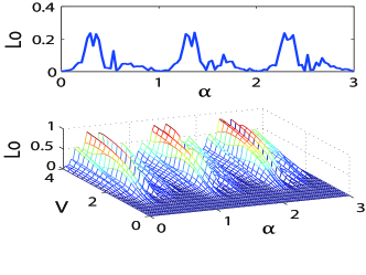
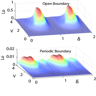
Fig.1 displays the average inverse participation ratio as a function of and (lower panel). To show clearly the dependence of on , we present the versus with a fixed in the upper panel. We find that arrives at its maximum at about (integer+). As is increased, the system becomes more dynamically localized at the edge sites. is a periodic function of and with periods 1 and , respectively. This is a reflection of symmetry in the Hamiltonian, i.e., the Hamiltonian remains unchanged by substitution, , From Fig. 1 we can also observe that is very close to zero at and where is an integer. This can be explained as a direct consequence of the space-independent on-site potential, and
Fig.2 shows the AIPR as a function of and . As changes, may have one peak or many peaks within one period of , each peak corresponds to an eigenstate well localized at the edge site 1.
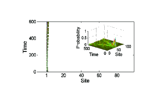
The observed dynamical localization quantified by AIPR depends on the initial state of the system, for example, the system is well dynamically localized with the excitation being initially at site 1, while it is extended with the central site being occupied, see Fig. 3. Further numerical results show that is sharply suppressed when the sites other than site 1 are occupied initially.
To understand the physics behind the dynamical localization, we calculate the largest probability of finding the system at site 1 when the system is in one of its eigenstates. This calculation would show the overlap between the site 1 and the eigenstate which exhibits largest probability to occupy site 1. The results are given in Fig. 4. Comparing Fig. 1, Fig. 2 and Fig. 4, we find that the and reach their respective maximum and minimum at almost the same and . The dependence of and on manifests the same feature, i.e., they increase as increases.
To shed light on the effect of boundary, we now turn to discuss the situation with a periodic boundary condition. The A-A model in this situation can be solved analytically as follows. Suppose that the n-th eigenstate of the Hamiltonian restricted to a single particle in the 1D lattice is given by , the eigenvalue equation leads to the Harper equation,
| (5) | |||||
We shall consider the commensurate potential with a rational given by with and being integers which are prime to each other. Since the potential is periodic with a period , the wave functions take the Bloch form, , for the lattice with the periodic boundary condition. Omitting the eigenstate index where not confused and taking for , we have , Eq. (5) then follows
| (6) | |||||
To be specific, we take , then and . By , Eq. (6) reduces to,
| (7) |
where
| (11) |
and . Solving the eigenvalue equation (7), we can obtain three eigenvalues for a given ,
| (13) |
where The corresponding three eigenstates are,
| (17) |
where
| (18) |
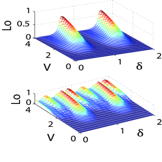
Collecting these equations, we calculate the AIPR and exhibit the results in Fig. 6 (bottom panel). The AIPR under the periodic condition is very small, by contrast, the open boundary condition helps dynamical localization, as the top panel of Fig. 6 shows. This again can be explained as a consequence of small overlap between the site 1 and the eigenstates of the system. In fact, under the periodic condition, all eigenstates of the system are extended, this is enforced by the Bloch theorem.
The time evolution of an isolated macroscopic quantum system initially prepared in an out-of-equilibrium state is currently turning from an abstract concept to a real phenomenon that can be observed and studied experimentally. This striking change has been mainly driven by experiments on cold atomsbloch08 ; polkovnikov11 , but it will be surely given further impulse in the near future by the fast progresses in time-resolved spectroscopy on condensed-matter systems.
IV off-diagonal A-A model
Now we extend the study to the the generalized 1D A-A model, which is described by the following Hamiltonian,
| (19) | |||||
This Hamiltonian is different from the model in Eq. (1) at the inhomogeneity in hopping strength described by cosine modulations. The modulations have the same periodicity as in the on-site potential energy and its amplitude is characterized by . The special case with corresponds to the diagonal A-A model, and the generalized A-A model can be derived starting from an ancestor 2D Hofstadter model with next-nearest-neighbor hopping terms. It has been shown recently sarma13 that the commensurate off-diagonal A-A model is topologically nontrivial in the gapless regime and supports zero-energy edge modes. Unlike the incommensurate case, the nontrivial topology in the off-diagonal A-A model is attributed to the topological properties of the one-dimensional Majorana chain.
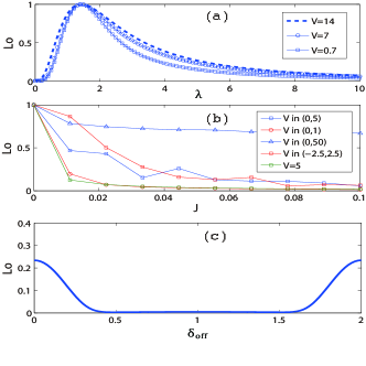
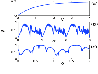
Fig. 6 shows the AIPR as a function of , and with the system initially at site 1. We find that , the modulation amplitude of the on-site potential, does not shift the peak, but the larger the , the bigger the AIPR is (Fig. 6-(a)). Randomness of increases the AIPR, see Fig. 6-(b), which is reminisant of Anderson localization in a disordered medium. The phases and can be tuned independently in experiment, so and can be treated as independent variables. The phase can alter the AIPR, see Fig. 6-(c), the AIPR arrives at a maximum when , and it is very close to 0 when in an interval of .
V Conclusion
To conclude, we have found a signature for the existence of edge states in terms of dynamical feature of the system. A quantity to measure the dynamical localization called average inverse participation ratio (AIPR) is introduced and discussed. We have calculated the AIPR for the diagonal and off-diagonal diaAubry-André model. Our findings suggest that the AIPR can be taken as a measure to quantify the dynamical localization of quantum system, in particular it can be chosen as a witness of edge state. Our strategy is to make use of the definition of edge states and it is applicable for both gapped and gapless systems in one dimension.
This work is supported by the NSF of China under Grants Nos 61078011, 10935010 and 11175032 as well as the National Research Foundation and Ministry of Education, Singapore under academic research grant No. WBS: R-710-000-008-271.
References
- (1) B. A. Bernevig, T. L. Hughes, and S. C. Zhang, Science 314, 1757 (2006).
- (2) L. Fu, C. L. Kane and E. J. Mele, Phys. Rev. Lett. 98, 106803 (2007).
- (3) M. König, S. Wiedmann, C. Brüne, A. Roth, H. Buhmann, L.W. Molenkamp, X.-L. Qi, and S.-C. Zhang, Science 318, 766 (2007).
- (4) D. Hsieh, D. Qian, L. Wray, Y. Xia, Y. Hor, R. J. Cava, and M. Z. Hasan, Nature (London) 452, 970 (2008)
- (5) Y. L. Chen, J. G. Analytis, J.-H. Chu, Z. K. Liu, S. K. Mo, X. L. Qi, H. J. Zhang, D. H. Lu, X. Dai, Z. Fang, S. C. Zhang, I. R. Fisher, Z. Hussain, and Z.-X. Shen, Science 325, 178 (2009).
- (6) Y. Xia, D. Qian, D. Hsieh, L. Wray, A. Pal, H. Lin, A. Bansil, D. Grauer, Y. S. Hor, R. J. Cava, and M. Z. Hasan, Nature Phys. 5, 398 (2009).
- (7) D. Hsieh, Y. Xia, D. Qian, L. Wray, F. Meier, J. H. Dil, J. Osterwalder, L. Patthey, A. V. Fedorov, H. Lin, A. Bansil, D. Grauer, Y. S. Hor, R. J. Cava, and M. Z. Hasan, Phys. Rev. Lett. 103, 146401 (2009).
- (8) K. Kuroda et al, Phys. Rev. Lett. 108, 206803 (2012).
- (9) N. Y. Yao, A. V. Gorshkov, C. R. Laumann, A. M. Läuchli, J. Ye, and M. D. Lukin, Phys. Rev. Lett. 110, 185302 (2013).
- (10) C. Nayak, S. H. Simon, A. Stern, M. Freedman, and S. Das Sarma, Rev. Mod. Phys. 80, 1083 (2008).
- (11) J. E. Moore, Nature (London) 464, 194 (2010).
- (12) S. Aubry and G. Andr‘e, Ann. Israel Phys. Soc. 3, 133 (1980).
- (13) L. Fallani, J. E. Lye, V. Guarrera, C. Fort, and M. Inguscio, Phys. Rev. Lett. 98, 130404 (2007).
- (14) G. Roati, C. D Errico, L. Fallani, M. Fattori, C. Fort, M. Zaccanti, G. Modugno, M. Modugno and, M. Inguscio, Nature 453, 895 (2008).
- (15) B. Deissler et al., Nat. Phys. 6, 354 (2010).
- (16) P. G. Harper, Proceedings of the Physical Society. Section A 68, 874 (1955).
- (17) D. R. Hofstadter, Phys. Rev. B 14, 2239 (1976).
- (18) J. Billy, V. Josse, Z. Zuo, A. Bernard, B. Hambrecht, P. Lugan, D. Cl ement, L. Sanchez-Palencia, P. Bouyer and, A. Aspect, Nature 453, 891 (2008).
- (19) P. W. Anderson, Phys. Rev. 109, 1492 (1958).
- (20) Y. Avron, R. Seiler, and B. Shapiro, Nucl. Phys. B 265, 364 (1986).
- (21) Li-Jun Lang, Xiaoming Cai, Shu Chen, Phys. Rev. Lett. 108, 220401 (2012).
- (22) I. Bloch, J. Dalibard, and W. Zwerger, Rev. Mod. Phys. 80, 885 (2008).
- (23) A. Polkovnikov, K. Sengupta, A. Silva, and M. Vengalattore, Rev. Mod. Phys. 83, 863 (2011).
- (24) S. Ganeshan, K. Sun, and S. Das Sarma, Phys. Rev. Lett. 110, 180403(2013).