Self-dual soliton solutions in a Chern-Simons-CP(1) model
with a nonstandard kinetic term

Abstract

A generalization of the Chern-Simons-CP(1) model is considered by introducing a nonstandard kinetic term. For a particular case, of this nonstandard kinetic term, we show that the model support self-dual Bogomol’nyi equations. The BPS energy has a bound proportional to the sum of the magnetic flux and the CP(1) topological charge. The self-dual equations are solved analytically and verified numerically.

I Introduction

The $CP(n)$ sigma model have been investigated in detail since the early 70’s mainly as toy models to explore the strong coupling effects of $QCD$ and as effective models of some condensed matter systems gral -gral2 .

An important issue related to this type of models concern the existence of soliton type solutions. For the simplest $CP(1)$ mode topological solutions have been shown to existpolyakov . Nevertheless, the solutions are of arbitrary size due to scale invariance. As argued originally by Dzyaloshinsky, Polyakov and Wiegmannpolyakov1 a Chern-Simons term can naturally arise in this type of models and the presence of a dimensional parameter could play some role stabilizing the soliton solutions. A first detailed consideration of this problem was done in Ref.voru where a perturbative analysis around the scale invariant solutions (i.e no Chern Simons coupling $\kappa=0$) showed that the solutions were pushed to infinite size. The problem of the stabilizing topological soliton of the pure $CP(1)$ model by including a Chern-Simons and Maxwell term for the gauge field, was done by nonperturbative analysis in Ref.z ; ta ; tay ; ls ; ls1 ; ls2 . Although, these works showed the possibility of stabilizing the $CP(1)$ sigma model solitons, they do not present self-duality Bogomol’nyi equations. This lack of self-duality can present itself as a disadvantage, at least technically. One reason is that self-dual vortices, such as, for example, those of the Abelian Higgs model SW do not interact by virtue of the stress tensor vanishing identically, and hence multivortex configurations arbitrarily distributed on the plane can be studied systematically.

In the recent years, theories with nonstandard kinetic term, named $k$-field models, have received much attention. The $k$-field models are mainly in connection with effective cosmological modelsAPDM -APDM6 as well as the tachyon matter12 , the ghost condensates 13 -13d and dark matterAPL . The addition of non-linear terms to the kinetic part of the Lagrangian has interesting consequences for topological defects, making it possible for defects to arise without a symmetry-breaking potential term sy . In this context several studies have been conducted, showing that the $k$-theories can support topological soliton solutions both in models of matter as in gauged modelsBAi -BAi4 , SG -SG4 , LS LS1 . These solitons have certain features such as their characteristic size, which are not necessarily those of the standard modelsB -B2

In this article, we investigate a Chern-Simons-$CP(1)$ model with a nonstandard kinetic term. We will show that introducing a particular nonstandard dynamics in a Chern-Simons-$CP(1)$ model, via a function $\omega$ depending on the $CP(1)$ field, we can obtain self-duality Bogomol’nyi equations by minimizing the energy functional of the model. Finally, we will be able to solve the Bogomol’nyi equations and obtain novel analytic expressions for the soliton solutions. This analysis is completed by showing explicitly the principal features of the soliton profiles.

II The theoretical framework

We begin by considering the following $(2+1)$-dimensional Chern-Simons model, coupled to a complex $CP(1)$ field $n(x)$, subject to the constraint $n^{\dagger}n=1$

$$S=S_{cs}+\int d^{3}x\left(\left|D_{\mu}n\right|^{2}-V(n,n^{\dagger})\right)$$ (1)

where $S_{cs}$ is the Chern-Simons action,

$$S_{cs}=\int d^{3}x\frac{\kappa}{4}\epsilon^{\mu\nu\rho}A_{\mu}F_{\nu\rho}$$ (2)

here $F_{\mu\nu}=\partial_{\mu}A_{\nu}-\partial_{\nu}A_{\mu}$, is electromagnetic strength-tensor, $\ D_{\mu}=\partial_{\mu}+iA_{\mu}$ is the covariant derivative. The metric tensor is defined as $g^{\mu\nu}=(1,-1,-1)$. The potential $V(n,n^{\dagger})$ is a function of the field $n(x)$ and its complex conjugate. The constraint can be introduced in the variational process via a Lagrange multiplier. Then, we extremise the following action

$$S=S_{cs}+\int d^{3}x\left(\left|D_{\mu}n\right|^{2}-V(n,n^{\dagger})+\lambda(n^{\dagger}n-1)\right)$$ (3)

The variation of this action yields the field equations,

$$\frac{1}{2}\kappa\epsilon_{\mu\nu\rho}F^{\nu\rho}+J_{\mu}=0$$ (4)

$$D_{\mu}D^{\mu}n+\frac{\partial V}{\partial n^{\dagger}}-\lambda n=0,$$ (5)

where $J_{\mu}=i[(D_{\mu}n)^{\dagger}n-n^{\dagger}D_{\mu}n]$ is the conserved current density and $\lambda=n^{\dagger}\left(D_{\mu}D^{\mu}n+\frac{\partial V}{\partial n^{\dagger}}\right)$, so that

$$D_{\mu}D^{\mu}n+\frac{\partial V}{\partial n^{\dagger}}=\left[n^{\dagger}\left(D_{\mu}D^{\mu}n+\frac{\partial V}{\partial n^{\dagger}}\right)\right]n.$$ (6)

The time component of Eq.(4)

$$\kappa F_{12}=-J_{0}$$ (7)

is Gauss’s law of Chern-Simons dynamics. Integrating it over the entire plane one obtains the important consequence that any object with charge $Q=\displaystyle\int d^{2}xJ_{0}$ also carries magnetic flux $\Phi=\displaystyle\int Bd^{2}x$ Echarge -Echarge2 :

$$\Phi=-\frac{1}{\kappa}Q,$$ (8)

where in the expression of magnetic flux we renamed $F_{12}$ as $B$.

The expression of the energy functional for the static field configuration is

$$E=\int d^{2}x\left(\frac{\kappa^{2}}{4}B^{2}+|D_{i}n|^{2}+V(n,n^{\dagger})\right).$$ (9)

As mentioned in Ref.z ; ta ; tay , the model (1) does not support Bogomol’nyi equations. In fact, as was shown in the Ref.z , it can be established that the energy functional (9) is bounded below by a multiple of the winding number, which is guaranteed to be a non-vanishing energy for non-trivial field configuration. Despite this, it is not possible to saturate the topological bound. This is because the nature of the $CP(1)$ field, which prevents rewrite the expression (9) as sum of square terms plus a topological term. We will consider, here, a generalization of the model (1), which consist on a modification of the model (1) by introducing a nonstandard kinetic term. Specifically, we consider the following $(2+1)$ dimensional model with Chern-Simons-CP(1) Lagrangian

$$S = \int d^{3}x\left(\frac{\kappa}{4}\epsilon^{\mu\nu\rho}A_{\mu}F_{\nu\rho}+\omega(n,n^{\dagger})|D_{0}n|^{2}\right.$$ (10)

$$~{}\ \ \ \ \ \left.\frac{{}}{{}}-|D_{i}n|^{2}+V(n,n^{\dagger})\right)$$

Here, the function $\omega((n,n^{\dagger}))$ is, in principle, an arbitrary function of the $CP(1)$ field.

Since, we are interested on time-independent soliton solutions that ensure the finiteness of the action (10), we are looking for stationary points of the energy which for the static field configuration reads

$$E=\int\,\,d^{2}x\left(\frac{{}}{{}}-\kappa A_{0}B-\omega(n,n^{\dagger})A_{0}^{2}+|D_{i}n|^{2}+V(n,n^{\dagger})\right)$$ (11)

The Gauss law (7) for this system takes the form

$$A_{0}=-\frac{\kappa}{2}\frac{B}{\omega(n,n^{\dagger})}.$$ (12)

Substitution of (12) into (11) leads to

$$E=\int\,\,d^{2}x\left(\frac{\kappa^{2}}{4}\frac{B^{2}}{\omega(n,n^{\dagger})}+|D_{i}n|^{2}+V(n,n^{\dagger})\right)$$ (13)

In order to implement the BPS formalism we first introduce the usual ansatz for describe $CP(1)$ solutions

$$n=\left(\begin{array}[]{c}e^{iN\phi}\cos\frac{\theta}{2}\\ \sin\frac{\theta}{2}\end{array}\right),~{}\theta=\theta\left(r\right),~{}A_{\phi}\left(r\right)=a\left(r\right),$$ (14)

where $N$ is the winding number.

In this ansatz, the magnetic field reads as

$$B=\frac{\left(ra\right)^{\prime}}{r},$$ (15)

the quantity $|D_{i}n|^{2}$ is expressed as

$$\left|D_{i}n\right|^{2}=\left(\frac{\theta^{\prime}}{2}\right)^{2}+\left(a+\frac{N}{r}\right)^{2}\cos^{2}\frac{\theta}{2}+a^{2}\sin^{2}\frac{\theta}{2}.$$

Under this prescription, the energy (13) is expressed as

$$E = \int d^{2}x\left[\frac{\kappa^{2}B^{2}}{4\omega\left(\theta\right)}+V\left(\theta\right)+\left(\frac{\theta^{\prime}}{2}\right)^{2}\right.$$

$$\hskip 28.45274pt\left.+\left(a+\frac{N}{r}\right)^{2}\cos^{2}\frac{\theta}{2}+a^{2}\sin^{2}\frac{\theta}{2}\right].$$

The Ampere’s law reads

$$\frac{\kappa^{2}}{4}\left(\frac{B}{\omega}\right)^{\prime}-\left[a+\frac{N}{2r}\left(1+\cos\theta\right)\right]=0,$$ (17)

and the $\theta-$ field equation is

$$\theta^{\prime\prime}+\frac{\theta^{\prime}}{r}+\frac{\kappa^{2}}{2}\frac{~{}B^{2}}{\omega^{2}}\frac{\partial\omega}{\partial\theta}-2\frac{\partial V}{\partial\theta}+\left(2a+\frac{N}{r}\right)\frac{N}{r}\sin\theta=0.$$ (18)

In the following we apply the BPS formalism, so after some manipulations the energy can be expressed in the following quadratic form

$$E = \int d^{2}x\ \left\{\frac{\kappa^{2}}{4\omega}\left(B\pm\frac{2}{\kappa}\sqrt{\omega V}\right)^{2}\mp\kappa B\sqrt{\frac{V}{\omega}}\right.$$

$$\hskip 28.45274pt+\left[\frac{\theta^{\prime}}{2}\sin\frac{\theta}{2}\pm\left(a+\frac{N}{r}\right)\cos\frac{\theta}{2}\right]^{2}\$$

$$\hskip 28.45274pt\left.+\left(\frac{\theta^{\prime}}{2}\cos\frac{\theta}{2}\mp a\sin\frac{\theta}{2}\right)^{2}\mp\frac{1}{2}\frac{N\sin\theta}{r}\theta^{\prime}\ \right\},$$

it is minimized by imposing

$$B = \mp\frac{2}{\kappa}\sqrt{\omega V},$$ (20)

$$\frac{\theta^{\prime}}{2}\sin\frac{\theta}{2} = \mp\left(a+\frac{N}{r}\right)\cos\frac{\theta}{2},$$ (21)

$$\frac{\theta^{\prime}}{2}\cos\frac{\theta}{2} = \pm a\sin\frac{\theta}{2},$$ (22)

where the upper(lower) signal corresponds to $N>0$ $(N<0)$.

The two last equations can be reduced to one given

$$\theta^{\prime}=\mp\frac{N}{r}\sin\theta,$$ (23)

it will be the first BPS equation.

In order to establish a lower bound for the energy the topological solutions, we choose the function $\omega(\theta)$ as

$$\omega(\theta)=\kappa^{2}V(\theta),$$ (24)

so the BPS equation (20) of our CP(1) model becomes

$$B=\mp 2V\left(\theta\right).$$ (25)

In addition it is interesting to note that the relations (12), (24) and (25), imply

$$A_{0}=\pm\frac{1}{\kappa}$$ (26)

which lead us to a soliton solution without electric charge.

In this way, the BPS energy becomes

$$E_{BPS}=\int d^{2}x\left(\mp B\pm\frac{N}{2}\frac{\left(\cos\theta\right)^{\prime}}{r}\right),$$ (27)

where the first integral is the magnetic flux and the second is the CP(1) topological charge ls . The requirement of well-behaved fields at origin and infinity, provide the following boundary conditions for the fields $\theta\left(r\right)$ and $a\left(r\right):$

$$\theta\left(0\right)=\pi~{},~{}~{}\theta\left(\infty\right)=0,$$ (28)

$$a\left(0\right)=0~{},~{}\ \left(ra\right)\left(\infty\right)=-C_{N}$$ (29)

with $C_{N}>0\left(C_{N}<0\right)$ for $N>0~{}\left(N<0\right)$.

With such boundary conditions allow compute the magnetic flux

$$\Phi=\int\,\,d^{2}xB=-2\pi C_{N}\;,$$ (30)

whereas the BPS energy (27) becomes

$$E_{BPS}=2\pi\left|C_{N}\right|+2\pi\left|N\right|,$$ (31)

By using BPS equations the energy (II) can be written as

$$E_{BPS}=\int d^{2}x~{}\varepsilon_{BPS},$$ (32)

where $\varepsilon_{BPS}$ is the BPS energy density,

$$\ \varepsilon_{BPS}=2V(\theta)+\frac{N^{2}\sin^{2}\theta}{2r^{2}},$$ (33)

it is a positive quantity.

Since the solutions of self-dual equations (23) and (25) should be also solutions of the second order equations of motion (17) and (18) we require that the field $a(r)$ obeys

$$a\left(r\right)=-\frac{N}{2r}\left[1+\cos\theta\left(r\right)\right]\text{. }$$ (34)

This equation allows to compute the magnetic field

$$B=\frac{\left(ar\right)^{\prime}}{r}=\mp\frac{N^{2}}{2r^{2}}\sin^{2}\theta,$$ (35)

which implies an equation for the potential,

$$2V\left(\theta\right)=\frac{N^{2}}{2r^{2}}\sin^{2}\theta$$ (36)

This is similar to the “superpotential equation” found in Ref.Ws1 and Ws2 , which relates the potential with topological terms. In the following we solve the BPS equations for $N>0$. The first BPS equation (23),

$$\theta^{\prime}=-\frac{N}{r}\sin\theta,$$ (37)

is solved explicitly and its solution compatible with the boundary conditions (28) is given by

$$\theta\left(r\right)=\arctan\left(\frac{2\left(\frac{r}{r_{0}}\right)^{N}}{\left(\frac{r}{r_{0}}\right)^{2N}-1}\right).$$ (38)

where $r_{0}$ is a parameter characterizing the effective radius of the topological defect. Then, the equation (34) reads

$$a\left(r\right)=-\frac{N}{r}\frac{\left(\frac{r}{r_{0}}\right)^{2N}}{\left(\frac{r}{r_{0}}\right)^{2N}+1}$$ (39)

It provides the following behavior at $r=0$,

$$a\left(r\right)=-\frac{N}{\left(r_{0}\right)^{2N}}\ r^{2N-1}+...$$ (40)

and for $r\rightarrow\infty$, we get

$$a\left(r\right)=-\frac{N}{r}+N\left(r_{0}\right)^{2N}\frac{1}{r^{2N+1}}+...,$$ (41)

it allows to determine asymptotic constant $C_{N}$,

$$C_{N}=N,$$ (42)

This implies the magnetic flux and BPS energy density are proportional to $N$.

We shown the profiles of the BPS solutions for $r_{0}=5$, and some values of the winding number $N$.

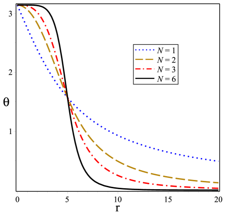
Figure 1: $\theta\left(r\right)$ field profiles.

The Fig. 1 shows the profiles of the $\theta$ field. It is clear that for $N>1$, the asymptotic values is attained rapidly. For larger $N$, the profiles is a rectangle with height $\pi$ and width $r_{0}$.

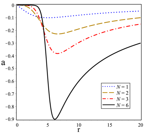
Figure 2: Gauge field $a\left(r\right)$.

The Fig. 2 depicts the profiles of the gauge field, the minimum is located at $r=r_{0}\left(2N-1\right)^{1/2N}$ such that when $N$ increases its position close to the value $r_{0}$. The Fig. 3 shows its asymptotic behavior as explicitly given in Eq. (41).

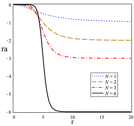
Figure 3: $ra(r)$ profiles.

Fig. 4 depicts the profiles of the magnetic field. For $N=1$ it is a lump centered at origin but for $N>1$ its maximum is located in $r=r_{0}\left(\displaystyle{\frac{N-1}{N+1}}\right)^{1/2N}$. For large values of $N$, it is locate very close to $r_{0}$ and its amplitude goes as $\displaystyle\frac{N^{2}}{2r_{0}^{2}}$.

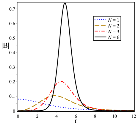
Figure 4: Magnetic field $|B\left(r\right)|$.

Fig. 5 shows the profiles of the BPS energy density which have a similar behavior as the magnetic field.

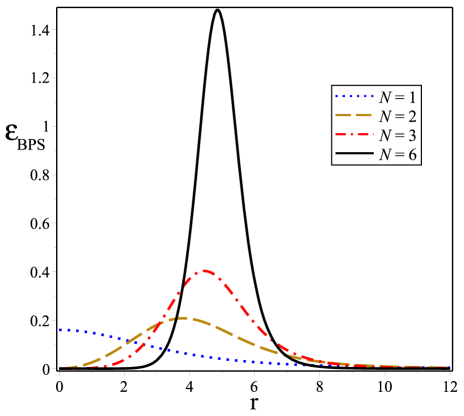
Figure 5: BPS energy density $\varepsilon_{BPS}\left(r\right)$.

III Remarks and conclusions

We have analyzed a Chern-Simons CP(1) model with generalized kinetic term. Such generalization allows to obtain self-duality equations whose analytical solutions minimize the energy density. We have obtained a lower bound for the BPS energy given by a sum of two contributions, the first one is due to the magnetic flux and the second one is related to CP(1) topological charge characterizing the BPS solutions. Because our self–dual solutions provide quantized magnetic flux proportional to $N$, the CP(1) topological charge (see Eqs. (30) and (42)), the BPS energy result proportional to the CP(1) topological charge.

Acknowledgements

We would like to thank the referee for a careful reading of the paper, as well as for the interesting remarks and comments. RC thanks to CAPES, CNPq and FAPEMA (Brazilian agencies) for partial financial support and LS thank to CAPES for full support.

References

- (1) R. Rajaraman, Solitons and Instantons (section 4.5), Elsevier Science, Amsterdam, 1987
- (2) N. Manton, P. Sutcliffe, Topological Solitons, Cambridge Univesity Press, 2004;
- (3) E. Fradkin, Field Theories of Condensed Matter Systems, Addison Wesley, 1991.
- (4) A.A. Belavin, A.M. Polyakov, JETP Lett. 22, 245 (1975).
- (5) I.E. Dzyaloshiskii, A.M. Polyakov and P.B. Wiegmann, Phys. Lett. A 127, 112 (1988).
- (6) P. Voruganti, Phys. Lett. B 223, 181 (1989).
- (7) B.M.A.G. Piette, D.H. Tchrakian, W.J. Zakrzewski, Phys. Lett. B 339, 95 (1994).
- (8) D. H. Tchrakian and K. Arthur, Phys. Lett. B 352, 327 (1995).
- (9) K. Arthur, D. H. Tchrakian and Y. Yang, Phys. Rev. D 54, 5245 (1996).
- (10) Lucas Sourrouille, Alvaro Caso, Gustavo S Lozano, Modern Physics Letters A 26, 637,(2011), [arXiv:hep-th/1002.4847]
- (11) Lucas Sourrouille, Mod. Phys. Lett. A, Vol. 27, 1250094, (2012), [arXiv:hep-th/1111.3100].
- (12) Lucas Sourrouille, Mod. Phys. Lett. A, Vol. 26, 2523 (2011), [arXiv:hep-th/1104.5045].
- (13) A. Jaffe and C. H. Taubes, Monopoles and Vortices (Birkhauser, Basel, 1980).
- (14) C. Armendariz-Picon, T. Damour and V. Mukhanov, Phys. Lett. B 458, 209 (1999).
- (15) C. Armendariz-Picon, V. Mukhanov, P. J. Steinhardt, Phys.Rev.Lett. 85, 4438 (2000)
- (16) C. Armendariz-Picon, V. Mukhanov, Paul J. Steinhardt, Phys. Rev. D63: 103510 (2001)
- (17) T. Chiba, T. Okabe, M. Yamaguchi, Phys.Rev.D 62: 023511 (2000)
- (18) M. Malquarti, E.J. Copeland, A.R. Liddle, Phys.Rev.D 68: 023512 (2003)
- (19) J.U. Kang, V. Vanchurin, S. Winitzki, Phys.Rev.D 76: 083511 (2007)
- (20) E. Babichev, V. Mukhanov and A. Vikman, J. High Energy Phys. 02, 101 (2008)
- (21) A. Sen, JHEP 0207, 065 (2002).
- (22) N. Arkani-Hamed, H.-C. Cheng, M. A. Luty, S. Mukohyama, JHEP 0405, 074 (2004)
- (23) N. Arkani-Hamed, P. Creminelli, S. Mukohyama, M. Zaldarriaga, JCAP 0404: 001 (2004)
- (24) S. Dubovsky, JCAP 0407: 009 (2004)
- (25) D. Krotov, C. Rebbi, V. Rubakov, V. Zakharov, Phys.Rev. D 71: 045014 (2005)
-
(26)
A. Anisimov, A. Vikman, JCAP 0504: 009 (2005).
- (27) V. Mukhanov and A. Vikman, J. Cosmol. Astropart. Phys. 02, 004 (2006).
- (28) C. Armendariz-Picon and E. A. Lim, J. Cosmol. Astropart. Phys. 08, 007 (2005).
- (29) T. H. R. Skyrme, Proc. Roy. Soc. A262, 233.
- (30) D. Bazeia, E. da Hora, C. dos Santos and R. Menezes, Phys. Rev. D 81, 125014 (2010).
- (31) D. Bazeia, E. da Hora, R. Menezes, H. P. de Oliveira and C. dos Santos, Phys. Rev. D 81, 125016 (2010).
- (32) D. Bazeia, R. Casana, E. da Hora, R. Menezes, Phys. Rev. D 85, 125028 (2012).
- (33) R. Casana, M.M. Ferreira, Jr., E. da Hora, Phys.Rev. D 86 085034 (2012).
-
(34)
E. Babichev, Phys. Rev. D 74, 085004 (2006).
E. Babichev, Phys.Rev.D 77, 065021 (2008). - (35) C. Adam, J. Sanchez-Guillen and A. Wereszczynski, J. Phys. A 40, 13625 (2007). Erratum-ibid. A 42, 089801 (2009).
- (36) C. Adam, N. Grandi, J. Sanchez-Guillen and A. Wereszczynski, J. Phys. A 41, 212004 (2008). Erratum- ibid. A 42, 159801 (2009).
- (37) C. Adam, N. Grandi, P. Klimas, J. Sanchez-Guillen and A. Wereszczynski, J. Phys. A 41, 375401 (2008).
- (38) C. Adam, P. Klimas, J. Sanchez-Guillen and A. Wereszczynski, J. Phys. A 42, 135401 (2009).
- (39) Lucas Sourrouille, Physical Review D 87, 067701 (2013), [arXiv:hep-th/1301.5057]
- (40) Lucas Sourrouille, Physical Review D 86, 085014 (2012), [arXiv:hep-th/1207.7171],
- (41) E. Babichev, Phys. Rev. D 74, 085004 (2006).
- (42) D. Bazeia, L. Losano, R. Menezes and J. C. R. E. Oliveira, Eur. Phys. J. C 51, 953 (2007).
- (43) X. Jin, X. Li. and D. Liu, Classical Quantum Gravity 24, 2773 (2007).
- (44) J. Schonfeld, Nucl. Phys. B 185, 157 (1981)
- (45) S. Deser, R. Jackiw, and S. Templeton, Phys. Rev. Lett. 48, 975 (1982)
- (46) S. Deser, R. Jackiw, and S. Templeton, Ann. Phys.(N.Y.) 140, 372 (1982).
- (47) E. Bogomol’nyi, Sov. J. Nucl. Phys 24, 449 (1976)
- (48) C. Adam, C. Naya, J. Sanchez-Guillen, A. Wereszczynski, Phys.Rev. D 86, 045010 (2012); [arXiv:1205.1532]
- (49) C. Adam, C. Naya, J. Sanchez-Guillen, A. Wereszczynski, JHEP 1303, 012 (2013); [arXiv:1212.2741]