Causal hydrodynamics from kinetic theory by doublet scheme in renormalization-group method

Abstract

We develop a general framework in the renormalization-group (RG) method for extracting a mesoscopic dynamics from an evolution equation by incorporating some excited (fast) modes as additional components to the invariant manifold spanned by zero modes. We call this framework the doublet scheme. The validity of the doublet scheme is first tested and demonstrated by taking the Lorenz model as a simple three-dimensional dynamical system; it is shown that the two-dimensional reduced dynamics on the attractive manifold composed of the would-be zero and a fast modes are successfully obtained in a natural way. We then apply the doublet scheme to construct causal hydrodynamics as a mesoscopic dynamics of kinetic theory, i.e., the Boltzmann equation, in a systematic manner with no ad-hoc assumption. It is found that our equation has the same form as thirteen-moment causal hydrodynamic equation, but the microscopic formulae of the transport coefficients and relaxation times are different. In fact, in contrast to the Grad equation, our equation leads to the same expressions for the transport coefficients as given by the Chapman-Enskog expansion method and suggests novel formulae of the relaxation times expressed in terms of relaxation functions which allow a natural physical interpretation of the relaxation times. Furthermore, our theory nicely gives the explicit forms of the distribution function and the thirteen hydrodynamic variables in terms of the linearized collision operator, which in turn clearly suggest the proper ansatz forms of them to be adopted in the method of moments.

1 Introduction

Dissipative hydrodynamic equation is a powerful means for describing the low-frequency and long-wavelength dynamics of many-body systems, which are close to equilibrium state. A typical equation is the Navier-Stokes equation, whose dynamical variables are five fields consisting of temperature, density, and fluid velocity.

One of the problems inherent in the Navier-Stokes equation is instantaneous propagation of information, i.e., the lack of causality, which is attributed to parabolicity of the equation [1, 2, 3, 4]. Here, the parabolicity is a character of diffusion equations containing first-order (second-order) temporal-derivative (spatial-derivative) terms of dynamical variables. This character plagues a relativistically covariant extension of the Navier-Stokes equation.

In 1949, Grad [5] showed that the lack of causality could be circumvented within the framework of kinetic theory, i.e., the Boltzmann equation by employing a method of moments, where an ad-hoc but seemingly plausible ansatz for the functional forms of the distribution function and the moments leads to a closed system of differential equations as the hydrodynamic equations. In particular, for the thirteen-moment approximation to the functional forms, the resultant equation is similar to the Navier-Stokes equation but respects the causality, because the character of the equation is hyperbolic instead of parabolic, with finite propagation speeds. This thirteen-moment causal equation is called the Grad equation, whose dynamical variables are thirteen fields, i.e., temperature, density, fluid velocity, viscous pressure, and heat flux.

In 1996, Jou and his collaborators [6, 7] called the description by the Grad equation mesoscopic since it occupies an intermediate level between the descriptions by the Navier-Stokes equation and the Boltzmann equation. In fact, the Grad equation has been applied to various kinetic problems, e.g., in plasma and in photon transport [8], whose dynamics often cannot be described by the Navier-Stokes equation since the systems are not close enough to the equilibrium state.

However, it has recently turned out that the dynamics described by the Grad equation is not consistent with the Boltzmann equation in the mesoscopic scales of space and time. In fact, numerical simulations [9] have shown that the solutions to the Grad equation are in disagreement with those to the Boltzmann equation in the mesoscopic regime. Although a lot of efforts have been made to reformulate the method of moments so as to get solutions more faithful to the Boltzmann equation [9], the resultant equations are found to still violate the causality, unfortunately [10, 11, 12]. Although various extensions of Grad’s theory has been proposed [13, 14, 15] so as to circumvent the causality problem, the whole consistency between the resultant equations and the solution of the Boltzmann equation in the mesoscopic regime seems not yet achieved. Thus, it is still a challenge to construct the causal hydrodynamic equation consistent with the Boltzmann equation.

The purpose of this paper is to construct the hydrodynamic equation that respects both the causality and the consistency with the Boltzmann equation in the mesoscopic regime. A natural approach to this end is to solve the Boltzmann equation faithfully in a way valid up to the mesoscopic regime and extract from the solution a simpler equation describing the mesoscopic dynamics of the Boltzmann equation. Here, we note that the faithful solution of the Boltzmann equation should lead to an equation that is free from any ansatz for the functional forms of the distribution function and respects the causality that the underlying microscopic theory possesses.

The problem we are facing is to solve a non-linear differential equation such as the Boltzmann equation in an asymptotic regime and extract an effective action or equation with a simpler form than the original one, which reproduces solutions in the asymptotic regime. This is a reduction of the dynamics, and there are some powerful reduction theories of the dynamics [16]. As a reduction theory, we take the “renormalization-group (RG) method” [17, 18, 19, 20, 21, 22, 23, 24, 25, 26, 27, 28, 29, 30, 31]. The RG method as formulated in Refs. [25, 26, 27, 28, 29, 30, 31] is a powerful tool for reducing evolution equations based on the notion of attractive manifold or invariant manifold [32], which the dynamical variables approach to and after some time are eventually confined in. In fact, the RG method [25, 26, 27, 28, 29, 30, 31] has been applied to reduce kinetic equations to a slower dynamics with fewer degrees of freedom, which is realized on the invariant manifold asymptotically.

Hatta and the authors [30, 31] used the RG method to derive the Navier-Stokes equation from the Boltzmann equation. An essential point in the derivation of the Navier-Stokes equation was to utilize five zero modes of the linearized collision operator, which form the invariant manifold on which hydrodynamics is defined; the would-be constant five zero modes, corresponding to temperature, density, and fluid velocity, acquire the time dependence on the manifold by the RG equation.

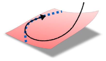
Figure 1: A schematic picture of the invariant/attractive manifold spanned by the zero and excited modes. The solid and dashed lines denote the orbit of an exact solution to the microscopic (Boltzmann) equation, and the asymptotic one on the invariant/attractive manifold spanned only by the zero modes, respectively, while the surface shows the invariant/attractive manifold extended by incorporating excited modes. Under the time evolution of the system, the exact solution starting from a point away from the surface is rapidly attracted along the solid line to the surface, then after performing a fast motion on it, the solution approaches the dashed line, and eventually shows a slow motion confined on it.

Thus, a basic observation presented in the extraction of the mesoscopic dynamics from the Boltzmann equation is to include some excited (fast) modes as additional components of the invariant/attractive manifold, because the mesoscopic dynamics is faster than hydrodynamics that is defined on the invariant manifold spanned by the five zero modes: Figure 1 gives a schematic picture of the invariant/attractive manifold composed of the (would-be) zero and excited modes.

Which excited modes should we adopt? In this paper, we try to determine the excited modes based on the following basic principle in the reduction theory of the dynamics [16]: The resultant dynamics should be as simple as possible because we are interested to reduce the dynamics to a simpler one. Here, we note that this principle is the very spirit of the reduction theory of the dynamics [16], and here the term “simple” is used to express that the resultant dynamics is described with a fewer number of dynamical variables and is given by an equation composed of a fewer number of terms.

We demonstrate that this principle leads to the doublet scheme in the RG method, which uniquely determines the number and form of the excited modes that should be included in the invariant/attractive manifold on which the mesoscopic dynamics of the Boltzmann equation is defined: The doublet scheme can be applied to a wide class of evolution equations. We also demonstrate that the mesoscopic dynamics obtained by the RG equation contains thirteen dynamical variables and respects the causality. We show that the form of the resultant equation is the same as that of the Grad equation, but the microscopic formulae of the coefficients, e.g., the transport coefficients and relaxation times, are different, and our theory leads to the same expressions for the transport coefficients as given by the Chapman-Enskog method [33] and also novel formulae of the relaxation times in terms of relaxation functions, which allow a natural physical interpretation of the relaxation times. Moreover, the distribution function and the moments which are explicitly constructed in our theory provide a proper new ansatz for the functional forms of the distribution function and the moments in the method of moments proposed by Grad.

We here remark that some results in the present paper have been announced in the proceedings [34] by the present authors. In the present paper, we shall make a detailed and complete account on the derivations of the causal hydrodynamic equations together with those of the microscopic expressions of the transport coefficients and relaxation times.

This paper is organized as follows: In Sec. 2, we describe the doublet scheme in the RG method. In Sec. 3, we analyze the Lorenz model [35] in the doublet scheme and demonstrate the validity of the doublet scheme as a method for constructing the invariant/attractive manifold that incorporates the excited modes as well as the would-be zero modes.

In Sec. 4, we give a brief but self-contained account of the Boltzmann equation and Grad’s thirteen-moment approximation in the method of moments. In Sec. 5, we present the causal hydrodynamic equation and the microscopic representations of the transport coefficients and relaxation times that are obtained with the doublet scheme in the RG method. The last section is devoted to a summary and concluding remarks. In A, we give some formulae used for the construction of the doublet scheme. In B, we prove that the mesoscopic dynamics obtained by the doublet scheme is reduced to the slow dynamics described solely by the zero modes in the asymptotic regime after a time. In C, we present the detailed derivation of the causal hydrodynamics as the mesoscopic dynamics of the Boltzmann equation.

2 Derivation of mesoscopic dynamics from generic evolution equation with doublet scheme in RG method

In this section, we develop a method on the basis of the RG method to extract the mesoscopic dynamics from a generic evolution equation by constructing the invariant/attractive manifold incorporating some appropriate excited modes as well as the zero modes of its linearized evolution operator based on the following general principle of the reduction theory of the dynamics [16]: The resultant dynamics should be as simple as possible because we are interested in reducing the dynamics to a simpler one. As mentioned in Sec. 1, we use this principle to derive an equation describing the mesoscopic dynamics, where the number of dynamical variables and terms are reduced as few as possible. We will see that this principle uniquely determines the number and form of the excited modes that should be included in the invariant/attractive manifold on which the mesoscopic dynamics of the evolution equation is defined.

2.1 Evolution equation

As a generic evolution equation, we treat a system of differential equations with two non-linear terms, which represent the relaxation to a static solution and weak perturbation, respectively. The equation reads

$$\frac{\partial}{\partial t}X_{i}=G_{i}(X_{1},\,\cdots,\,X_{N})+\epsilon\,F_{i}(X_{1},\,\cdots,\,X_{N}),\,\,\,\,\,\,i=1,\,\cdots,\,N,$$ (1)

which is also rewritten in a more convenient vector form

$$\frac{\partial}{\partial t}\mbox{\boldmath$X$}=\mbox{\boldmath$G$}(\mbox{\boldmath$X$})+\epsilon\,\mbox{\boldmath$F$}(\mbox{\boldmath$X$}).$$ (2)

In Eq. (2), the dynamical variables are represented by $N$-component vector $X$ ($1<N\leq\infty$), whereas $\mbox{\boldmath$G$}(\mbox{\boldmath$X$})$ and $\mbox{\boldmath$F$}(\mbox{\boldmath$X$})$ are non-linear functions of $X$, and $\epsilon$ is introduced as an indicator of the smallness of $\mbox{\boldmath$F$}(\mbox{\boldmath$X$})$ that is finally set equal to $1$; the vector $\mbox{\boldmath$X$}(t)$ governed by Eq. (2) without $\mbox{\boldmath$F$}(\mbox{\boldmath$X$})$ relaxes to the static solution $\mbox{\boldmath$X$}^{\mathrm{eq}}$ under time evolution as

$$\mbox{\boldmath$X$}(t\rightarrow\infty)\rightarrow\mbox{\boldmath$X$}^{\mathrm{eq}},$$ (3)

which is given as a solution to

$$\mbox{\boldmath$G$}(\mbox{\boldmath$X$}^{\mathrm{eq}})=0.$$ (4)

Here, we suppose that the static solution $\mbox{\boldmath$X$}^{\mathrm{eq}}$ is unique and forms a well-defined $M_{0}$-dimensional invariant manifold with $M_{0}$ being smaller than or equal to $N$. This means that $\mbox{\boldmath$X$}^{\mathrm{eq}}$ is parametrized by $M_{0}$ integral constants $C_{\alpha}$ with $\alpha=1,\,\cdots,\,M_{0}$;

$$\mbox{\boldmath$X$}^{\mathrm{eq}}=\mbox{\boldmath$X$}^{\mathrm{eq}}(C_{1},\,\cdots,\,C_{M_{0}}).$$ (5)

We first define the linearized evolution operator $A$ by

$$A_{ij}\equiv\frac{\partial}{\partial X_{j}}G_{i}(X_{1},\,\cdots,\,X_{N})\Bigg{|}_{\mbox{\boldmath$X$}=\mbox{\boldmath$X$}^{\mathrm{eq}}}.$$ (6)

We note that in accordance with Eq. (5), $A$ has $M_{0}$ eigenvectors belonging to the zero eigenvalue, i.e., zero modes, and the dimension of the kernel of $A$ is $M_{0}$; i.e., dim $[\textrm{ker}\,A]=M_{0}$. In fact, by differentiating Eq. (4) with respect to the $M_{0}$ integral constants $C_{\alpha}$, we have

$$A\,\partial\mbox{\boldmath$X$}^{\mathrm{eq}}/\partial C_{\alpha}=0,$$ (7)

which means that $\mbox{\boldmath$\varphi$}^{\alpha}_{0}$ defined by

$$\mbox{\boldmath$\varphi$}^{\alpha}_{0}=\partial\mbox{\boldmath$X$}^{\mathrm{eq}}/\partial C_{\alpha},$$ (8)

are the $M_{0}$ zero modes. The invariant manifold is spanned by $\mbox{\boldmath$\varphi$}^{\alpha}_{0}$ with $\alpha=1,\,\cdots,\,M_{0}$.

We define the projection operator $P_{0}$ onto the kernel of $A$, which is called the P₀ space, and the projection operator $Q_{0}$ onto the Q₀ space as the complement to the P₀ space: With the use of an inner product which satisfies the positive definiteness of the norm as $\langle\,\mbox{\boldmath$\psi$}\,,\,\mbox{\boldmath$\psi$}\,\rangle>0$ with $\mbox{\boldmath$\psi$}\neq 0$, we define

$$P_{0}\,\mbox{\boldmath$\psi$}\equiv\sum_{\alpha,\beta=1}^{M_{0}}\,\mbox{\boldmath$\varphi$}^{\alpha}_{0}\,\eta^{-1}_{0\alpha\beta}\,\langle\,\mbox{\boldmath$\varphi$}^{\beta}_{0}\,,\,\mbox{\boldmath$\psi$}\,\rangle,\,\,\,Q_{0}\equiv 1-P_{0},$$ (9)

where $\eta^{-1}_{0\alpha\beta}$ is the inverse matrix of the P₀-space metric matrix $\eta^{\alpha\beta}_{0}$ defined by

$$\eta^{\alpha\beta}_{0}\equiv\langle\,\mbox{\boldmath$\varphi$}^{\alpha}_{0}\,,\,\mbox{\boldmath$\varphi$}^{\beta}_{0}\,\rangle.$$ (10)

It is easily verified that the following identity is satisfied:

$$\langle\,\mbox{\boldmath$\varphi$}^{\alpha}_{0}\,,\,P_{0}\,\mbox{\boldmath$\psi$}\,\rangle=\langle\,\mbox{\boldmath$\varphi$}^{\alpha}_{0}\,,\,\mbox{\boldmath$\psi$}\,\rangle,$$ (11)

with $\psi$ being an arbitrary vector.

We assume that the other eigenvalues of $A$ are real negative and negative eigenvalues closest to zero are discrete. Accordingly we suppose that with the inner product $A$ is self-adjoint,

$$\langle\,A\,\mbox{\boldmath$\psi$}\,,\,\mbox{\boldmath$\chi$}\,\rangle=\langle\,\mbox{\boldmath$\psi$}\,,\,A\,\mbox{\boldmath$\chi$}\,\rangle,$$ (12)

where $\psi$ and $\chi$ are arbitrary vectors. We will see that this self-adjoint nature of $A$ plays an essential role in making the form of the resultant equation simpler.

2.2 Approximate solution around arbitrary initial time

To obtain the mesoscopic dynamics of Eq. (2), first we apply the perturbation theory to construct a solution to Eq. (2), which represents the motion caused by the zero modes and the excited modes. Let $\mbox{\boldmath$X$}(t)$ be an yet unknown exact solution to Eq. (2) with an initial condition given at, say, $t=-\infty$: The solution forms an orbit $\mbox{\boldmath$X$}(t)$ parametrized by $t$. Then let us pick up an arbitrary point $\mbox{\boldmath$X$}(t_{0})$ on the orbit. In accordance with the general formulation of the RG method [25, 26, 28, 29], we try to construct a perturbative solution $\mbox{\boldmath$\tilde{X}$}(t\,;\,t_{0})$ with the initial value set to $\mbox{\boldmath$X$}(t_{0})$ at $t=t_{0}$:

$$\mbox{\boldmath$\tilde{X}$}(t=t_{0}\,;\,t_{0})=\mbox{\boldmath$X$}(t_{0}).$$ (13)

Here, we have made explicit the $t_{0}$ dependence of $\mbox{\boldmath$\tilde{X}$}(t=t_{0}\,;\,t_{0})$. It is noted that in the RG method the initial value $\mbox{\boldmath$X$}(t_{0})$ and the RG equation applied to the perturbative solution $\mbox{\boldmath$\tilde{X}$}(t\,;\,t_{0})$ provide the invariant/attractive manifold and the reduced dynamics defined on it, respectively.

The initial value as well as the perturbative solution are expanded with respect to $\epsilon$ as follows:

$$\mbox{\boldmath$\tilde{X}$}(t\,;\,t_{0}) = \mbox{\boldmath$\tilde{X}$}_{0}(t\,;\,t_{0})+\epsilon\,\mbox{\boldmath$\tilde{X}$}_{1}(t\,;\,t_{0})+\epsilon^{2}\,\mbox{\boldmath$\tilde{X}$}_{2}(t\,;\,t_{0})+\cdots,$$ (14)

$$\mbox{\boldmath$X$}(t_{0}) = \mbox{\boldmath$X$}_{0}(t_{0})+\epsilon\,\mbox{\boldmath$X$}_{1}(t_{0})+\epsilon^{2}\,\mbox{\boldmath$X$}_{2}(t_{0})+\cdots.$$ (15)

The respective initial conditions at $t=t_{0}$ are set up as

$$\mbox{\boldmath$\tilde{X}$}_{l}(t=t_{0}\,;\,t_{0})=\mbox{\boldmath$X$}_{l}(t_{0}),\,\,\,\,\,\,l=0,\,1,\,2,\,\cdots.$$ (16)

In the expansion, the zeroth-order initial value $\mbox{\boldmath$\tilde{X}$}_{0}(t_{0}\,;\,t_{0})=\mbox{\boldmath$X$}_{0}(t_{0})$ is supposed to be as close as possible to the exact solution.

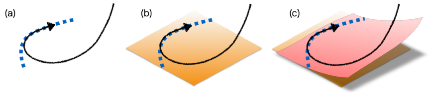
Figure 2: A geometrical illustration of the perturbative construction of the invariant/attractive manifold for the mesoscopic dynamics. In all the panels, the solid lines denote the orbit of an exact solution to the generic evolution equation (2), while the dashed ones represent the asymptotic one confined on the manifold spanned by the zero modes, which can be identified by the zeroth-order analysis; this manifold is represented as a surface presented in panel (b). The new surface shown in panel (c) represents the manifold modified (extended) by incorporating some excited modes properly so as to a closed dynamics is obtained up to the second-order of the perturbation, which is identified with the mesoscopic dynamics.

Substituting the above expansions into Eq. (2), we obtain the series of the perturbative equations with respect to $\epsilon$. Now we are interested in the slow behavior of the solution in the asymptotic regime, and we suppose that the zeroth-order solution is given by a static solution spanned by the zero modes; excited modes and the slippery behavior of the zero modes (as given by secular terms) are to be incorporated in the first- and higher-order solutions. Here, we carry out the perturbative analysis up to the second order, which is necessary to obtain the mesoscopic dynamics.

Before entering the perturbative analysis, we illustrate in a geometrical way in Fig. 2 the way how the invariant/attractive manifold spanned solely by the zero modes is extended or improved so as to accommodate whole the mesoscopic dynamics.

The zeroth-order equation reads

$$\frac{\partial}{\partial t}\mbox{\boldmath$\tilde{X}$}_{0}(t\,;\,t_{0})=\mbox{\boldmath$G$}(\mbox{\boldmath$\tilde{X}$}_{0}(t\,;\,t_{0})).$$ (17)

As mentioned above, we are interested in the slow motion that would be realized asymptotically as $t\rightarrow\infty$. Thus we try to find a stationary solution satisfying

$$\frac{\partial}{\partial t}\mbox{\boldmath$\tilde{X}$}_{0}(t\,;\,t_{0})=0,$$ (18)

which is realized when $\mbox{\boldmath$\tilde{X}$}_{0}(t\,;\,t_{0})$ is the fixed point,

$$\mbox{\boldmath$G$}(\mbox{\boldmath$\tilde{X}$}_{0}(t\,;\,t_{0}))=0.$$ (19)

This is nothing but Eq. (4), and thus $\mbox{\boldmath$\tilde{X}$}_{0}(t\,;\,t_{0})$ is identified with $\mbox{\boldmath$X$}^{\mathrm{eq}}$ because of the uniqueness of the static solution or fixed point which we have assumed:

$$\mbox{\boldmath$\tilde{X}$}_{0}(t\,;\,t_{0})=\mbox{\boldmath$X$}^{\mathrm{eq}}(t_{0}),$$ (20)

accordingly

$$\mbox{\boldmath$X$}_{0}(t_{0})=\mbox{\boldmath$\tilde{X}$}_{0}(t=t_{0}\,;\,t_{0})=\mbox{\boldmath$X$}^{\mathrm{eq}}(t_{0}).$$ (21)

We note that $\mbox{\boldmath$X$}^{\mathrm{eq}}(t_{0})$ depends on $t_{0}$ through the would-be $M_{0}$ integral constants $C_{\alpha}(t_{0})$ with $\alpha=1,\,\cdots,\,M_{0}$ defined in Eq. (5);

$$\mbox{\boldmath$X$}^{\mathrm{eq}}(t_{0})=\mbox{\boldmath$X$}^{\mathrm{eq}}(C_{1}(t_{0}),\,\cdots,\,C_{M_{0}}(t_{0})).$$ (22)

In the following, we suppress the initial time $t_{0}$ when no misunderstanding is expected.

2.3 First-order solution and doublet scheme

The first-order equation reads

$$\frac{\partial}{\partial t}\mbox{\boldmath$\tilde{X}$}_{1}(t)=A\,\mbox{\boldmath$\tilde{X}$}_{1}(t)+\mbox{\boldmath$F$}_{0},$$ (23)

where the inhomogeneous term $\mbox{\boldmath$F$}_{0}$ is defined as

$$\mbox{\boldmath$F$}_{0}\equiv\mbox{\boldmath$F$}(\mbox{\boldmath$X$}^{\mathrm{eq}}).$$ (24)

With the use of the projection operators $P_{0}$ and $Q_{0}$, we can obtain a general solution to Eq. (23) as

$$\mbox{\boldmath$\tilde{X}$}_{1}(t\,;\,t_{0})=\mathrm{e}^{A(t-t_{0})}\,\mbox{\boldmath$\phi$}+(t-t_{0})\,P_{0}\,\mbox{\boldmath$F$}_{0}+(\mathrm{e}^{A(t-t_{0})}-1)\,A^{-1}\,Q_{0}\,\mbox{\boldmath$F$}_{0},$$ (25)

with

$$\mbox{\boldmath$X$}_{1}(t_{0})=\mbox{\boldmath$\tilde{X}$}_{1}(t=t_{0}\,;\,t_{0})=\mbox{\boldmath$\phi$},$$ (26)

where $\phi$ is the integral constant. Without loss of generality, we can suppose that $\phi$ contains no zero modes because such zero modes can be eliminated by the redefinition of the zeroth-order initial value $\mbox{\boldmath$X$}^{\mathrm{eq}}$. We note the appearance of the secular term proportional to $t-t_{0}$ in Eq. (25), which apparently invalidate the perturbative solution when $|t-t_{0}|$ becomes large.

For later convenience, let us expand $\mathrm{e}^{A(t-t_{0})}$ with respect to $t-t_{0}$ and retain the terms up to the first order as

$$\mbox{\boldmath$\tilde{X}$}_{1}(t\,;\,t_{0})=\mbox{\boldmath$\phi$}+(t-t_{0})\,(A\,\mbox{\boldmath$\phi$}+P_{0}\,\mbox{\boldmath$F$}_{0}+Q_{0}\,\mbox{\boldmath$F$}_{0}).$$ (27)

Here, the neglected terms of $O((t-t_{0})^{2})$ are irrelevant when we impose the RG equation, which can be identified with the envelope equation [25] and thus the globally improved solution is constructed by patching the tangent line of the perturbative solution at the arbitrary initial time $t-t_{0}$.

Now the problem is how to extend the vector space beyond that spanned by the zero modes to accommodate the excited modes that are responsible for the closed mesoscopic dynamics; let us call such the closed vector space the P₁ space, which is a subspace of the Q₀ space. The vector fields belonging to the P₁ space constitute the basic variables for the description of the mesoscopic dynamics together with the zero modes. Although it is not apparent a priori whether such a vector space exists, the form of the perturbative solution (27) itself nicely suggests the way how to construct the P₁ space, if we recall that the basic principle of the reduction theory of dynamical systems is to reduce the original equation to a closed system composed of a as small as possible number of variables and equations. In our case, this principle is implemented by requiring that the tangent space of the perturbative solution at $t=t_{0}$ should be spanned by a as small as possible number of independent vectors. In fact the solution (27) is nicely written as a linear combination of the vector $P_{0}\,\mbox{\boldmath$F$}_{0}$ belonging to the P₀ space and the three new vectors, i.e., $\phi$, $A\,\mbox{\boldmath$\phi$}$, and $Q_{0}\,\mbox{\boldmath$F$}_{0}$. Thus, we find that the minimal P₁ space that is closed can be constructed if the following conditions are satisfied:

• $A\,\mbox{\boldmath$\phi$}$ and $Q_{0}\,\mbox{\boldmath$F$}_{0}$ belong to a common vector space.

• The P₁ space is spanned by the bases of the union of $\phi$ and $A\,\mbox{\boldmath$\phi$}$.

The first condition is restated as that $\phi$ and $A^{-1}\,Q_{0}\,\mbox{\boldmath$F$}_{0}$ should belong to a common vector space; note that $\phi$ was defined to be orthogonal to the zero modes of $A$ and hence belong to the Q₀ space.

Thus one sees that the problem is reduced to calculate $A^{-1}\,Q_{0}\,\mbox{\boldmath$F$}_{0}$ and examine whether it is spanned by a finite number of independent vector fields. It is, however, not possible to perform this task for a generic $\mbox{\boldmath$F$}_{0}$. Since our primary purpose is to develop a general theory that is applicable to the reduction of the Boltzmann equation, we here just take the case where $A^{-1}\,Q_{0}\,\mbox{\boldmath$F$}_{0}$ can be expressed in the following form, as in the case for the Boltzmann equation and the Lorenz model,

$$A^{-1}\,Q_{0}\,\mbox{\boldmath$F$}_{0}=\sum_{\mu=1}^{M_{1}}\,(A^{-1}\,\mbox{\boldmath$\varphi$}^{\mu}_{1})\,f_{\mu},$$ (28)

where $f_{\mu}$ with $\mu=1,\,\cdots,\,M_{1}$ are linear independent functions of $\mbox{\boldmath$C$}=(C_{1},\,\cdots,\,C_{M_{0}})$; $f_{\mu}=f_{\mu}(\mbox{\boldmath$C$})$. Here the linear independence of $f_{\mu}$ means that the following statement is satisfied:

$$\sum_{\mu=1}^{M_{1}}\,\alpha^{\mu}\,f_{\mu}(\mbox{\boldmath$C$})=0,\,\,\,\forall\mbox{\boldmath$C$}\Longrightarrow\alpha^{1}=\cdots=\alpha^{M_{1}}=0.$$ (29)

It is noted that $\mbox{\boldmath$\varphi$}^{\mu}_{1}$ can be generic vectors that are not necessarily an eigenvector of $A$. From now on, we shall only consider a generic case where any $\mbox{\boldmath$\varphi$}^{\mu}_{1}$ is not an eigenvector of $A$.

We can take the $M_{1}$ vectors $A^{-1}\,\mbox{\boldmath$\varphi$}^{\mu}_{1}$ as the bases of the vector space spanned by $A^{-1}\,Q_{0}\,\mbox{\boldmath$F$}_{0}$ and $\phi$. Accordingly, $\phi$ can be written as a linear combination of these bases as

$$\mbox{\boldmath$\phi$}=\sum_{\mu=1}^{M_{1}}\,(A^{-1}\,\mbox{\boldmath$\varphi$}^{\mu}_{1})\,C^{\prime}_{\mu}.$$ (30)

Here we have introduced the $M_{1}$ integral constants $C^{\prime}_{\mu}$ as mere coefficients of the basis vectors, which have the $t_{0}$ dependence $C^{\prime}_{\mu}(t_{0})$ as $C_{\alpha}(t_{0})$ does. We stress that the form of $\phi$ given in Eq. (30) is the most general expression that makes $A\,\mbox{\boldmath$\phi$}$ and $Q_{0}\,\mbox{\boldmath$F$}_{0}$ belong to a common space provided that $A^{-1}\,Q_{0}\,\mbox{\boldmath$F$}_{0}$ takes the form given in Eq. (28).

As is clear now, we see that the P₁ space is identified with the vector space spanned by $A^{-1}\,\mbox{\boldmath$\varphi$}^{\mu}_{1}$ and $\mbox{\boldmath$\varphi$}^{\mu}_{1}$ with $\mu=1,\,\cdots,\,M_{1}$. The pair of $A^{-1}\,\mbox{\boldmath$\varphi$}^{\mu}_{1}$ and $\mbox{\boldmath$\varphi$}^{\mu}_{1}$ are called the doublet modes. The Q₀ space is now decomposed into the P₁ space spanned by the doublet modes and the Q₁ space which is the complement to the P₀ and P₁ spaces. The corresponding projection operators are denoted as $P_{1}$ and $Q_{1}$, respectively, whose definitions are given by

$$P_{1}\,\mbox{\boldmath$\psi$} \equiv \sum_{m,n=0,1}\,\sum_{\mu,\nu=1}^{M_{1}}\,A^{-m}\,\mbox{\boldmath$\varphi$}_{1}^{\mu}\,\eta^{-1}_{1m\mu,n\nu}\,\langle\,A^{-n}\,\mbox{\boldmath$\varphi$}^{\nu}_{1}\,,\,\mbox{\boldmath$\psi$}\,\rangle,$$ (31)

$$Q_{1} \equiv Q_{0}-P_{1}.$$ (32)

Here, $\eta^{-1}_{1m\mu,n\nu}$ has been introduced as the inverse matrix of the P₁-space metric matrix given by

$$\eta^{m\mu,n\nu}_{1}\equiv\langle\,A^{-m}\,\mbox{\boldmath$\varphi$}^{\mu}_{1}\,,\,A^{-n}\,\mbox{\boldmath$\varphi$}^{\nu}_{1}\,\rangle.$$ (33)

We note that the direct use of the definitions (31) and (33) leads to the following equalities:

$$\langle\,\mbox{\boldmath$\varphi$}^{\mu}_{1}\,,\,P_{1}\,\mbox{\boldmath$\psi$}\,\rangle=\langle\,\mbox{\boldmath$\varphi$}^{\mu}_{1}\,,\,\mbox{\boldmath$\psi$}\,\rangle,\,\,\,\langle\,A^{-1}\,\mbox{\boldmath$\varphi$}^{\mu}_{1}\,,\,P_{1}\,\mbox{\boldmath$\psi$}\,\rangle=\langle\,A^{-1}\,\mbox{\boldmath$\varphi$}^{\mu}_{1}\,,\,\mbox{\boldmath$\psi$}\,\rangle,$$ (34)

with $\psi$ being an arbitrary vector.

2.4 Second-order solution

The second-order equation is written as

$$\frac{\partial}{\partial t}\mbox{\boldmath$\tilde{X}$}_{2}(t)=A\,\mbox{\boldmath$\tilde{X}$}_{2}(t)+\mbox{\boldmath$K$}(t-t_{0}),$$ (35)

with the time-dependent inhomogeneous term given by

$$\mbox{\boldmath$K$}(t-t_{0})\equiv\frac{1}{2}\,B\,\big{[}\mbox{\boldmath$\tilde{X}$}_{1}(t\,;\,t_{0})\,,\,\mbox{\boldmath$\tilde{X}$}_{1}(t\,;\,t_{0})\big{]}+F_{1}\,\mbox{\boldmath$\tilde{X}$}_{1}(t\,;\,t_{0}).$$ (36)

Here, we have introduced $B$ and $F_{1}$ whose components are given by

$$B_{ijk}\equiv\frac{\partial^{2}}{\partial X_{j}\,\partial X_{k}}G_{i}(X)\Bigg{|}_{\mbox{\boldmath$X$}=\mbox{\boldmath$X$}^{\mathrm{eq}}},\,\,\,F_{1ij}\equiv\frac{\partial}{\partial X_{j}}F_{i}(X)\Bigg{|}_{\mbox{\boldmath$X$}=\mbox{\boldmath$X$}^{\mathrm{eq}}}.$$ (37)

In Eq. (36), we have used the notation

$$(B\,\big{[}\mbox{\boldmath$\psi$}\,,\,\mbox{\boldmath$\chi$}\big{]})_{i}=\sum_{j=1}^{N}\,\sum_{k=1}^{N}\,B_{ijk}\,\psi_{j}\,\chi_{k},$$ (38)

with $\psi_{i}=(\mbox{\boldmath$\psi$})_{i}$ and $\chi_{i}=(\mbox{\boldmath$\chi$})_{i}$.

To obtain appropriate initial values and solutions with the motion coming from the P₀ and P₁ spaces to Eq. (35), we utilize the formulae (176) and (177) given in A: By setting $\mbox{\boldmath$R$}(t-t_{0})=\mbox{\boldmath$K$}(t-t_{0})$ in Eqs. (176) and (177), we find that the initial value and solution to Eq. (35) read

$$\mbox{\boldmath$\tilde{X}$}_{2}(t_{0})=-Q_{1}\,\mathcal{G}(s)\,Q_{0}\,\mbox{\boldmath$K$}(s)\Big{|}_{s=0},$$ (39)

and

$$\mbox{\boldmath$\tilde{X}$}_{2}(t\,;\,t_{0}) = (t-t_{0})\,P_{0}\,\mbox{\boldmath$K$}(0)+(t-t_{0})\,(A-\partial/\partial s)\,P_{1}\,\mathcal{G}(s)\,Q_{0}\,\mbox{\boldmath$K$}(s)\Big{|}_{s=0}$$ (40)

$${}-(1+(t-t_{0})\,\partial/\partial s)\,Q_{1}\,\mathcal{G}(s)\,Q_{0}\,\mbox{\boldmath$K$}(s)\Big{|}_{s=0},$$

respectively. The derivation of this solution is presented in A, where the complete expression of the solution not restricted to $t\sim t_{0}$ is given. In Eq. (40), we have retained only terms up to the first order of $(t-t_{0})$, and introduced a “propagator”

$$\mathcal{G}(s)\equiv(A-\partial/\partial s)^{-1}.$$ (41)

We notice again the appearance of secular terms in Eq. (40).

Summing up the perturbative solutions up to the second order with respect to $\epsilon$, we have the full expression of the initial value and the approximate solution around $t\sim t_{0}$ to the second order:

$$\mbox{\boldmath$X$}(t_{0}) = \mbox{\boldmath$X$}^{\mathrm{eq}}+\epsilon\,\mbox{\boldmath$\phi$}-\epsilon^{2}\,Q_{1}\,\mathcal{G}(s)\,Q_{0}\,\mbox{\boldmath$K$}(s)\Big{|}_{s=0}+O(\epsilon^{3}),$$ (42)

and

$$\mbox{\boldmath$\tilde{X}$}(t\,;\,t_{0}) = \mbox{\boldmath$X$}^{\mathrm{eq}}+\epsilon\,\Bigg{[}\mbox{\boldmath$\phi$}+(t-t_{0})\,A\,\mbox{\boldmath$\phi$}+(t-t_{0})\,P_{0}\,\mbox{\boldmath$F$}_{0}+(t-t_{0})\,Q_{0}\,\mbox{\boldmath$F$}_{0}\Bigg{]}$$ (43)

$${}+\epsilon^{2}\,\Bigg{[}(t-t_{0})\,P_{0}\,\mbox{\boldmath$K$}(0)+(t-t_{0})\,(A-\partial/\partial s)\,P_{1}\,\mathcal{G}(s)\,Q_{0}\,\mbox{\boldmath$K$}(s)\Big{|}_{s=0}$$

$${}-(1+(t-t_{0})\,\partial/\partial s)\,Q_{1}\,\mathcal{G}(s)\,Q_{0}\,\mbox{\boldmath$K$}(s)\Big{|}_{s=0}\Bigg{]}+O(\epsilon^{3}).$$

We note that in Eq. (43) the fast motion caused by the Q₁ space has been eliminated by adopting the appropriate initial value (42).

2.5 RG improvement of perturbative expansion

We emphasize that the solution (43) contains the secular terms that apparently invalidates the perturbative expansion for $t$ away from the initial time $t_{0}$. The point of the RG method lies in the fact that we can utilize the secular terms to obtain a solution valid in a global domain as discussed in Refs. [25, 26, 27, 28, 29, 30, 31]. By applying the RG equation to the local solution (43), we can convert the set of the locally valid approximate solutions to the solution valid in a global domain:

$$\frac{\partial}{\partial t_{0}}\mbox{\boldmath$\tilde{X}$}(t\,;\,t_{0})\Bigg{|}_{t_{0}=t}=0,$$ (44)

which is reduced to

$$\frac{\partial}{\partial t}\mbox{\boldmath$X$}^{\mathrm{eq}}+\epsilon\,\Bigg{[}-A\,\mbox{\boldmath$\phi$}+\frac{\partial}{\partial t}\mbox{\boldmath$\phi$}-P_{0}\,\mbox{\boldmath$F$}_{0}-Q_{0}\,\mbox{\boldmath$F$}_{0}\Bigg{]}$$

$${}+\epsilon^{2}\,\Bigg{[}-P_{0}\,\mbox{\boldmath$K$}(0)-(A-\partial/\partial s)\,P_{1}\,\mathcal{G}(s)\,Q_{0}\,\mbox{\boldmath$K$}(s)\Big{|}_{s=0}$$

$${}+(\partial/\partial s)\,Q_{1}\,\mathcal{G}(s)\,Q_{0}\,\mbox{\boldmath$K$}(s)\Big{|}_{s=0}\Bigg{]}+O(\epsilon^{3})=0.$$ (45)

It is noted that the RG equation (2.5) gives the equation of motion governing the dynamics of the would-be integral constant $C_{\alpha}$ in $\mbox{\boldmath$X$}^{\mathrm{eq}}$ and $C^{\prime}_{\mu}$ in $\phi$. The globally improved solution can be obtained as the initial value (42)

$$\mbox{\boldmath$X$}^{\mathrm{global}}(t) \equiv \mbox{\boldmath$X$}(t_{0}=t)$$ (46)

$$= \mbox{\boldmath$X$}^{\mathrm{eq}}+\epsilon\,\mbox{\boldmath$\phi$}-\epsilon^{2}\,Q_{1}\,\mathcal{G}(s)\,Q_{0}\,\mbox{\boldmath$K$}(s)\Big{|}_{s=0}\Bigg{|}_{t_{0}=t}+O(\epsilon^{3}),$$

where the exact solution to Eq. (2.5) is inserted. It is noteworthy that we have derived the mesoscopic dynamics of Eq. (2) in the form of the pair of Eqs. (2.5) and (46): Equation (46) is nothing but the invariant/attractive manifold of Eq. (2), and Eq. (2.5) describes the mesoscopic dynamics defined on it.

2.6 Reduction of RG equation to simpler form

We find that the RG equation (2.5) includes terms belonging to the Q₁ space that do not constitute the modes responsible for the mesoscopic dynamics. Although these modes could be incorporated as noise terms to make a stochastic mesoscopic dynamics, such an attempt is beyond the scope of the present work. Here we simply average out them to have the mesoscopic dynamics as a regular differential equation. This averaging can be made by taking the inner product of Eq. (2.5) with the zero modes $\mbox{\boldmath$\varphi$}_{0}^{\alpha}$ and the excited modes $A^{-1}\,\mbox{\boldmath$\varphi$}_{1}^{\mu}$ used in the definition of $\phi$.

To this end, we first multiply the projection operators $P_{0}$ and $P_{1}$ from the left-hand side of Eq. (2.5) and we have

$$P_{0}\,\frac{\partial}{\partial t}\mbox{\boldmath$X$}^{\mathrm{eq}}+\epsilon\,\Bigg{[}P_{0}\,\frac{\partial}{\partial t}\mbox{\boldmath$\phi$}-P_{0}\,\mbox{\boldmath$F$}_{0}\Bigg{]}-\epsilon^{2}\,P_{0}\,\mbox{\boldmath$K$}(0)+O(\epsilon^{3})=0,$$ (47)

$$\epsilon\,\Bigg{[}-P_{1}\,A\,\mbox{\boldmath$\phi$}+P_{1}\,\frac{\partial}{\partial t}\mbox{\boldmath$\phi$}-P_{1}\,Q_{0}\,\mbox{\boldmath$F$}_{0}\Bigg{]}$$

$${}-\epsilon^{2}\,P_{1}\,(A-\partial/\partial s)\,P_{1}\,\mathcal{G}(s)\,Q_{0}\,\mbox{\boldmath$K$}(s)\Big{|}_{s=0}+O(\epsilon^{3})=0,$$ (48)

respectively. Here, we have used the fact that $\partial\mbox{\boldmath$X$}^{\mathrm{eq}}/\partial t$ belongs to the P₀ space:

$$\frac{\partial}{\partial t}\mbox{\boldmath$X$}^{\mathrm{eq}}=\sum_{\alpha=1}^{M_{0}}\,\mbox{\boldmath$\varphi$}^{\alpha}_{0}\,\frac{\partial}{\partial t}C_{\alpha},$$ (49)

which is derived from Eqs. (8) and (22).

Then, by taking the inner product of Eqs. (47) and (2.6) with $\mbox{\boldmath$\varphi$}^{\alpha}_{0}$ and $A^{-1}\,\mbox{\boldmath$\varphi$}^{\mu}_{1}$, respectively, we arrive at

$$\langle\,\mbox{\boldmath$\varphi$}^{\alpha}_{0}\,,\,\frac{\partial}{\partial t}(\mbox{\boldmath$X$}^{\mathrm{eq}}+\epsilon\,\mbox{\boldmath$\phi$})\,\rangle-\epsilon\,\langle\,\mbox{\boldmath$\varphi$}^{\alpha}_{0}\,,\,\mbox{\boldmath$F$}_{0}+\epsilon\,F_{1}\,\mbox{\boldmath$\phi$}\,\rangle = \epsilon^{2}\,\frac{1}{2}\,\langle\,\mbox{\boldmath$\varphi$}^{\alpha}_{0}\,,\,B\,\big{[}\mbox{\boldmath$\phi$}\,,\,\mbox{\boldmath$\phi$}\big{]}\,\rangle,$$ (50)

$$\epsilon\,\langle\,A^{-1}\,\mbox{\boldmath$\varphi$}^{\mu}_{1}\,,\,\frac{\partial}{\partial t}\mbox{\boldmath$\phi$}\,\rangle-\epsilon\,\langle\,A^{-1}\,\mbox{\boldmath$\varphi$}^{\mu}_{1}\,,\,\mbox{\boldmath$F$}_{0}+\epsilon\,F_{1}\,\mbox{\boldmath$\phi$}\,\rangle = \epsilon\,\langle\,A^{-1}\,\mbox{\boldmath$\varphi$}^{\mu}_{1}\,,\,A\,\mbox{\boldmath$\phi$}\,\rangle$$ (51)

$${}+\epsilon^{2}\,\frac{1}{2}\,\langle\,A^{-1}\,\mbox{\boldmath$\varphi$}^{\mu}_{1}\,,\,B\,\big{[}\mbox{\boldmath$\phi$}\,,\,\mbox{\boldmath$\phi$}\big{]}\,\rangle,$$

where we have omitted $O(\epsilon^{3})$. In the derivation of Eq. (51), we have used the following identity:

$$\langle\,A^{-1}\,\mbox{\boldmath$\varphi$}^{\mu}_{1}\,,\,(A-\partial/\partial s)\,P_{1}\,\mathcal{G}(s)\,Q_{0}\,\mbox{\boldmath$K$}(s)\Big{|}_{s=0}\,\rangle$$ (52)

$$= \langle\,(A-\partial/\partial s)\,A^{-1}\,\mbox{\boldmath$\varphi$}^{\mu}_{1}\,,\,P_{1}\,\mathcal{G}(s)\,Q_{0}\,\mbox{\boldmath$K$}(s)\Big{|}_{s=0}\,\rangle$$

$$= \langle\,(\mbox{\boldmath$\varphi$}^{\mu}_{1}-A^{-1}\,\mbox{\boldmath$\varphi$}^{\mu}_{1}\,\partial/\partial s)\,,\,P_{1}\,\mathcal{G}(s)\,Q_{0}\,\mbox{\boldmath$K$}(s)\Big{|}_{s=0}\,\rangle$$

$$= \langle\,(\mbox{\boldmath$\varphi$}^{\mu}_{1}-A^{-1}\,\mbox{\boldmath$\varphi$}^{\mu}_{1}\,\partial/\partial s)\,,\,\mathcal{G}(s)\,Q_{0}\,\mbox{\boldmath$K$}(s)\Big{|}_{s=0}\,\rangle$$

$$= \langle\,(A-\partial/\partial s)\,A^{-1}\,\mbox{\boldmath$\varphi$}^{\mu}_{1}\,,\,\mathcal{G}(s)\,Q_{0}\,\mbox{\boldmath$K$}(s)\Big{|}_{s=0}\,\rangle$$

$$= \langle\,A^{-1}\,\mbox{\boldmath$\varphi$}^{\mu}_{1}\,,\,(A-\partial/\partial s)\,\mathcal{G}(s)\,Q_{0}\,\mbox{\boldmath$K$}(s)\Big{|}_{s=0}\,\rangle$$

$$= \langle\,A^{-1}\,\mbox{\boldmath$\varphi$}^{\mu}_{1}\,,\,Q_{0}\,\mbox{\boldmath$K$}(s)\Big{|}_{s=0}\,\rangle$$

$$= \langle\,A^{-1}\,\mbox{\boldmath$\varphi$}^{\mu}_{1}\,,\,\mbox{\boldmath$K$}(0)\,\rangle$$

$$= \frac{1}{2}\,\langle\,A^{-1}\,\mbox{\boldmath$\varphi$}^{\mu}_{1}\,,\,B\,\big{[}\mbox{\boldmath$\phi$}\,,\,\mbox{\boldmath$\phi$}\big{]}\,\rangle+\langle\,A^{-1}\,\mbox{\boldmath$\varphi$}^{\mu}_{1}\,,\,F_{1}\,\mbox{\boldmath$\phi$}\,\rangle.$$

In Eq. (52), we have used the self-adjoint nature of $A$ shown in Eq. (12), the identities given by (34), the definition of $\mathcal{G}(s)$ given by Eq. (41), and the relation derived from Eq. (36); $\mbox{\boldmath$K$}(0)=\frac{1}{2}\,B\,\big{[}\mbox{\boldmath$\phi$}\,,\,\mbox{\boldmath$\phi$}\big{]}+F_{1}\,\mbox{\boldmath$\phi$}$. We note that the pair of Eqs. (50) and (51) is also the equation of motion governing $C_{\alpha}$ in $\mbox{\boldmath$X$}^{\mathrm{eq}}$ and $C^{\prime}_{\mu}$ in $\phi$, which is much simpler than Eq. (2.5).

Two remarks are in order here: (i) The mesoscopic dynamics given by Eqs. (50) and (51) is consistent with the slow dynamics described solely by the zero modes in the asymptotic regime. A proof for this natural property of the mesoscopic dynamics is presented in B. (ii) The doublet scheme in the RG method itself has a universal nature and can be applied to derive a mesoscopic dynamics from a wide class of evolution equations, as far as the equation can be written as Eq. (2) and the linearized evolution operator $A$ is self-adjoint as shown in Eq. (12). Since the Boltzmann equation and the Lorenz model satisfy these conditions as will be seen in C.1 and Sec. 3, respectively, the mesoscopic dynamics of them can be extracted by the doublet scheme. We note that when all the eigenvalues of the linear operator $A$ are real numbers, there exists an inner product with which $A$ can be made self-adjoint. An extension of the doublet scheme to the case where $A$ has complex eigenvalues is left as a future problem.

3 Example: mesoscopic dynamics of the Lorenz model

In this section, we demonstrate how successfully the doublet scheme in the RG method developed in Sec. 2 works to construct the invariant/attractive manifold that incorporates the excited modes as well as the would-be zero modes. To this end, we adopt a simple finite-dimensional dynamical system, i.e., the Lorenz model for thermal convection [35].

The Lorenz model is given by

$$\dot{x} = \sigma(-x+y),$$ (53)

$$\dot{y} = rx-y-xz,$$ (54)

$$\dot{z} = xy-bz,$$ (55)

where $x$, $y$, and $z$ denote the dynamical variables and $\sigma>0$, $r>0$, and $b>0$ are model parameters. For $0<r<1$ there exists one steady state given by

$$(A)\,\,\,\,(x,y,z) = (0,0,0),$$ (56)

while for $1<r$ the steady states are (A) and

$$(B)\,\,\,\,(x,y,z) = (+\sqrt{b(r-1)},+\sqrt{b(r-1)},r-1),$$ (57)

$$(C)\,\,\,\,(x,y,z) = (-\sqrt{b(r-1)},-\sqrt{b(r-1)},r-1).$$ (58)

The linear stability analysis [32] shows that the origin (A) is stable for $0<r<1$ but unstable for $r>1$, while the latter steady states (B) and (C) are stable for $1<r<\sigma(\sigma+b+3)/(\sigma-b-1)\equiv r_{c}$ but unstable for $r>r_{c}$.

In this section, we examine the non-linear stability around the origin (A) for $r\sim 1$. In other words, we are interested in the case where $|r-1|$ is small, say, less than $1$, and hence the amplitudes of the dynamical variables $(x,\,y,\,z)$ are small. Then it is found convenient to rewrite the control parameter $r$ with a small quantity $\epsilon$ as

$$r=1+\chi\epsilon^{2},$$ (59)

with $\chi=\pm 1$ depending on the sign of $r-1$. Furthermore, it turns out that the amplitudes of the dynamical variables scale in the order of $\epsilon$. So we set them as

$$(x,\,y,\,z)=\epsilon\,(X,\,Y,\,Z).$$ (60)

Then the Lorenz model given by Eqs. (53)-(55) is converted into

$$\frac{\mathrm{d}}{\mathrm{d}t}\mbox{\boldmath$X$}=A\,\mbox{\boldmath$X$}+\epsilon\,\left(\begin{array}[]{c}0\\ -X\,Z\\ X\,Y\end{array}\right)+\epsilon^{2}\,\left(\begin{array}[]{c}0\\ \chi\,X\\ 0\end{array}\right),$$ (67)

with $\mbox{\boldmath$X$}\equiv{}^{t}(X,\,Y,\,Z)$ and

$$A \equiv \left(\begin{array}[]{ccc}-\sigma&\sigma&0\\ 1&-1&0\\ 0&0&-b\end{array}\right).$$ (71)

The eigenvalues of $A$ are found to be

$$\lambda_{1}=0,\,\,\,\lambda_{2}=-1-\sigma,\,\,\,\lambda_{3}=-b,$$ (72)

whose respective (right-)eigenvectors are

$$\mbox{\boldmath$U$}_{1}=\left(\begin{array}[]{c}1\\ 1\\ 0\end{array}\right),\,\,\,\mbox{\boldmath$U$}_{2}=\left(\begin{array}[]{c}\sigma\\ -1\\ 0\end{array}\right),\,\,\,\mbox{\boldmath$U$}_{3}=\left(\begin{array}[]{c}0\\ 0\\ 1\end{array}\right).$$ (82)

Since all the eigenvalues are real numbers, it is easily verified that the apparently asymmetric linear operator $A$ is made symmetric with respect to a suitably defined inner product, which can be given with respect to the left-eigenvectors of $A$. Thus, we see that the Lorenz model (67) can be analyzed by the doublet scheme in the RG method developed in the last section where the symmetric property of the linear operator $A$ is assumed and utilized.

We pick up a point $\mbox{\boldmath$X$}(t_{0})$ on an exact solution yet to be determined with some unspecified initial condition, and try to construct a perturbative solution $\tilde{\mbox{\boldmath$X$}}(t;t_{0})$ around $t=t_{0}$ with $\mbox{\boldmath$X$}(t_{0})$ being set up with the initial value. We assume that the initial value i.e., the exact solution and the approximate solution can be expanded with respect to $\epsilon$ as follows: $\mbox{\boldmath$X$}(t_{0})=\mbox{\boldmath$X$}_{0}(t_{0})+\epsilon\,\mbox{\boldmath$X$}_{1}(t_{0})+\epsilon^{2}\,\mbox{\boldmath$X$}_{2}(t_{0})+\cdots$ and $\tilde{\mbox{\boldmath$X$}}(t;t_{0})=\tilde{\mbox{\boldmath$X$}}_{0}(t;t_{0})+\epsilon\,\tilde{\mbox{\boldmath$X$}}_{1}(t;t_{0})+\epsilon^{2}\,\tilde{\mbox{\boldmath$X$}}_{2}(t;t_{0})+\cdots$, which satisfy respective initial conditions $\tilde{\mbox{\boldmath$X$}}_{l}(t=t_{0};t_{0})=\mbox{\boldmath$X$}_{l}(t_{0})$ with $l=0,1,2,\cdots$. Substituting these expansions into Eq. (67), we have a series of perturbative equations.

The zeroth-order equation reads

$$\frac{\mathrm{d}}{\mathrm{d}t}\tilde{\mbox{\boldmath$X$}}_{0}(t;t_{0}) = A\tilde{\mbox{\boldmath$X$}}_{0}(t;t_{0}).$$ (83)

Since we are interested in the asymptotic state as $t\rightarrow\infty$, we take the neutrally stable solution

$$\tilde{\mbox{\boldmath$X$}}_{0}(t;t_{0})=C(t_{0})\mbox{\boldmath$U$}_{1},$$ (84)

where $C(t_{0})$ is an integral constant and we have made it explicit that the solution may depend on the initial time $t_{0}$. We note that $C(t_{0})$ corresponds to $C_{\alpha}(t_{0})$ in the general case discussed in Sec. 2 with $M_{0}=1$. The initial value corresponding to the solution (84) is

$$\mbox{\boldmath$X$}_{0}(t_{0})=\tilde{\mbox{\boldmath$X$}}_{0}(t=t_{0};t_{0})=C(t_{0})\mbox{\boldmath$U$}_{1}.$$ (85)

We note that the P₀ space is spanned by the zero mode $\mbox{\boldmath$U$}_{1}$.

The first-order equation reads

$$\frac{\mathrm{d}}{\mathrm{d}t}\tilde{\mbox{\boldmath$X$}}_{1}(t;t_{0})=A\tilde{\mbox{\boldmath$X$}}_{1}(t;t_{0})+C^{2}(t_{0})\mbox{\boldmath$U$}_{3},$$ (86)

whose general solution may be written as

$$\tilde{\mbox{\boldmath$X$}}_{1}(t;t_{0}) = \mathrm{e}^{L(t-t_{0})}\mbox{\boldmath$X$}_{1}(t_{0})+(\mathrm{e}^{A(t-t_{0})}-1)A^{-1}C^{2}(t_{0})\mbox{\boldmath$U$}_{3}$$ (87)

$$= \mbox{\boldmath$X$}_{1}(t_{0})+(t-t_{0})(A\mbox{\boldmath$X$}_{1}(t_{0})+C^{2}(t_{0})\mbox{\boldmath$U$}_{3})+O((t-t_{0})^{2}).$$

As in the general case discussed in Sec. 2, we specify the initial value $\mbox{\boldmath$X$}_{1}(t_{0})$ so that the dimension of the tangent space given by the term proportional to $t-t_{0}$ of the solution (87) is as small as possible. This requirement is satisfied if $A\mbox{\boldmath$X$}_{1}(t_{0})$ belongs to a space spanned by $\mbox{\boldmath$U$}_{3}$. Thus we set

$$\mbox{\boldmath$X$}_{1}(t_{0})=A^{-1}\mbox{\boldmath$U$}_{3}C^{\prime}(t_{0})=-\frac{1}{b}\mbox{\boldmath$U$}_{3}C^{\prime}(t_{0}).$$ (88)

Here, $C^{\prime}(t_{0})$ is an integral constant corresponding to $C^{\prime}_{\mu}(t_{0})$ in Sec. 2 with $M_{1}=1$. In accordance with the general scheme, the P₁ space is spanned by the doublet modes

$$\mbox{\boldmath$U$}_{3},\,\,\,A^{-1}\mbox{\boldmath$U$}_{3}.$$ (89)

One notice that the doublet modes in the present simple case happen to belong to a common space; recall that $\mbox{\boldmath$U$}_{3}$ is an eigenvector of $A$. Thus, the left vector $\mbox{\boldmath$U$}_{2}$ belongs to the Q₁ space complement to the P₀ and P₁ spaces. The structure of the vector space is summarized as follows:

$$\mathrm{P}_{0}\,\,\, : \,\,\,\mbox{\boldmath$U$}_{1},$$ (90)

$$\mathrm{P}_{1}\,\,\, : \,\,\,\mbox{\boldmath$U$}_{3},$$ (91)

$$\mathrm{Q}_{1}\,\,\, : \,\,\,\mbox{\boldmath$U$}_{2}.$$ (92)

The second-order equation reads

$$\frac{\mathrm{d}}{\mathrm{d}t}\tilde{\mbox{\boldmath$X$}}_{2}(t;t_{0})=A\tilde{\mbox{\boldmath$X$}}_{2}(t;t_{0})+K(t-t_{0})\frac{1}{1+\sigma}(\sigma\mbox{\boldmath$U$}_{1}-\mbox{\boldmath$U$}_{2}),$$ (93)

with the time-dependent inhomogeneous term

$$K(t-t_{0})\equiv\chi C(t_{0})-C(t_{0})\Bigg{[}\frac{C^{2}(t_{0})}{b}(1-\mathrm{e}^{-b(t-t_{0})})-\mathrm{e}^{-b(t-t_{0})}\frac{1}{b}C^{\prime}(t_{0})\Bigg{]}.$$ (94)

A general solution to Eq. (93) is given by

$$\tilde{\mbox{\boldmath$X$}}_{2}(t;t_{0}) = \mathrm{e}^{A(t-t_{0})}\Big{[}\mbox{\boldmath$X$}_{2}(t_{0})+Q_{1}(A-\partial/\partial s)^{-1}Q_{0}K(s)\frac{1}{1+\sigma}(\sigma\mbox{\boldmath$U$}_{1}-\mbox{\boldmath$U$}_{2})\Big{|}_{s=0}\Big{]}$$ (95)

$${}+(1-\mathrm{e}^{(t-t_{0})\partial/\partial s})(-\partial/\partial s)^{-1}P_{0}K(s)\frac{1}{1+\sigma}(\sigma\mbox{\boldmath$U$}_{1}-\mbox{\boldmath$U$}_{2})\Big{|}_{s=0}$$

$${}+(\mathrm{e}^{A(t-t_{0})}-\mathrm{e}^{(t-t_{0})\partial/\partial s})P_{1}(A-\partial/\partial s)^{-1}Q_{0}K(s)\frac{1}{1+\sigma}(\sigma\mbox{\boldmath$U$}_{1}-\mbox{\boldmath$U$}_{2})\Big{|}_{s=0}$$

$${}-\mathrm{e}^{(t-t_{0})\partial/\partial s}Q_{1}(A-\partial/\partial s)^{-1}Q_{0}K(s)\frac{1}{1+\sigma}(\sigma\mbox{\boldmath$U$}_{1}-\mbox{\boldmath$U$}_{2})\Big{|}_{s=0}.$$

We can utilize the initial value $\mbox{\boldmath$X$}_{2}(t_{0})$ to eliminate the unwanted fast motion caused by the Q₁ space as

$$\mbox{\boldmath$X$}_{2}(t_{0})=\tilde{\mbox{\boldmath$X$}}_{2}(t=t_{0};t_{0}) = -Q_{1}(A-\partial/\partial s)^{-1}Q_{0}K(s)\frac{1}{1+\sigma}(\sigma\mbox{\boldmath$U$}_{1}-\mbox{\boldmath$U$}_{2})\Big{|}_{s=0}$$ (96)

$$= -((-1-\sigma)-\partial/\partial s)^{-1}K(s)\Big{|}_{s=0}\frac{1}{1+\sigma}(-\mbox{\boldmath$U$}_{2}),$$

which leads to

$$\tilde{\mbox{\boldmath$X$}}_{2}(t;t_{0}) = (1-\mathrm{e}^{(t-t_{0})\partial/\partial s})(-\partial/\partial s)^{-1}K(s)\Big{|}_{s=0}\frac{1}{1+\sigma}\sigma\mbox{\boldmath$U$}_{1}$$ (97)

$${}-\mathrm{e}^{(t-t_{0})\partial/\partial s}((-1-\sigma)-\partial/\partial s)^{-1}K(s)\Big{|}_{s=0}\frac{1}{1+\sigma}(-\mbox{\boldmath$U$}_{2}).$$

We stop the perturbative analysis in this order.

Summing up the above solutions, the perturbative solutions and initial values are given by

$$\tilde{\mbox{\boldmath$X$}}(t;t_{0}) = C(t_{0})\mbox{\boldmath$U$}_{1}+\epsilon\Bigg{[}\mathrm{e}^{A(t-t_{0})}A^{-1}\mbox{\boldmath$U$}_{3}C^{\prime}(t_{0})+(\mathrm{e}^{A(t-t_{0})}-1)A^{-1}C^{2}(t_{0})\mbox{\boldmath$U$}_{3}\Bigg{]}$$ (98)

$${}+\epsilon^{2}\Bigg{[}(1-\mathrm{e}^{(t-t_{0})\partial/\partial s})(-\partial/\partial s)^{-1}K(s)\Big{|}_{s=0}\frac{1}{1+\sigma}\sigma\mbox{\boldmath$U$}_{1}$$

$${}-\mathrm{e}^{(t-t_{0})\partial/\partial s}((-1-\sigma)-\partial/\partial s)^{-1}K(s)\Big{|}_{s=0}\frac{1}{1+\sigma}(-\mbox{\boldmath$U$}_{2})\Bigg{]},$$

$$\mbox{\boldmath$X$}(t_{0}) = C(t_{0})\mbox{\boldmath$U$}_{1}+\epsilon A^{-1}\mbox{\boldmath$U$}_{3}C^{\prime}(t_{0})$$ (99)

$${}+\epsilon^{2}\Bigg{[}-((-1-\sigma)-\partial/\partial s)^{-1}K(s)\Big{|}_{s=0}\frac{1}{1+\sigma}(-\mbox{\boldmath$U$}_{2})\Bigg{]},$$

respectively. Applying the RG equation $\partial\tilde{\mbox{\boldmath$X$}}(t;t_{0})/\partial t_{0}|_{t_{0}=t}=0$ to Eq. (98), we have

$$\dot{C}\mbox{\boldmath$U$}_{1}+\epsilon\Bigg{[}-\mbox{\boldmath$U$}_{3}C^{\prime}+A^{-1}\mbox{\boldmath$U$}_{3}\dot{C^{\prime}}-C^{2}\mbox{\boldmath$U$}_{3}\Bigg{]}$$

$${}+\epsilon^{2}\Bigg{[}-K(0)\frac{1}{1+\sigma}\sigma\mbox{\boldmath$U$}_{1}-(-\partial/\partial s)((-1-\sigma)-\partial/\partial s)^{-1}K(s)\Big{|}_{s=0}\frac{1}{1+\sigma}(-\mbox{\boldmath$U$}_{2})\Bigg{]}=0.$$

We can read off the P₀ and P₁ components from this expression as

$$\dot{C} = \epsilon^{2}\frac{\sigma}{1+\sigma}(\chi C+CC^{\prime}/b),$$ (101)

$$\dot{C^{\prime}} = -bC^{\prime}-bC^{2}.$$ (102)

With these $C(t)$ and $C^{\prime}(t)$, the globally improved solution defined on the invariant/attractive manifold is given by

$$\mbox{\boldmath$X$}^{\mathrm{global}}(t) \equiv \mbox{\boldmath$X$}(t_{0}=t)$$ (103)

$$= C(t)\mbox{\boldmath$U$}_{1}+\epsilon A^{-1}\mbox{\boldmath$U$}_{3}C^{\prime}(t)$$

$${}+\epsilon^{2}\Bigg{[}-((-1-\sigma)-\partial/\partial s)^{-1}K(s)\Big{|}_{s=0}\frac{1}{1+\sigma}(-\mbox{\boldmath$U$}_{2})\Bigg{]}\Bigg{|}_{t_{0}=t},$$

or in terms of components

$$x = \epsilon C+\epsilon^{3}\frac{\sigma}{1+\sigma}\Bigg{[}-\frac{1}{1+\sigma}(\chi C-C^{3}/b)+\frac{1}{b-(1+\sigma)}\frac{1}{b}C(C^{2}+C^{\prime})\Bigg{]},$$ (104)

$$y = \epsilon C-\epsilon^{3}\frac{1}{1+\sigma}\Bigg{[}-\frac{1}{1+\sigma}(\chi C-C^{3}/b)+\frac{1}{b-(1+\sigma)}\frac{1}{b}C(C^{2}+C^{\prime})\Bigg{]},$$ (105)

$$z = -\epsilon^{2}\frac{1}{b}C^{\prime},$$ (106)

with ${}^{t}(x,\,y,\,z)=\epsilon\,\mbox{\boldmath$X$}^{\mathrm{global}}$. In the derivations of Eqs. (104) and (105), we have used the identity

$$-((-1-\sigma)-\partial/\partial s)^{-1}K(s)=\frac{1}{1+\sigma}(\chi C-C^{3}/b)-\mathrm{e}^{-bs}\frac{1}{b-(1+\sigma)}(C^{2}+C^{\prime})C/b.$$ (107)

To see what has been obtained, let us see a limiting case. From Eq. (102), we identify the relaxation time of $C^{\prime}$ with $1/b$. In fact, after the time evolution from $t=0$ to $t>1/b$, $C^{\prime}$ approaches to

$$C^{\prime}=-C^{2}.$$ (108)

Substituting $C^{\prime}=-C^{2}$ into Eqs. (101), (104)-(106), we obtain a closed equation with respect to $C$ and the invariant manifold parametrized by only $C$. We note that these equations written by $C$ are the same as the reduced equations derived by employing the zero mode from the outset [26]. We stress that the set of Eqs. (101) and (102) governing the dynamics of $C$ and $C^{\prime}$ describes the mesoscopic dynamics of the Lorenz model, and the corresponding two-dimensional invariant/attractive manifold is given by Eqs. (104)-(106). It might be interesting to compare the present result with the previous ones obtained by various reduction theories, e.g., the center manifold theory [32, 36]. This is, however, beyond the scope of this section, whose aim is to show the validity of the doublet scheme in the RG method. Thus, the comparison with the previous works and a further analysis of the Lorenz model by the doublet scheme will be reported elsewhere.

Figure 3: A comparison of the numerical solution of the Lorenz model (the solid line) with the invariant/attractive manifold given by the doublet scheme, i.e., Eqs. (104)-(106) for the parameter set $b=8/3$, $\sigma=10$, $\epsilon=0.5$, and $\chi=+1$ (the surface). The square and cross denote the steady states (fixed points) (A) and (C), respectively, while the big dot with the coordinate $(x,\,y,\,z)=(-0.297,\,-0.212,\,3.437)$ indicates the point from which the solution gets to be confined on the invariant/attractive manifold. The dashed line shows the one-dimensional manifold given by imposing the constraint $C^{\prime}=-C^{2}$.

Figure 4: The time dependence of $x$, $y$, and $z$ with the initial value set at the big dot in Fig. 3 for the same parameter set as that in Fig. 3. The dashed lines denote the numerical solution to the original equation (67), while the solid lines the solution to the reduced equations (101), (102), and (104)-(106). The two solutions are hardly distinguishable.

Let us compare a solution to the Lorenz model (67) with the solution to the reduced equations (101), (102), and (104)-(106) under the same initial condition. For this purpose, we set the parameters of the Lorenz model as $b=8/3$, $\sigma=10$, and $\epsilon=0.5$ and $\chi=+1$, which gives $r=1.25$. In this setting, the origin (A) is unstable, while the steady states (B) and (C) are stable because $1<r<r_{c}\sim 24.7$. In Fig. 3, we present a numerical solution to Eq. (67) whose initial values are $(x,\,y,\,z)=(1,\,5,\,15)$, together with the two-dimensional manifold described by Eqs. (104)-(106) and the one-dimensional manifold that we obtain by imposing the constraint $C^{\prime}=-C^{2}$ on Eqs. (104)-(106). It turns out that the solution is attracted to the two-dimensional manifold at a rather early time, after which the solution remains on it. Then it gets relaxed onto the one-dimensional manifold, and finally comes to the steady state (C) asymptotically. In Fig. 4, we demonstrate the time dependence of $x$, $y$, and $z$ derived by the original equation (67) and that obtained by the reduced equations (101), (102), and (104)-(106). We find that $x(t)$, $y(t)$, and $z(t)$ by Eqs. (101), (102), and (104)-(106) are almost the same as those by Eq. (67). Thus, we conclude that this good agreement ensures the validity of the doublet scheme in the RG method.

4 Basics on Boltzmann equation

In this section, we give the basic notions and a brief summary of the previous works as preliminaries so that the significance of the present work will become clear. First, a brief account is given on the basic properties of the Boltzmann equation with a focus on those of the collision operator. Then, we introduce Grad’s moment method and its thirteen-moment approximation for the functional forms of the distribution function and the moments, and present the explicit form of the Grad equation [5].

4.1 Basic properties of Boltzmann equation

The Boltzmann equation that we consider in the present work reads

$$\frac{\partial}{\partial t}f_{\mbox{\boldmath$v$}}(t,\,\mbox{\boldmath$x$})+\mbox{\boldmath$v$}\cdot\mbox{\boldmath$\nabla$}f_{\mbox{\boldmath$v$}}(t,\,\mbox{\boldmath$x$})=C[f]_{\mbox{\boldmath$v$}}(t,\,\mbox{\boldmath$x$}).$$ (109)

Here, $f_{\mbox{\boldmath$v$}}(t,\,\mbox{\boldmath$x$})$ denotes the distribution function defined in phase space $(\mbox{\boldmath$x$},\,\mbox{\boldmath$v$})$ with $t$ and $\mbox{\boldmath$x$}=(x^{1},\,x^{2},\,x^{3})$ being the space-time coordinate and $\mbox{\boldmath$v$}=(v^{1},\,v^{2},\,v^{3})$ the velocity of the one-shell particle whose mass, momentum, and energy are given as $m$, $m\,\mbox{\boldmath$v$}$, and $m\,|\mbox{\boldmath$v$}|^{2}/2$, respectively. The right-hand side of Eq. (109) is the collision integral,

$$C[f]_{\mbox{\boldmath$v$}}(t,\,\mbox{\boldmath$x$}) \equiv \frac{1}{2!}\,\int_{\mbox{\boldmath$v_{1}$}}\int_{\mbox{\boldmath$v_{2}$}}\int_{\mbox{\boldmath$v_{3}$}}\,\omega(\mbox{\boldmath$v$},\,\mbox{\boldmath$v_{1}$}|\mbox{\boldmath$v_{2}$},\,\mbox{\boldmath$v_{3}$})$$ (110)

$${}\times\,\Big{(}f_{\mbox{\boldmath$v_{2}$}}(t,\,\mbox{\boldmath$x$})\,f_{\mbox{\boldmath$v_{3}$}}(t,\,\mbox{\boldmath$x$})-f_{\mbox{\boldmath$v$}}(t,\,\mbox{\boldmath$x$})\,f_{\mbox{\boldmath$v_{1}$}}(t,\,\mbox{\boldmath$x$})\Big{)},$$

with $\int_{\mbox{\boldmath$v$}}\equiv\int\!\!\mathrm{d}^{3}\mbox{\boldmath$v$}$. Here, $\omega(\mbox{\boldmath$v$},\,\mbox{\boldmath$v_{1}$}|\mbox{\boldmath$v_{2}$},\,\mbox{\boldmath$v_{3}$})$ denotes the transition probability due to the microscopic two particle interaction. We note that $\omega(\mbox{\boldmath$v$},\,\mbox{\boldmath$v_{1}$}|\mbox{\boldmath$v_{2}$},\,\mbox{\boldmath$v_{3}$})$ contains the delta function representing the energy-momentum conservation,

$$\omega(\mbox{\boldmath$v$},\,\mbox{\boldmath$v_{1}$}|\mbox{\boldmath$v_{2}$},\,\mbox{\boldmath$v_{3}$}) \propto \delta^{3}(m\,\mbox{\boldmath$v$}+m\,\mbox{\boldmath$v_{1}$}-m\,\mbox{\boldmath$v_{2}$}-m\,\mbox{\boldmath$v_{3}$})$$ (111)

$${}\times\,\delta(m\,|\mbox{\boldmath$v$}|^{2}/2+m\,|\mbox{\boldmath$v_{1}$}|^{2}/2-m\,|\mbox{\boldmath$v_{2}$}|^{2}/2-m\,|\mbox{\boldmath$v_{3}$}|^{2}/2),$$

and also has the symmetric properties due to the indistinguishability of the particles and the time reversal invariance of the microscopic transition probability,

$$\omega(\mbox{\boldmath$v$},\,\mbox{\boldmath$v_{1}$}|\mbox{\boldmath$v_{2}$},\,\mbox{\boldmath$v_{3}$})=\omega(\mbox{\boldmath$v_{2}$},\,\mbox{\boldmath$v_{3}$}|\mbox{\boldmath$v$},\,\mbox{\boldmath$v_{1}$})=\omega(\mbox{\boldmath$v_{1}$},\,\mbox{\boldmath$v$}|\mbox{\boldmath$v_{3}$},\,\mbox{\boldmath$v_{2}$})=\omega(\mbox{\boldmath$v_{3}$},\,\mbox{\boldmath$v_{2}$}|\mbox{\boldmath$v_{1}$},\,\mbox{\boldmath$v$}).$$ (112)

It should be stressed here that we have confined ourselves to the case in which the particle number is conserved in the collision process. In the following, we suppress the arguments $(t,\,\mbox{\boldmath$x$})$ when no misunderstanding is expected.

The property of the transition probability shown in Eq. (112) leads to the following identity satisfied for an arbitrary vector $\varphi_{\mbox{\boldmath$v$}}$,

$$\int_{\mbox{\boldmath$v$}}\,\varphi_{\mbox{\boldmath$v$}}\,C[f]_{\mbox{\boldmath$v$}} = \frac{1}{2\,!}\,\frac{1}{4}\,\int_{\mbox{\boldmath$v$}}\int_{\mbox{\boldmath$v$}_{1}}\int_{\mbox{\boldmath$v$}_{2}}\int_{\mbox{\boldmath$v$}_{3}}\,\omega(\mbox{\boldmath$v$},\,\mbox{\boldmath$v_{1}$}|\mbox{\boldmath$v_{2}$},\,\mbox{\boldmath$v_{3}$})$$ (113)

$${}\times\,(\varphi_{\mbox{\boldmath$v$}}+\varphi_{\mbox{\boldmath$v$}_{1}}-\varphi_{\mbox{\boldmath$v$}_{2}}-\varphi_{\mbox{\boldmath$v$}_{3}})\,(f_{\mbox{\boldmath$v_{2}$}}\,f_{\mbox{\boldmath$v_{3}$}}-f_{\mbox{\boldmath$v$}}\,f_{\mbox{\boldmath$v_{1}$}}).$$

A function $\varphi_{\mbox{\boldmath$v$}}$ is called a collision invariant when it satisfies

$$\int_{\mbox{\boldmath$v$}}\,\varphi_{\mbox{\boldmath$v$}}\,C[f]_{\mbox{\boldmath$v$}}=0.$$ (114)

As is easily confirmed using the identity (113) and the property (111), $\varphi_{\mbox{\boldmath$v$}}=1$, $m\,\mbox{\boldmath$v$}$, and $m\,|\mbox{\boldmath$v$}|^{2}/2$ are collision invariants;

$$\int_{\mbox{\boldmath$v$}}\,(1,\,m\,\mbox{\boldmath$v$},\,m\,|\mbox{\boldmath$v$}|^{2}/2)\,C[f]_{\mbox{\boldmath$v$}}=0,$$ (115)

which represent the conservation of the particle number, momentum, and energy by the collision process, respectively. We see that the linear combination of these collision invariants given by $\varphi_{\mbox{\boldmath$v$}}=a+\mbox{\boldmath$b$}\cdot m\,\mbox{\boldmath$v$}+c\,m\,|\mbox{\boldmath$v$}|^{2}/2$ is also a collision invariant with $a$, $b$, and $c$ being arbitrary functions of $t$ and $x$.

Using the Boltzmann equation (109) together with the collision invariants $(1,\,m\,\mbox{\boldmath$v$},\break\,m\,|\mbox{\boldmath$v$}|^{2}/2)$, we have the following balance equations,

$$\int_{\mbox{\boldmath$v$}}\,(1,\,m\,\mbox{\boldmath$v$},\,m\,|\mbox{\boldmath$v$}|^{2}/2)\,\Bigg{[}\frac{\partial}{\partial t}+\mbox{\boldmath$v$}\cdot\mbox{\boldmath$\nabla$}\Bigg{]}f_{\mbox{\boldmath$v$}}=0,$$ (116)

which are reduced to the following forms expressed with the macroscopic variables

$$\frac{\partial}{\partial t}\rho = -\mbox{\boldmath$\nabla$}\cdot(\rho\,\mbox{\boldmath$V$}),$$ (117)

$$m\,\rho\,\frac{\partial}{\partial t}V^{i} = -m\,\rho\,\mbox{\boldmath$V$}\cdot\mbox{\boldmath$\nabla$}V^{i}-\nabla^{j}P^{ji},$$ (118)

$$\rho\,\frac{\partial}{\partial t}e = -\rho\,\mbox{\boldmath$V$}\cdot\mbox{\boldmath$\nabla$}e-P^{ij}\,\nabla^{i}V^{j}-\mbox{\boldmath$\nabla$}\cdot\mbox{\boldmath$Q$},$$ (119)

respectively. Here, we have used the Einstein summation convention for the dummy indices for the spatial components. The particle density $\rho$, the fluid velocity $V^{i}$, the internal energy density $e$, the pressure tensor $P^{ij}$, and the heat current $Q^{i}$ have the following microscopic expressions, respectively;

$$\rho \equiv \int_{\mbox{\boldmath$v$}}\,f_{\mbox{\boldmath$v$}},\,\,\,V^{i}\equiv\frac{1}{\rho}\,\int_{\mbox{\boldmath$v$}}\,v^{i}\,f_{\mbox{\boldmath$v$}},\,\,\,e\equiv\frac{1}{\rho}\,\int_{\mbox{\boldmath$v$}}\,\frac{m}{2}\,|\mbox{\boldmath$v$}-\mbox{\boldmath$V$}|^{2}\,f_{\mbox{\boldmath$v$}},$$ (120)

$$P^{ij} \equiv \int_{\mbox{\boldmath$v$}}\,m\,(v^{i}-V^{i})\,(v^{j}-V^{j})\,f_{\mbox{\boldmath$v$}},\,\,\,Q^{i}\equiv\int_{\mbox{\boldmath$v$}}\,\frac{m}{2}\,|\mbox{\boldmath$v$}-\mbox{\boldmath$V$}|^{2}\,(v^{i}-V^{i})\,f_{\mbox{\boldmath$v$}}.$$ (121)

It is noted that while these equations have the same forms as the hydrodynamic equation, nothing about the dynamical properties is contained in these equations before the evolution of the distribution function $f_{\mbox{\boldmath$v$}}$ is obtained by solving Eq. (109).

In this kinetic theory, the entropy density $s$ and current $\mbox{\boldmath$J$}_{s}$ may be defined by

$$(s\,,\,\mbox{\boldmath$J$}_{s})\equiv-\int_{\mbox{\boldmath$v$}}\,(1\,,\,\mbox{\boldmath$v$})\,f_{\mbox{\boldmath$v$}}\,(\ln f_{\mbox{\boldmath$v$}}-1).$$ (122)

Using Eq. (109), we have

$$\frac{\partial}{\partial t}s+\mbox{\boldmath$\nabla$}\cdot\mbox{\boldmath$J$}_{s}=-\int_{\mbox{\boldmath$v$}}\,(\ln f_{\mbox{\boldmath$v$}})\,C[f]_{\mbox{\boldmath$v$}}.$$ (123)

The above equation tells us that the entropy $S(t)\equiv\int\!\!\mathrm{d}^{3}\mbox{\boldmath$x$}\,s(t,\,\mbox{\boldmath$x$})$ is conserved only if $\ln f_{\mbox{\boldmath$v$}}$ is a collision invariant, or a linear combination of the basic collision invariants $(1,\,\mbox{\boldmath$v$},\,m\,|\mbox{\boldmath$v$}|^{2}/2)$. In other words, the entropy-conserving distribution function is parametrized as

$$f_{\mbox{\boldmath$v$}}=n\,\Bigg{[}\frac{m}{2\,\pi\,T}\Bigg{]}^{\frac{3}{2}}\,\exp\Bigg{[}-\frac{m\,|\mbox{\boldmath$v$}-\mbox{\boldmath$u$}|^{2}}{2\,T}\Bigg{]}\equiv f^{\mathrm{eq}}_{\mbox{\boldmath$v$}},$$ (124)

which is identified with the Maxwellian, i.e., the local equilibrium distribution function. The quantities $T=T(t,\,\mbox{\boldmath$x$})$, $n=n(t,\,\mbox{\boldmath$x$})$, and $\mbox{\boldmath$u$}=\mbox{\boldmath$u$}(t,\,\mbox{\boldmath$x$})$ in Eq. (124) are the temperature, density, and flow velocity with space- and time-dependence, respectively.

We note that for $f_{\mbox{\boldmath$v$}}=f^{\mathrm{eq}}_{\mbox{\boldmath$v$}}$ the collision integral identically vanishes,

$$C[f^{\mathrm{eq}}]_{\mbox{\boldmath$v$}}=0,$$ (125)

because of the identity derived from Eq. (111):

$$\omega(\mbox{\boldmath$v$},\,\mbox{\boldmath$v_{1}$}|\mbox{\boldmath$v_{2}$},\,\mbox{\boldmath$v_{3}$})\,(f^{\mathrm{eq}}_{\mbox{\boldmath$v$}}\,f^{\mathrm{eq}}_{\mbox{\boldmath$v_{1}$}}-f^{\mathrm{eq}}_{\mbox{\boldmath$v_{2}$}}\,f^{\mathrm{eq}}_{\mbox{\boldmath$v_{3}$}})=0.$$ (126)

Substituting $f_{\mbox{\boldmath$v$}}=f^{\mathrm{eq}}_{\mbox{\boldmath$v$}}$ into the balance equations (117)-(119), we have

$$\frac{\partial}{\partial t}n = -\mbox{\boldmath$\nabla$}\cdot(n\,\mbox{\boldmath$u$}),$$ (127)

$$m\,n\,\frac{\partial}{\partial t}u^{i} = -m\,n\,\mbox{\boldmath$u$}\cdot\mbox{\boldmath$\nabla$}u^{i}-\nabla^{i}(n\,T),$$ (128)

$$n\,\frac{\partial}{\partial t}(3\,T/2) = -n\,\mbox{\boldmath$u$}\cdot\mbox{\boldmath$\nabla$}(3\,T/2)-n\,T\,\mbox{\boldmath$\nabla$}\cdot\mbox{\boldmath$u$},$$ (129)

where we have used the fact that Eqs. (120) and (121) are reduced to $\rho=n$, $V^{i}=u^{i}$, $e=3\,T/2$, $P^{ij}=\delta^{ij}\,n\,T$, and $Q^{i}=0$, respectively. We remark that Eqs. (127)-(129) are identical with the Euler equation, which describes the fluid dynamics with no dissipative effects, and $e$ and $P^{ij}$ are the equations of state of an isotropic dilute gas. Since the entropy-conserving distribution function $f^{\mathrm{eq}}_{\mbox{\boldmath$v$}}$ reproduces the Euler equation, we see that the dissipative effect is attributable to a deviation of $f_{\mbox{\boldmath$v$}}$ from $f^{\mathrm{eq}}_{\mbox{\boldmath$v$}}$.

4.2 Grad’s thirteen-moment approximation and Grad equation

In Grad’s theory [5], the dissipative distribution function $f_{\mbox{\boldmath$v$}}$ is first expanded around the local equilibrium one $f^{\mathrm{eq}}_{\mbox{\boldmath$v$}}$ as

$$f_{\mbox{\boldmath$v$}}=f^{\mathrm{eq}}_{\mbox{\boldmath$v$}}\,(1+\Phi_{\mbox{\boldmath$v$}}).$$ (130)

Substituting Eq. (130) into the Boltzmann equation (109), we have

$$(f^{\mathrm{eq}}_{\mbox{\boldmath$v$}})^{-1}\,\Bigg{[}\frac{\partial}{\partial t}+\mbox{\boldmath$v$}\cdot\mbox{\boldmath$\nabla$}\Bigg{]}f^{\mathrm{eq}}_{\mbox{\boldmath$v$}}\,(1+\Phi_{\mbox{\boldmath$v$}})=\int_{\mbox{\boldmath$k$}}\,L_{\mbox{\boldmath$v$}\mbox{\boldmath$k$}}\,\Phi_{\mbox{\boldmath$k$}}+(f^{\mathrm{eq}}_{\mbox{\boldmath$v$}})^{-1}\frac{1}{2}\,\int_{\mbox{\boldmath$k$}}\int_{\mbox{\boldmath$l$}}\,B_{\mbox{\boldmath$v$}\mbox{\boldmath$k$}\mbox{\boldmath$l$}}\,f^{\mathrm{eq}}_{\mbox{\boldmath$k$}}\,\Phi_{\mbox{\boldmath$k$}}\,f^{\mathrm{eq}}_{\mbox{\boldmath$l$}}\,\Phi_{\mbox{\boldmath$l$}},$$

where $L_{\mbox{\boldmath$v$}\mbox{\boldmath$k$}}$ is the linearized collision operator

$$L_{\mbox{\boldmath$v$}\mbox{\boldmath$k$}} = (f^{\mathrm{eq}}_{\mbox{\boldmath$v$}})^{-1}\,\frac{\delta}{\delta f_{\mbox{\boldmath$k$}}}C[f]_{\mbox{\boldmath$v$}}\Bigg{|}_{f=f^{\mathrm{eq}}}\,f^{\mathrm{eq}}_{\mbox{\boldmath$k$}}$$ (132)

$$= \frac{1}{2!}\,\int_{\mbox{\boldmath$v_{1}$}}\int_{\mbox{\boldmath$v_{2}$}}\int_{\mbox{\boldmath$v_{3}$}}\,\omega(\mbox{\boldmath$v$},\,\mbox{\boldmath$v_{1}$}|\mbox{\boldmath$v_{2}$},\,\mbox{\boldmath$v_{3}$})\,f^{\mathrm{eq}}_{\mbox{\boldmath$v_{1}$}}\,(\delta_{\mbox{\boldmath$v_{2}$}\mbox{\boldmath$k$}}+\delta_{\mbox{\boldmath$v_{3}$}\mbox{\boldmath$k$}}-\delta_{\mbox{\boldmath$v$}\mbox{\boldmath$k$}}-\delta_{\mbox{\boldmath$v_{1}$}\mbox{\boldmath$k$}}),$$

and $B_{\mbox{\boldmath$v$}\mbox{\boldmath$k$}\mbox{\boldmath$l$}}$ is the second derivative of the collision integral

$$B_{\mbox{\boldmath$v$}\mbox{\boldmath$k$}\mbox{\boldmath$l$}} = \frac{\delta^{2}}{\delta f_{\mbox{\boldmath$k$}}\delta f_{\mbox{\boldmath$l$}}}C[f]_{\mbox{\boldmath$v$}}\Bigg{|}_{f=f^{\mathrm{eq}}}$$

$$= \frac{1}{2!}\,\int_{\mbox{\boldmath$v_{1}$}}\int_{\mbox{\boldmath$v_{2}$}}\int_{\mbox{\boldmath$v_{3}$}}\,\omega(\mbox{\boldmath$v$},\,\mbox{\boldmath$v_{1}$}|\mbox{\boldmath$v_{2}$},\,\mbox{\boldmath$v_{3}$})\,(\delta_{\mbox{\boldmath$v_{2}$}\mbox{\boldmath$k$}}\,\delta_{\mbox{\boldmath$v_{3}$}\mbox{\boldmath$l$}}+\delta_{\mbox{\boldmath$v_{2}$}\mbox{\boldmath$l$}}\,\delta_{\mbox{\boldmath$v_{3}$}\mbox{\boldmath$k$}}-\delta_{\mbox{\boldmath$v$}\mbox{\boldmath$k$}}\,\delta_{\mbox{\boldmath$v_{1}$}\mbox{\boldmath$l$}}-\delta_{\mbox{\boldmath$v$}\mbox{\boldmath$l$}}\delta_{\mbox{\boldmath$v_{1}$}\mbox{\boldmath$k$}}),$$

with $\delta_{\mbox{\boldmath$v$}\mbox{\boldmath$k$}}\equiv\delta^{3}(\mbox{\boldmath$v$}-\mbox{\boldmath$k$})$.

To express $\Phi_{\mbox{\boldmath$v$}}$ in terms of hydrodynamic variables, let us introduce $v$-dependent quantities $\hat{\pi}^{ij}_{\mbox{\boldmath$v$}}$ and $\hat{J}^{i}_{\mbox{\boldmath$v$}}$ defined by

$$\hat{\pi}^{ij}_{\mbox{\boldmath$v$}}\equiv m\,\Delta^{ijkl}\,\delta v^{k}\,\delta v^{l},$$ (134)

and

$$\hat{J}^{i}_{\mbox{\boldmath$v$}}\equiv\Big{(}\frac{m}{2}\,|\mbox{\boldmath$\delta v$}|^{2}-\frac{5}{2}\,T\Big{)}\,\delta v^{i},$$ (135)

with the peculiar velocity $\mbox{\boldmath$\delta v$}\equiv\mbox{\boldmath$v$}-\mbox{\boldmath$u$}$ and the projection matrix

$$\Delta^{ijkl}\equiv\frac{1}{2}\,\Big{(}\delta^{ik}\,\delta^{jl}+\delta^{il}\,\delta^{jk}-\frac{2}{3}\,\delta^{ij}\,\delta^{kl}\Big{)}.$$ (136)

Here, $\hat{\pi}^{ij}_{\mbox{\boldmath$v$}}$ and $\hat{J}^{i}_{\mbox{\boldmath$v$}}$ are identified as the microscopic representations of the viscous pressure and heat flux, respectively. Thanks to the symmetry property of $\Delta^{ijkl}$, $\hat{\pi}_{\mbox{\boldmath$v$}}^{ij}$ is symmetric and traceless:

$$\hat{\pi}_{\mbox{\boldmath$v$}}^{ij}=\hat{\pi}_{\mbox{\boldmath$v$}}^{ji},\,\,\,\delta^{ij}\,\hat{\pi}_{\mbox{\boldmath$v$}}^{ij}=0.$$ (137)

It is to be noted that $\hat{\pi}^{ij}_{\mbox{\boldmath$v$}}$ and $\hat{J}^{i}_{\mbox{\boldmath$v$}}$ are orthogonal to the collision invariants as

$${\langle\,\varphi\,,\,\hat{\pi}^{ij}\,\rangle}_{\mathrm{eq}}={\langle\,\varphi\,,\,\hat{J}^{i}\,\rangle}_{\mathrm{eq}}=0,\,\,\,\,\,\,\varphi_{\mbox{\boldmath$v$}}=1,\,m\,\mbox{\boldmath$v$},\,m\,|\mbox{\boldmath$v$}|^{2}/2,$$ (138)

where the inner product for two arbitrary functions $\psi_{\mbox{\boldmath$v$}}$ and $\chi_{\mbox{\boldmath$v$}}$ is defined by

$${\langle\,\psi\,,\,\chi\,\rangle}_{\mathrm{eq}}\equiv\int_{\mbox{\boldmath$v$}}\,f^{\mathrm{eq}}_{\mbox{\boldmath$v$}}\,\psi_{\mbox{\boldmath$v$}}\,\chi_{\mbox{\boldmath$v$}}.$$ (139)

With the use of the vector fields $\hat{\pi}^{ij}_{\mbox{\boldmath$v$}}$ and $\hat{J}^{i}_{\mbox{\boldmath$v$}}$, the conventional ansatz for the form of $\Phi_{\mbox{\boldmath$v$}}$ is expressed as

$$\Phi_{\mbox{\boldmath$v$}}=-\frac{\hat{\pi}^{ij}_{\mbox{\boldmath$v$}}\,\pi^{ij}}{\frac{1}{5}\,{\langle\,\hat{\pi}^{kl}\,,\,\hat{\pi}^{kl}\,\rangle}_{\mathrm{eq}}}-\frac{\hat{J}^{i}_{\mbox{\boldmath$v$}}\,J^{i}}{\frac{1}{3}\,{\langle\,\hat{J}^{k}\,,\,\hat{J}^{k}\,\rangle}_{\mathrm{eq}}}\equiv\Phi^{\mathrm{G}}_{\mbox{\boldmath$v$}}.$$ (140)

Here, $\pi^{ij}$ and $J^{i}$ are expansion coefficients which have a dependence on $(t,\,\mbox{\boldmath$x$})$ as well as $T$, $n$, and $u^{i}$; $\pi^{ij}=\pi^{ij}(t,\,\mbox{\boldmath$x$})$ and $J^{i}=J^{i}(t,\,\mbox{\boldmath$x$})$. The coefficients $\pi^{ij}$ and $J^{i}$ should be interpreted as the viscous pressure and heat flux, respectively. It is noted that the total number of independent components of $T$, $n$, $u^{i}$, $\pi^{ij}$, and $J^{i}$ is thirteen because without loss of generality we can suppose that

$$\pi^{ij}=\pi^{ji},\,\,\,\delta^{ij}\,\pi^{ij}=0,$$ (141)

owning to the symmetric and traceless properties of $\hat{\pi}^{ij}_{\mbox{\boldmath$v$}}$ in Eq. (137). The prefactors $5/{\langle\,\hat{\pi}^{kl}\,,\,\hat{\pi}^{kl}\,\rangle}_{\mathrm{eq}}$ and $3/{\langle\,\hat{J}^{k}\,,\,\hat{J}^{k}\,\rangle}_{\mathrm{eq}}$ in $\Phi^{\mathrm{G}}_{\mbox{\boldmath$v$}}$ have been introduced so that the followings are satisfied:

$$\pi^{ij}=-{\langle\,\hat{\pi}^{ij}\,,\,\Phi^{\mathrm{G}}\,\rangle}_{\mathrm{eq}},\,\,\,J^{i}=-{\langle\,\hat{J}^{i}\,,\,\Phi^{\mathrm{G}}\,\rangle}_{\mathrm{eq}},$$ (142)

where we have used the relations

$${\langle\,\hat{\pi}^{ij}\,,\,\hat{\pi}^{kl}\,\rangle}_{\mathrm{eq}} = \frac{1}{5}\,\Delta^{ijkl}\,{\langle\,\hat{\pi}^{ab}\,,\,\hat{\pi}^{ab}\,\rangle}_{\mathrm{eq}},\,\,\,{\langle\,\hat{J}^{i}\,,\,\hat{J}^{j}\,\rangle}_{\mathrm{eq}}=\frac{1}{3}\,\delta^{ij}\,{\langle\,\hat{J}^{a}\,,\,\hat{J}^{a}\,\rangle}_{\mathrm{eq}},$$ (143)

$${\langle\,\hat{\pi}^{ij}\,,\,\hat{J}^{k}\,\rangle}_{\mathrm{eq}} = {\langle\,\hat{J}^{i}\,,\,\hat{\pi}^{kl}\,\rangle}_{\mathrm{eq}}=0.$$ (144)

To determine the $(t,\,\mbox{\boldmath$x$})$-dependence of the thirteen coefficients $T$, $n$, $u^{i}$, $\pi^{ij}$, and $J^{i}$, one may utilize the Boltzmann equation (4.2), the inner product of which with any independent thirteen variables dependent on $v$ would give a closed system of equations for the thirteen coefficients. Let us denote such a set of the thirteen variables by $\vec{\phi}_{13\mbox{\boldmath$v$}}$. In Grad’s thirteen-moment approximation, the five collision invariants $(1,\,m\,\mbox{\boldmath$v$},\,m\,|\mbox{\boldmath$v$}|^{2}/2)$ and the eight quantities $\hat{\pi}^{ij}_{\mbox{\boldmath$v$}}$ and $\hat{J}^{i}_{\mbox{\boldmath$v$}}$ are adopted as $\vec{\phi}_{13\mbox{\boldmath$v$}}$:

$$\vec{\phi}_{13\mbox{\boldmath$v$}}=\Big{\{}1,\,m\,\mbox{\boldmath$v$},\,\frac{m}{2}\,|\mbox{\boldmath$v$}|^{2},\,\hat{\pi}^{ij}_{\mbox{\boldmath$v$}},\,\hat{J}^{i}_{\mbox{\boldmath$v$}}\Big{\}}\equiv\vec{\phi}^{\mathrm{G}}_{13\mbox{\boldmath$v$}}.$$ (145)

Here, it should be emphasized that this is merely a possible choice without any foundation. The resultant closed equations consist of the five balance equations

$$\int_{\mbox{\boldmath$v$}}\,(1,\,m\,\mbox{\boldmath$v$},\,m\,|\mbox{\boldmath$v$}|^{2}/2)\,\Bigg{[}\frac{\partial}{\partial t}+\mbox{\boldmath$v$}\cdot\mbox{\boldmath$\nabla$}\Bigg{]}f^{\mathrm{eq}}_{\mbox{\boldmath$v$}}\,(1+\Phi^{\mathrm{G}}_{\mbox{\boldmath$v$}})=0,$$ (146)

and the eight relaxation equations

$$\int_{\mbox{\boldmath$v$}}\,(\hat{\pi}^{ij}_{\mbox{\boldmath$v$}},\,\hat{J}^{i}_{\mbox{\boldmath$v$}})\,\Bigg{[}\frac{\partial}{\partial t}+\mbox{\boldmath$v$}\cdot\mbox{\boldmath$\nabla$}\Bigg{]}f^{\mathrm{eq}}_{\mbox{\boldmath$v$}}\,(1+\Phi^{\mathrm{G}}_{\mbox{\boldmath$v$}}) = {\langle\,(\hat{\pi}^{ij},\,\hat{J}^{i})\,,\,L\,\Phi^{\mathrm{G}}\,\rangle}_{\mathrm{eq}}$$

$$+ \frac{1}{2}\,\int_{\mbox{\boldmath$v$}}\int_{\mbox{\boldmath$k$}}\int_{\mbox{\boldmath$l$}}\,(\hat{\pi}^{ij}_{\mbox{\boldmath$v$}},\,\hat{J}^{i}_{\mbox{\boldmath$v$}})\,B_{\mbox{\boldmath$v$}\mbox{\boldmath$k$}\mbox{\boldmath$l$}}\,f^{\mathrm{eq}}_{\mbox{\boldmath$k$}}\,\Phi^{\mathrm{G}}_{\mbox{\boldmath$k$}}\,f^{\mathrm{eq}}_{\mbox{\boldmath$l$}}\,\Phi^{\mathrm{G}}_{\mbox{\boldmath$l$}},$$

where the following representation is used: $\big{[}L\,\Phi^{\mathrm{G}}\big{]}_{\mbox{\boldmath$v$}}=\int_{\mbox{\boldmath$k$}}\,L_{\mbox{\boldmath$v$}\mbox{\boldmath$k$}}\,\Phi^{\mathrm{G}}_{\mbox{\boldmath$k$}}$.

By carrying out the integration with respect to the velocities, Eqs. (146) and (4.2) are reduced to the following equations which govern the dynamics of $T$, $n$, $u^{i}$, $\pi^{ij}$, and $J^{i}$:

$$\frac{\partial}{\partial t}n = -\mbox{\boldmath$\nabla$}\cdot(n\,\mbox{\boldmath$u$}),$$ (148)

$$m\,n\,\frac{\partial}{\partial t}u^{i} = -m\,n\,\mbox{\boldmath$u$}\cdot\mbox{\boldmath$\nabla$}u^{i}-\nabla^{j}(n\,T\,\delta^{ji}-\pi^{ji}),$$ (149)

$$n\,\frac{\partial}{\partial t}(3\,T/2) = -n\,\mbox{\boldmath$u$}\cdot\mbox{\boldmath$\nabla$}(3\,T/2)-(n\,T\,\delta^{ij}-\pi^{ij})\,\nabla^{i}u^{j}+\nabla^{i}J^{i},$$ (150)

$$\pi^{ij} = 2\,\eta^{\mathrm{G}}\,\sigma^{ij}-\tau^{\mathrm{G}}_{\pi}\,\Big{(}\frac{\partial}{\partial t}+\mbox{\boldmath$u$}\cdot\mbox{\boldmath$\nabla$}\Big{)}\pi^{ij}-\ell_{\pi J}^{\mathrm{G}}\,\nabla^{\langle i}J^{j\rangle}$$ (151)

$$+ \kappa^{(1)\mathrm{G}}_{\pi\pi}\,\pi^{ij}\,\theta+\kappa^{(2)\mathrm{G}}_{\pi\pi}\,\pi^{k\langle i}\,\sigma^{j\rangle k}+\kappa^{(3)\mathrm{G}}_{\pi\pi}\,\pi^{k\langle i}\,\omega^{j\rangle k}+\kappa^{(1)\mathrm{G}}_{\pi J}\,J^{\langle i}\,\nabla^{j\rangle}T+\kappa^{(2)\mathrm{G}}_{\pi J}\,J^{\langle i}\,\nabla^{j\rangle}n$$

$$+ b_{\pi\pi\pi}^{\mathrm{G}}\,\pi^{k\langle i}\,\pi^{j\rangle k}+b_{\pi JJ}^{\mathrm{G}}\,J^{\langle i}\,J^{j\rangle},$$

$$J^{i} = \lambda^{\mathrm{G}}\,\nabla^{i}T-\tau^{\mathrm{G}}_{J}\,\Big{(}\frac{\partial}{\partial t}+\mbox{\boldmath$u$}\cdot\mbox{\boldmath$\nabla$}\Big{)}J^{i}-\ell_{J\pi}^{\mathrm{G}}\,\nabla^{k}\pi^{ki}$$ (152)

$$+ \kappa^{(1)\mathrm{G}}_{J\pi}\,\pi^{ik}\,\nabla^{k}T+\kappa^{(2)\mathrm{G}}_{J\pi}\,\pi^{ik}\,\nabla^{k}n+\kappa^{(1)\mathrm{G}}_{JJ}\,J^{i}\,\theta+\kappa^{(2)\mathrm{G}}_{JJ}\,J^{k}\,\sigma^{ik}+\kappa^{(3)\mathrm{G}}_{JJ}\,J^{k}\,\omega^{ik}$$

$$+ b_{J\pi J}^{\mathrm{G}}\,\pi^{ik}\,J^{k},$$

where $A^{\langle ij\rangle}\equiv\Delta^{ijkl}\,A^{kl}$ is traceless and symmetric tensor. The scalar expansion $\theta\equiv\mbox{\boldmath$\nabla$}\cdot\mbox{\boldmath$u$}$, the shear tensor $\sigma^{ij}\equiv\Delta^{ijkl}\,\nabla^{k}u^{l}$, and the vorticity term $\omega^{ij}\equiv(\nabla^{i}u^{j}-\nabla^{j}u^{i})/2$ have been introduced. The characteristic properties of the moment method as a microscopic theory of the hydrodynamics is dictated in the microscopic expressions of the transport coefficients and relaxation times/lengths in Eqs. (151) and (152). For the sake of later comparison with our results, let us just pick up $\eta^{\mathrm{G}}$ and $\tau^{\mathrm{G}}_{\pi}$ ($\lambda^{\mathrm{G}}$ and $\tau^{\mathrm{G}}_{J}$), which denote the transport coefficient and relaxation time associated with the viscous pressure $\pi^{ij}$ (the heat flux $J^{i}$), respectively; their microscopic representations in the moment method are given by

$$\eta^{\mathrm{G}} \equiv -\frac{1}{10\,T}\,\frac{\big{[}{\langle\,\hat{\pi}^{ij}\,,\,\hat{\pi}^{ij}\,\rangle}_{\mathrm{eq}}\big{]}^{2}}{{\langle\,\hat{\pi}^{kl}\,,\,L\,\hat{\pi}^{kl}\,\rangle}_{\mathrm{eq}}},\,\,\,\lambda^{\mathrm{G}}\equiv-\frac{1}{3\,T^{2}}\,\frac{\big{[}{\langle\,\hat{J}^{i}\,,\,\hat{J}^{i}\,\rangle}_{\mathrm{eq}}\big{]}^{2}}{{\langle\,\hat{J}^{k}\,,\,L\,\hat{J}^{k}\,\rangle}_{\mathrm{eq}}},$$ (153)

$$\tau^{\mathrm{G}}_{\pi} \equiv -\frac{{\langle\,\hat{\pi}^{ij}\,,\,\hat{\pi}^{ij}\,\rangle}_{\mathrm{eq}}}{{\langle\,\hat{\pi}^{kl}\,,\,L\,\hat{\pi}^{kl}\,\rangle}_{\mathrm{eq}}},\,\,\,\tau^{\mathrm{G}}_{J}\equiv-\frac{{\langle\,\hat{J}^{i}\,,\,\hat{J}^{i}\,\rangle}_{\mathrm{eq}}}{{\langle\,\hat{J}^{k}\,,\,L\,\hat{J}^{k}\,\rangle}_{\mathrm{eq}}}.$$ (154)

The transport coefficients $\eta^{\mathrm{G}}$ and $\lambda^{\mathrm{G}}$ are to be identified with the shear viscosity and thermal conductivity, respectively. It is well known, however, that the shear viscosity and thermal conductivity in the Grad equation are not in accord with those by the Chapman-Enskog method [33]. In fact, the microscopic representations by Chapman and Enskog read

$$\eta^{\mathrm{CE}}\equiv-\frac{1}{10\,T}\,{\langle\,\hat{\pi}^{ij}\,,\,L^{-1}\,\hat{\pi}^{ij}\,\rangle}_{\mathrm{eq}},\,\,\,\lambda^{\mathrm{CE}}\equiv-\frac{1}{3\,T^{2}}\,{\langle\,\hat{J}^{i}\,,\,L^{-1}\,\hat{J}^{i}\,\rangle}_{\mathrm{eq}},$$ (155)

and one easily sees that $\eta^{\mathrm{G}}\neq\eta^{\mathrm{CE}}$ and $\lambda^{\mathrm{G}}\neq\lambda^{\mathrm{CE}}$ where $L^{-1}_{\mbox{\boldmath$v$}\mbox{\boldmath$k$}}$ denotes the inverse matrix of $L_{\mbox{\boldmath$v$}\mbox{\boldmath$k$}}$.

5 Reduction of Boltzmann equation to mesoscopic dynamics with doublet scheme in RG method

In this section, we show that the doublet scheme developed in Sec. 2 is naturally applied to the Boltzmann equation to derive the causal hydrodynamic equation in the mesoscopic scale, without recourse to any ansatz, although straightforward but somewhat tedious manipulations are inherently involved for the explicit calculations of the excited modes of the linearized collision operator and so on; the detailed computations are presented in C. Then we clarify the desirable properties possessed by the resultant hydrodynamic equation and the microscopic expressions of the transport coefficients and relaxation times.

5.1 Boltzmann equation with a form to which the doublet scheme can be applied

Since we are interested in the mesoscopic solution whose space-time scales are coarse-grained from those in the kinetic regime, we solve the Boltzmann equation (109) in the mesoscopic regime where the space-time variation of $f_{\mbox{\boldmath$v$}}(t,\,\mbox{\boldmath$x$})$ is small. To make a coarse graining in a systematic manner, we convert Eq. (109) into

$$\frac{\partial}{\partial t}f_{\mbox{\boldmath$v$}}=C[f]_{\mbox{\boldmath$v$}}-\epsilon\,\mbox{\boldmath$v$}\cdot\mbox{\boldmath$\nabla$}f_{\mbox{\boldmath$v$}},$$ (156)

where a parameter $\epsilon$ has been introduced to express that the space derivatives are small for the system that we are interested in. Here, $\epsilon$ is identified with the ratio of the average particle distance over the mean free path, i.e., the Knudsen number.

In the present analysis, the perturbative expansion of the distribution function is made with respect to $\epsilon$ in the asymptotic regime where the system is supposed to show only a slow and long-wavelength motion. Thus, the zeroth-order solution will be given as a local equilibrium distribution function in this asymptotic regime, and then the first-order perturbation caused by the spatial inhomogeneity will give rise to a deformation of the distribution function, which dictates the dissipative effects. Thus, the above setting of the small quantity in the perturbative expansion in the asymptotic regime just implements the physical assumption that only the spatial inhomogeneity is the origin of the dissipation. It should be emphasized here that this asymptotic analysis combined with the perturbative expansion with respect to $\epsilon$ successfully reduces the Boltzmann equation to the Navier-Stokes equation in the hydrodynamic regime [16, 30, 31].

It is easily recognized that the Boltzmann equation (156) has the same structure as that of the generic equation (2) to which the doublet scheme was developed. Indeed we can make the following identifications

$$\mbox{\boldmath$X$}=\Big{\{}f_{\mbox{\boldmath$v$}}\Big{\}}_{\mbox{\boldmath$v$}},\,\,\,\mbox{\boldmath$G$}(\mbox{\boldmath$X$})=\Big{\{}C[f]_{\mbox{\boldmath$v$}}\Big{\}}_{\mbox{\boldmath$v$}},\,\,\,\mbox{\boldmath$F$}(\mbox{\boldmath$X$})=\Big{\{}-\mbox{\boldmath$v$}\cdot\mbox{\boldmath$\nabla$}f_{\mbox{\boldmath$v$}}\Big{\}}_{\mbox{\boldmath$v$}},$$ (157)

by which Eq. (156) is converted into Eq. (2). It is noted that the velocity $v$ is interpreted as an index of the vector, while we treat the space coordinate $x$ as a parameter, in accordance with the previous works [30, 31]. From now on, let us omit $\{\cdot\}_{\mbox{\boldmath$v$}}$.

5.2 Causal hydrodynamics with doublet scheme in RG method and microscopic representations of transport coefficients and relaxation times

Utilizing the identification (157), we can calculate straightforwardly the basic quantities appearing in the doublet scheme, i.e., $\mbox{\boldmath$X$}^{\mathrm{eq}}$, $A$, $B$, $\mbox{\boldmath$F$}_{0}$, $F_{1}$, $f_{\mu}$, $C_{\alpha}$, $C^{\prime}_{\mu}$, $\mbox{\boldmath$\varphi$}^{\alpha}_{0}$, and $\mbox{\boldmath$\varphi$}^{\mu}_{1}$ for the Boltzmann equation. Then, by substituting these into Eqs. (46), (50), and (51), we arrive at the hydrodynamic equation as the mesoscopic dynamics of the Boltzmann equation.

The resultant invariant/attractive manifold is parameterized by the thirteen variables $T$, $n$, $u^{i}$, $\pi^{ij}$, and $J^{i}$ as

$$f^{\mathrm{global}}_{\mbox{\boldmath$v$}} = f^{\mathrm{eq}}_{\mbox{\boldmath$v$}}\,\Bigg{[}1+\epsilon\,\frac{\big{[}L^{-1}\,\hat{\pi}^{ij}\big{]}_{\mbox{\boldmath$v$}}\,\pi^{ij}}{2\,T\,\eta^{\mathrm{RG}}}+\epsilon\,\frac{\big{[}L^{-1}\,\hat{J}^{i}\big{]}_{\mbox{\boldmath$v$}}\,J^{i}}{T^{2}\,\lambda^{\mathrm{RG}}}\Bigg{]}+O(\epsilon^{2}),$$ (158)

and the equations that govern the dynamics of these variables are given by

$$\frac{\partial}{\partial t}n = -\epsilon\,\nabla^{i}(n\,u^{i})+O(\epsilon^{3}),$$ (159)

$$m\,n\,\frac{\partial}{\partial t}u^{i} = -\epsilon\,\Big{[}m\,n\,u^{j}\,\nabla^{j}u^{i}+\nabla^{i}(n\,T)\Big{]}+\epsilon^{2}\,\nabla^{j}\pi^{ji}+O(\epsilon^{3}),$$ (160)

$$n\,\frac{\partial}{\partial t}(3\,T/2) = -\epsilon\,\Big{[}n\,u^{i}\,\nabla^{i}(3\,T/2)+n\,T\,\nabla^{i}u^{i}\Big{]}+\epsilon^{2}\,\Big{[}\pi^{ij}\,\nabla^{i}u^{j}+\nabla^{i}J^{i}\Big{]}+O(\epsilon^{3}),$$ (161)

$$\epsilon\,\pi^{ij} = \epsilon\,2\,\eta^{\mathrm{RG}}\,\sigma^{ij}-\epsilon\,\tau^{\mathrm{RG}}_{\pi}\,\Big{(}\frac{\partial}{\partial t}+\epsilon\,\mbox{\boldmath$u$}\cdot\mbox{\boldmath$\nabla$}\Big{)}\pi^{ij}-\epsilon^{2}\,\ell_{\pi J}^{\mathrm{RG}}\,\nabla^{\langle i}J^{j\rangle}$$ (162)

$$+ \epsilon^{2}\,\Big{[}\kappa^{(1)\mathrm{RG}}_{\pi\pi}\,\pi^{ij}\,\theta+\kappa^{(2)\mathrm{RG}}_{\pi\pi}\,\pi^{k\langle i}\,\sigma^{j\rangle k}+\kappa^{(3)\mathrm{RG}}_{\pi\pi}\,\pi^{k\langle i}\,\omega^{j\rangle k}$$

$$+ \kappa^{(1)\mathrm{RG}}_{\pi J}\,J^{\langle i}\,\nabla^{j\rangle}T+\kappa^{(2)\mathrm{RG}}_{\pi J}\,J^{\langle i}\,\nabla^{j\rangle}n$$

$$+ b_{\pi\pi\pi}^{\mathrm{RG}}\,\pi^{k\langle i}\,\pi^{j\rangle k}+b_{\pi JJ}^{\mathrm{RG}}\,J^{\langle i}\,J^{j\rangle}\Big{]}+O(\epsilon^{3}),$$

$$\epsilon\,J^{i} = \epsilon\,\lambda^{\mathrm{RG}}\,\nabla^{i}T-\epsilon\,\tau^{\mathrm{RG}}_{J}\,\Big{(}\frac{\partial}{\partial t}+\epsilon\,\mbox{\boldmath$u$}\cdot\mbox{\boldmath$\nabla$}\Big{)}J^{i}-\epsilon^{2}\,\ell_{J\pi}^{\mathrm{RG}}\,\nabla^{k}\pi^{ki}$$ (163)

$$+ \epsilon^{2}\,\Big{[}\kappa^{(1)\mathrm{RG}}_{J\pi}\,\pi^{ik}\,\nabla^{k}T+\kappa^{(2)\mathrm{RG}}_{J\pi}\,\pi^{ik}\,\nabla^{k}n$$

$$+ \kappa^{(1)\mathrm{RG}}_{JJ}\,J^{i}\,\theta+\kappa^{(2)\mathrm{RG}}_{JJ}\,J^{k}\,\sigma^{ik}+\kappa^{(3)\mathrm{RG}}_{JJ}\,J^{k}\,\omega^{ik}+b_{J\pi J}^{\mathrm{RG}}\,\pi^{ik}\,J^{k}\Big{]}+O(\epsilon^{3}).$$

Here, $\eta^{\mathrm{RG}}$, $\lambda^{\mathrm{RG}}$, $\tau^{\mathrm{RG}}_{\pi}$, and $\tau^{\mathrm{RG}}_{J}$ are the transport coefficients and relaxation times, and $\ell_{\pi J}^{\mathrm{RG}}$, $\ell_{J\pi}^{\mathrm{RG}}$, $\kappa^{(1,2,3)\mathrm{RG}}_{\pi\pi}$, $\kappa^{(1,2)\mathrm{RG}}_{\pi J}$, $\kappa^{(1,2)\mathrm{RG}}_{J\pi}$, $\kappa^{(1,2,3)\mathrm{RG}}_{JJ}$, $b_{\pi\pi\pi}^{\mathrm{RG}}$, $b_{\pi JJ}^{\mathrm{RG}}$, and $b_{J\pi J}^{\mathrm{RG}}$ are coefficients of the $O(\epsilon^{2})$ terms. In Eq. (158), we have presented the invariant/attractive manifold valid up to $O(\epsilon)$ for the sake of simplicity. A full expression valid up to $O(\epsilon^{2})$ is given in C.2.

Setting $\epsilon=1$, we find that the form of Eqs. (159)-(163) is the same as that of the Grad equation given by Eqs. (148)-(152), and hence our equation has the hyperbolic character with the causality being respected, as the Grad equation does. We stress that Eqs. (159)-(163) are nothing but the causal hydrodynamic equation consistent with the Boltzmann equation in the mesoscopic regime, which has been long sought for.

The microscopic representations of the transport coefficients and relaxation times in our causal hydrodynamic equations read

$$\eta^{\mathrm{RG}} \equiv -\frac{1}{10\,T}\,{\langle\,\hat{\pi}^{ij}\,,\,L^{-1}\,\hat{\pi}^{ij}\,\rangle}_{\mathrm{eq}},\,\,\,\lambda^{\mathrm{RG}}\equiv-\frac{1}{3\,T^{2}}\,{\langle\,\hat{J}^{i}\,,\,L^{-1}\,\hat{J}^{i}\,\rangle}_{\mathrm{eq}},$$ (164)

$$\tau_{\pi}^{\mathrm{RG}} \equiv -\frac{{\langle\,\hat{\pi}^{ij}\,,\,L^{-2}\,\hat{\pi}^{ij}\,\rangle}_{\mathrm{eq}}}{{\langle\,\hat{\pi}^{kl}\,,\,L^{-1}\,\hat{\pi}^{kl}\,\rangle}_{\mathrm{eq}}}\,,\,\,\,\tau_{J}^{\mathrm{RG}}\equiv-\frac{{\langle\,\hat{J}^{i}\,,\,L^{-2}\,\hat{J}^{i}\,\rangle}_{\mathrm{eq}}}{{\langle\,\hat{J}^{k}\,,\,L^{-1}\,\hat{J}^{k}\,\rangle}_{\mathrm{eq}}},$$ (165)

while those of the other coefficients are presented in C.2. The transport coefficients in Eq. (164) perfectly agree with those derived in the Chapman-Enskog method

$$\eta^{\mathrm{RG}}=\eta^{\mathrm{CE}},\,\,\,\lambda^{\mathrm{RG}}=\lambda^{\mathrm{CE}}.$$ (166)

Thus, it is manifest that our microscopic representation of the transport coefficients are different from those by Grad given in Eq. (153). We note that the relaxation times in Eq. (165) differ from those in the previous work and have novel representations.

To make the physical meaning of the microscopic representations of $\tau_{\pi}^{\mathrm{RG}}$ and $\tau_{J}^{\mathrm{RG}}$ clearer, we convert the definitions in Eq. (165) into the forms as the Green-Kubo formula in the linear response theory. To this end, we utilize the following identity:

$$\big{[}L^{-n}\,(\hat{\pi}^{ij},\,\hat{J}^{i})\big{]}_{\mbox{\boldmath$v$}}=\frac{(-1)^{n}}{(n-1)!}\,\int_{0}^{\infty}\!\!\mathrm{d}s\,s^{n-1}\,(\hat{\pi}^{ij}_{\mbox{\boldmath$v$}}(s),\,\hat{J}^{i}_{\mbox{\boldmath$v$}}(s)),$$ (167)

where we have defined $(\hat{\pi}^{ij}_{\mbox{\boldmath$v$}}(s),\,\hat{J}^{i}_{\mbox{\boldmath$v$}}(s))\equiv\big{[}\mathrm{e}^{s\,L}\,(\hat{\pi}^{ij},\,\hat{J}^{i})\big{]}_{\mbox{\boldmath$v$}}$. It is noted that $\hat{\pi}^{ij}_{\mbox{\boldmath$v$}}(s)$ ($\hat{J}^{i}_{\mbox{\boldmath$v$}}(s)$) could be interpreted as a “time-evolved” vector of $\hat{\pi}^{ij}_{\mbox{\boldmath$v$}}$ ($\hat{J}^{i}_{\mbox{\boldmath$v$}}$) by $L_{\mbox{\boldmath$v$}\mbox{\boldmath$k$}}$. Using Eq. (167) with $n=1$ or $2$, we can obtain the compact forms for the transport coefficients and relaxation times as

$$\eta^{\mathrm{RG}} = \int_{0}^{\infty}\!\!\mathrm{d}s\,R_{\pi}(s),\,\,\,\lambda^{\mathrm{RG}}=\int_{0}^{\infty}\!\!\mathrm{d}s\,R_{J}(s),$$ (168)

$$\tau_{\pi}^{\mathrm{RG}} = \frac{\int_{0}^{\infty}\!\!\mathrm{d}s\,s\,R_{\pi}(s)}{\int_{0}^{\infty}\!\!\mathrm{d}s\,R_{\pi}(s)},\,\,\,\tau_{J}^{\mathrm{RG}}=\frac{\int_{0}^{\infty}\!\!\mathrm{d}s\,s\,R_{J}(s)}{\int_{0}^{\infty}\!\!\mathrm{d}s\,R_{J}(s)},$$ (169)

where $R_{\pi}(s)$ and $R_{J}(s)$ are defined by

$$R_{\pi}(s)\equiv\frac{1}{10\,T}\,{\langle\,\hat{\pi}^{ij}(0)\,,\,\hat{\pi}^{ij}(s)\,\rangle}_{\mathrm{eq}},\,\,\,R_{J}(s)\equiv\frac{1}{3\,T^{2}}\,{\langle\,\hat{J}^{i}(0)\,,\,\hat{J}^{i}(s)\,\rangle}_{\mathrm{eq}}.$$ (170)

It is noted that $R_{\pi}(s)$ and $R_{J}(s)$ denote the relaxation functions introduced in the linear response theory. We remark that the formulae of $\tau^{\mathrm{RG}}_{\pi}$ and $\tau^{\mathrm{RG}}_{J}$ allow the natural interpretation of them as the correlation times of $R_{\pi}(s)$ and $R_{J}(s)$, respectively.

Here, we discuss the reason why the novel and natural microscopic expressions of the relaxation times $\tau^{\mathrm{RG}}_{\pi}$ and $\tau^{\mathrm{RG}}_{J}$ have been obtained, together with those of the transport coefficients in agreement with the Chapman-Enskog formulae. First of all, it should be noted that our method is based on a faithful solution of the Boltzmann equation in the perturbation theory as the Chapman-Enskog theory is, with the secular terms being resummed by the RG method or multiple-scale method, although the latter method fails in deriving the causal hydrodynamic equation. As for the relaxation times appearing in the causal hydrodynamic equation, our microscopic expressions come from the forms of the excited modes, i.e., $[L^{-1}\,\hat{\pi}^{ij}]_{\mbox{\boldmath$v$}}$ and $[L^{-1}\,\hat{J}^{i}]_{\mbox{\boldmath$v$}}$, which are clearly different from $\hat{\pi}^{ij}_{\mbox{\boldmath$v$}}$ and $\hat{J}^{i}_{\mbox{\boldmath$v$}}$ adopted just as ansatz in the conventional approaches. The present forms of the excited modes are derived by solving the Boltzmann equation in a faithful manner based on the perturbation theory with the secular terms resummed by the RG method. Indeed, the analytical forms of our excited modes are constructed so as to solve the Boltzmann equation and represent the relaxation process to the local equilibrium distribution function: The doublet scheme in the RG method developed in Sec. 2 provides us with the powerful scheme for describing the relaxation dynamics in the mesoscopic scale, and hence deriving the natural microscopic representations of the relaxation times $\tau^{\mathrm{RG}}_{\pi}$ and $\tau^{\mathrm{RG}}_{J}$. Thus, we are confident that we have arrived at the correct formulae of the relaxation times for the first time.

5.3 Functional forms of distribution function and moments to reproduce causal hydrodynamics by RG method

We can read off the form of the derivation $\Phi_{\mbox{\boldmath$v$}}$ and the thirteen quantities $\vec{\phi}_{13\mbox{\boldmath$v$}}$ that reproduce the causal hydrodynamic equations (159)-(163) as

$$\Phi_{\mbox{\boldmath$v$}} = -\frac{\big{[}L^{-1}\,\hat{\pi}^{ij}\big{]}_{\mbox{\boldmath$v$}}\,\pi^{ij}}{\frac{1}{5}\,{\langle\,\hat{\pi}^{kl}\,,\,L^{-1}\,\hat{\pi}^{kl}\,\rangle}_{\mathrm{eq}}}-\frac{\big{[}L^{-1}\,\hat{J}^{i}\big{]}_{\mbox{\boldmath$v$}}\,J^{i}}{\frac{1}{3}\,{\langle\,\hat{J}^{k}\,,\,L^{-1}\,\hat{J}^{k}\,\rangle}_{\mathrm{eq}}}\equiv\Phi^{\mathrm{RG}}_{\mbox{\boldmath$v$}},$$ (171)

$$\vec{\phi}_{13\mbox{\boldmath$v$}} = \Big{\{}1,\,m\,\mbox{\boldmath$v$},\,\frac{m}{2}\,|\mbox{\boldmath$v$}|^{2},\,\big{[}L^{-1}\,\hat{\pi}^{ij}\big{]}_{\mbox{\boldmath$v$}},\,\big{[}L^{-1}\,\hat{J}^{i}\big{]}_{\mbox{\boldmath$v$}}\Big{\}}\equiv\vec{\phi}^{\mathrm{RG}}_{13\mbox{\boldmath$v$}}.$$ (172)

It is obvious that $\Phi^{\mathrm{RG}}_{\mbox{\boldmath$v$}}$ and $\vec{\phi}^{\mathrm{RG}}_{13\mbox{\boldmath$v$}}$ are different from $\Phi^{\mathrm{G}}_{\mbox{\boldmath$v$}}$ and $\vec{\phi}^{\mathrm{G}}_{13\mbox{\boldmath$v$}}$, respectively. We stress that the set of $\Phi^{\mathrm{RG}}_{\mbox{\boldmath$v$}}$ and $\vec{\phi}^{\mathrm{RG}}_{13\mbox{\boldmath$v$}}$ provides the correct functional forms of the distribution function and the moments to be used in the method of moments, which thereby should lead to the causal hydrodynamic equation compatible with the Boltzmann equation in the mesoscopic regime.

As a summary, we compare in Table 1 the basic variables and the functional forms of the deformation of the distribution function to describe the mesoscopic dynamics in the moment method formulated by Grad and that by the present doublet scheme, together with the respective microscopic representations of the transport coefficients and relaxation times.

Table 1: In the first raw: A comparison of the functional forms of deformation of the distribution function $f_{\mbox{\boldmath$v$}}=f^{\mathrm{eq}}_{\mbox{\boldmath$v$}}(1+\Phi_{\mbox{\boldmath$v$}})$ from the local one and the moments $\vec{\phi}_{13\mbox{\boldmath$v$}}$ as the basic variables to describe the mesoscopic dynamics in the present and Grad’s works. In the other raws: The resultant microscopic representations of the shear viscosity $\eta$, the thermal conductivity $\lambda$, and the relaxation times $\tau_{\pi}$ and $\tau_{J}$ obtained in the two works.

	This work	Grad’s work
$\Phi_{\mbox{\boldmath$v$}}$	$\displaystyle-\frac{\big{[}L^{-1}\,\hat{\pi}^{ij}\big{]}_{\mbox{\boldmath$v$}}\,\pi^{ij}}{\frac{1}{5}\,{\langle\,\hat{\pi}^{kl}\,,\,L^{-1}\,\,\hat{\pi}^{kl}\,\rangle}_{\mathrm{eq}}}-\frac{\big{[}L^{-1}\,\hat{J}^{i}\big{]}_{\mbox{\boldmath$v$}}\,J^{i}}{\frac{1}{3}\,{\langle\,\hat{J}^{k}\,,\,L^{-1}\,\hat{J}^{k}\,\rangle}_{\mathrm{eq}}}$	$\displaystyle-\frac{\hat{\pi}^{ij}_{\mbox{\boldmath$v$}}\,\pi^{ij}}{\frac{1}{5}\,{\langle\,\hat{\pi}^{kl}\,,\,\hat{\pi}^{kl}\,\rangle}_{\mathrm{eq}}}-\frac{\hat{J}^{i}_{\mbox{\boldmath$v$}}\,J^{i}}{\frac{1}{3}\,{\langle\,\hat{J}^{k}\,,\,\hat{J}^{k}\,\rangle}_{\mathrm{eq}}}$
$\vec{\phi}_{13\mbox{\boldmath$v$}}$	$\Big{\{}1,\,m\,\mbox{\boldmath$v$},\,\frac{m}{2}\,|\mbox{\boldmath$v$}|^{2},\,\big{[}L^{-1}\,\hat{\pi}^{ij}\big{]}_{\mbox{\boldmath$v$}},\,\big{[}L^{-1}\,\hat{J}^{i}\big{]}_{\mbox{\boldmath$v$}}\Big{\}}$	$\Big{\{}1,\,m\,\mbox{\boldmath$v$},\,\frac{m}{2}\,|\mbox{\boldmath$v$}|^{2},\,\hat{\pi}^{ij}_{\mbox{\boldmath$v$}},\,\hat{J}^{i}_{\mbox{\boldmath$v$}}\Big{\}}$
$\eta$	$\displaystyle-\frac{1}{10\,T}\,{\langle\,\hat{\pi}^{ij}\,,\,L^{-1}\,\hat{\pi}^{ij}\,\rangle}_{\mathrm{eq}}$	$\displaystyle-\frac{1}{10\,T}\,\frac{\big{[}{\langle\,\hat{\pi}^{ij}\,,\,\hat{\pi}^{ij}\,\rangle}_{\mathrm{eq}}\big{]}^{2}}{{\langle\,\hat{\pi}^{kl}\,,\,L\,\hat{\pi}^{kl}\,\rangle}_{\mathrm{eq}}}$
$\lambda$	$\displaystyle-\frac{1}{3\,T^{2}}\,{\langle\,\hat{J}^{i}\,,\,L^{-1}\,\hat{J}^{i}\,\rangle}_{\mathrm{eq}}$	$\displaystyle-\frac{1}{3\,T^{2}}\,\frac{\big{[}{\langle\,\hat{J}^{i}\,,\,\hat{J}^{i}\,\rangle}_{\mathrm{eq}}\big{]}^{2}}{{\langle\,\hat{J}^{k}\,,\,L\,\hat{J}^{k}\,\rangle}_{\mathrm{eq}}}$
$\tau_{\pi}$	$\displaystyle-\frac{{\langle\,\hat{\pi}^{ij}\,,\,L^{-2}\,\hat{\pi}^{ij}\,\rangle}_{\mathrm{eq}}}{{\langle\,\hat{\pi}^{kl}\,,\,L^{-1}\,\hat{\pi}^{kl}\,\rangle}_{\mathrm{eq}}}$	$\displaystyle-\frac{{\langle\,\hat{\pi}^{ij}\,,\,\hat{\pi}^{ij}\,\rangle}_{\mathrm{eq}}}{{\langle\,\hat{\pi}^{kl}\,,\,L\,\hat{\pi}^{kl}\,\rangle}_{\mathrm{eq}}}$
$\tau_{J}$	$\displaystyle-\frac{{\langle\,\hat{J}^{i}\,,\,L^{-2}\,\hat{J}^{i}\,\rangle}_{\mathrm{eq}}}{{\langle\,\hat{J}^{k}\,,\,L^{-1}\,\hat{J}^{k}\,\rangle}_{\mathrm{eq}}}$	$\displaystyle-\frac{{\langle\,\hat{J}^{i}\,,\,\hat{J}^{i}\,\rangle}_{\mathrm{eq}}}{{\langle\,\hat{J}^{k}\,,\,L\,\hat{J}^{k}\,\rangle}_{\mathrm{eq}}}$

Finally, we point out that since the linearized collision operator $L_{\mbox{\boldmath$v$}\mbox{\boldmath$k$}}$ is specified by the microscopic transition probablity $\omega(\mbox{\boldmath$v$},\,\mbox{\boldmath$v_{1}$}|\mbox{\boldmath$v_{2}$},\,\mbox{\boldmath$v_{3}$})$, our $\Phi^{\mathrm{RG}}_{\mbox{\boldmath$v$}}$ and $\vec{\phi}^{\mathrm{RG}}_{13\mbox{\boldmath$v$}}$ may happen to coincide with $\Phi^{\mathrm{G}}_{\mbox{\boldmath$v$}}$ and $\vec{\phi}^{\mathrm{G}}_{13\mbox{\boldmath$v$}}$ when the transition probability has some peculiar properties. We find that such a coincidence is realized only when both $\hat{\pi}^{ij}_{\mbox{\boldmath$v$}}$ and $\hat{J}^{i}_{\mbox{\boldmath$v$}}$ are eigenvectors of $L_{\mbox{\boldmath$v$}\mbox{\boldmath$k$}}$. It is well known that the linearized collision operator for the Maxwell molecules has such a property [10, 11]. Thus, we conjecture that the method of moments with the use of our $\Phi^{\mathrm{RG}}_{\mbox{\boldmath$v$}}$ and $\vec{\phi}^{\mathrm{RG}}_{13\mbox{\boldmath$v$}}$ can provide the causal hydrodynamic equation for generic systems with the particle interaction not restricted to that of the Maxwell molecules type, wheras that of Grad may be at most compatible with the Boltzmann equation only for the Maxwell molecules. It is left as a future work to show that the conjecture is true, which may imply that the present theory makes the correct and general method for constructing mesoscopic dynamics for a given microscopic dynamics.

6 Summary and concluding remarks

In this paper, we have derived the mesoscopic dynamics from the Boltzmann equation on the basis of the renormalization group (RG) method in a systematic manner with no ad-hoc assumption: The mesoscopic dynamics as a reduced dynamics consists of two ingredients, i.e., (a) the invariant/attractive manifold of which the reduced number of the variables constitute a natural coordinate system and (b) a set of differential equations that governs the time evolution of the variables. A basic observation presented in the extraction of the mesoscopic dynamics from the Boltzmann equation is to include some excited (fast) modes of the linearized collision operator as additional components for the invariant manifold spanned by the zero modes, where the hydrodynamics is defined. We have newly developed a general theory for extracting the mesoscopic dynamics on the basis of the RG method, which is based on a simple but basic principle in the reduction theory of the dynamics: The resultant dynamics should be as simple as possible because we are interested to reduce the dynamics to a simpler one. The newly developed theory is called the doublet scheme. We have shown that the number and form of the excited modes that should be included in the invariant/attractive manifold is uniquely determined by the doublet scheme. We have used the Lorenz model to demonstrate the validity of the doublet scheme for constructing the invariant/attractive manifold and the reduced differential equation for the mesoscopic dynamics: The validness of the scheme is verified also numerically.

We have also demonstrated that the mesoscopic dynamics of the Boltzmann equation obtained by the doublet scheme in the RG method respects the hyperbolic character, i.e., the causality, where the number of the dynamical variables is thirteen. We have shown that the form of the resultant equation is the same as that of the Grad equation [5], but the microscopic formulae of the coefficients, e.g., the transport coefficients and relaxation times, are different. It has turned out that our theory leads to the same expressions for the transport coefficients as given by the Chapman-Enskog method [33]. We have found that our microscopic representations of the relaxation times differ from those of the previous work, and can be converted into formulae written in terms of relaxation functions, which allow a natural physical interpretation of the relaxation times. We have shown that the distribution function and the moments which are explicitly constructed in our theory provides a new ansatz for the functional forms of the distribution function and the moments in the method of moments proposed by Grad. Furthermore, we have conjectured that the functional forms of the distribution function and the moments in the previous work of Grad are valid only for a specific interacting systems such as the Maxwell molecules, while our functional forms can be applied to generic interacting systems not restricted to the Maxwell molecules.

It is interesting and important to present numerical simulations to elucidate that a solution of the causal hydrodynamic equation obtained in this work is actually consistent with that of the Boltzmann equation in the mesoscopic regime, even if the systems of interest are generic interacting systems instead of the Maxwell molecules.

It is also interesting to apply the doublet scheme in the RG method to extract the mesoscopic dynamics of the relativistic Boltzmann equation. This is because the fourteen-moment approximation for the distribution function of the relativistic Boltzmann equation proposed by Israel and Stewart [37, 38], i.e., the most famous relativistically covariant extension of Grad’s thirteen-moment approximation, has encountered the same difficulty as in the non-relativistic case: Numerical simulations by several groups [39, 40] show that the dynamics described by Israel-Stewart’ s fourteen-moment equation is not consistent with that of the relativistic Boltzmann equation in the mesoscopic regime. Indeed, we can show [34, 41, 42] that the equation obtained by the RG method, which ensures the consistency with the mesoscopic dynamics of the relativistic Boltzmann equation, respects the causality, and the number of the dynamical variables are fourteen. We can also show that the form of our fourteen-moment causal equation is the same as the Israel-Stewart’ s fourteen-moment equation, but the formulae of the coefficients, i.e., the transport coefficients and relaxation times, include in the equation are different and the microscopic representations of the coefficients are given as natural forms in terms of the relaxation functions as in the non-relativistic case shown in this work.

Finally, we note that the doublet scheme in the RG method itself has a universal nature and can be applied to derive a mesoscopic dynamics from kinetic equations other than the simple Boltzmann equation, e.g., Kadanoff-Baym equation [43].

Appendix A Solutions to linear differential equation with time dependent inhomogeneous term

In this Appendix, we present solutions of the linear differential equations with a time-dependent inhomogeneous term.

Let us consider the solution of the equation given by

$$\frac{\partial}{\partial t}\mbox{\boldmath$Y$}(t) = A\,\mbox{\boldmath$Y$}(t)+\mbox{\boldmath$R$}(t-t_{0}).$$ (173)

The solution reads

$$\mbox{\boldmath$Y$}(t)=\mathrm{e}^{A(t-t_{0})}\,\mbox{\boldmath$Y$}(t_{0})+\int_{t_{0}}^{t}\!\!\mathrm{d}t^{\prime}\,P_{0}\,\mbox{\boldmath$R$}(t^{\prime}-t_{0})+\int_{t_{0}}^{t}\!\!\mathrm{d}t^{\prime}\,\mathrm{e}^{A(t-t^{\prime})}\,Q_{0}\,\mbox{\boldmath$R$}(t^{\prime}-t_{0}),$$ (174)

where we have inserted $1=P_{0}+Q_{0}$ in front of $\mbox{\boldmath$R$}(t^{\prime}-t_{0})$. Substituting the following Taylor expansion, $\mbox{\boldmath$R$}(t^{\prime}-t_{0})=\mathrm{e}^{(t^{\prime}-t_{0})\partial/\partial s}\,\mbox{\boldmath$R$}(s)\Big{|}_{s=0}$, into Eq. (174) and carrying out integration with respect to $t^{\prime}$, we have

$$\mbox{\boldmath$Y$}(t) = \mathrm{e}^{A(t-t_{0})}\,\mbox{\boldmath$Y$}(t_{0})+(1-\mathrm{e}^{(t-t_{0})\partial/\partial s})\,(-\partial/\partial s)^{-1}\,P_{0}\,\mbox{\boldmath$R$}(s)\Big{|}_{s=0}$$ (175)

$${}+(\mathrm{e}^{A(t-t_{0})}-\mathrm{e}^{(t-t_{0})\partial/\partial s})\,(A-\partial/\partial s)^{-1}\,Q_{0}\,\mbox{\boldmath$R$}(s)\Big{|}_{s=0}$$

$$= \mathrm{e}^{A(t-t_{0})}\,\Big{[}\mbox{\boldmath$Y$}(t_{0})+Q_{1}\,(A-\partial/\partial s)^{-1}\,Q_{0}\,\mbox{\boldmath$R$}(s)\Big{|}_{s=0}\Big{]}$$

$${}+(1-\mathrm{e}^{(t-t_{0})\partial/\partial s})\,(-\partial/\partial s)^{-1}\,P_{0}\,\mbox{\boldmath$R$}(s)\Big{|}_{s=0}$$

$${}+(\mathrm{e}^{A(t-t_{0})}-\mathrm{e}^{(t-t_{0})\partial/\partial s})\,P_{1}\,(A-\partial/\partial s)^{-1}\,Q_{0}\,\mbox{\boldmath$R$}(s)\Big{|}_{s=0}$$

$${}-\mathrm{e}^{(t-t_{0})\partial/\partial s}\,Q_{1}\,(A-\partial/\partial s)^{-1}\,Q_{0}\,\mbox{\boldmath$R$}(s)\Big{|}_{s=0},$$

where $1=P_{0}+P_{1}+Q_{1}$ has been inserted in front of $(A-\partial/\partial s)^{-1}\,Q_{0}\,\mbox{\boldmath$R$}(s)$ in the second line of Eq. (175). We note that the contributions from the inhomogeneous term $\mbox{\boldmath$R$}(t-t_{0})$ are decomposed into two parts, whose time dependencies are given by $\mathrm{e}^{A(t-t_{0})}$ and $\mathrm{e}^{(t-t_{0})\partial/\partial s}$, respectively. The former gives a fast motion characterized by the eigenvalues of $A$ acting on Q₁ space, while the time dependence of the latter is independent of the dynamics due to the absence of $A$. Since we are interested in the motion coming from the P₀ and P₁ spaces, we eliminate the former associated with the Q₁ space with a choice of the initial value $\mbox{\boldmath$Y$}(t_{0})$ that has not yet been specified as follows:

$$\mbox{\boldmath$Y$}(t_{0})=-Q_{1}\,(A-\partial/\partial s)^{-1}\,Q_{0}\,\mbox{\boldmath$R$}(s)\Big{|}_{s=0},$$ (176)

which reduces Eq. (175) to

$$\mbox{\boldmath$Y$}(t) = (1-\mathrm{e}^{(t-t_{0})\partial/\partial s})\,(-\partial/\partial s)^{-1}\,P_{0}\,\mbox{\boldmath$R$}(s)\Big{|}_{s=0}$$ (177)

$${}+(\mathrm{e}^{A(t-t_{0})}-\mathrm{e}^{(t-t_{0})\partial/\partial s})\,P_{1}\,(A-\partial/\partial s)^{-1}\,Q_{0}\,\mbox{\boldmath$R$}(s)\Big{|}_{s=0}$$

$${}-\mathrm{e}^{(t-t_{0})\partial/\partial s}\,Q_{1}\,(A-\partial/\partial s)^{-1}\,Q_{0}\,\mbox{\boldmath$R$}(s)\Big{|}_{s=0}.$$

Equations (176) and (177) are nothing but the formulae we wanted.

Appendix B Naturalness of mesoscopic dynamics: Consistency with slow dynamics as described with only zero modes in asymptotic regime

In this Appendix, first we derive the slow dynamics described only by the zero modes from the generic evolution equation (2) with the RG method for completeness, although a detailed derivation can be seen in Ref. [29]. Then, we demonstrate that the mesoscopic dynamics given by Eqs. (50) and (51) approaches asymptotically to the slow dynamics.

B.1 Slow dynamics as described with would-be zero modes

As mentioned in Sec. 2, we first try to obtain the perturbative solution $\tilde{X}$ to Eq. (2) around an arbitrary initial time $t=t_{0}$ with the initial value $\mbox{\boldmath$X$}(t_{0})$; $\mbox{\boldmath$\tilde{X}$}(t=t\,;\,t_{0})=\mbox{\boldmath$X$}(t_{0})$. We expand the initial value as well as the solution with respect to $\epsilon$ as shown in Eqs. (14) and (15), and obtain the series of the perturbative equations with respect to $\epsilon$.

The zeroth-order equation is the same as Eq. (17). Since we are interested in the slow motion realized asymptotically for $t\rightarrow\infty$, we adopt the static solution $\mbox{\boldmath$X$}^{\mathrm{eq}}$ as the zeroth-order solution: $\mbox{\boldmath$\tilde{X}$}_{0}(t\,;\,t_{0})=\mbox{\boldmath$X$}^{\mathrm{eq}}$, which means that the zeroth-order initial value reads $\mbox{\boldmath$X$}_{0}(t_{0})=\mbox{\boldmath$\tilde{X}$}_{0}(t_{0}\,;\,t_{0})=\mbox{\boldmath$X$}^{\mathrm{eq}}$.

The first-order equation is $\frac{\partial}{\partial t}\mbox{\boldmath$\tilde{X}$}_{1}(t\,;\,t_{0})=A\,\mbox{\boldmath$\tilde{X}$}_{1}(t\,;\,t_{0})+\mbox{\boldmath$F$}_{0}$, where $A$ and $\mbox{\boldmath$F$}_{0}$ have been defined in Eqs. (6) and (24), respectively. A solution to the first-order equation reads

$$\mbox{\boldmath$\tilde{X}$}_{1}(t\,;\,t_{0})=\mathrm{e}^{A(t-t_{0})}\,\Big{[}\mbox{\boldmath$\tilde{X}$}_{1}(t_{0}\,;\,t_{0})+A^{-1}\,Q_{0}\,\mbox{\boldmath$F$}_{0}\Big{]}+(t-t_{0})\,P_{0}\,\mbox{\boldmath$F$}_{0}-A^{-1}\,Q_{0}\,\mbox{\boldmath$F$}_{0}.$$ (178)

Here, $P_{0}$ denotes the projection operator onto the P₀ space spanned by the zero modes $\mbox{\boldmath$\varphi$}^{\alpha}_{0}$, i.e., the kernel space of $A$, and $Q_{0}$ the projection operator onto the Q₀ space as the complement to the P₀ space.

Since we are interested in the slow motion caused by the P₀ space, we eliminate the fast motion coming from the Q₀ space with the use of the initial value $\mbox{\boldmath$\tilde{X}$}_{1}(t_{0}\,;\,t_{0})$ that has not yet been specified as follows: $\mbox{\boldmath$X$}_{1}(t_{0})=\mbox{\boldmath$\tilde{X}$}_{1}(t_{0}\,;\,t_{0})=-A^{-1}\,Q_{0}\,\mbox{\boldmath$F$}_{0}$, which reduces Eq. (178) to $\mbox{\boldmath$\tilde{X}$}_{1}(t\,;\,t_{0})=(t-t_{0})\,P_{0}\,\mbox{\boldmath$F$}_{0}-A^{-1}\,Q_{0}\,\mbox{\boldmath$F$}_{0}$.

The second-order equation is $\frac{\partial}{\partial t}\mbox{\boldmath$\tilde{X}$}_{2}(t\,;\,t_{0})=A\,\mbox{\boldmath$\tilde{X}$}_{2}(t\,;\,t_{0})+\mbox{\boldmath$U$}(t-t_{0})$, with

$$\mbox{\boldmath$U$}(s)\equiv\frac{1}{2}\,B\,\big{[}s\,P_{0}\,\mbox{\boldmath$F$}_{0}-A^{-1}\,Q_{0}\,\mbox{\boldmath$F$}_{0}\,,\,s\,P_{0}\,\mbox{\boldmath$F$}_{0}-A^{-1}\,Q_{0}\,\mbox{\boldmath$F$}_{0}\big{]}+F_{1}\,(s\,P_{0}\,\mbox{\boldmath$F$}_{0}-A^{-1}\,Q_{0}\,\mbox{\boldmath$F$}_{0}),$$

where $B$ and $F_{1}$ have been defined in Eq. (37). With the use of the method developed in A, we have a solution to the second-order equation as

$$\mbox{\boldmath$\tilde{X}$}_{2}(t\,;\,t_{0}) = \mathrm{e}^{A(t-t_{0})}\,\Big{[}\mbox{\boldmath$\tilde{X}$}_{2}(t_{0}\,;\,t_{0})+(A-\partial/\partial s)^{-1}\,Q_{0}\,\mbox{\boldmath$U$}(s)\Big{|}_{s=0}\Big{]}$$ (180)

$${}+(1-\mathrm{e}^{(t-t_{0})\partial/\partial s})\,(-\partial/\partial s)^{-1}\,P_{0}\,\mbox{\boldmath$U$}(s)\Big{|}_{s=0}$$

$${}-\mathrm{e}^{(t-t_{0})\partial/\partial s}\,(A-\partial/\partial s)^{-1}\,Q_{0}\,\mbox{\boldmath$U$}(s)\Big{|}_{s=0}.$$

As in the case of the first order, we eliminate the fast motion caused by the Q₀ space using the initial value $\mbox{\boldmath$\tilde{X}$}_{2}(t_{0}\,;\,t_{0})$ as follows: $\mbox{\boldmath$X$}_{2}(t_{0})=\mbox{\boldmath$\tilde{X}$}_{2}(t_{0}\,;\,t_{0})=-(A-\partial/\partial s)^{-1}\,Q_{0}\,\mbox{\boldmath$U$}(s)\Big{|}_{s=0}$, which leads to $\mbox{\boldmath$\tilde{X}$}_{2}(t\,;\,t_{0})=(1-\mathrm{e}^{(t-t_{0})\partial/\partial s})\,(-\partial/\partial s)^{-1}\,P_{0}\,\mbox{\boldmath$U$}(s)\Big{|}_{s=0}-\mathrm{e}^{(t-t_{0})\partial/\partial s}\,(A-\partial/\partial s)^{-1}\,\break Q_{0}\,\mbox{\boldmath$U$}(s)\Big{|}_{s=0}$.

Summing up the solutions and initial values constructed in the perturbative analysis up to $O(\epsilon^{2})$, we have

$$\mbox{\boldmath$X$}(t_{0}) = \mbox{\boldmath$X$}^{\mathrm{eq}}-\epsilon\,A^{-1}\,Q_{0}\,\mbox{\boldmath$F$}_{0}-\epsilon^{2}\,(A-\partial/\partial s)^{-1}\,Q_{0}\,\mbox{\boldmath$U$}(s)\Big{|}_{s=0}+O(\epsilon^{3}),$$ (181)

$$\mbox{\boldmath$\tilde{X}$}(t\,;\,t_{0}) = \mbox{\boldmath$X$}^{\mathrm{eq}}+\epsilon\,\Bigg{[}(t-t_{0})\,P_{0}\,\mbox{\boldmath$F$}_{0}-A^{-1}\,Q_{0}\,\mbox{\boldmath$F$}_{0}\Bigg{]}$$ (182)

$${}+\epsilon^{2}\,\Bigg{[}(1-\mathrm{e}^{(t-t_{0})\partial/\partial s})\,(-\partial/\partial s)^{-1}\,P_{0}\,\mbox{\boldmath$U$}(s)\Big{|}_{s=0}$$

$${}-\mathrm{e}^{(t-t_{0})\partial/\partial s}\,(A-\partial/\partial s)^{-1}\,Q_{0}\,\mbox{\boldmath$U$}(s)\Big{|}_{s=0}\Bigg{]}+O(\epsilon^{3}).$$

We note the appearance of the secular term proportional to $t-t_{0}$, which invalidates the perturbative solution when $|t-t_{0}|$ becomes large. For obtaining the globally improved solution from this local perturbative solution, we apply the RG equation $\partial\mbox{\boldmath$\tilde{X}$}_{1}(t\,;\,t_{0})/\partial t_{0}|_{t_{0}=t}=0$ to Eq. (182): The RG equation reads

$$\frac{\partial}{\partial t}(\mbox{\boldmath$X$}^{\mathrm{eq}}-\epsilon\,A^{-1}\,Q_{0}\,\mbox{\boldmath$F$}_{0})-\epsilon\,P_{0}\,\mbox{\boldmath$F$}_{0}$$

$${}+\epsilon^{2}\,\Bigg{[}-P_{0}\,\mbox{\boldmath$U$}(0)-(-\partial/\partial s)\,(A-\partial/\partial s)^{-1}\,Q_{0}\,\mbox{\boldmath$U$}(s)\Big{|}_{s=0}\Bigg{]}+O(\epsilon^{3})=0,$$ (183)

which is the equation governing the slow motion of $C_{\alpha}$ in $\mbox{\boldmath$X$}^{\mathrm{eq}}$.

By taking the inner product with the zero modes $\mbox{\boldmath$\varphi$}^{\alpha}_{0}$, we can convert Eq. (B.1) into

$$\langle\,\mbox{\boldmath$\varphi$}^{\alpha}_{0}\,,\,\frac{\partial}{\partial t}(\mbox{\boldmath$X$}^{\mathrm{eq}}-\epsilon\,A^{-1}\,Q_{0}\,\mbox{\boldmath$F$}_{0})\,\rangle-\epsilon\,\langle\,\mbox{\boldmath$\varphi$}^{\alpha}_{0}\,,\,\mbox{\boldmath$F$}_{0}-\epsilon\,F_{1}\,A^{-1}\,Q_{0}\,\mbox{\boldmath$F$}_{0}\,\rangle$$ (184)

$$= \epsilon^{2}\,\frac{1}{2}\,\langle\,\mbox{\boldmath$\varphi$}^{\alpha}_{0}\,,\,B\,\big{[}A^{-1}\,Q_{0}\,\mbox{\boldmath$F$}_{0}\,,\,A^{-1}\,Q_{0}\,\mbox{\boldmath$F$}_{0}\big{]}\,\rangle+O(\epsilon^{3}).$$

Here, we have used $\mbox{\boldmath$U$}(0)=\frac{1}{2}\,B\,\big{[}A^{-1}\,Q_{0}\,\mbox{\boldmath$F$}_{0}\,,\,A^{-1}\,Q_{0}\,\mbox{\boldmath$F$}_{0}\big{]}-F_{1}\,A^{-1}\,Q_{0}\,\mbox{\boldmath$F$}_{0}$, which can be derived from Eq. (B.1).

B.2 Proof for consistency of mesoscopic dynamics with slow dynamics

We should notice the time-scale separation between the fast motion of $C^{\prime}_{\mu}$ caused by the P₁ space and the slow motion of $C_{\alpha}$ by the P₀ space. Thanks to this separation which becomes significant in the asymptotic regime, we can solve Eq. (51) with respect to $C^{\prime}_{\mu}$ with $C_{\alpha}$ being a constant, and obtain the closed equations with respect to $C_{\alpha}$ by eliminating $C^{\prime}_{\mu}$ from Eq. (50).

Here, let us construct the solution $C^{\prime}_{\mu}$ valid up to $O(1)$, which is sufficient for the derivation of the closed equation valid up to $O(\epsilon^{2})$, because $C^{\prime}_{\mu}$ enters Eq. (50) as the $O(\epsilon^{2})$ terms. Such a $C^{\prime}_{\mu}$ is governed by

$$\sum_{\nu=1}^{M_{1}}\,\langle\,A^{-1}\,\mbox{\boldmath$\varphi$}^{\mu}_{1}\,,\,A^{-1}\,\mbox{\boldmath$\varphi$}_{1}^{\nu}\,\rangle\,\frac{\partial}{\partial t}C^{\prime}_{\nu}=\sum_{\nu=1}^{M_{1}}\,\langle\,\mbox{\boldmath$\varphi$}^{\mu}_{1}\,,\,A^{-1}\,\mbox{\boldmath$\varphi$}_{1}^{\nu}\,\rangle\,(C^{\prime}_{\nu}+f_{\nu})+O(\epsilon),$$ (185)

where $C_{\alpha}$ is treated as a constant. We note that $\langle\,A^{-1}\,\mbox{\boldmath$\varphi$}^{\mu}_{1}\,,\,A^{-1}\,\mbox{\boldmath$\varphi$}_{1}^{\nu}\,\rangle$ is a positive definite matrix, while $\langle\,\mbox{\boldmath$\varphi$}^{\mu}_{1}\,,\,A^{-1}\,\mbox{\boldmath$\varphi$}_{1}^{\nu}\,\rangle$ is a negative definite matrix because the eigenvalues of $A$ except for the zero are supposed to be real negative as mentioned in Sec. 2.1. Thus, we find that $C^{\prime}_{\mu}$ approaches asymptotically to $-f_{\mu}$:

$$C^{\prime}_{\mu}=-f_{\mu}+O(\epsilon),$$ (186)

which is equivalent to

$$\mbox{\boldmath$\phi$}=-A^{-1}\,Q_{0}\,\mbox{\boldmath$F$}_{0}+O(\epsilon).$$ (187)

Substituting Eq. (187) into Eq. (51), we have the closed equation for $C_{\alpha}$, which is the same as Eq. (184). We stress that the mesoscopic dynamics derived by the doublet scheme has a natural property that it is consistent with the slow dynamics as described with only the zero modes in the asymptotic regime.

Appendix C Detailed derivation of explicit form of mesoscopic dynamics of Boltzmann equation

In this Appendix, we present a detailed derivation of the mesoscopic dynamics of the Boltzmann equation (156) based on the doublet scheme in the RG method developed in Sec. 2.

C.1 Set up suited for doublet scheme

We build $\mbox{\boldmath$X$}^{\mathrm{eq}}$, $A$, $B$, $\mbox{\boldmath$F$}_{0}$, $F_{1}$, $f_{\mu}$, $C_{\alpha}$, $C^{\prime}_{\mu}$, $\mbox{\boldmath$\varphi$}^{\alpha}_{0}$, and $\mbox{\boldmath$\varphi$}^{\mu}_{1}$ in the case of the Boltzmann equation (156) which are required for the doublet scheme.

With the use of Eq. (4), we find that the static solution reads

$$\mbox{\boldmath$X$}^{\mathrm{eq}}(t_{0})=f^{\mathrm{eq}}_{\mbox{\boldmath$v$}}(\mbox{\boldmath$x$}\,;\,t_{0})=n(\mbox{\boldmath$x$}\,;\,t_{0})\,\Bigg{[}\frac{m}{2\,\pi\,T(\mbox{\boldmath$x$}\,;\,t_{0})}\Bigg{]}^{\frac{3}{2}}\,\exp\Bigg{[}-\frac{m\,|\mbox{\boldmath$v$}-\mbox{\boldmath$u$}(\mbox{\boldmath$x$}\,;\,t_{0})|^{2}}{2\,T(\mbox{\boldmath$x$}\,;\,t_{0})}\Bigg{]},$$ (188)

which is nothing but the Maxwellian (124) and satisfies $C[f^{\mathrm{eq}}]_{\mbox{\boldmath$v$}}=0$ as discussed in Eq. (125). We note that the five would-be integral constants $n(\mbox{\boldmath$x$}\,;\,t_{0})$, $T(\mbox{\boldmath$x$}\,;\,t_{0})$, and $\mbox{\boldmath$u$}(\mbox{\boldmath$x$}\,;\,t_{0})$ corresponding to $C_{\alpha}(t_{0})$ in Sec. 2 are lifted to the dynamical variables by applying the RG equation. In the following, we suppress $(\mbox{\boldmath$x$}\,;\,t_{0})$ when no misunderstanding is expected.

Using Eq. (6), we have the linearized evolution operator $A$ as

$$A = \frac{\delta}{\delta f_{\mbox{\boldmath$k$}}}C[f]_{\mbox{\boldmath$v$}}\Bigg{|}_{f=f^{\mathrm{eq}}}=f^{\mathrm{eq}}_{\mbox{\boldmath$v$}}\,L_{\mbox{\boldmath$v$}\mbox{\boldmath$k$}}\,(f^{\mathrm{eq}}_{\mbox{\boldmath$k$}})^{-1}$$

$$= \frac{1}{2!}\,\int_{\mbox{\boldmath$v_{1}$}}\int_{\mbox{\boldmath$v_{2}$}}\int_{\mbox{\boldmath$v_{3}$}}\,\omega(\mbox{\boldmath$v$},\,\mbox{\boldmath$v_{1}$}|\mbox{\boldmath$v_{2}$},\,\mbox{\boldmath$v_{3}$})\,(\delta_{\mbox{\boldmath$v_{2}$}\mbox{\boldmath$k$}}\,f^{\mathrm{eq}}_{\mbox{\boldmath$v_{3}$}}+f^{\mathrm{eq}}_{\mbox{\boldmath$v_{2}$}}\,\delta_{\mbox{\boldmath$v_{3}$}\mbox{\boldmath$k$}}-\delta_{\mbox{\boldmath$v$}\mbox{\boldmath$k$}}\,f^{\mathrm{eq}}_{\mbox{\boldmath$v_{1}$}}-f^{\mathrm{eq}}_{\mbox{\boldmath$v$}}\,\delta_{\mbox{\boldmath$v_{1}$}\mbox{\boldmath$k$}}).$$

Here, let us examine the properties of $A$. We define the inner product by

$$\langle\,\psi\,,\,\chi\,\rangle\equiv\int_{\mbox{\boldmath$v$}}\,(f^{\mathrm{eq}}_{\mbox{\boldmath$v$}})^{-1}\,\psi_{\mbox{\boldmath$v$}}\,\chi_{\mbox{\boldmath$v$}}={\langle\,(f^{\mathrm{eq}})^{-1}\,\psi\,,\,(f^{\mathrm{eq}})^{-1}\,\chi\,\rangle}_{\mathrm{eq}},$$ (190)

with $\psi_{\mbox{\boldmath$v$}}$ and $\chi_{\mbox{\boldmath$v$}}$ being arbitrary vectors and the diagonal matrix $f^{\mathrm{eq}}_{\mbox{\boldmath$v$}\mbox{\boldmath$k$}}\equiv\delta_{\mbox{\boldmath$v$}\mbox{\boldmath$k$}}\,f^{\mathrm{eq}}_{\mbox{\boldmath$v$}}$. We note that the norm through this inner product is positive definite,

$$\langle\,\psi\,,\,\psi\,\rangle=\int_{\mbox{\boldmath$v$}}\,(f^{\mathrm{eq}}_{\mbox{\boldmath$v$}})^{-1}\,(\psi_{\mbox{\boldmath$v$}})^{2}>0,\,\,\,\,\,\,\,\,\,\psi\neq 0.$$ (191)

It is noteworthy that $A$ is self-adjoint with respect this inner product as

$$\langle\,\psi\,,\,A\,\chi\,\rangle = -\frac{1}{2!}\,\frac{1}{4}\,\int_{\mbox{\boldmath$v$}}\int_{\mbox{\boldmath$v_{1}$}}\int_{\mbox{\boldmath$v_{2}$}}\int_{\mbox{\boldmath$v_{3}$}}\,\omega(\mbox{\boldmath$v$},\,\mbox{\boldmath$v_{1}$}|\mbox{\boldmath$v_{2}$},\,\mbox{\boldmath$v_{3}$})\,f^{\mathrm{eq}}_{\mbox{\boldmath$v$}}\,f^{\mathrm{eq}}_{\mbox{\boldmath$v_{1}$}}$$ (192)

$${}\times\,\Big{(}(f^{\mathrm{eq}}_{\mbox{\boldmath$v$}})^{-1}\,\psi_{\mbox{\boldmath$v$}}+(f^{\mathrm{eq}}_{\mbox{\boldmath$v_{1}$}})^{-1}\,\psi_{\mbox{\boldmath$v_{1}$}}-(f^{\mathrm{eq}}_{\mbox{\boldmath$v_{2}$}})^{-1}\,\psi_{\mbox{\boldmath$v_{2}$}}-(f^{\mathrm{eq}}_{\mbox{\boldmath$v_{3}$}})^{-1}\,\psi_{\mbox{\boldmath$v_{3}$}}\Big{)}$$

$${}\times\,\Big{(}(f^{\mathrm{eq}}_{\mbox{\boldmath$v$}})^{-1}\,\chi_{\mbox{\boldmath$v$}}+(f^{\mathrm{eq}}_{\mbox{\boldmath$v_{1}$}})^{-1}\,\chi_{\mbox{\boldmath$v_{1}$}}-(f^{\mathrm{eq}}_{\mbox{\boldmath$v_{2}$}})^{-1}\,\chi_{\mbox{\boldmath$v_{2}$}}-(f^{\mathrm{eq}}_{\mbox{\boldmath$v_{3}$}})^{-1}\,\chi_{\mbox{\boldmath$v_{3}$}}\Big{)}$$

$$= \langle\,A\,\psi\,,\,\chi\,\rangle,$$

and real semi-negative definite;

$$\langle\,\psi\,,\,A\,\psi\,\rangle = -\frac{1}{2!}\,\frac{1}{4}\,\int_{\mbox{\boldmath$v$}}\int_{\mbox{\boldmath$v_{1}$}}\int_{\mbox{\boldmath$v_{2}$}}\int_{\mbox{\boldmath$v_{3}$}}\,\omega(\mbox{\boldmath$v$},\,\mbox{\boldmath$v_{1}$}|\mbox{\boldmath$v_{2}$},\,\mbox{\boldmath$v_{3}$})\,f^{\mathrm{eq}}_{\mbox{\boldmath$v$}}\,f^{\mathrm{eq}}_{\mbox{\boldmath$v_{1}$}}$$ (193)

$${}\times\,\Big{(}(f^{\mathrm{eq}}_{\mbox{\boldmath$v$}})^{-1}\,\psi_{\mbox{\boldmath$v$}}+(f^{\mathrm{eq}}_{\mbox{\boldmath$v_{1}$}})^{-1}\,\psi_{\mbox{\boldmath$v_{1}$}}-(f^{\mathrm{eq}}_{\mbox{\boldmath$v_{2}$}})^{-1}\,\psi_{\mbox{\boldmath$v_{2}$}}-(f^{\mathrm{eq}}_{\mbox{\boldmath$v_{3}$}})^{-1}\,\psi_{\mbox{\boldmath$v_{3}$}}\Big{)}^{2}$$

$$\leq 0.$$

Thanks to these properties of $A$, we can apply the doublet scheme presented in Sec. 2 to extract the mesoscopic dynamics from Eq. (156).

By differentiating $f^{\mathrm{eq}}_{\mbox{\boldmath$v$}}$ with respect to $n$, $u^{i}$, and $T$, we have the zero modes of $A$,

$$\mbox{\boldmath$\varphi$}^{\alpha}_{0}=f^{\mathrm{eq}}_{\mbox{\boldmath$v$}}\,\varphi^{\alpha}_{0\mbox{\boldmath$v$}}=\big{[}f^{\mathrm{eq}}\,\varphi^{\alpha}_{0}\big{]}_{\mbox{\boldmath$v$}},\,\,\,\,\,\,\,\,\,\alpha=0,\,1,\,2,\,3,\,4,$$ (194)

where

$$\varphi^{\alpha}_{0\mbox{\boldmath$v$}}\equiv\left\{\begin{array}[]{ll}\displaystyle{1,}&\displaystyle{\alpha=0,}\\[5.69054pt] \displaystyle{m\,\delta v^{i},}&\displaystyle{\alpha=i,}\\[5.69054pt] \displaystyle{\frac{m}{2}\,|\mbox{\boldmath$\delta v$}|^{2}-\frac{3}{2}\,T,}&\displaystyle{\alpha=4,}\end{array}\right.$$ (198)

with the peculiar velocity $\mbox{\boldmath$\delta v$}=\mbox{\boldmath$v$}-\mbox{\boldmath$u$}$. It is noted that $\varphi^{\alpha}_{0\mbox{\boldmath$v$}}$ with $\alpha=0,\,\cdots,\,4$ coincide with the collision invariants shown in Eq. (115), and the dimension of the kernel space of $A$ is five, i.e., $M_{0}=5$.

With the use of $\varphi^{\alpha}_{0\mbox{\boldmath$v$}}$ in Eq. (194) and the inner product in Eq. (190), we have the P₀-space metric matrix as follows:

$$\eta^{\alpha\beta}_{0}=\langle\,f^{\mathrm{eq}}\,\varphi^{\alpha}_{0}\,,\,f^{\mathrm{eq}}\,\varphi^{\beta}_{0}\,\rangle=\int_{\mbox{\boldmath$v$}}\,f^{\mathrm{eq}}_{\mbox{\boldmath$v$}}\,\varphi^{\alpha}_{0\mbox{\boldmath$v$}}\,\varphi^{\beta}_{0\mbox{\boldmath$v$}}=c^{\alpha}\,\delta^{\alpha\beta},$$ (199)

with

$$c^{0}\equiv n,\,\,\,c^{i=1,2,3}\equiv m\,n\,T,\,\,\,c^{4}\equiv\frac{3}{2}\,n\,T^{2}.$$ (200)

We note that $\eta^{\alpha\beta}_{0}$ is a diagonal matrix, and hence $\eta_{0\alpha\beta}^{-1}=\delta^{\alpha\beta}/c^{\alpha}$. Thus, we have the projection operators $P_{0}$ and $Q_{0}$ given as

$$\big{[}P_{0}\,\psi\big{]}_{\mbox{\boldmath$v$}} = \sum_{\alpha=0}^{4}\,f^{\mathrm{eq}}_{\mbox{\boldmath$v$}}\,\varphi^{\alpha}_{0\mbox{\boldmath$v$}}\,\frac{1}{c^{\alpha}}\,\langle\,f^{\mathrm{eq}}\,\varphi^{\alpha}_{0}\,,\,\psi\,\rangle,$$ (201)

and $Q_{0}=1-P_{0}$.

The perturbative term defined in Eq. (24) now takes the form

$$\mbox{\boldmath$F$}_{0}=-v^{i}\,f^{\mathrm{eq}}_{\mbox{\boldmath$v$}}\,\Bigg{[}\frac{1}{n}\,\nabla^{i}n+\Big{(}\frac{m}{2\,T}\,|\mbox{\boldmath$\delta v$}|^{2}-\frac{3}{2}\Big{)}\,\frac{1}{T}\,\nabla^{i}T+\frac{m}{T}\,\delta v^{j}\,\nabla^{i}u^{j}\Bigg{]}.$$ (202)

Through the straightforward calculation shown in C.3, we have

$$A^{-1}\,Q_{0}\,\mbox{\boldmath$F$}_{0}=-\big{[}A^{-1}\,f^{\mathrm{eq}}\,\hat{\pi}^{ij}\big{]}_{\mbox{\boldmath$v$}}\,\frac{\sigma^{ij}}{T}-\big{[}A^{-1}\,f^{\mathrm{eq}}\,\hat{J}^{i}\big{]}_{\mbox{\boldmath$v$}}\,\frac{\nabla^{i}T}{T^{2}},$$ (203)

with $\sigma^{ij}=\Delta^{ijkl}\,\nabla^{k}u^{l}$. We remark that $\hat{J}^{i}_{\mbox{\boldmath$v$}}$ and $\hat{\pi}^{ij}_{\mbox{\boldmath$v$}}$ are identical to the vector fields introduced in the method of moments in Eqs. (134) and (135), respectively. It is obvious that $-\sigma^{ij}/T$ and $-(\nabla^{i}T)/T^{2}$ are linear independent functions of the hydrodynamic variables $n$, $T$, and $u^{i}$. Thus, we can read off $\mbox{\boldmath$\varphi$}^{\mu}_{1}$ and $f_{\mu}$ as

$$\mbox{\boldmath$\varphi$}^{\mu}_{1} = (f^{\mathrm{eq}}_{\mbox{\boldmath$v$}}\,\hat{\pi}^{ij}_{\mbox{\boldmath$v$}},\,f^{\mathrm{eq}}_{\mbox{\boldmath$v$}}\,\hat{J}^{i}_{\mbox{\boldmath$v$}}),$$ (204)

$$f_{\mu} = (-\sigma^{ij}/T,\,-(\nabla^{i}T)/T^{2}),$$ (205)

respectively. It is noted that the number of independent vector components of $A^{-1}\,Q_{0}\,\mbox{\boldmath$F$}_{0}$ is eight, i.e., $M_{1}=8$, because of $\sigma^{ij}=\sigma^{ji}$ and $\delta^{ij}\,\sigma^{ij}=0$.

Correspondingly, we introduce eight integral constants

$$\pi^{ij}(\mbox{\boldmath$x$}\,;\,t_{0}),\,\,\,J^{i}(\mbox{\boldmath$x$}\,;\,t_{0}),$$ (206)

with the constraints

$$\pi^{ij}=\pi^{ji},\,\,\,\delta^{ij}\,\pi^{ij}=0.$$ (207)

We note that $\pi^{ij}$ and $J^{i}$ should be interpreted as the viscous pressure and heat flux, respectively. Using $\pi^{ij}$ and $J^{i}$, we can set $C^{\prime}_{\mu}$ equal to

$$C^{\prime}_{\mu}=(-5\,\pi^{ij}/\langle\,f^{\mathrm{eq}}\,\hat{\pi}^{ab}\,,\,A^{-1}\,f^{\mathrm{eq}}\,\hat{\pi}^{ab}\,\rangle,\,-3\,J^{i}/\langle\,f^{\mathrm{eq}}\,\hat{J}^{a}\,,\,A^{-1}\,f^{\mathrm{eq}}\,\hat{J}^{a}\,\rangle),$$ (208)

which makes the deviation $\phi$ to be

$$\mbox{\boldmath$\phi$}=-\Bigg{[}\frac{\big{[}A^{-1}\,f^{\mathrm{eq}}\,\hat{\pi}^{ij}\big{]}_{\mbox{\boldmath$v$}}}{\frac{1}{5}\,\langle\,f^{\mathrm{eq}}\,\hat{\pi}^{ab}\,,\,A^{-1}\,f^{\mathrm{eq}}\,\hat{\pi}^{ab}\,\rangle}\Bigg{]}\,\pi^{ij}-\Bigg{[}\frac{\big{[}A^{-1}\,f^{\mathrm{eq}}\,\hat{J}^{i}\big{]}_{\mbox{\boldmath$v$}}}{\frac{1}{3}\,\langle\,f^{\mathrm{eq}}\,\hat{J}^{a}\,,\,A^{-1}\,f^{\mathrm{eq}}\,\hat{J}^{a}\,\rangle}\Bigg{]}\,J^{i}.$$ (209)

We note that the coefficients are needed for the normalizations $\langle\,f^{\mathrm{eq}}\,\hat{\pi}^{ij}\,,\,\mbox{\boldmath$\phi$}\,\rangle=-\pi^{ij}$ and $\langle\,f^{\mathrm{eq}}\,\hat{J}^{i}\,,\,\mbox{\boldmath$\phi$}\,\rangle=-J^{i}$ being satisfied.

A remark is in order here. A total number of the would-be integral constants $T$, $n$, $u^{i}$, $\pi^{ij}$ and $J^{i}$ are thirteen. Although this number is the same as that of the dynamical variables introduced in the thirteen-moment approximation proposed by Grad, we mention that this number and form of the dynamical variables have been automatically determined from the Boltzmann equation by the doublet scheme in the RG method developed in Sec. 2, which does not demand any ansatz at all in contrast to the traditional approaches. This agreement strongly suggests the reliability of the doublet scheme in the RG method.

We find that the P₁ space is spanned by the doublet modes $(f^{\mathrm{eq}}_{\mbox{\boldmath$v$}}\,\hat{\pi}^{ij}_{\mbox{\boldmath$v$}},\,\big{[}A^{-1}\,f^{\mathrm{eq}}\,\hat{\pi}^{ij}\big{]}_{\mbox{\boldmath$v$}})$ and $(f^{\mathrm{eq}}_{\mbox{\boldmath$v$}}\,\hat{J}^{i}_{\mbox{\boldmath$v$}},\,\big{[}A^{-1}\,f^{\mathrm{eq}}\,\hat{J}^{i}\big{]}_{\mbox{\boldmath$v$}})$. Using the P₁-space vectors, we have the projection operators $P_{1}$ given as

$$\big{[}P_{1}\,\psi\big{]}_{\mbox{\boldmath$v$}} = \sum_{m,n=0,1}\,\big{[}A^{-m}\,f^{\mathrm{eq}}\,\hat{\pi}^{ij}\big{]}_{\mbox{\boldmath$v$}}\,\eta^{-1}_{\pi mn}\,\langle\,A^{-n}\,f^{\mathrm{eq}}\,\hat{\pi}^{ij}\,,\,\psi\,\rangle$$ (210)

$${}+\sum_{m,n=0,1}\,\big{[}A^{-m}\,f^{\mathrm{eq}}\,\hat{J}^{i}\big{]}_{\mbox{\boldmath$v$}}\,\eta^{-1}_{Jmn}\,\langle\,A^{-n}\,f^{\mathrm{eq}}\,\hat{J}^{i}\,,\,\psi\,\rangle,$$

and $Q_{1}=Q_{0}-P_{1}$. Here, $\eta^{-1}_{\pi mn}$ and $\eta^{-1}_{Jmn}$ denote inverse matrices of $\eta_{\pi}^{mn}$ and $\eta_{J}^{mn}$ which are the P₁-space metric matrices given by

$$\eta_{\pi}^{mn} \equiv \frac{1}{5}\,\langle\,A^{-m}\,f^{\mathrm{eq}}\,\hat{\pi}^{ij}\,,\,A^{-n}\,f^{\mathrm{eq}}\,\hat{\pi}^{ij}\,\rangle,$$ (211)

$$\eta_{J}^{mn} \equiv \frac{1}{3}\,\langle\,A^{-m}\,f^{\mathrm{eq}}\,\hat{J}^{i}\,,\,A^{-n}\,f^{\mathrm{eq}}\,\hat{J}^{i}\,\rangle,$$ (212)

respectively.

The definitions presented in Eq. (37) lead to

$$B = \frac{\delta^{2}}{\delta f_{\mbox{\boldmath$k$}}\delta f_{\mbox{\boldmath$l$}}}C[f]_{\mbox{\boldmath$v$}}\Bigg{|}_{f=f^{\mathrm{eq}}}=B_{\mbox{\boldmath$v$}\mbox{\boldmath$k$}\mbox{\boldmath$l$}},$$ (213)

$$F_{1} = -\mbox{\boldmath$v$}\cdot\mbox{\boldmath$\nabla$}\delta_{\mbox{\boldmath$v$}\mbox{\boldmath$k$}}.$$ (214)

An explicit form of $B_{\mbox{\boldmath$v$}\mbox{\boldmath$k$}\mbox{\boldmath$l$}}$ is given in Eq. (4.2).

C.2 Mesoscopic dynamics of Boltzmann equation with doublet scheme

Substituting $\mbox{\boldmath$X$}^{\mathrm{eq}}$, $A$, $B$, $\mbox{\boldmath$F$}_{0}$, $F_{1}$, $f_{\mu}$, $C_{\alpha}$, $C^{\prime}_{\mu}$, $\mbox{\boldmath$\varphi$}^{\alpha}_{0}$, and $\mbox{\boldmath$\varphi$}^{\mu}_{1}$ constructed in C.1 into Eqs. (46), (50), and (51), we obtain the mesoscopic dynamics of the Boltzmann equation. In this section, we use new vectors

$$\tilde{\pi}^{ij}_{\mbox{\boldmath$v$}} \equiv -\frac{\big{[}A^{-1}f^{\mathrm{eq}}\hat{\pi}^{ij}\big{]}_{\mbox{\boldmath$v$}}}{\frac{1}{5}\langle\,f^{\mathrm{eq}}\hat{\pi}^{kl}\,,\,A^{-1}f^{\mathrm{eq}}\hat{\pi}^{kl}\,\rangle},$$ (215)

$$\tilde{J}^{i}_{\mbox{\boldmath$v$}} \equiv -\frac{\big{[}A^{-1}f^{\mathrm{eq}}\hat{J}^{i}\big{]}_{\mbox{\boldmath$v$}}}{\frac{1}{3}\langle\,f^{\mathrm{eq}}\hat{J}^{k}\,,\,A^{-1}f^{\mathrm{eq}}\hat{J}^{k}\,\rangle},$$ (216)

which reduce $\phi$ to the following simple form:

$$\mbox{\boldmath$\phi$}=\tilde{\pi}^{ij}_{\mbox{\boldmath$v$}}\pi^{ij}+\tilde{J}^{i}_{\mbox{\boldmath$v$}}J^{i}.$$ (217)

First, we start with Eqs. (50) and (51), which can be reduced to

$$\langle\,f^{\mathrm{eq}}\,\varphi^{\alpha}_{0}\,,\,\frac{\partial}{\partial t}f^{\mathrm{eq}}\,\rangle-\epsilon\,\langle\,f^{\mathrm{eq}}\,\varphi^{\alpha}_{0}\,,\,\mbox{\boldmath$F$}_{0}\,\rangle=-\epsilon\,\langle\,f^{\mathrm{eq}}\,\varphi^{\alpha}_{0}\,,\,K^{\mu}\,\partial_{\mu}(\tilde{\pi}^{kl}\,\pi^{kl}+\tilde{J}^{k}\,J^{k})\,\rangle+O(\epsilon^{3}),$$ (218)

and

$$\epsilon\,\langle\,A^{-1}\,f^{\mathrm{eq}}\,(\hat{\pi}^{ij},\,\hat{J}^{i})\,,\,K^{\mu}\,\partial_{\mu}(\tilde{\pi}^{kl}\,\pi^{kl}+\tilde{J}^{k}\,J^{k})\,\rangle$$

$$= \epsilon\,\langle\,A^{-1}\,f^{\mathrm{eq}}\,(\hat{\pi}^{ij},\,\hat{J}^{i})\,,\,\mbox{\boldmath$F$}_{0}\,\rangle+\epsilon\,\langle\,A^{-1}\,f^{\mathrm{eq}}\,(\hat{\pi}^{ij},\,\hat{J}^{i})\,,\,A\,(\tilde{\pi}^{kl}\,\pi^{kl}+\tilde{J}^{k}\,J^{k})\,\rangle$$

$${}+\epsilon^{2}\,\frac{1}{2}\,\langle\,A^{-1}\,f^{\mathrm{eq}}\,(\hat{\pi}^{ij},\,\hat{J}^{i})\,,\,B\,\big{[}\tilde{\pi}^{kl}\,\pi^{kl}+\tilde{J}^{k}\,J^{k}\,,\,\tilde{\pi}^{mn}\,\pi^{mn}+\tilde{J}^{m}\,J^{m}\big{]}\,\rangle+O(\epsilon^{3}),$$

respectively, where we have used the relation

$$\Bigg{[}\frac{\partial}{\partial t}-\epsilon\,F_{1}\Bigg{]}_{\mbox{\boldmath$v$}\mbox{\boldmath$k$}}=\Bigg{[}\frac{\partial}{\partial t}+\epsilon\,\mbox{\boldmath$v$}\cdot\mbox{\boldmath$\nabla$}\Bigg{]}\,\delta_{\mbox{\boldmath$v$}\mbox{\boldmath$k$}}=K_{\mbox{\boldmath$v$}\mbox{\boldmath$k$}}^{\mu}\,\partial_{\mu},$$ (220)

with the definitions

$$(\partial_{0},\,\partial_{1},\,\partial_{2},\,\partial_{3}) \equiv (\partial/\partial t,\,\epsilon\,\nabla^{1},\,\epsilon\,\nabla^{2},\,\epsilon\,\nabla^{3}),$$ (221)

$$(K_{\mbox{\boldmath$v$}\mbox{\boldmath$k$}}^{0},\,K_{\mbox{\boldmath$v$}\mbox{\boldmath$k$}}^{1},\,K_{\mbox{\boldmath$v$}\mbox{\boldmath$k$}}^{2},\,K_{\mbox{\boldmath$v$}\mbox{\boldmath$k$}}^{3}) \equiv (1,\,v^{1},\,v^{2},\,v^{3})\,\delta_{\mbox{\boldmath$v$}\mbox{\boldmath$k$}}.$$ (222)

We note the presence of $\epsilon$ in front of the spatial derivatives $\nabla^{1}$, $\nabla^{2}$, and $\nabla^{3}$. In the derivation of Eq. (218), we have used the identity

$$\frac{1}{2}\,\langle\,f^{\mathrm{eq}}\,\varphi^{\alpha}_{0}\,,\,B\,\big{[}\tilde{\pi}^{kl}\,\pi^{kl}+\tilde{J}^{k}\,J^{k}\,,\,\tilde{\pi}^{mn}\,\pi^{mn}+\tilde{J}^{m}\,J^{m}\big{]}\,\rangle$$ (223)

$$= \int_{\mbox{\boldmath$v$}}\,\varphi^{\alpha}_{0\mbox{\boldmath$v$}}\,C[\tilde{\pi}^{kl}\,\pi^{kl}+\tilde{J}^{k}\,J^{k}]_{\mbox{\boldmath$v$}}=0,$$

where we have used the fact that $\varphi^{\alpha}_{0\mbox{\boldmath$v$}}$ are collision invariants shown in Eq. (115).

Now we show the explicit form of each terms in Eqs. (218) and (C.2) one by one: The first and second terms in the left-hand side of Eq. (218) read

$$\langle\,f^{\mathrm{eq}}\,\varphi^{\alpha}_{0}\,,\,\frac{\partial}{\partial t}f^{\mathrm{eq}}\,\rangle = \left\{\begin{array}[]{ll}\displaystyle{\frac{\partial}{\partial t}n,}&\displaystyle{\alpha=0,}\\[5.69054pt] \displaystyle{m\,n\,\frac{\partial}{\partial t}u^{i},}&\displaystyle{\alpha=i,}\\[5.69054pt] \displaystyle{n\,\frac{\partial}{\partial t}(3\,T/2),}&\displaystyle{\alpha=4,}\end{array}\right.$$ (227)

$$\epsilon\,\langle\,f^{\mathrm{eq}}\,\varphi^{\alpha}_{0}\,,\,\mbox{\boldmath$F$}_{0}\,\rangle = \left\{\begin{array}[]{ll}\displaystyle{-\epsilon\,\mbox{\boldmath$\nabla$}\cdot(n\,\mbox{\boldmath$u$}),}&\displaystyle{\alpha=0,}\\[5.69054pt] \displaystyle{-\epsilon\,m\,n\,\mbox{\boldmath$u$}\cdot\mbox{\boldmath$\nabla$}u^{i}-\epsilon\,\nabla^{i}(n\,T),}&\displaystyle{\alpha=i,}\\[5.69054pt] \displaystyle{-\epsilon\,n\,\mbox{\boldmath$u$}\cdot\mbox{\boldmath$\nabla$}(3\,T/2)-\epsilon\,n\,T\,\mbox{\boldmath$\nabla$}\cdot\mbox{\boldmath$u$},}&\displaystyle{\alpha=4,}\end{array}\right.$$ (231)

respectively. The first and second terms in the right-hand side of Eq. (C.2) read

$$\epsilon\,\langle\,A^{-1}\,f^{\mathrm{eq}}\,(\hat{\pi}^{ij},\,\hat{J}^{i})\,,\,\mbox{\boldmath$F$}_{0}\,\rangle = \epsilon\,\langle\,f^{\mathrm{eq}}\,(\hat{\pi}^{ij},\,\hat{J}^{i})\,,\,A^{-1}\,Q_{0}\,\mbox{\boldmath$F$}_{0}\,\rangle$$ (232)

$$= (\epsilon\,2\,\eta\,\sigma^{ij},\,\epsilon\,\lambda\,\nabla^{i}T),$$

$$\epsilon\,\langle\,A^{-1}\,f^{\mathrm{eq}}\,(\hat{\pi}^{ij},\,\hat{J}^{i})\,,\,A\,(\tilde{\pi}^{kl}\,\pi^{kl}+\tilde{J}^{k}\,J^{k})\,\rangle = (-\epsilon\,\pi^{ij},\,-\epsilon\,J^{i}),$$ (233)

where we have defined

$$\eta\equiv-\frac{1}{10\,T}\,\langle\,f^{\mathrm{eq}}\,\hat{\pi}^{ij}\,,\,A^{-1}\,f^{\mathrm{eq}}\,\hat{\pi}^{ij}\,\rangle,\,\,\,\lambda\equiv-\frac{1}{3\,T^{2}}\,\langle\,f^{\mathrm{eq}}\,\hat{J}^{i}\,,\,A^{-1}\,f^{\mathrm{eq}}\,\hat{J}^{i}\,\rangle.$$ (234)

We note that the transport coefficients $\eta$ and $\lambda$ given by Eq. (234) accord with $\eta^{\mathrm{RG}}$ and $\lambda^{\mathrm{RG}}$ in Eq. (164) on account of the inner product defined in Eq. (139) and $A^{-1}=f^{\mathrm{eq}}\,L^{-1}\,(f^{\mathrm{eq}})^{-1}$.

The term in the right-hand side of Eq. (218) is more complicated than the other terms. First, we expand this term as

$$\epsilon\,\langle\,f^{\mathrm{eq}}\,\varphi^{\alpha}_{0}\,,\,K^{\mu}\,\partial_{\mu}(\tilde{\pi}^{kl}\,\pi^{kl}+\tilde{J}^{k}\,J^{k})\,\rangle = \epsilon\,\Bigg{[}\partial_{\mu}\langle\,Q_{0}\,f^{\mathrm{eq}}\,K^{\mu}\,\varphi^{\alpha}_{0}\,,\,\tilde{\pi}^{kl}\,\pi^{kl}+\tilde{J}^{k}\,J^{k}\,\rangle$$ (235)

$${}-\langle\,Q_{0}\,f^{\mathrm{eq}}\,K^{\mu}\,\partial_{\mu}\varphi^{\alpha}_{0}\,,\,\tilde{\pi}^{kl}\,\pi^{kl}+\tilde{J}^{k}\,J^{k}\,\rangle\Bigg{]},$$

where we have inserted $Q_{0}$ in the final stage of the expansion because $\tilde{\pi}^{ij}_{\mbox{\boldmath$v$}}$ and $\tilde{J}^{i}_{\mbox{\boldmath$v$}}$ belong to the Q₀ space and this insertion does not change the results.

Then, with the direct manipulation based on the definitions (198), (210), (221), and (222), we can show the following identities:

$$\big{[}Q_{0}\,f^{\mathrm{eq}}\,K^{0}\,\varphi^{\alpha}_{0}\big{]}_{\mbox{\boldmath$v$}} = 0,$$ (236)

$$\big{[}Q_{0}\,f^{\mathrm{eq}}\,K^{i}\,\varphi^{\alpha}_{0}\big{]}_{\mbox{\boldmath$v$}} = \left\{\begin{array}[]{ll}\displaystyle{0,}&\displaystyle{\alpha=0,}\\[5.69054pt] \displaystyle{f^{\mathrm{eq}}_{\mbox{\boldmath$v$}}\,\hat{\pi}^{ij}_{\mbox{\boldmath$v$}},}&\displaystyle{\alpha=j,}\\[5.69054pt] \displaystyle{f^{\mathrm{eq}}_{\mbox{\boldmath$v$}}\,\hat{J}^{i}_{\mbox{\boldmath$v$}},}&\displaystyle{\alpha=4.}\end{array}\right.$$ (240)

$$\big{[}Q_{0}\,f^{\mathrm{eq}}\,K^{\mu}\,\partial_{\mu}\varphi^{\alpha}_{0}\big{]}_{\mbox{\boldmath$v$}} = \left\{\begin{array}[]{ll}\displaystyle{0,}&\displaystyle{\alpha=0,}\\[5.69054pt] \displaystyle{0,}&\displaystyle{\alpha=i,}\\[5.69054pt] \displaystyle{-\epsilon\,f^{\mathrm{eq}}_{\mbox{\boldmath$v$}}\,\hat{\pi}^{jk}_{\mbox{\boldmath$v$}}\,\sigma^{jk},}&\displaystyle{\alpha=4.}\end{array}\right.$$ (244)

We note that a detailed derivation of Eq. (240) is presented in C.3. Substituting these into Eq. (235), we have

$$\epsilon\,\langle\,f^{\mathrm{eq}}\,\varphi^{\alpha}_{0}\,,\,K^{\mu}\,\partial_{\mu}(\tilde{\pi}^{kl}\,\pi^{kl}+\tilde{J}^{k}\,J^{k})\,\rangle=\left\{\begin{array}[]{ll}\displaystyle{0,}&\displaystyle{\alpha=0,}\\[5.69054pt] \displaystyle{-\epsilon^{2}\,\nabla^{j}\pi^{ji},}&\displaystyle{\alpha=i,}\\[5.69054pt] \displaystyle{-\epsilon^{2}\,(\nabla^{j}J^{j}+\pi^{jk}\,\sigma^{jk}),}&\displaystyle{\alpha=4.}\end{array}\right.$$ (248)

Substituting Eqs. (227), (231), and (248) into Eq. (218), we have the balance equations as

$$\frac{\partial}{\partial t}n = -\epsilon\,\mbox{\boldmath$\nabla$}\cdot(n\,\mbox{\boldmath$u$})+O(\epsilon^{3}),$$ (249)

$$m\,n\,\frac{\partial}{\partial t}u^{i} = -\epsilon\,\Big{[}m\,n\,\mbox{\boldmath$u$}\cdot\mbox{\boldmath$\nabla$}u^{i}+\nabla^{i}(n\,T)\Big{]}+\epsilon^{2}\,\nabla^{j}\pi^{ji}+O(\epsilon^{3}),$$ (250)

$$n\,\frac{\partial}{\partial t}(3\,T/2) = -\epsilon\,\Big{[}n\,\mbox{\boldmath$u$}\cdot\mbox{\boldmath$\nabla$}(3\,T/2)+n\,T\,\mbox{\boldmath$\nabla$}\cdot\mbox{\boldmath$u$}\Big{]}+\epsilon^{2}\,\Big{[}\nabla^{j}J^{j}+\pi^{jk}\,\sigma^{jk}\Big{]}+O(\epsilon^{3}).$$

We emphasize that Eqs. (249)-(C.2) describe the slow motion of $n$, $u^{i}$, and $T$, because the time derivative of them is $O(\epsilon)$, as is manifest.

The term in the left-hand side of Eq. (C.2) reads

$$\epsilon\,\langle\,A^{-1}\,f^{\mathrm{eq}}\,(\hat{\pi}^{ij},\,\hat{J}^{i})\,,\,K^{\mu}\,\partial_{\mu}(\tilde{\pi}^{kl}\,\pi^{kl}+\tilde{J}^{k}\,J^{k})\,\rangle$$ (252)

$$= \epsilon\,(2\,T\,\eta\,\langle\,\tilde{\pi}^{ij}\,,\,K^{\mu}\,\partial_{\mu}(\tilde{\pi}^{kl}\,\pi^{kl}+\tilde{J}^{k}\,J^{k})\,\rangle,\,T^{2}\,\lambda\,\langle\,\tilde{J}^{i}\,,\,K^{\mu}\,\partial_{\mu}(\tilde{\pi}^{kl}\,\pi^{kl}+\tilde{J}^{k}\,J^{k})\,\rangle).$$

Using the expansions

$$\langle\,\tilde{\pi}^{ij}\,,\,K^{\mu}\,\partial_{\mu}(\tilde{\pi}^{kl}\,\pi^{kl}+\tilde{J}^{k}\,J^{k})\,\rangle = \langle\,\tilde{\pi}^{ij}\,,\,K^{\mu}\,\tilde{\pi}^{kl}\,\rangle\,\partial_{\mu}\pi^{kl}+\langle\,\tilde{\pi}^{ij}\,,\,K^{\mu}\,\partial_{\mu}\tilde{\pi}^{kl}\,\rangle\,\pi^{kl}$$ (253)

$${}+\langle\,\tilde{\pi}^{ij}\,,\,K^{\mu}\,\tilde{J}^{k}\,\rangle\,\partial_{\mu}J^{k}+\langle\,\tilde{\pi}^{ij}\,,\,K^{\mu}\,\partial_{\mu}\tilde{J}^{k}\,\rangle\,J^{k},$$

$$\langle\,\tilde{J}^{i}\,,\,K^{\mu}\,\partial_{\mu}(\tilde{\pi}^{kl}\,\pi^{kl}+\tilde{J}^{k}\,J^{k})\,\rangle = \langle\,\tilde{J}^{i}\,,\,K^{\mu}\,\tilde{\pi}^{kl}\,\rangle\,\partial_{\mu}\pi^{kl}+\langle\,\tilde{J}^{i}\,,\,K^{\mu}\,\partial_{\mu}\tilde{\pi}^{kl}\,\rangle\,\pi^{kl}$$ (254)

$${}+\langle\,\tilde{J}^{i}\,,\,K^{\mu}\,\tilde{J}^{k}\,\rangle\,\partial_{\mu}J^{k}+\langle\,\tilde{J}^{i}\,,\,K^{\mu}\,\partial_{\mu}\tilde{J}^{k}\,\rangle\,J^{k},$$

we proceed to the further analysis of Eq. (252). First, the first and third terms in the right-hand side of Eqs. (253) and (254) read

$$\langle\,\tilde{\pi}^{ij}\,,\,K^{\mu}\,\tilde{\pi}^{kl}\,\rangle\,\partial_{\mu}\pi^{kl} = \frac{1}{2\,T\,\eta}\,\tau_{\pi}\,\Big{(}\frac{\partial}{\partial t}+\epsilon\,\mbox{\boldmath$u$}\cdot\mbox{\boldmath$\nabla$}\Big{)}\pi^{ij},$$ (255)

$$\langle\,\tilde{\pi}^{ij}\,,\,K^{\mu}\,\tilde{J}^{k}\,\rangle\,\partial_{\mu}J^{k} = \epsilon\,\frac{1}{2\,T\,\eta}\,\ell_{\pi J}\,\Delta^{ijmk}\,\nabla^{m}J^{k},$$ (256)

$$\langle\,\tilde{J}^{i}\,,\,K^{\mu}\,\tilde{\pi}^{kl}\,\rangle\,\partial_{\mu}\pi^{kl} = \epsilon\,\frac{1}{T^{2}\,\lambda}\,\ell_{J\pi}\,\Delta^{imkl}\,\nabla^{m}\pi^{kl},$$ (257)

$$\langle\,\tilde{J}^{i}\,,\,K^{\mu}\,\tilde{J}^{k}\,\rangle\,\partial_{\mu}J^{k} = \frac{1}{T^{2}\,\lambda}\,\tau_{J}\,\Big{(}\frac{\partial}{\partial t}+\epsilon\,\mbox{\boldmath$u$}\cdot\mbox{\boldmath$\nabla$}\Big{)}J^{i},$$ (258)

respectively, where

$$\tau_{\pi} \equiv \frac{2\,T\,\eta}{5}\,\langle\,\tilde{\pi}^{ij}\,,\,\tilde{\pi}^{ij}\,\rangle=\frac{1}{10\,T\,\eta}\,\langle\,A^{-1}\,f^{\mathrm{eq}}\,\hat{\pi}^{ij}\,,\,A^{-1}\,f^{\mathrm{eq}}\,\hat{\pi}^{ij}\,\rangle,$$ (259)

$$\tau_{J} \equiv \frac{T^{2}\,\lambda}{3}\,\langle\,\tilde{J}^{i}\,,\,\tilde{J}^{i}\,\rangle=\frac{1}{3\,T^{2}\,\lambda}\,\langle\,A^{-1}\,f^{\mathrm{eq}}\,\hat{J}^{i}\,,\,A^{-1}\,f^{\mathrm{eq}}\,\hat{J}^{i}\,\rangle,$$ (260)

$$\ell_{\pi J} \equiv \frac{2\,T\,\eta}{5}\,\langle\,\tilde{\pi}^{ij}\,,\,\delta K^{i}\,\tilde{J}^{j}\,\rangle=\frac{1}{5\,T^{2}\,\lambda}\,\langle\,A^{-1}\,f^{\mathrm{eq}}\,\hat{\pi}^{ij}\,,\,\delta K^{i}\,A^{-1}\,f^{\mathrm{eq}}\,\hat{J}^{j}\,\rangle,$$ (261)

$$\ell_{J\pi} \equiv \frac{T^{2}\,\lambda}{5}\,\langle\,\tilde{J}^{i}\,,\,\delta K^{j}\,\tilde{\pi}^{ij}\,\rangle=\frac{1}{10\,T\,\eta}\,\langle\,A^{-1}\,f^{\mathrm{eq}}\,\hat{J}^{i}\,,\,\delta K^{j}\,A^{-1}\,f^{\mathrm{eq}}\,\hat{\pi}^{ij}\,\rangle,$$ (262)

with $\delta K_{\mbox{\boldmath$v$}\mbox{\boldmath$k$}}^{i}\equiv\delta v^{i}\,\delta_{\mbox{\boldmath$v$}\mbox{\boldmath$k$}}$. In Eqs. (259)-(262), we have used the following identities:

$$\langle\,\tilde{\pi}^{ij}\,,\,\tilde{\pi}^{kl}\,\rangle = \frac{1}{5}\,\Delta^{ijkl}\,\langle\,\tilde{\pi}^{ab}\,,\,\tilde{\pi}^{ab}\,\rangle,\,\,\,\langle\,\tilde{J}^{i}\,,\,\tilde{J}^{k}\,\rangle=\frac{1}{3}\,\delta^{ik}\,\langle\,\tilde{J}^{a}\,,\,\tilde{J}^{a}\,\rangle,$$ (263)

$$\langle\,\tilde{\pi}^{ij}\,,\,\delta K^{m}\,\tilde{J}^{k}\,\rangle = \frac{1}{5}\,\Delta^{ijmk}\,\langle\,\tilde{\pi}^{ab}\,,\,\delta K^{a}\,\tilde{J}^{b}\,\rangle,$$ (264)

$$\langle\,\tilde{J}^{i}\,,\,\delta K^{m}\,\tilde{\pi}^{kl}\,\rangle = \frac{1}{5}\,\Delta^{imkl}\,\langle\,\tilde{J}^{a}\,,\,\delta K^{b}\,\tilde{\pi}^{ab}\,\rangle,$$ (265)

$$\langle\,\tilde{\pi}^{ij}\,,\,\tilde{J}^{k}\,\rangle = \langle\,\tilde{J}^{i}\,,\,\tilde{\pi}^{kl}\,\rangle=\langle\,\tilde{\pi}^{ij}\,,\,\delta K^{m}\,\tilde{\pi}^{kl}\,\rangle=\langle\,\tilde{J}^{i}\,,\,\delta K^{m}\,\tilde{J}^{k}\,\rangle=0.$$ (266)

We find that the relaxation times $\tau_{\pi}$ and $\tau_{J}$ given by Eqs. (259) and (260) agree with $\tau^{\mathrm{RG}}_{\pi}$ and $\tau^{\mathrm{RG}}_{J}$ in Eq. (165), respectively, using the inner product (139) and $A^{-1}=f^{\mathrm{eq}}\,L^{-1}\,(f^{\mathrm{eq}})^{-1}$. The coefficients $\ell_{\pi J}$ and $\ell_{J\pi}$ defined in Eqs. (261) and (262) denote the relaxation lengths.

Next, we consider the second and fourth terms in the right-hand side of Eqs. (253) and (254). These terms contain the temporal and spatial first-order derivatives of $n$, $T$, and $u^{i}$. The temporal derivatives can be converted into the spatial derivatives with the use of the balance equations (249)-(C.2), and there exists $\epsilon$ in front of the spatial derivatives. Thus, we can represent the above terms as the quantities of $O(\epsilon)$,

$$\langle\,\tilde{\pi}^{ij}\,,\,K^{\mu}\,\partial_{\mu}\tilde{\pi}^{kl}\,\rangle \equiv -\epsilon\,\frac{1}{2\,T\,\eta}\,\bar{X}^{ijkl}_{\pi\pi},\,\,\,\langle\,\tilde{\pi}^{ij}\,,\,K^{\mu}\,\partial_{\mu}\tilde{J}^{k}\,\rangle\equiv-\epsilon\,\frac{1}{2\,T\,\eta}\,\bar{X}^{ijk}_{\pi J},$$ (267)

$$\langle\,\tilde{J}^{i}\,,\,K^{\mu}\,\partial_{\mu}\tilde{\pi}^{kl}\,\rangle \equiv -\epsilon\,\frac{1}{T^{2}\,\lambda}\,\bar{X}^{ikl}_{J\pi},\,\,\,\langle\,\tilde{J}^{i}\,,\,K^{\mu}\,\partial_{\mu}\tilde{J}^{k}\,\rangle\equiv-\epsilon\,\frac{1}{T^{2}\,\lambda}\,\bar{X}^{ik}_{JJ}.$$ (268)

Their explicit forms are given by

$$\bar{X}^{ijkl}_{\pi\pi} = \Delta^{ijkl}\,\kappa^{(1)}_{\pi\pi}\,\theta+\Delta^{ijac}\,\Delta^{cbkl}\,(\kappa^{(2)}_{\pi\pi}\,\sigma^{ab}+\kappa^{(3)}_{\pi\pi}\,\omega^{ab}),$$ (269)

$$\bar{X}^{ijk}_{\pi J} = \Delta^{ijak}\,(\kappa^{(1)}_{\pi J}\,\nabla^{a}T+\kappa^{(2)}_{\pi J}\,\nabla^{a}n),$$ (270)

$$\bar{X}^{ikl}_{J\pi} = \Delta^{iakl}\,(\kappa^{(1)}_{J\pi}\,\nabla^{a}T+\kappa^{(2)}_{J\pi}\,\nabla^{a}n),$$ (271)

$$\bar{X}^{ik}_{JJ} = \delta^{ik}\,\kappa^{(1)}_{JJ}\,\theta+\kappa^{(2)}_{JJ}\,\sigma^{ik}+\kappa^{(3)}_{JJ}\,\omega^{ik},$$ (272)

with $\theta=\mbox{\boldmath$\nabla$}\cdot\mbox{\boldmath$u$}$, $\sigma^{ij}=\Delta^{ijkl}\,\nabla^{k}u^{l}$, and $\omega^{ij}=(\nabla^{i}u^{j}-\nabla^{j}u^{i})/2$. Here, the coefficients $\kappa^{(1)}_{\pi\pi}$, $\kappa^{(2)}_{\pi\pi}$, $\kappa^{(3)}_{\pi\pi}$, $\kappa^{(1)}_{\pi J}$, $\kappa^{(2)}_{\pi J}$, $\kappa^{(1)}_{J\pi}$, $\kappa^{(2)}_{J\pi}$, $\kappa^{(1)}_{JJ}$, $\kappa^{(2)}_{JJ}$, and $\kappa^{(3)}_{JJ}$ are defined by

$$\kappa^{(1)}_{\pi\pi} \equiv \frac{\Delta^{ijkl}}{-\frac{5}{2\,T\,\eta}}\,\langle\,\tilde{\pi}^{ij}\,,\,((\delta^{ab}/3)\,\delta K^{a}\,\partial/\partial u^{b}-(2\,T/3)\,\partial/\partial T-n\,\partial/\partial n)\,\tilde{\pi}^{kl}\,\rangle,$$ (273)

$$\kappa^{(2)}_{\pi\pi} \equiv \frac{\Delta^{ijac}\,\Delta^{cbkl}+\Delta^{ijbc}\,\Delta^{cakl}-\frac{2}{3}\,\Delta^{ijkl}\,\delta^{ab}}{-\frac{35}{12\,T\,\eta}}\,\langle\,\tilde{\pi}^{ij}\,,\,\delta K^{a}\,\partial/\partial u^{b}\,\tilde{\pi}^{kl}\,\rangle,$$ (274)

$$\kappa^{(3)}_{\pi\pi} \equiv \frac{\Delta^{ijac}\,\Delta^{cbkl}-\Delta^{ijbc}\,\Delta^{cakl}}{-\frac{15}{4\,T\,\eta}}\,\langle\,\tilde{\pi}^{ij}\,,\,\delta K^{a}\,\partial/\partial u^{b}\,\tilde{\pi}^{kl}\,\rangle,$$ (275)

$$\kappa^{(1)}_{\pi J} \equiv \frac{\Delta^{ijak}}{-\frac{5}{T^{2}\,\lambda}}\,\langle\,\tilde{\pi}^{ij}\,,\,(\delta K^{a}\,\partial/\partial T-(1/m)\,\partial/\partial u^{a})\,\tilde{J}^{k}\,\rangle,$$ (276)

$$\kappa^{(2)}_{\pi J} \equiv \frac{\Delta^{ijak}}{-\frac{5}{T^{2}\,\lambda}}\,\langle\,\tilde{\pi}^{ij}\,,\,(\delta K^{a}\,\partial/\partial n-(T/m\,n)\,\partial/\partial u^{a})\,\tilde{J}^{k}\,\rangle,$$ (277)

$$\kappa^{(1)}_{J\pi} \equiv \frac{\Delta^{iakl}}{-\frac{5}{2\,T\,\eta}}\,\langle\,\tilde{J}^{i}\,,\,(\delta K^{a}\,\partial/\partial T-(1/m)\,\partial/\partial u^{a})\,\tilde{\pi}^{kl}\,\rangle,$$ (278)

$$\kappa^{(2)}_{J\pi} \equiv \frac{\Delta^{iakl}}{-\frac{5}{2\,T\,\eta}}\,\langle\,\tilde{J}^{i}\,,\,(\delta K^{a}\,\partial/\partial n-(T/m\,n)\,\partial/\partial u^{a})\,\tilde{\pi}^{kl}\,\rangle,$$ (279)

$$\kappa^{(1)}_{JJ} \equiv \frac{\delta^{ik}}{-\frac{3}{T^{2}\,\lambda}}\,\langle\,\tilde{J}^{i}\,,\,((\delta^{ab}/3)\,\delta K^{a}\,\partial/\partial u^{b}-(2\,T/3)\,\partial/\partial T-n\,\partial/\partial n)\,\tilde{J}^{k}\,\rangle,$$ (280)

$$\kappa^{(2)}_{JJ} \equiv \frac{\Delta^{ikab}}{-\frac{5}{T^{2}\,\lambda}}\,\langle\,\tilde{J}^{i}\,,\,\delta K^{a}\,\partial/\partial u^{b}\,\tilde{J}^{k}\,\rangle,$$ (281)

$$\kappa^{(3)}_{JJ} \equiv \frac{\delta^{ia}\,\delta^{bk}-\delta^{ib}\,\delta^{ak}}{-\frac{6}{T^{2}\,\lambda}}\,\langle\,\tilde{J}^{i}\,,\,\delta K^{a}\,\partial/\partial u^{b}\,\tilde{J}^{k}\,\rangle.$$ (282)

The second term in the right-hand side of Eq. (C.2) reads

$$\epsilon^{2}\,\frac{1}{2}\,\langle\,A^{-1}\,f^{\mathrm{eq}}\,(\hat{\pi}^{ij},\,\hat{J}^{i})\,,\,B\,\big{[}\tilde{\pi}^{kl}\,\pi^{kl}+\tilde{J}^{k}\,J^{k}\,,\,\tilde{\pi}^{mn}\,\pi^{mn}+\tilde{J}^{m}\,J^{m}\big{]}\,\rangle$$ (283)

$$= (\epsilon^{2}\,b_{\pi\pi\pi}\,\Delta^{ijkl}\,\pi^{km}\,\pi^{ml}+\epsilon^{2}\,b_{\pi JJ}\,\Delta^{ijkl}\,J^{k}\,J^{l},\,\epsilon^{2}\,b_{J\pi J}\,\pi^{ik}\,J^{k}).$$

We note that $b_{\pi\pi\pi}$, $b_{\pi JJ}$ and $b_{J\pi J}$ denote the coefficients in the non-linear terms of $\pi^{ij}$ and $J^{i}$, whose definitions are given by

$$b_{\pi\pi\pi} \equiv \frac{3}{70\,T^{2}\,\eta^{2}}\,\Delta^{ijkl}\,\langle\,A^{-1}\,f^{\mathrm{eq}}\,\hat{\pi}^{ij}\,,\,B\,\big{[}A^{-1}\,f^{\mathrm{eq}}\,\hat{\pi}^{km}\,,\,A^{-1}\,f^{\mathrm{eq}}\,\hat{\pi}^{ml}\big{]}\,\rangle,$$ (284)

$$b_{\pi JJ} \equiv \frac{1}{10\,T^{4}\,\lambda^{2}}\,\Delta^{ijkl}\,\langle\,A^{-1}\,f^{\mathrm{eq}}\,\hat{\pi}^{ij}\,,\,B\,\big{[}A^{-1}\,f^{\mathrm{eq}}\,\hat{J}^{k}\,,\,A^{-1}\,f^{\mathrm{eq}}\,\hat{J}^{l}\big{]}\,\rangle,$$ (285)

$$b_{J\pi J} \equiv \frac{1}{10\,T^{3}\,\eta\,\lambda}\,\Delta^{ijkl}\,\langle\,A^{-1}\,f^{\mathrm{eq}}\,\hat{J}^{i}\,,\,B\,\big{[}A^{-1}\,f^{\mathrm{eq}}\,\hat{\pi}^{kl}\,,\,A^{-1}\,f^{\mathrm{eq}}\,\hat{J}^{j}\big{]}\,\rangle.$$ (286)

By substituting Eqs. (232) and (252) together with Eqs. (253)-(258), (267), (268), and (283) into Eq. (C.2), we have the relaxation equations as

$$\epsilon\,\pi^{ij} = \epsilon\,2\,\eta\,\sigma^{ij}-\epsilon\,\tau_{\pi}\,\Big{(}\frac{\partial}{\partial t}+\epsilon\,\mbox{\boldmath$u$}\cdot\mbox{\boldmath$\nabla$}\Big{)}\pi^{ij}-\epsilon^{2}\,\ell_{\pi J}\,\Delta^{ijmk}\,\nabla^{m}J^{k}+\epsilon^{2}\,\bar{X}^{ijkl}_{\pi\pi}\,\pi^{kl}+\epsilon^{2}\,\bar{X}^{ijk}_{\pi J}\,J^{k}$$ (287)

$${}+\epsilon^{2}\,b_{\pi\pi\pi}\,\Delta^{ijkl}\,\pi^{km}\,\pi^{ml}+\epsilon^{2}\,b_{\pi JJ}\,\Delta^{ijkl}\,J^{k}\,J^{l}+O(\epsilon^{3}),$$

$$\epsilon\,J^{i} = \epsilon\,\lambda\,\nabla^{i}T-\epsilon\,\tau_{J}\,\Big{(}\frac{\partial}{\partial t}+\epsilon\,\mbox{\boldmath$u$}\cdot\mbox{\boldmath$\nabla$}\Big{)}J^{i}-\epsilon^{2}\,\ell_{J\pi}\,\Delta^{imkl}\,\nabla^{m}\pi^{kl}+\epsilon^{2}\,\bar{X}^{ikl}_{J\pi}\,\pi^{kl}+\epsilon^{2}\,\bar{X}^{ik}_{JJ}\,J^{k}$$ (288)

$${}+\epsilon^{2}\,b_{J\pi J}\,\pi^{ik}\,J^{k}+O(\epsilon^{3}).$$

Finally, we present an explicit form of the invariant/attractive manifold. Equation (46) can be reduced to

$$f^{\mathrm{global}}_{\mbox{\boldmath$v$}} = f^{\mathrm{eq}}_{\mbox{\boldmath$v$}}+\epsilon\,\Bigg{[}\frac{\big{[}A^{-1}\,f^{\mathrm{eq}}\,\hat{\pi}^{ij}\big{]}_{\mbox{\boldmath$v$}}\,\pi^{ij}}{2\,T\,\eta}+\frac{\big{[}A^{-1}\,f^{\mathrm{eq}}\,\hat{J}^{i}\big{]}_{\mbox{\boldmath$v$}}\,J^{i}}{T^{2}\,\lambda}\Bigg{]}$$

$${}-\epsilon^{2}\,\big{[}Q_{1}\,(A-\partial/\partial s)^{-1}\,Q_{0}\,(\frac{1}{2}\,B\,\big{[}\psi(s)\,,\,\psi(s)\big{]}+F_{1}\,\psi(s))\Big{|}_{s=0}\big{]}_{\mbox{\boldmath$v$}}+O(\epsilon^{3}),$$

where

$$\psi_{\mbox{\boldmath$v$}}(s) \equiv \frac{\big{[}\mathrm{e}^{As}\,A^{-1}\,f^{\mathrm{eq}}\,\hat{\pi}^{ij}\big{]}_{\mbox{\boldmath$v$}}\,\pi^{ij}}{2\,T\,\eta}+\frac{\big{[}\mathrm{e}^{As}\,A^{-1}\,f^{\mathrm{eq}}\,\hat{J}^{i}\big{]}_{\mbox{\boldmath$v$}}\,J^{i}}{T^{2}\,\lambda}+s\,\big{[}P_{0}\,\mbox{\boldmath$F$}_{0}\big{]}_{\mbox{\boldmath$v$}}$$ (290)

$${}-\frac{\big{[}(\mathrm{e}^{As}-1)\,A^{-1}\,f^{\mathrm{eq}}\,\hat{\pi}^{ij}\big{]}_{\mbox{\boldmath$v$}}\,\sigma^{ij}}{T}-\frac{\big{[}(\mathrm{e}^{As}-1)\,A^{-1}\,f^{\mathrm{eq}}\,\hat{J}^{i}\big{]}_{\mbox{\boldmath$v$}}\,\nabla^{i}T}{T^{2}}.$$

Substituting $\eta=\eta^{\mathrm{RG}}$, $\lambda=\lambda^{\mathrm{RG}}$, $\tau_{\pi}=\tau_{\pi}^{\mathrm{RG}}$, $\tau_{J}=\tau_{J}^{\mathrm{RG}}$, $\ell_{\pi J}=\ell_{\pi J}^{\mathrm{RG}}$, $\ell_{J\pi}=\ell_{J\pi}^{\mathrm{RG}}$, $\kappa^{(1,2,3)}_{\pi\pi}=\kappa^{(1,2,3)\mathrm{RG}}_{\pi\pi}$, $\kappa^{(1,2)}_{\pi J}=\kappa^{(1,2)\mathrm{RG}}_{\pi J}$, $\kappa^{(1,2)}_{J\pi}=\kappa^{(1,2)\mathrm{RG}}_{J\pi}$, $\kappa^{(1,2,3)}_{JJ}=\kappa^{(1,2,3)\mathrm{RG}}_{JJ}$, $b_{\pi\pi\pi}=b_{\pi\pi\pi}^{\mathrm{RG}}$, $b_{\pi JJ}=b_{\pi JJ}^{\mathrm{RG}}$, $b_{J\pi J}=b_{J\pi J}^{\mathrm{RG}}$, $A^{-1}=f^{\mathrm{eq}}\,L^{-1}\,(f^{\mathrm{eq}})^{-1}$, and explicit forms of $\bar{X}^{ijkl}_{\pi\pi}$, $\bar{X}^{ijk}_{\pi J}$, $\bar{X}^{ikl}_{J\pi}$, and $\bar{X}^{ik}_{JJ}$ into the balance equations (249)-(C.2), relaxation equations (287) and (288), and invariant/attractive manifold (C.2), we arrive at Eqs. (159)-(163), and (158).

C.3 Detailed derivation of explicit form of excited modes

In this section, we present the detailed derivation of $A^{-1}\,Q_{0}\,\mbox{\boldmath$F$}_{0}$, whose explicit form is given by Eq. (203). Because $Q_{0}\,\mbox{\boldmath$F$}_{0}$ takes the form

$$Q_{0}\,\mbox{\boldmath$F$}_{0}=-\big{[}Q_{0}\,K^{i}\,f^{\mathrm{eq}}\,\varphi^{0}_{0}\big{]}_{\mbox{\boldmath$v$}}\,\frac{1}{n}\,\nabla^{i}n-\big{[}Q_{0}\,K^{i}\,f^{\mathrm{eq}}\,\varphi^{4}_{0}\big{]}_{\mbox{\boldmath$v$}}\,\frac{1}{T^{2}}\,\nabla^{i}T-\big{[}Q_{0}\,K^{i}\,f^{\mathrm{eq}}\,\varphi^{j}_{0}\big{]}_{\mbox{\boldmath$v$}}\,\frac{1}{T}\,\nabla^{i}u^{j},$$

with $K^{i}_{\mbox{\boldmath$v$}\mbox{\boldmath$k$}}=v^{i}\,\delta_{\mbox{\boldmath$v$}\mbox{\boldmath$k$}}$, the calculation of $A^{-1}\,Q_{0}\,\mbox{\boldmath$F$}_{0}$ can be reduced to that of $\big{[}Q_{0}\,K^{i}\,f^{\mathrm{eq}}\,\varphi^{\alpha}_{0}\big{]}_{\mbox{\boldmath$v$}}$.

First, we utilize $P_{0}=1-Q_{0}$ in Eq. (201) and $K^{i}_{\mbox{\boldmath$v$}\mbox{\boldmath$k$}}=u^{i}\,\delta_{\mbox{\boldmath$v$}\mbox{\boldmath$k$}}+\delta K^{i}_{\mbox{\boldmath$v$}\mbox{\boldmath$k$}}$ to expand $\big{[}Q_{0}\,K^{i}\,f^{\mathrm{eq}}\,\varphi^{\alpha}_{0}\big{]}_{\mbox{\boldmath$v$}}$ as

$$\big{[}Q_{0}\,K^{i}\,f^{\mathrm{eq}}\,\varphi^{\alpha}_{0}\big{]}_{\mbox{\boldmath$v$}}=\big{[}Q_{0}\,\delta K^{i}\,f^{\mathrm{eq}}\,\varphi^{\alpha}_{0}\big{]}_{\mbox{\boldmath$v$}}=\big{[}\delta K^{i}\,f^{\mathrm{eq}}\,\varphi^{\alpha}_{0}\big{]}_{\mbox{\boldmath$v$}}-\sum_{\beta=0}^{4}\,f^{\mathrm{eq}}_{\mbox{\boldmath$v$}}\,\varphi^{\beta}_{0\mbox{\boldmath$v$}}\,\frac{1}{c^{\beta}}\,M^{\beta i\alpha},$$ (292)

with

$$M^{\beta i\alpha}\equiv\langle\,f^{\mathrm{eq}}\,\varphi^{\beta}_{0}\,,\,\delta K^{i}\,f^{\mathrm{eq}}\,\varphi^{\alpha}_{0}\,\rangle=\int_{\mbox{\boldmath$v$}}\,f^{\mathrm{eq}}_{\mbox{\boldmath$v$}}\,\varphi^{\beta}_{0\mbox{\boldmath$v$}}\,\delta v^{i}\,\varphi^{\alpha}_{0\mbox{\boldmath$v$}}.$$ (293)

We note that $M^{\beta i\alpha}$ can be calculated as

$$M^{0i0} = M^{0i4}=M^{jik}=M^{4i0}=M^{4i4}=0,$$ (294)

$$M^{0ij} = M^{ji0}=n\,T\,\delta^{ij},\,\,\,M^{ji4}=M^{4ij}=n\,T^{2}\,\delta^{ji}.$$ (295)

Then, substituting the above $M^{\beta i\alpha}$ into Eq. (292), we have

$$\big{[}Q_{0}\,K^{i}\,f^{\mathrm{eq}}\,\varphi^{\alpha}_{0}\big{]}_{\mbox{\boldmath$v$}}=\left\{\begin{array}[]{ll}\displaystyle{0,}&\displaystyle{\alpha=0,}\\[5.69054pt] \displaystyle{f^{\mathrm{eq}}_{\mbox{\boldmath$v$}}\,m\,\Delta^{ijkl}\,\delta v^{k}\,\delta v^{l},}&\displaystyle{\alpha=j,}\\[5.69054pt] \displaystyle{f^{\mathrm{eq}}_{\mbox{\boldmath$v$}}\,\Big{(}\frac{m}{2}\,|\mbox{\boldmath$\delta v$}|^{2}-\frac{5}{2}\,T\Big{)}\,\delta v^{i},}&\displaystyle{\alpha=4,}\end{array}\right.$$ (299)

which is identical to Eq. (240). By combining Eq. (299) with Eq. (C.3), we obtain $A^{-1}\,Q_{0}\,\mbox{\boldmath$F$}_{0}$ in Eq. (203).

References

- [1] J. M. Stewart, ”Non-Equilibrium Relativistic Kinetic Theory,” pp. 78-81, Springer-Verlag, Berlin/New York, 1971.
- [2] C. Cattaneo, C. R. Acad. Sci. Paris Ser. A-B. 247 (1958), 431.
- [3] I. Müller, Z. Physik 198 (1967), 329.
- [4] I. Müller and T. Ruggeri, Extended Thermodynamics (Springer, Berlin, 1993).
- [5] H. Grad, Comm. Pure Appl. Math. 2 (1949), 331.
- [6] D. Jou, J. Casas-Vazquez, and G. Lebon, Extended Irreversible Thermodynamics (Springer-Verlag, 1993).
- [7] T. Dedeurwaerdere, J. Casas-Vazquez, D. Jou, and G. Lebon, Phys. Rev. E 53 (1996), 498.
- [8] R. Balescu, Transport Processes in Plasma (North-Holland, Amsterdam, 1988).
- [9] See for example, M. Torrilhon, Cont. Mech. Thermodyn. 21 (2009), 341, and references therein.
- [10] I. V. Karlin, A. N. Gorban, G. Dukek, and T. F. Nonnenmacher, Phys. Rev. E 57 (1998), 1668.
- [11] A. N. Gorban and I. V. Karlin, Invariant Manifolds for Physical and Chemical Kinetics (Springer, Berlin, 2005).
- [12] H. Struchtrup and M. Torrilhon, Phys. Fluids 15 (2003), 2668.
- [13] C. D. Levermore, J. Stat. Phys. 83 (5-6) (1996), 1021.
- [14] M. Torrilhon, Commun. Comput. Phys. 7 (2010), 639.
- [15] H. C. Öttinger, Phys. Rev. Lett. 104 (2010), 120601.
- [16] See for example, Y. Kuramoto, Prog. Theor. Phys. Suppl. 99 (1989), 244.
- [17] L. Y. Chen, N. Goldenfeld, and Y. Oono, Phys. Rev. Lett. 73 (1994), 1311.
- [18] L. Y. Chen, N. Goldenfeld, and Y. Oono, Phys. Rev. E 54 (1996), 376.
- [19] K. Nozaki and Y. Oono, Phys. Rev. E 63 (2001), 046101.
- [20] S. Goto, Y. Masutomi, and K. Nozaki, Progr. Theoret. Phys. 102 (1999), 471.
- [21] M. Ziane, J. Math. Phys. 41 (2000), 3290.
- [22] R. E. Lee DeVille, A. Harkin, M. Holzer, K. Josić, and T. Kaper, Phys. D 237 (2008), 1029.
- [23] H. Chiba, SIAM J. Appl. Dyn. Syst. 7 (2008), 895.
- [24] H. Chiba, SIAM J. Appl. Dyn. Syst. 8 (2009), 1066.
- [25] T. Kunihiro, Prog. Theor. Phys. 94 (1995), 503; Errata:95(1996), 835; Jpn. J. Ind. Appl. Math. 14 (1997), 51.
- [26] T. Kunihiro, Prog. Theor. Phys. 97 (1997), 179.
- [27] T. Kunihiro and J. Matsukidaira, Phys. Rev. E. 57 (1998), 4817.
- [28] T. Kunihiro, Phys. Rev. D 57 (1998), R2035; Prog. Theor. Phys. Suppl. 131 (1998), 459.
- [29] S.-I. Ei, K. Fujii, and T. Kunihiro, Ann. of Phys. 280 (2000), 236.
- [30] Y. Hatta and T. Kunihiro, Ann. of Phys. 298 (2002), 24.
- [31] T. Kunihiro and K. Tsumura, J. Phys. A 39 (2006), 8089.
- [32] See for example, J. Guckenheimer and P. Holmes, Nonlinear Oscillators, Dynamical Systems, and Bifurcations of Vector Fields (Springer-Verlag, 1983).
- [33] S. Chapman and T. Cowling, Mathematical Theory of Nonuniform Gases (Cambridge University Press, Cambridge, 1970).
- [34] K. Tsumura and T. Kunihiro, Prog. Theor. Phys. Suppl. 195 (2012), 19.
- [35] E. N. Lorenz, J. Atmos. Sci. 20 (1963), 130.
- [36] J. Carr, Applications of Centre Manifold Theory (Springer-Verlag, 1981)
- [37] W. Israel, Ann. Physics 100 (1976), 310.
- [38] W. Israel and J. M. Stewart, Ann. Physics 118 (1979), 341.
- [39] P. Huovinen and D. Molnar, Phys. Rev. C 79 (2009), 014906; Nucl. Phys. A 830, 475C (2009).
- [40] A. El., Z. Xu, and C. Greiner, Phys. Rev. C 81 (2010), 041901.
- [41] K. Tsumura and T. Kunihiro, Eur. Phys. J. A 48 (2012), 162.
- [42] K. Tsumura, Y. Kikuchi, and T. Kunihiro, Phys. Rev. D, in press; arXiv:1506.00846.
- [43] L. P. Kadanoff and G. Baym, Quantum Statistical Mechanics (W. A. Benjamin, New York, 1962).