A characteristic oxygen abundance gradient in galaxy disks unveiled with CALIFA

We present the largest and most homogeneous catalog of H ii regions and associations compiled so far. The catalog comprises more than 7000 ionized regions, extracted from 306 galaxies observed by the CALIFA survey. We describe the procedures used to detect, select, and analyse the spectroscopic properties of these ionized regions. In the current study we focus on the characterization of the radial gradient of the oxygen abundance in the ionized gas, based on the study of the deprojected distribution of H ii regions. We found that all galaxies without clear evidence of an interaction present a common gradient in the oxygen abundance, with a characteristic slope of $\alpha_{O/H}=-$0.1 dex/$r_{e}$ between 0.3 and 2 disk effective radii ($r_{e}$), and a scatter compatible with random fluctuations around this value, when the gradient is normalized to the disk effective radius. The slope is independent of morphology, incidence of bars, absolute magnitude or mass. Only those galaxies with evidence of interactions and/or clear merging systems present a significant shallower gradient, consistent with previous results. The majority of the 94 galaxies with H ii regions detected beyond 2 disk effective radii present a flattening in the oxygen abundance. The flattening is statistically significant. We cannot provide with a conclusive answer regarding the origin of this flattening. However, our results indicate that its origin is most probably related to the secular evolution of galaxies. Finally, we find a drop/truncation of the oxygen abundance in the inner regions for 26 of the galaxies. All of them are non-interacting, mostly unbarred, Sb/Sbc galaxies. This feature is associated with a central star-forming ring, which suggests that both features are produced by radial gas flows induced by resonance processes. Our result suggest that galaxy disks grow inside-out, with metal enrichment being driven by the local star-formation history, and with a small variation galaxy-by-galaxy. At a certain galactocentric distance, the oxygen abundance seems to be well correlated with the stellar mass density and total stellar mass of the galaxies, independently of other properties of the galaxies. Other processes, like radial mixing and inflows/outflows, although they are not ruled out, seem to have a limited effect on shaping of the radial distribution of oxygen abundances.

1 Introduction

The nebular emission arising from extragalactic objects has played an important role in the new understanding of the Universe and its constituents brought about by the remarkable flow of data over the last few years, thanks to large surveys such as the 2dFGRS (Folkes et al., 1999), SDSS (York et al., 2000), GEMS (Rix et al., 2004) or COSMOS (Scoville et al., 2007), to name a few. Nebular emission lines have been, historically, the main tool at our disposal for the direct measurement of the gas-phase abundance at discrete spatial positions in low redshift galaxies. They trace the young, massive star component in galaxies, illuminating and ionizing cubic kiloparsec sized volumes of interstellar medium (ISM). Metals are a fundamental parameter for cooling mechanisms in the intergalactic and interstellar medium, star formation, stellar physics, and planet formation. Measuring the chemical abundances in individual galaxies and galactic substructures, over a wide range of redshifts, is a crucial step to understanding the chemical evolution and nucleosynthesis at different epochs, since the chemical abundance pattern trace the evolution of past and current stellar generations. This evolution is dictated by a complex set of parameters, including the local initial gas composition, star formation history (SFH), gas infall and outflows, radial transport and mixing of gas within disks, stellar yields, and the initial mass function. The details of these complex mechanisms are still not well established observationally, nor well developed theoretically, and hinder our understanding of galaxy evolution from the early Universe to present day.

Previous spectroscopic studies have unveiled some aspects of the complex processes at play between the chemical abundances of galaxies and their physical properties. Although these studies have been successful in determining important relationships, scaling laws and systematic patterns (e.g. luminosity-metallicity, mass-metallicity, and surface brightness vs. metallicity relations Lequeux et al. 1979; Skillman 1989; Vila-Costas & Edmunds 1992; Zaritsky et al. 1994; Tremonti et al. 2004; effective yield vs. luminosity and circular velocity relations Garnett 2002; abundance gradients and the effective radius of disks Diaz 1989; systematic differences in the gas-phase abundance gradients between normal and barred spirals Zaritsky et al. 1994; Martin & Roy 1994; characteristic vs. integrated abundances Moustakas & Kennicutt 2006; etc.), they have been limited by statistics, either in the number of observed H ii regions or in the coverage of these regions across the galaxy surface.

The advent of Multi-Object Spectrometers and Integral Field Spectroscopy (IFS) instruments with large fields of view now offers us the opportunity to undertake a new generation of emission-line surveys, based on samples of hundreds of H ii regions and with full two-dimensional (2D) coverage of the disks of nearby spiral galaxies. In the last few years we started a major observational program to understand the statistical properties of H ii regions, and to unveil the nature of the reported physical relations, using IFS. This program was initiated with the PINGS survey (Rosales-Ortega et al., 2010), which acquired IFS mosaic data for a number of medium sized nearby galaxies. We then continued the acquisition of IFS data for a larger sample of visually classified face-on spiral galaxies (Mármol-Queraltó et al., 2011), as part of the feasibility studies for the CALIFA survey (Sánchez et al., 2012a).

In Sánchez et al. (2012b) we presented a new method to detect, segregate and extract the main spectroscopic properties of H ii regions from IFS data (HIIexplorer). Using this tool, we have built the largest and homogenous catalog of H ii regions for the nearby Universe. This catalog has allowed us to establish a new scaling relation between the local stellar mass density and oxygen abundance, the so-called $\Sigma$-Z relation (Rosales-Ortega et al., 2012), and to explore the galactocentric gradient of the oxygen abundance (Sánchez et al., 2012b). We confirmed that up to $\sim$2 disk effective radii there is a negative gradient of the oxygen abundance in all the analyzed spiral galaxies. This result is in agreement with models based on the standard inside-out scenario of disk formation, which predict a relatively quick self enrichment with oxygen abundances and an almost universal negative metallicity gradient once this is normalized to the galaxy optical size (Boissier & Prantzos, 1999a, 2000). Indeed, the measured gradients present a very similar slope for all the galaxies ($\sim-0.12$ dex/$r_{e}$), when the radial distances are measured in units of the disk effective radii. We found no difference in the slope for galaxies of different morphological types: early/late spirals, barred/non-barred, grand-design/flocculent.

Beyond $\sim$2 disk effective radii our data show evidence of a flattening in the abundance, consistent with several other spectroscopic explorations, based mostly on single objects (e.g. Bresolin et al., 2009; Yoachim et al., 2010; Rosales-Ortega et al., 2011; Marino et al., 2012; Bresolin et al., 2012). The same pattern in the abundance has been described in the case of the extended UV disks discovered by GALEX (Gil de Paz et al., 2005; Thilker et al., 2007), which show oxygen abundances that are rarely below one-tenth of the solar value. Additional results, based on the metallicity gradient of the outer disk of NGC 300 from single-star CMD analysis (Vlajić et al., 2009) support the presence of a flatter gradient towards the outer disks of spiral galaxies. In the case of the Milky Way (MW), studies using open clusters (e.g. Bragaglia et al., 2008; Magrini et al., 2009; Yong et al., 2012; Pedicelli et al., 2009), Cepheids (e.g. Andrievsky et al., 2002; Luck et al., 2003; Andrievsky et al., 2004; Lemasle et al., 2008), H ii regions (e.g. Vilchez & Esteban, 1996; Esteban et al., 2013), PNe (e.g. Costa et al., 2004), and a combination of different tracers (e.g. Maciel & Costa, 2009) also report a flattening of the gradient in the outskirts of the Milky Way, somewhere between 10 and 14 kpc . Despite all these results, the outermost parts of the disk have not been explored properly, either due to the limited number of objects considered in the previous studies, or due to the limited spatial coverage (e.g., Sánchez et al., 2012b).

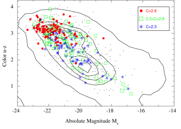
Figure 1: Distribution of the currently observed CALIFA galaxies in the $u-z$ vs. $M_{z}$ color-magnitude diagram. Different colors and symbols represent a classification into spheroid- and disk-dominated galaxies as well as intermediate cases, as suggested by the concentration index $C$ (see Sec. 2 for definition). For comparison, the contours delineate the number density distribution of galaxies in the SDSS-NYU catalogue (e.g. Blanton et al., 2005). The small dots indicate the remaining objects in the CALIFA mother sample, not observed so far.

The search for an explanation of the existence of radial gradients of abundances (and the G-dwarf metallicity distribution in MW) was the reason for the early development of chemical evolution models as well as the classical closed box model (CBM). The pure CBM, which relates the metallicity or abundance of a region to its fraction of gas, independently of the star formation or evolutionary history, was unable to explain the radial abundance gradient observed in our Galaxy and in other spirals. Therefore infall or outflows of gas in the MW were considered necessary to fit the data. In fact, as explained by Goetz & Koeppen (1992a), there are only 4 possible ways to create a radial abundance gradient: 1) A radial variation of the initial mass function (IMF); 2) A variation of the stellar yields with galactocentric radius; 3) A star formation rate (SFR) changing with the radius; 4) A gas infall rate variable with radius. The first possibility is not usually considered as probable, and the second one is already included in modern models, that adopt metallicity dependent stellar yields. Thus, from the seminal works of Lacey & Fall (1985a), Guesten & Mezger (1982) and Clayton (1987), most of numerical chemical evolution models (e.g. Diaz & Tosi, 1984; Matteucci & Francois, 1989a; Ferrini et al., 1992; Carigi, 1994; Prantzos & Aubert, 1995; Molla et al., 1996; Chiappini et al., 1997; Boissier & Prantzos, 1999b) explain the existence of the radial gradient of abundances by the combined effects of a star formation rate and an infall of gas, both varying with galactocentric radius of galaxies. In most recent times chemical evolution has been included in modern cosmological simulation codes, which already obtain spiral disks as observed, finding radial gradients of abundances which reproduce the data (Pilkington et al., 2012). It has been demonstrated Gibson et al. (2013), that the existence and evolution of these radial gradients is, as expected, very dependent on the star formation and infall prescriptions included in the simulations.

To characterize the properties of the ISM in the Local Universe and their relations with the evolution of galaxies, we applied the previously described procedure to the IFS data provided by the CALIFA survey (Sánchez et al., 2012a). CALIFA is an ongoing exploration of the spatially resolved spectroscopic properties of galaxies in the Local Universe ($z<$0.03) using wide-field IFS to cover the full optical extent (up to $\sim$3–4 r_e) of $\sim$600 galaxies of any morphological type, distributed across the entire color-magnitude diagram (Walcher et al., in prep.), and sampling the wavelength range 3650-7500 Å. So far, the survey has completed $\sim$1/2 of its observations, with 306 galaxies observed (May 2013), and the first data release, comprising 100 galaxies, was delivered in November 2012 Husemann et al. (2013).

In Sanchez et al. (2013) we presented the first results based on the catalog of H ii  regions extracted from these galaxies. We studied the dependence of the $\mathcal{M}$-Z relation with the star-formation rate, finding no secondary relation different from the one induced by the well known relation between the star formation and the mass. We confirm the local $\Sigma$-Z relation unveiled by Rosales-Ortega et al. (2011), with a larger statistical sample of H ii regions.

In the current study we will use the updated CALIFA catalog of H ii regions to study the radial oxygen abundance gradient up to 3-4 disk effective radii, well beyond the proposed break/flattening. The layout of this article is as follows: in Sec. 2 we summarize the main properties of the sample and data used in this study; in Sec. 3 we describe the analysis required to detect the individual clumpy ionized regions and aggregations, and to extract their spectroscopic properties, in particular the emission line ratios required to determine the abundance; the criteria to select the H ii region are explained in 3.3; the derivation of the abundance gradient for each galaxy is described in Sec. 4.1; in Sec. 4.2 we explore the dependence of the slope of these gradients with different morphological and structural properties of the galaxies; in Sec. 5.1 we describe the properties of the common gradient of the oxygen abundance for all disk galaxies up to $\sim$2 $r_{e}$, and the presence of a flattening beyond this radius; the drop of the abundance for some particular galaxies is shown in Sec. 5.3. Finally, the main conclusions of this study are discussed in Sec. 6.

2 Sample of galaxies and dataset

The galaxies were selected from the CALIFA observed sample. Since CALIFA is an ongoing survey, whose observations are scheduled on a monthly basis (i.e., dark nights), the list of objects increases regularly. The current results are based on the 306 galaxies observed before May 2013, i.e., half of the foreseen 600 galaxies to be observed at the end of the survey. Figure 1 shows the distribution of the current sample along the color-magnitude diagram, indicating with different symbols galaxies of different concentration index $C$ (defined to be the ratio $C=R_{90}/R_{50}$, where $R_{90}$ and $R_{50}$ are the radii enclosing 90% and 50% of the Petrosian r-band luminosity of the galaxy; i.e., a proxy of the morphological type). The current sample covers all the color-magnitude diagram, up to $M_{z}<-17$ mag, with at least three targets per bin of $\sim$1 magnitude and color ($\sim$10 galaxies on average) including galaxies of any morphological type. The CALIFA mother sample becomes incomplete below $M_{r}>-19$ mag, which corresponds to a stellar mass of $\sim$10^9.5 M_⊙ for a Chabrier IMF. Therefore, it does not sample properly the low-mass and/or dwarf galaxies. Above this luminosity, the sample is representative of the total population at the selected redshift range (0.005$<z<$0.03), and in principle it should be representative of galaxies at the Local Universe.

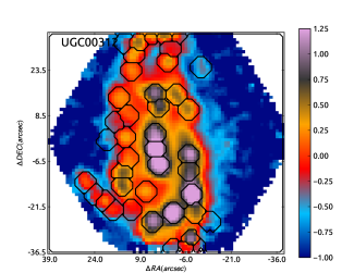
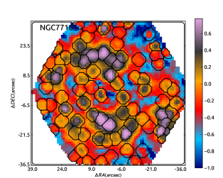
Figure 2: IFS-based H$\alpha$ maps, in units of ($\log_{10}$) 10^-16 erg s^-1 cm^-2 arcsec^-2, derived for two representative galaxies of the sample, together with the detected H ii regions shown as black segmented contours.

The details of the survey, sample, observational strategy, and reduction are explained in Sánchez et al. (2012a). All galaxies were observed using PMAS (Roth et al., 2005) in the PPAK configuration (Kelz et al., 2006), covering a hexagonal field-of-view (FoV) of 74$\arcsec$$\times$64$\arcsec$, sufficient to map the full optical extent of the galaxies up to 2-3 disk effective radii. This is possible because of the diameter selection of the sample (Walcher et al., in prep.). The observing strategy guarantees a complete coverage of the FoV, with a final spatial resolution of FWHM$\sim$3$\arcsec$, corresponding to $\sim$1 kpc at the average redshift of the survey. The sampled wavelength range and spectroscopic resolution (3745-7500Å, $\lambda/\Delta\lambda\sim$850, for the low-resolution setup) are more than sufficient to explore the most prominent ionized gas emission lines, from [OII]$\lambda$3727 to [SII]$\lambda$6731, on one hand, and to deblend and subtract the underlying stellar population, on the other hand (e.g. Sánchez et al., 2012a; Kehrig et al., 2012; Cid Fernandes et al., 2013). The dataset was reduced using version 1.3c of the CALIFA pipeline, whose modifications with respect to the one presented in Sánchez et al. (2012a) are described in detail in Husemann et al. (2013). In summary, the data fulfil the predicted quality-control requirements, with a spectrophotometric accuracy better than 15% everywhere within the wavelength range, both absolute and relative, and a depth that allows us to detect emission lines in individual H ii  regions as weak as $\sim$10^-17erg s^-1 cm^-2, with a signal-to-noise ratio of S/N$\sim$3-5. For the emission lines considered in the current study the S/N is well above this limit, and the measurement errors are neglectable in most of the cases. In any case, they have been propagated and included in the final error budget.

The final product of the data-reduction is a regular-grid datacube, with $x$ and $y$ coordinates indicating the right-ascension and declination of the target and $z$ being a common step in wavelength. The CALIFA pipeline also provides the propagated error cube, a proper mask cube of bad pixels, and a prescription of how to handle the errors when performing spatial binning (due to covariance between adjacent pixels after image reconstruction). These datacubes, together with the ancillary data described in Walcher et al. (in preparation), are the basic starting point of our analysis.

The observing strategy of the CALIFA survey guarantees that the main properties of the observed sample are compatible with those of the mother sample, in terms of luminosities, sizes, morphologies and colors (Sánchez et al., 2012a; Husemann et al., 2013). Particular care is taken to not introduce any potential observational bias, as the targets are selected in a pseudo-random way based only on the visibility from the observatory on a monthly basis (i.e., dark-time). In Walcher et al. (in prep.), we will describe the main properties of the CALIFA mother sample. In summary we can claim that with our selection criteria our sample does not under-represent any kind of galaxies in the Local Universe in any observable within our 95% completeness range ($-$23$<$M_r,SDSS$<-$19 mag). Obviously our results are restricted to this particular range, and therefore cannot be applied to either dwarf or giant elliptical galaxies, which are under-represented or absent in our sample.

3 Analysis

The main goal of this study is to characterize the abundance gradient in galaxies, and determine if there are common patterns and/or differences depending on their individual properties. Ionized gas abundances have been well calibrated on the basis of strong-line indicators for ionized regions associated with star formation processes, i.e., the classical H ii regions. In this section we describe how we have selected those regions, extract and analyze their individual spectra, derive the corresponding oxygen abundance and, finally, analyze their radial gradient.

3.1 Detection of ionized regions

The segregation of H ii regions and the extraction of the corresponding spectra is performed using a semi-automatic procedure named HIIexplorer. The procedure is based on some basic assumptions: (a) H ii regions are peaky/isolated structures with a strong ionized gas emission, that is significantly above the stellar continuum emission and the average ionized gas emission across the galaxy. This is particularly true for H$\alpha$; (b) H ii regions have a typical physical size of about a hundred or a few hundred parsecs (e.g. González Delgado & Perez, 1997; Lopez et al., 2011; Oey et al., 2003), which corresponds to a typical projected size of a few arcsec at the distance of the galaxies.

These basic assumptions are based on the fact that most of the H$\alpha$ luminosity observed in spiral and irregular galaxies is a direct tracer of the ionization of the inter-stellar medium (ISM) by the ultraviolet (UV) radiation produced by young high-mass OB stars. Since only high-mass, short-lived, stars contribute significantly to the integrated ionizing flux, this luminosity is a direct tracer of the current star formation rate (SFR), independent of the previous star formation history. Therefore, clumpy structures detected in the H$\alpha$ intensity maps are most probably associated with classical H ii regions (i.e., those regions for which the oxygen abundances have been calibrated).

The details of HIIexplorer are given in Sánchez et al. (2012b) and Rosales-Ortega et al. (2012). We present here the basic steps included in the overall process: (i) First we create a narrow-band image of 120$\AA$ width, centered on the wavelength of H$\alpha$ shifted at the redshift of each target. The image was created by co-adding the flux within the described spectral window for each spaxel of the velocity-field corrected datacube. Then, the image is properly corrected for the underlying adjacent continuum. (ii) This image is used as an input for the automatic H ii region detection algorithm included in HIIexplorer. In this particular case, the algorithm detects iteratively the peak intensity emission above a threshold of 4$\times$10^-17 erg s^-1 cm^-2 arcsec^-1, and then assigns all the adjacent pixels up to a distance of 3.5$\arcsec$, with a flux within a 10% of the peak intensity ($I_{pixel}>0.9\times I_{peak}$), and above a limiting flux intensity of 1$\times$10^-17 erg s^-1 cm^-2 arcsec^-1 into the corresponding area. Once the first region is detected and segregated, the corresponding area is masked from the input image, and the procedure is repeated until there are no additional regions to be selected. The remaining pixels are assigned to a residual region which is assumed to be dominated by diffuse emission. The result is a segmentation map that segregates each detected cumpy ionized structure. Finally, (iii) the integrated spectra corresponding to each segmented region is extracted from the original datacube, and the corresponding position table of the detected H ii is provided. If the object was has been observed in both the low-resolution and high-resolution modes (Sánchez et al., 2012a), both corresponding spectra were extracted.

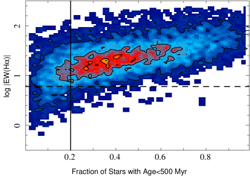
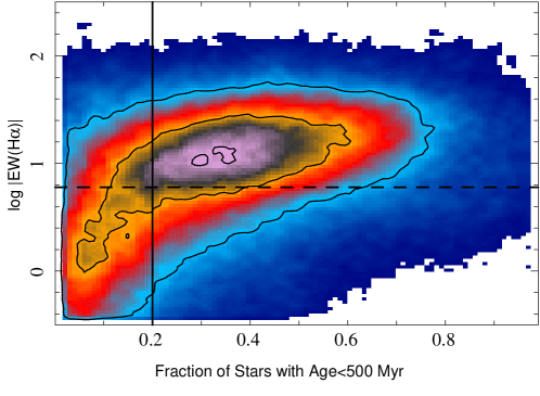
Figure 3: Left-panel: Absolute value of the equivalent width of H$\alpha$, on a logarithmic scale, plotted against the fraction of young stars in the underlying stellar population (according to the SSP modelling by FIT3D) for the clumpy ionized regions selected with HIIexplorer. Right-panel: Similar distribution of the emission equivalent width of H$\alpha$, on a logarithmic scale, along the luminosity fraction of young stars in the underlying stellar population for the $\sim$500,000 individual spaxels with H$\alpha$ emission detected in the 306 analysed datacubes. In both panels, the dashed horizontal line shows the demarcation limit of the EW of H$\alpha$ proposed by Cid Fernandes et al. (2010) to distinguish between strong (star formation and/or AGNs) and weak (e.g., post-AGBs) ionization sources. The vertical solid line shows the currently adopted selection criteria for the H ii regions.

Figure 2 illustrates the process, showing the H$\alpha$ intensity maps and the corresponding segmentations for two objects: (1) UGC00312, an intermediate-to-high inclined ($\sim$70 degrees), not very massive ($\sim$0.7$\times$10¹⁰ M_⊙) and almost bulge-less spiral galaxy, and (2) NGC7716, a low inclination ($<$40 degrees), massive ($\sim$2$\times$10¹⁰ M$\odot$) spiral, with a clear bulge. These two galaxies illustrate why for highly inclined galaxies we cover up to 4-5 disk effective radii (mostly along the semi-minor axis), while for mostly face-on ones we cover just half of this size, although both galaxies were diameter selected (Sánchez et al., 2012a). The galaxies analyzed in Sánchez et al. (2012b), are more similar to the second type, and therefore the region beyond $\sim$2 effective radii was mostly unexplored.

A total of 7016 individual clumpy ionized regions are detected in a total of 227 galaxies from the sample, i.e., $\sim$30 H ii regions per galaxy. This does not mean that on averarage there is no ionized gas in the remaining 79 galaxies. Recent results indicate that it is possible to detect low-intensity (and in most cases low-ionization) gas in all the analyzed CALIFA galaxies (Kehrig et al., 2012; Papaderos et al., 2013; Singh et al., 2013). As discussed in Papaderos et al. (2013), and in line with a substantial body of previous works (Sarzi et al., 2010; Annibali et al., 2010; Yan & Blanton, 2012; Kehrig et al., 2012, among others), various lines of evidence suggest that photoionization by post-AGB stars appears to be the main driver of extended nebular emission in these systems, with non-thermal sources being potentially important only in their nuclei. The observational evidence behind this conclusion is that the nebular emission is not confined only to the nuclear regions but is extended out to r $\sim$2–4 r₅₀, i.e. it is co-spatial with the post-AGB stellar background. In most of these cases EW(H$\alpha$) typically is $\sim$ 1 Å. In other cases the ionized gas does not present clear clumpy structures, required to associate them with starforming/H ii regions. This is the case of the shock ionized regions detected in the MICE galaxies (Wild et al., submitted). Since most of this ionization is not associated with young massive stars, and therefore the associated abundances are not well calibrated, it is not relevant for the present analysis.

3.2 Measurement of the emission lines

To extract the nebular physical information of each individual H ii region, the underlying stellar continuum must be decoupled from the emission lines for each of the analyzed spectra. Several different tools have been developed to model the underlying stellar population, effectively decoupling it from the emission lines (e.g., Cappellari & Emsellem, 2004; Cid Fernandes et al., 2005; Ocvirk et al., 2006; Sarzi et al., 2006; Sánchez et al., 2006b; Koleva et al., 2009; MacArthur et al., 2009; Walcher et al., 2011). Most of these tools are based on the same principles, i.e., they assume that the stellar emission is the result of the combination of different (or a single) simple stellar populations (SSP), and/or the result of a particular star-formation history, whose corresponding emission-line spectrum is redshifted due to a certain systemic velocity, broadened and smoothed by the effect of a certain velocity dispersion and attenuated by a certain dust content.

We performed a simple modeling of the continuum emission using FIT3D, a fitting package described in Sánchez et al. (2006b) and Sánchez et al. (2011). A simple SSP template grid with 12 individual populations was adopted. It comprises four stellar ages (0.09, 0.45, 1.00 and 17.78 Gyr), two young and two old ones, and three metallicities (0.0004, 0.019 and 0.03), sub-solar, solar and super-solar. The models were extracted from the SSP template library provided by the MILES project (Vazdekis et al., 2010; Falcón-Barroso et al., 2011). The use of different stellar ages and metallicities or a larger set of templates does not affect qualitatively the derived quantities that describe the stellar populations. Evenmore, it does not affect quantitatively the estimations of the properties of the emission lines.

The analysis of the underlying stellar population is not as detailed as the one presented by Cid Fernandes et al. (2013), and it is not useful to reconstruct the star formation history. However, since the spatial binning required to define these regions is based on the H$\alpha$ intensity, in many cases the extracted spectra of the underlying stellar continuum do not reach the required signal-to-noise to perform a more detailed analysis. We prefer to restrict our stellar fitting to a reduced template library with few stellar populations, and derive simple conclusions, such as the fraction of young or old stars. Therefore, we will not pay too much attention to the actual decomposition in different populations.

Throughout, we adopted the Cardelli et al. (1989) law for the stellar dust attenuation with an specific attenuation of $R_{\rm V}=3.1$, assuming a simple screen distribution. The use of different laws, like the one proposed by Calzetti (2001), does not produce significant differences in the modelling of the underlying stellar population in the wavelength range considered. A different amount of extinction, parametrized by the extinction in the V-band ($A_{V}$), was considered for each stellar population. We consider that this is more realistic than to assume the same attenuation for all the stellar populations, since the distribution of the dust grains is not homogeneous, and it affects the old and young stellar populations in a different way.

Individual emission line fluxes were measured using FIT3D in the stellar-population subtracted spectra performing a multi-component fitting using a single Gaussian function. When more than one emission line was fitted simultaneously (e.g., for doublets and triplets, like the [N ii] lines), the systemic velocity and velocity dispersion were forced to be equal, in order to decrease the number of free parameters and increase the accuracy of the deblending process. The ratio between the two [N ii] lines included in the spectral range were fixed to the theoretical value (Osterbrock & Ferland, 2006). By adopting this procedure it is possible to accurately deblend the different emission lines. A similar procedure was applied to the rest of the lines which were fitted simultaneously (e.g. H$\beta$ and [O iii]). The measured lines include all lines employed in the determination of metallicity using strong-line methods, i.e H$\alpha$, H$\beta$, [O ii] $\lambda$3727, [O iii] $\lambda$4959, [O iii] $\lambda$5007, [N ii] $\lambda$6548, [N ii] $\lambda$6583, [S ii] $\lambda$6717 and [S ii] $\lambda$6731. Additionally, for those H ii regions with high signal-to-noise we were able to detect and measure intrinsically fainter lines such as [Ne III] $\lambda$3869, H$\epsilon$ $\lambda$3970, H$\delta$ $\lambda$4101, H$\gamma$ $\lambda$4340, He I $\lambda$5876, [O I] $\lambda$6300, and He I $\lambda$6678, although they have not been considered for the present study. FIT3D provides the intensity, equivalent width, systemic velocity and velocity dispersion for each emission line. The statistical uncertainties in the measurements were calculated by propagating the error associated with the multi-component fitting and considering the signal-to-noise of the spectral region. Note that by subtracting a stellar continuum model derived with a set of SSP templates, we are already correcting for the effect of underlying stellar absorption, which is particularly important in Balmer lines (such as H$\beta$). We performed a series of sanity tests based on the H$\alpha$/H$\beta$ ratio to ensure that no overcorrection was done on the absorption stellar features.

Note that FIT3D fits the underlying stellar population and the emission lines together. Therefore, in addition to the parameters derived for the emission lines, the fitting algorithm provides us with a set of parameters describing the physical components of the stellar populations. In particular it provides the fraction of light that contributes to the continuum at 5000Å corresponding to an old ($>$500 Myr, $f_{o}$) or young ($<$500 Myr, $f_{y}$) stellar population (which we consider a reliable parameter for our current stellar analysis).

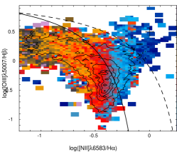
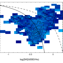
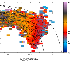
Figure 4: Left panel: [O iii] $\lambda$5007/H$\beta$ vs. [N ii] $\lambda$6583/H$\alpha$ diagnostic diagram for the $\sim$7000 ionized regions described in the text. The contours show the density distribution of these regions with the diagram plane, with the outermost contour enclosing 95% of the regions, and each consecutive one enclosing 20% less regions. The color indicate the fraction of young stellar population in the underlying continuum. Central panel: Same diagnostic diagram, restricted to those ionized regions with less than a 20% of young stellar population ($\sim$1800 regions). Right panel: Same diagnostic diagram, restricted to those ionized regions with more than a 20% of young stellar population ($\sim$5800 regions). In all the panels, the solid- and dashed-line represent, respectively, the Kauffmann et al. (2003) and Kewley et al. (2001) demarcation curves. They are usually invoked to distinguish between classical star-forming objects (below the solid-line), and AGN powered sources (above the dashed-line). Regions between both lines are considered intermediate ones.

3.3 Selection of the H ii regions

Classical H ii regions are gas clouds ionized by short-lived hot OB stars, associated with on-going star formation. They are frequently selected on the basis of demarcation lines defined in the so-called diagnostic diagrams (e.g. Baldwin et al., 1981; Veilleux & Osterbrock, 1987), which compare different line ratios, such as [OIII]/H$\beta$ vs [NII]/H$\alpha$, [OIII]/H$\beta$ vs [OII]/H$\alpha$, [NII]/H$\alpha$ vs. [SII]/H$\alpha$ and/or [NII]/H$\alpha$ vs. [SII]/$H\alpha$. In most cases these ratios discriminate well between strong ionization sources, like classical H ii regions and powerful AGNs (e.g. Baldwin et al., 1981). However, they are less accurate in distinguishing between low-ionization sources, like weak AGNs, shocks and/or post-AGBs stars (e.g. Cid Fernandes et al., 2011; Kehrig et al., 2012). Alternative methods, based on a combination of the classical line ratios with additional information regarding the underlying stellar population have been proposed. For example, Cid Fernandes et al. (2011) proposed the use of the EW(H$\alpha$), to distinguish between retired (non starforming) galaxies, weak AGNs and star-forming galaxies.

The most common diagnostic diagram in the literature for the optical regime is the one which makes use of easily-observable strong lines that are less affected by dust attenuation, i.e., [O iii]/H$\beta$ vs. [N ii]/H$\alpha$ (Baldwin et al., 1981). We will refer hereafter to this diagnostic diagram as the BPT diagram. Different demarcation lines have been proposed for this diagram. The most popular ones are the Kauffmann et al. (2003) and Kewley et al. (2001) curves. They are usually invoked to distinguish between star-forming regions (below the Kauffmann et al., 2003, curve), and AGNs (above the Kewley et al., 2001, curve) . The location between both curves is normally assigned to a mixture of different sources of ionization. Additional demarcation lines have been proposed for the region above the Kewley et al. (2001) curve to segregate between Seyfert and LINERs (e.g., Kewley et al., 2006).

Despite of the benefits of this clean segregation for classification purposes, it may introduce biases when applied in order to select H ii regions. The Kewley et al. (2001) curve was derived on the basis of photoionization models. It corresponds to the maximum envelope in the considered plane for ionization produced by hot stars. Therefore, to the extent that these models are realistic enough, any combination of line ratios below this curve can be produced entirely by OB star photoionization. Finally, it defines all the area above it as un-reachable by ionization associated with star-formation. The Kauffmann et al. (2003) curve has a completely different origin. It is an empirical envelope defined to segregate between star-forming galaxies and the so-called AGN branch in the BPT diagram based on the analysis of the emission lines for the SDSS galaxies. It describes well the envelope of classical H ii regions found in the disks of spiral galaxies. However, it is known that certain H ii regions can be found above this demarcation line, as we will show below.

Kennicutt et al. (1989) first recognized that H ii regions in the center of galaxies distinguish themselves spectroscopically from those in the disk by their stronger low-ionization forbidden emission. The nature of this difference was not clear. It may be due to contamination by an extra source of ionization, like diffuse emission or the presence of an AGN. However, other stellar processes, such as nitrogen enhancement due to a natural aging process of H ii regions and the surrounding ISM can produce the same effect. These early results were confirmed by Ho et al. (1997), who demonstrated that inner star-forming regions may populate the right branch of the BPT diagram, at a location above the demarcation line defined later by Kauffmann et al. (2003). However, we have found that these H ii regions are not restricted to the central regions, and can be found at any galactocentric distance, even at more than 2 $r_{e}$ (Sec. 5.1), which excludes the contamination by a central source of ionization. The nature of these H ii regions will be addressed in detail elsewhere. For the purpose of the current study it is important to define a selection criterion that does not exclude them.

Therefore, selecting H ii regions based on the Kauffmann et al. (2003) curve may bias our sample towards classical disk regions, excluding an interesting population of these objects. On the other hand it does not guarantee the exclusion of other sources of non-stellar ionization that can populate this area, like shocks (e.g. Allen et al., 2008; Levesque et al., 2010), post-AGB stars (e.g. Kehrig et al., 2012) and dusty AGNs (e.g. Groves et al., 2004). Following Cid Fernandes et al. (2010) and Cid Fernandes et al. (2011), we consider that an alternative method to distinguish between different sources of ionization is to compare the properties of the ionized gas with that of the underlying stellar population.

We adopted a different selection criterion, using the fraction of young stars ($f_{y}$) provided by the multi-SSP analysis of the underlying stellar population, as a proxy for the star-formation activity. For star-forming regions this parameter provides similar information to the EW(H$\alpha$). Figure 3, left-panel, shows the distribution of EW(H$\alpha$) against the fraction of young stars for the $\sim$7000 clumpy ionized regions selected by HIIexplorer. For those regions with EW(H$\alpha$)$>$6 Å, and/or with a fraction of young stars larger than 20%, both parameters present a strong log-linear correlation ($r_{corr}=$0.95). Fig 3, right-panel, shows the same distribution for the $\sim$500,000 spaxels with detected H$\alpha$ emission. This distribution presents the same trend described before, but with an evident tail towards lower EW(H$\alpha$) values and a lower fraction of young stars.

The threshold imposed by HIIexplorer in the surface brightness of H$\alpha$ and the requirement that the ionization is clumpy efficiently removes most of the ionization corresponding to weak-emission lines described. This is mostly diffuse emission, that peaks in the described diagram at EW(H$\alpha$)$\sim$1-2 Å and $f_{y}\sim$5-10%. For early-type galaxies, this weak EW(H$\alpha$) is mostly by post-AGB stars (e.g. Kehrig et al., 2012; Papaderos et al., 2013), and therefore no correlation is expected between its intensity and the fraction of young stars (as explained before in Sec. 3.1). On the other hand, high EW(H$\alpha$) could be produced by other mechanisms, like AGNs and shocks, that are not required to be correlated in principle with the properties of the underlying stellar population. A cut in the EW(H$\alpha$) cannot remove those regions. Therefore, we consider that the fraction of young stars provides, in connection with the aforementioned spectroscopic classification criteria, a robust and physically motivated means or the extraction of genuine H ii regions.

Figure 4, left-panel, shows the distribution of the ionized regions across the BPT diagram, with contours indicating the density of regions at each location. The outermost of those contours encloses 95% of the detected regions, with each consecutive one encircling fewer regions. This contour is located below the Kewley et al. (2001) demarcation curve, which indicates that the ionization of our selected clumpy regions is already dominated by star formation. In fact, only $\sim$2% of all regions are located above the Kewley et al. (2001) line, and $\sim$80% are below the Kauffmann et al. (2003) line (i.e., where classical disk H ii regions are located). If we had adopted this latter demarcation curve as our selection criteria we would have missed a significant number of regions.

The color-code in Fig 4 indicates the average fraction of young stars at each location (i.e., the $x$-axis in Fig. 3), ranging from nearly 100% for the regions at the top-left area of the diagram, to nearly 0% for regions at the top-right location. There is a clear gradient/correlation between the fraction of young stars and the [N ii]/H$\alpha$ ratio, reflecting the known downsizing-like variation of the specific SFR along the SF branch of the BPT diagram (Asari et al., 2007).

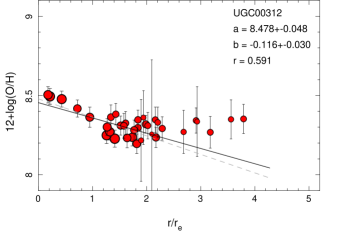
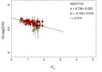
Figure 5: Radial distribution of the oxygen abundance derived for the individual H ii regions with abundance errors below 0.15 dex, as a function of the deprojected galactocentric distance (i.e., corrected for inclination), normalized to the disk effective radius, for the galaxies presented in Fig. 2. The size of the symbols is proportional to the H$\alpha$ intensity. The red circles represent those H ii regions below the Kauffmann et al. (2003) line, and the orange squares represent those ones above this curve and below the Kewley et al. (2001) demarcation lines, i.e., the regions at the so called intermediate zone in the BPT diagram. The solid and dashed lines show the best linear regression and error-weighted linear fit derived for those values between 0.3 and 2.1 $r_{e}$. The results from the second fit are shown in the figure, including the zero-point (a), slope (b), and correlation coefficient (r).

Based on these results, we classified as H ii regions those clumpy ionized regions for which young stars ($<$500 yr) contribute at least a 20% to the flux in the $V$-band. This particular fraction is the lowest for which the correlation coefficient between $f_{y}$ and the EW(H$\alpha$) is still higher than $r_{corr}>$0.95, and for which the fraction of excluded regions is not higher than the one that would be excluded by adopting the more common Kauffmann et al. (2003) curve. Fig. 4, central panel, shows the same distribution as the one shown in the left panel, but restricted to the 1787 regions for which the fraction of young stars is lower than 20%. The fraction of regions above the Kewley et al. (2001) curve is significantly larger ($\sim$7%), with more than a 40% above the Kauffmann et al. (2003) one. Although there are still 1043 regions below this latter curve, it comprises just $\sim$15% of the original sample. This can be considered our incompleteness fraction. Although we cannot exclude that some fraction of these regions are ionized by star-formation, we cannot guarantee it.

Fig. 4, right panel shows the same distribution, but for the 5229 regions with a fraction of young stars larger than 20%, i.e., our final sample of H ii regions. Of them, only 23 are above the Kewley et al. (2001) curve ($\sim$99.5% are below it). On the other hand, there are 713 regions in the so-called intermediate region, with a significant fraction of young stars ($\sim$40% on average). These regions would have been excluded if we had adopted the Kauffmann et al. (2003) curve as our selection criteria, and we would have lost a certain number of H ii regions at any galactocentric distance. We consider that the adopted combined selection criteria are more physically driven and conservative, since they select only those regions that are associated with an underlying stellar population indicative of the presence of young stars.

4 Results

4.1 Oxygen abundance gradients

In order to derive the oxygen abundance for each of the selected $\sim$5000 H ii regions, we adopted the empirical calibrator based on the O3N2 ratio (Alloin et al., 1979; Pettini & Pagel, 2004; Stasińska et al., 2006).

$${\rm O3N2} = {\rm log_{\rm 10}}\left[\frac{I([@series{\mathbf{O\,\mathsc{iii}}}]\leavevmode\nobreak\ \lambda 5007)/I({\rm H}\beta)}{I([@series{\mathbf{N\,\mathsc{ii}}}]\leavevmode\nobreak\ \lambda 6584)/I({\rm H}\alpha)}\right]$$ (1)

This ratio is basically not affected by the effects of dust attenuation, uses emission lines covered by our wavelength range for all the galaxies in the sample, and it has a monotonic single-valued behavior in its range of applicability. We adopted the functional form and calibration by Pettini & Pagel (2004), although its correspondence with temperature-anchored abundances at the high-metallicity range is still under debate (Marino et al., 2013). In that article we demonstrate that the indicator is valid for a range of line ratios between $-$1.1$<$O3N2$<$1.7, which corresponds to oxygen abundances above 12+log(O/H)$>$8 dex. In our sample of H ii regions we do not reach the low metallicity limit for which the calibration is still useful, most probably because we do not include low-mass/dwarf galaxies in the considered sample of galaxies. In this regime the derived abundances have an accuracy of $\pm$0.08 dex, an uncertainty that has been included in the error budget. The typical error derived from the pure propagation of the errors in the measured emission lines is about 0.05 dex, although in a few cases is can be larger.

It is beyond the scope of the current study to make a detailed comparison of the oxygen abundances derived using the different proposed methods, such as was presented by Kewley & Ellison (2008) or López-Sánchez et al. (2012). However, we want to state clearly that all our qualitative results and most of the quantitive ones are mostly independent of the adopted oxygen abundance calibrator, i.e. despite the absolute scale among the different indicators and the differences introduced by them in the galaxy slopes, the abundance gradients show statistically the same relationships with respect to global galaxy properties, as explained below.

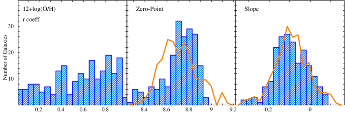
Figure 6: Left panel: Distribution of correlation coefficients of the oxygen abundance along the radial distance, for the 193 galaxies described in the text. Central panel: Distribution of zero-points for the corresponding linear regression galaxy by galaxy. Right panel: Distribution of slopes of the same regressions. The orange solid line represents, for each of the last two histograms, the expected histogram in case of a Gaussian distribution of the data, assuming the mean and standard-deviation of the distribution of each analyzed parameter, and sampled with the same bins.

We derive for each galaxy the galactocentric radial distribution of the oxygen abundance, based on the abundances measured for each individual H ii region. In Appendix A we describe the surface-brightness and morphological analysis performed for each galaxy to derive the mean position angle, ellipticity, and effective radius of the disk. Using this information we deprojected the position of each H ii region for each galaxy, assuming an intrinsic ellipticity for galaxies of $q=$0.13 (Giovanelli et al., 1995, 1997), and an inclination given by:

$${\rm cos^{2}i=\frac{1-q^{2}-\epsilon^{2}}{1-q^{2}}}$$ (2)

where $i$ is the inclination of the galaxy, and $\epsilon$ is the median ellipticity provided by the morphological analysis, defined for each galactocentric distance as:

$${\rm\epsilon^{2}=1-\left(\frac{a}{b}\right)^{2}}$$ (3)

where $a$ and $b$ are the semi-major and semi-minor axes. For galaxies with an inclination below 35^∘ we prefer not to correct for the inclination effects due to the uncertainties in the derived correction, and the very small effect on the spatial distribution of H ii regions. We derive the galactocentric distance for each region, which is later normalized to the disk effective radius ($r_{e}$). This disk effective radius was derived from the scale-length of the disk of each galaxy, extracted from the analysis of the surface brightness profile in the $g$-band as detailed in the Appendix A. For disk dominated galaxies this effective radius is similar to the classical effective radius, that can be derived by a pure growth-curve for the full light distribution of the galaxy. However, for galaxies with a clear bulge it represents the characteristic scale of only the disk part. The center of the galaxy was taken from the WCS of the cube headers, and it was derived by a barycenter estimation described in Husemann et al. (2013).

Finally, for each galaxy we derive the oxygen abundance gradient. Figure 5 shows two examples of these abundance gradients for the same galaxies shown in Figure 2 (i.e. UGC 00312, left-panel, with high inclination and NGC 7716, right-panel, with low inclination). As we indicated before, the CALIFA FoV covers on average $\sim$2.5 $r_{e}$ of the observed galaxies. However, due to the inclination for spiral galaxies this FoV has a wide range between $\sim$2 $r_{e}$ for the face-on galaxies and up to $\sim$5 $r_{e}$ for the edge-on ones (although the particular range depends also on the intrinsic characteristics of the galaxies).

Following this analysis we perform a linear regression, without considering the errors of the individual abundances, and an error-weighted linear fit to the radial distribution of abundances galaxy-by-galaxy, restricted to the same spatial range. From the original 227 galaxies with detected ionized regions, we restricted the analysis to those with at least four H ii regions within the considered spatial range (0.3$<r/r_{e}<$2.1). Although Zaritsky et al. (1994) found empirically that at least five H ii regions are required to define the slope, we found that this depends also on the individual errors, the range of abundances and galactocentric distances sampled, and the actual signal-to-noise. Based on a Monte-Carlo simulation we found that for less than four H ii regions in a galaxy the derived slope is not reliable. This final sample comprises 193 galaxies, and a total of 4610 H ii regions. 94 galaxies show at least one region beyond 2.2 disk effective radius, with a total of 484 regions (i.e, $\sim$5 regions per galaxy in this outer region, on average).

The result of this analysis is illustrated is Fig. 6, where we show the distribution of the correlation coefficients, zero-points, and slopes for each individual galaxy. For most of the galaxies there is a clear correlation between the oxygen abundance and the radial distance. The correlation coefficient (shown on the left-panel of Fig. 6) is larger than $r_{corr}>$0.4 for $\sim$72% of the galaxies. This $r_{corr}$ corresponds to a probability of good fit of $\sim$98.5% for the typical number of H ii regions in our galaxies. Most of the galaxies for which the correlation coefficient is lower than this value are galaxies with low number of detected H ii regions. The distribution of zero-points (mid-panel) has a mean value at 12+log(O/H)$\sim$8.73 dex with a standard deviation of $\sigma\sim$0.16 dex, with a range of values reflecting the mass-range covered by the sample, due to the well-known $\mathcal{M}$-Z relation (e.g. Tremonti et al., 2004; Sanchez et al., 2013). Finally, the distribution of slopes (right-panel of Fig. 6) has a clear peak and it is remarkably symmetric. The probability of being compatible with a Gaussian distribution is 98%, based on a Lilliefors-test (Lilliefors, 1967) (compared with 77% derived for the distribution of zero-points). Therefore, the slopes of the abundance gradients have a well-defined characteristic value of $\alpha_{O/H}=-$0.10 dex/$r_{e}$ with a standard deviation of $\sigma=$0.09 dex/$r_{e}$, totally compatible with the value reported in Sánchez et al. (2012b), for a more reduced sample. This slope corresponds to an $\alpha_{O/H}=-$0.06 dex/$r_{d}$, when normalized to the disk scale-length ($r_{d}$), instead of the disk effective radius ($r_{e}$). If instead of this normalization scale, we adopt a more classical one, like $r_{25}$ (the radius at which the surface-brightness reaches 25 mag/arcsec² in the B-band) we obtain a similar result, although for a sharper slope of $\alpha_{O/H}=-$0.16 dex/$r_{25}$, and a dispersion of $\sigma=$0.12 dex/$r_{25}$. Finally, if the physical scale (i.e., kpc) at the distance of the galaxy is used instead of any of the previous normalizations, then we find a shallower average slope of $\alpha_{O/H}=-$0.03 dex/kpc with a standard deviation of $\sigma=$0.03 dex/kpc. Even more important, for this final case the distribution is not asymmetric, presenting a clear tail towards large slopes, up to $-$0.15 dex/kpc.

4.2 Abundance gradient by galaxy types

In this section we analyze the possible dependence of the slope of the gradients on the properties of the galaxies. But before addressing this issue we point out some possible limitations and biases affecting the analysis performed. Figure 7, left panel, shows the distribution of the number of detected H ii regions as a function of the inclination of the galaxy. It is clear that although the number of H ii regions is not the only parameter that affects this error, for galaxies with less than $\sim$10 regions the error is considerably larger. On the other hand the number of detected regions decreases with increasing inclination. For highly inclined galaxies ($i>70^{\circ}$), there are very few galaxies with more than 15 H ii regions. This is a clear selection effect, since highly inclined galaxies have less accessible portion of the disk, and therefore the number of detected regions is reduced. We have taken into account this bias in the following analysis.

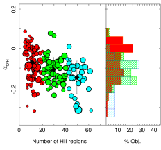
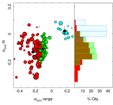
Figure 7: Left panel: Number of detected H ii regions as a function of the inclination of the galaxy. The colors of the symbols and the corresponding histogram indicate the inclination of the galaxies: (i) Less than 45^∘ (red), (ii) between 45^∘ and 65^∘ (green) and (iii) larger than 65^∘ (blue). Central panel: Slope of the gradients of the oxygen abundance derived for each galaxy along the number of detected H ii regions. The colors of the symbols and the corresponding histogram indicate the number of detected H ii regions in each galaxy: (i), Less than 20 H ii regions (red), (ii) between 20 and 40 H ii regions (green) and (iii) more than 40 H ii regions (blue). Right panel: Slope of the gradients of the oxygen abundance derived for each galaxy based on the linear regression of the radial distribution along the slope derived by comparing the range of abundances with the corresponding range of radial distances. The colors of the symbols and the corresponding histogram indicate this latter parameter, showing (i) slopes lower than than $-$0.25 dex/$r_{e}$ (red), (ii) between $-$0.25 and 0.05 dex/$r_{e}$ (green) and (iii) larger than 0.05 dex/$r_{e}$ (blue). The size of the symbols are inversely proportional to the derived error in the slope of the abundance gradient, in both panels. The black-solid diamonds represent the mean values for the different selected subsamples, with the error bars indicating the standard deviation around this mean value.

Fig 7, central panel, shows the distribution of the slopes as a function of the number of detected H ii regions, including galaxies of any inclination. For galaxies with few detected regions there is a strong secondary peak in the distribution at $\alpha_{O/H}\sim$0 (i.e., a constant value). This secondary peak is more evident in the right panel, where we compare the slopes derived from the linear regression (i.e., those shown in the central panel and in Fig. 6), with a rough estimation of the slope derived by dividing the range of abundances within the considered galactocentric distances ($0.3-2.1$ $r_{e}$), by the differences of radial distances,

$${\rm\alpha_{range}=\frac{max[12+log(O/H)]-min[12+log(O/H)]}{r_{max\ O/H}-r_{min\ O/H}}}.$$ (4)

This parameter is more sensitive to the actual range of abundances measured for the H ii regions in each galaxy. Most of the galaxies are concentrated in a cloud around $(\alpha_{O/H},\alpha_{range})=(-0.1,-0.15)$ (with a wide dispersion in the second parameter). However, there is a second group of galaxies with nearly flat or even inverse gradients (indicated with a blue color), which are mostly galaxies with a low number of H ii regions and/or highly inclined galaxies. It is clear that for those galaxies our derived slope is less reliable. Thus, better determinations of the slope will result for (i) larger number of H ii regions, (ii) larger range of abundances, and (iii) larger covered range of galactocentric distances.

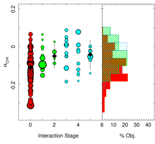
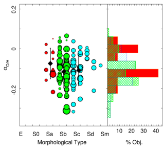
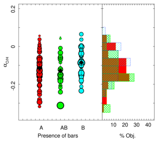
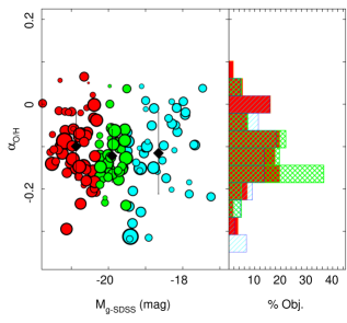
Figure 8: Top-left panel: Distribution of the slopes of the abundance gradients as a function of the interaction stage of the galaxies. The colors of the symbols and the corresponding histograms indicate three types of galaxies based on the interaction: (i) no signatures of interaction (red), (ii) galaxies with close companions and/or in an early interaction stage (green), and (iii) galaxies under clear coalescence or evolved mergers (blue). Top-right panel: Similar distribution of slopes as a function of the morphological classification of the galaxies. The colors of the symbols and the corresponding histograms indicate three types of galaxies based on their morphology: (i) Early spirals, SO-Sa (red), (ii) intermediate spirals, Sab-Sb (green) and (iii) Late spirals, Sc-Sm (blue). Bottom-left panel: Similar distribution of slopes as a function of the presence or absence of bars. The colors of the symbols and the corresponding histograms indicate three types of galaxies: (i) clearly non-barred (red), (ii) not clear if there is a bar or not (green) and (iii) clearly barred galaxies (blue). Bottom-right panel: Similar distribution of slopes as a function of the absolute magnitude of the galaxies. The colors of the symbols and the corresponding histograms indicate three types of galaxies based on the luminosity: (i) luminous galaxies, $M_{g-SDSS}<-20.25$ mag (red), (ii) intermediate galaxies $-19.5<M_{g-SDSS}<-20.25$ mag (green) and (iii) faint galaxies $M_{g-SDSS}>-19.5$ mag (blue). The size of the symbols are inversely proportional to the derived error in the slope for all the panels . The black-solid diamonds represent the mean values for the different selected subsamples, with the error bars indicating the standard deviation around this mean value.

4.2.1 Effects of interactions in the abundance gradients

We classified our sample of galaxies based on their interaction stages to study the possible effect in the abundance gradient, with a much stronger statistical basis than any previous study. Following the classification scheme by Veilleux et al. (1995), galaxies were classified in six different groups, from (i) galaxies without any evidence of interaction (class 0), like NGC 5947; (ii) galaxies with close companions at similar redshift (classes 1-2), like VV 448; and (ii) galaxies under clear interaction and/or advanced mergers (classes 3-5), including galaxies like the Mice (class 3) and ARP 220 (class 4). The details of these classification will be given elsewhere (Barrera-Ballesteros et al., in prep.).

Figure 8, top-left panel, shows the distribution of slopes of the abundance gradient for the different classes based on the interaction stage. Most of the galaxies in this study do not present any evidence of an on-going interaction ($\sim$77%). But they do present a well centred distribution of slopes, with an average value of $\alpha_{O/H}=-$0.11 dex/$r_{e}$ with a standard deviation of $\sigma=$0.08 dex/$r_{e}$, fully compatible with the distribution for the complete sample (based on a Kolmogorov-Smirnov test, hereafter KS-test). On the other hand, the two subsamples of galaxies with evidence for early or advanced interactions present similar distributions of slopes among themselves, with shallower gradients ($\alpha_{O/H}=-$0.05 dex/$r_{e}$ and $\sigma=$0.07 dex/$r_{e}$), significantly different from the subsample of non-interacting galaxies: $p_{KS}=$96.19% for classes 1-2 and $p_{KS}=$99.96% for classes 3-5. It is clear that the disk effective radius is most probably ill defined for advanced mergers, however, this is irrelevant when the slope is close to zero. Figure 7, right panel, shows that most of the galaxies with a flat slope are galaxies with a narrow range of abundances across the field-of-view, and those ones are mostly interacting/merging galaxies. Therefore, we conclude that galaxy interactions flatten the abundance gradient.

Moreover, we restricted our analysis for the 106 galaxies with more than 10 H ii regions, and with inclinations lower than 70^∘, taking into account the possible biases described in the previous section. We found no qualitative difference in the result. For the intermediate stage the actual number of galaxies is too low (7) to provide with a significant difference (although the mean value of the slope remains the same). Finally, for the advance mergers the difference in slope remains significant ($p_{KS}=$99.81%).

4.2.2 Slopes by morphology

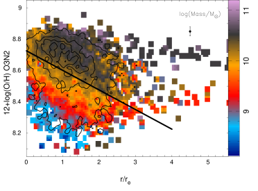
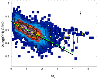
Figure 9: Left panel: Radial distribution for the oxygen abundance derived using the O3N2 indicator for all the galaxies in our sample. The contours show the density distribution of H ii regions in this parameter space. The outermost contour encircles 95% of the total number of H ii regions, with $\sim$20% less in each consecutive contour. The color image shows the average stellar mass of each galaxy corresponding to each abundance and radial distance. Right panel: Radial distribution for the oxygen abundance derived using the O3N2 indicator, after scaling to the average value at the disk effective radius for each galaxy. The image and contours show the density distribution of H ii regions in this parameter space. The outermost contour encircles 95% of the total number of H ii regions, with $\sim$20% less in each consecutive contour. The solid-yellow points represent the average oxygen abundances, with their corresponding standard deviations indicated as error bars for consecutive bins of 0.3 galactocentric distances per disk effective radius. The average error of the derived oxygen abundance (without considering systematic errors) is shown by a single error bar located a the top-right side of the panel. The dashed-green line shows the result of the best linear regression to the data. The solid-black lines in both panels represent the linear relation corresponding to the mean values of the zero-points and slopes of the individual regressions derived for distribution of each individual galaxy.

In Fig. 8, top-right panel, we show the distribution of slopes as a function of the galaxy morphological classification. This classification was performed by eye, based on the independent analysis by five members of the CALIFA collaboration, and it will be described elsewhere in detail (Walcher et al. in prep.). Different tests indicate that our morphological classification is fully compatible with pre-existing ones, and their results agree with the expectations based on other photometric/morphological parameters, like the concentration index (Fig 1) and/or the Sèrsic index (Sersic, 1968). We exclude from this analysis those galaxies with evidence of an on-going interaction (i.e., classes 1-5, in the previous section), since they present a much flatter gradient. This reduces our sample to 146 galaxies.

The earlier spirals (S0/Sa) present a slightly flatter slope, $\alpha_{O/H,S0-Sa}=-$0.08 dex/$r_{e}$ and $\sigma=$0.08 dex/$r_{e}$ ($n_{gal,S0-Sa}=$13), in comparison with the two groups of later type ones: $\alpha_{O/H,Sab-Sb}=-$0.12 dex/$r_{e}$ and $\sigma=$0.08 ($n_{gal,Sab-Sb}=$88) dex/$r_{e}$ and $\alpha_{O/H,Sbc-Sm}=-$0.11 dex/$r_{e}$ and $\sigma=$0.08 dex/$r_{e}$ ($n_{gal,Sbc-Sm}=$45). However, the corresponding $t$- and KS-tests indicate that the differences are not significant: $p_{t}=$98.86% and $p_{KS}=$81.31%, respectively, for the distributions with the larger differences. Therefore, statistically speaking, the slopes of spirals galaxies segregated by morphology are all equivalent.

A similar result is found if instead of normalizing the radial distances to the disk effective radius we adopt the physical size, without any scale-length normalization. In this case we derive a much wider distribution of slopes, not compatible with a Gaussian distribution (as indicated before). The only difference is that the values for the early-type galaxies are somehow shallower and with a narrower range than that of the later types, although the differences are not statistically significant.

4.2.3 Effects of bars in the abundance gradients

Fig. 8, bottom-left panel, shows the distribution of slopes for the different types of galaxies, depending on the clear presence, or not, of bars. The inspection of our sample for bars was performed by eye, by five members of the CALIFA collaboration, and it will be described elsewhere in detail (Walcher et al. in prep.). Three different groups were defined, following the classical scheme: (A) galaxies with no bar, (AB) galaxies that may have a bar, but it is not clearly visible and (B) clearly barred galaxies. The visual classification was cross-checked with an automatic search for bars, based on the change of ellipticity and PA, that has yield similar results. In a recent kinematical analysis of the H$\alpha$ velocity maps, using DiskFit, it was found that the frequency of radial motions was significantly higher in those galaxies with clear bars (Holmes et al., in prep.). As for the previous section, we only considered the 146 galaxies with no evidence of an on-going interaction.

Again, negligible differences in statistical terms are found between the slope of the abundance gradient for barred galaxies, i.e. $\alpha_{O/H,B}=-$0.09 dex/$r_{e}$ and $\sigma=$0.07 dex/$r_{e}$ ($n_{gal,S0-Sa}=$38), in comparison with the other two groups: $\alpha_{O/H,A}=-$0.12 dex/$r_{e}$ and $\sigma=$0.08 ($n_{gal,A}=$78) dex/$r_{e}$ and $\alpha_{O/H,AB}=-$0.13 dex/$r_{e}$ and $\sigma=$0.09 dex/$r_{e}$ ($n_{gal,AB}=$30). The corresponding $t$- and KS-tests indicate that the differences are not significant: $p_{t}=$93.43% and $p_{KS}=$92.44%, respectively, for the distributions with the largest differences. Therefore, if there is a change in the general slope of the gradient induced by the presence of a bar, the effect is weak and not statistically significant. The same result is found if the radial distances are normalized to the physical size, without any scale-length normalization. As in the previous case, we derive a wider distribution of slopes, but with no significant differences due to the presence or absence of bars.

4.2.4 Slopes by luminosity, stellar mass and concentration index

In the previous sections, we analysed the possible changes of the slope of the abundance gradient on the basis of three different morphological classifications: merging/interaction stage, Hubble type and incidence of bars. All those classifications were performed by eye, deriving a discrete segregation of the galaxies in sub-groups. In this section we analyse the possible variation of the slope as a function of less-subjective parameters, that are correlated with the morphology of the galaxies: the luminosity, the stellar mass and the concentration index $C$ (see definition in Sec. 2).

Fig. 8, bottom-right panel, illustrates this analysis, showing the distribution of slopes versus the $g$-band absolute magnitude of the galaxies. As in the previous sections we excluded the galaxies with clear interactions. We split the sample in luminous ($L$, M${}_{g}<=-$20.25 mag), intermediate ($I$, $-$20.25$<$M${}_{g}<=-$19.5 mag), and faint ($F$, M${}_{g}>-$19.5 mag) galaxies. No significant difference is found between both the average slopes: $\alpha_{O/H,L}=-$0.10 dex/$r_{e}$ and $\sigma=$0.08 dex/$r_{e}$ ($n_{gal,L}=$57), $\alpha_{O/H,I}=-$0.12 dex/$r_{e}$ and $\sigma=$0.06 dex/$r_{e}$ ($n_{gal,I}=$42), $\alpha_{O/H,F}=-$0.12 dex/$r_{e}$ and $\sigma=$0.10 dex/$r_{e}$ ($n_{gal,F}=$45). The corresponding $t$- and KS-tests indicate that the probability that they are different are $p_{t}=$88.11% and $p_{KS}=$87.36%, respectively, for the sub-samples with the largest differences. There is not even a weak trend between both parameters, given the derived correlation coefficient $r=$0.009, and a slope provided by a linear regression of $a=-$0.0007. Thus the abundance gradient seems to be independent of the luminosity of the galaxies.

Similar results are found for the stellar masses (derived as described in Sanchez et al., 2013), and the $C$-index. No clear correlation is found between the slopes of the abundance gradients and both parameters, as indicated by the derived correlation coefficients: $r_{mass}=$0.08 and $r_{C-index}=$0.24. The only difference is found for galaxies more massive than 4.5$\times$10¹⁰ M_⊙, with concentration indices larger than $C>$2.4 (34 galaxies). These galaxies present an average slope of $\alpha_{O/H}=-$0.07 dex/$r_{e}$ and $\sigma=$0.06 dex/$r_{e}$, and $t-$ and KS-tests indicate that they are significantly different from the rest of the sample: $p_{t}=$99.60% and $p_{KS}=$99.08%. However, even this difference has to be taken with care, since a visual inspection of the abundance gradients for this subsample indicates that a substantial fraction of them are galaxies with few detected H ii regions.

5 Discussion

The metal content of a galaxy is a fundamental parameter to understand the evolution of the stellar populations galaxy-by-galaxy and at different locations within the same galaxy. Oxygen is the most abundant heavy element in the Universe, making it the best proxy of total metallicity. It is easily observable for a wide range of metallicities thanks to its emissivity of collisionally excited lines, which are prominent in the optical regime. The existence of an universal radial decrease in the oxygen abundance has been already suggested in many previous studies (e.g. Diaz, 1989; Vila-Costas & Edmunds, 1992; Bresolin et al., 2009; Yoachim et al., 2010; Rosales-Ortega et al., 2011; Marino et al., 2012; Sánchez et al., 2012b; Bresolin et al., 2012). This observational property is compatible with our current understanding of the formation and evolution of spiral galaxies (e.g. Tsujimoto et al., 2010, and references therein). Gas accretion brings gas into the inner region, where it first reaches the required density to ignite star formation. Thus the inner regions are populated by older stars, and they have suffered a faster gas reprocessing, and galaxies experience an inside-out mass growth (e.g. Matteucci & Francois, 1989b; Boissier & Prantzos, 1999a). Several previous studies have analyzed the radial abundance gradients for individual galaxies or for limited samples of galaxies (e.g., Vila-Costas & Edmunds, 1992; Belley & Roy, 1992; Zaritsky et al., 1994; Roy & Walsh, 1997; van Zee et al., 1998; Marino et al., 2012; Rosales-Ortega et al., 2011; Rich et al., 2012; Bresolin et al., 2012). These studies have found: (i) a monotonic decrease of the abundance from the central regions, up to $r_{25}$ and/or $\sim$2.5 – 4 $r_{0}$ (the scale-length of the disk), which corresponds basically to $\sim$1.5 – 2.5 $r_{e}$; (ii) a flattening in the outer regions, for those galaxies that cover regions beyond $r_{25}$; (iii) in some cases a shallow drop of the abundance in the central regions is found (e.g. Rosales-Ortega et al., 2011, $<$0.3-0.5 $r_{e}$). In Sánchez et al. (2012b) we presented the first study of a large number ($\sim$2000) of H ii regions, extracted from 38 face-on spiral galaxies. In general, we confirmed the common pattern described above (although the sample of regions beyond $\sim$2$r_{e}$ was quite reduced), we found that there is not only a common pattern but a common slope of $\alpha_{O/H}=-$0.12 dex/$r_{e}$ for all the abundance gradients between 0.3-2.1$r_{e}$, when normalized to the disk effective radius of the galaxies.

The results presented in the previous section point to the same conclusion as Sánchez et al. (2012b), i.e., that independently of the large variety of analyzed galaxies, disk galaxies in the local Universe present a common/characteristic gradient in the oxygen abundance up to $\sim$2 disk effective radii. Moreover, the distribution around this mean value is compatible with a Gaussian function, and therefore could be the result of random fluctuations. This result contradicts several previous studies which claim that the slope in the gas-phase abundance gradient is related to other properties of the galaxies, such as (i) the morphology, with early-type spirals showing a shallower slope and late-type ones a sharper one (e.g. McCall et al., 1985; Vila-Costas & Edmunds, 1992), (ii) the mass, with more massive spirals showing a shallower slope and less massive ones a sharper one (e.g. Zaritsky et al., 1994; Martin & Roy, 1994; Garnett, 1998); and in particular, (iii) the presence of a bar, with barred galaxies presenting a shallower slope than non-barred ones (e.g. Zaritsky et al., 1994; Roy, 1996), and (iv) the interaction stage of the galaxies, with evolved mergers presenting shallower slopes (e.g. Rich et al., 2012), which seems to be the case also for irregular galaxies and low-mass galaxies (e.g. Edmunds & Roy, 1993; Walsh & Roy, 1997; Kobulnicky, 1998; Mollá & Roy, 1999; Kehrig et al., 2008).

In the first case, the dependence of oxygen abundance on the morphology of the galaxies is a long standing debate (e.g. McCall et al., 1985; Vila-Costas & Edmunds, 1992). Early results indicated that early-type spirals (S0/Sa) present flatter gradients than late-type ones (Sc/Sm), although these results were based on a handful of observed galaxies and it was never tested in an statistical sense, until the study presented here. Nevertheless, as described in Sec. 4.2.2, statistically speaking, the slopes of spirals galaxies segregated by morphology are all equivalent. In the case of the bars, it is well-known that at least a 30% of disk galaxies have a pronounced central bar feature in the disk plane and many more have weaker features of a similar kind (e.g. Sellwood & Wilkinson, 1993). Kinematic data indicate that the bar constitutes a major non-axisymmetric component of the mass distribution which tumbles rapidly about the axis normal to the disk plane. The theory predicts that bars are only stable inside co-rotation, although whether they are stable or not remains under discussion (e.g. Jogee et al., 2004; Méndez-Abreu et al., 2012). The bar and the spiral arms present two separate pattern speeds, with the bar rotating much faster, as has been recently observed (e.g. Pérez et al., 2012).

Bars have been proposed as an effective mechanism for radial migration (e.g. Di Matteo et al., 2013). Hydrodynamical simulations have shown that bars induce angular momentum transfer via gravitational torques, that result in radial flows and mixing of both stars and gas (e.g. Athanassoula, 1992). This radial movement can produce a mixing and homogenization of the gas, which leads to a flattening of any abundance gradient (e.g. Friedli et al., 1994; Friedli, 1998). Resonance patterns between the bar and the spiral pattern speed can shift the orbits of stars, mostly towards the outer regions (Minchev & Famaey, 2010), a mechanism that affects also the gas. Another process that produces a similar effect is the coupling between the pattern speed of the spiral arms and the bar that induces angular momentum transfer at the co-rotation radius (e.g. Sellwood & Binney, 2002a). Early observational results described a flattening in the abundance gradient of barred galaxies (Zaritsky et al., 1994; Martin & Roy, 1994). However, as first described in Sánchez et al. (2012b), and explained in Sec. 4.2.3 of this work, we found negligible differences in statistical terms between the slope of the abundance gradient for barred galaxies, i.e., no evidence of the claimed flattening.

A direct comparison between our derived slopes and those presented by previous results is dangerous, due to the inhomogeneity of the data. However, it is needed to investigate the source of the discrepancies. Zaritsky et al. (1994) presented an analysis of the abundance gradient based on a sample of 39 galaxies. Of them, 14 were new objects (comprising a total of 159 H ii regions), and the remaining ones were extracted from the literature. Finally, only 7 objects of the total sample present a clear bar. Although in general their abundance estimations cover a radial range up to $\sim$2 effective radii (or one isophotal radius in their nomenclature), in many cases the actual sampled spatial range is much more reduced (eg., NGC 1068 or NGC 4725, as can be seen in their Fig. 8). In other cases the slope is derived from a very low number of H ii regions (in particular some of the largest derived slopes), with values that have recently been updated to much smaller values (e.g., NGC 628, for which they derive a slope of $-$0.96 dex/$r_{25}$, when the actual value is 5 times lower, Sánchez et al., 2011; Rosales-Ortega et al., 2011; Sánchez et al., 2012b). Therefore the individual measurements presented in this article have to be taken with care, although they were most probably the best available at the time. Finally, the claim that barred galaxies present a flatter abundance gradient than non-barred ones is based on the comparison of this parameter for 7 barred with 32 non-barred galaxies (Fig.15 of that article). The strongest difference is found in the very late-type galaxies where there are just a few objects (3 barred and 3 non-barred galaxies, with Hubble Type T$>$6). Some of the reported values are hardly feasible, since slopes of $-$0.75 dex/$r_{25}$ could imply a range of abundances that is not observed across a galaxy in more recent estimations. On the other hand no distinction was made between interacting and non-interacting galaxies, which may introduce another source of uncertainty, since those galaxies present a flatter distribution (e.g. Rupke et al., 2010a, , and this study).

Martin & Roy (1994) presented a comparison of the abundance gradient based mostly on literature data. Of the 24 analyzed galaxies, they present new data for three barred galaxies, two of them with an apparent flatter abundance gradient than non-barred galaxies of the same morphological type (NGC 925 and NGC 1073). However, the slope they presented for those galaxies, when normalized by the effective radius, cannot be considered flatter than the average ($-$0.185 dex/$r_{e}$ and -0.254 dex/$R_{e}$, respectively, extracted from Table 7A,B from that article). Only when they compare the gradients of the barred and non-barred galaxies normalized to the physical scale (dex/kpc) can they find a difference, although they advise that ”the sample of each morphological type is small”. We have already indicated along this study the importance of defining the gradient normalized to the effective radius, since this parameter presents a clear correlation with other parameters of the galaxies, such as the absolute magnitude, the mass and the morphological type.

Their analysed sample comprises a heterogeneous selection of objects with the main criteria that they have at least 10 H ii regions with published abundance estimates in each galaxy. Of the 24 galaxies, nine have a large inclination angle ($>$55^∘, including NGC 925), and no inclination correction has been applied in the derivation of the abundance gradient. This may have an impact on the derived slopes. Finally, the three galaxies with flatter gradients ($=0$ dex/kpc) have been classified as merging systems, and two of them have been classified as barred galaxies. On the other hand, the galaxy with stronger gradient is also a merging system, being classfied as non-barred. If both highly inclined objects and merging systems are excluded from the comparison, there is no clear evidence of a difference between barred and unbarred galaxies in their sample.

The same result is found for the possible variation of the slope as a function of galaxy properties which are correlated with the morphology of the galaxies, i.e. the luminosity, the stellar mass and the concentration index $C$, as described in Sec. 4.2.4. When compared with previous literature data that described correlations with these parameters, we have to take into account how these results were derived (e.g. Zaritsky et al., 1994; Garnett, 1998), i.e., the analyzed sample of galaxies and H ii regions, and if they refer to the slope normalized to the physical scale or to a certain galactic scale-length. For example, Zaritsky et al. (1994), despite the caveats expressed before about their sample, found a correlation between the slope and different properties of the galaxies, such as the stellar mass, the rotation velocity and the morphological type, but only when the slope was expressed in terms of the physical size (dex/kpc). Since it is well-known that the effective radius of a galaxy correlates with those parameters, both results may be compatible, as suggested already in Sánchez et al. (2012b).

Finally, it is important to remember that in many cases well established results are based on reduced and heterogenous samples of galaxies with an insufficient number of H ii regions explored, or with comparison samples also extracted from literature data. Berg et al. (2013) explain that most old estimates of radial gradient of oxygen abundances in the literature are based on out-of-date strong-line empirical calibrations which may be uncertain. These authors measure the auroral line [O iii]$\lambda$4363 and find a gradient of -0.017 dex/kpc and -0.027 dex/kpc for NGC 638 and NGC 2403, respectively, which correspond to -0.10 and -0.15 dex/$r_{e}$ in perfect agreement with results. These values are much smaller than the old ones, as also occurs with the estimates from Bresolin (2011) and Bresolin et al. (2012) for M 33, M 31, NGC 4258 and M 51, which are now -0.042, -0.023, -0.011 and -0.020 dex/kpc, smaller than the old numbers reported by Zaritsky et al. (1994). In fact the value of -0.017 dex/kpc for NGC 628 is very similar to the one found by Rosales-Ortega et al. (2011), as indicated before (compatible with the value reported by Berg et al., 2013). Therefore the procedure to measure the gradient is important, as well as the number of points or other important observational effects, such as the angular resolution, the signal to noise, or the annular binning that may also change the obtained radial gradient, such as it is demonstrated in Yuan et al. (2011) and Mast et al. (in prep.).

In the case of the effects of interactions on the abundance gradient of galaxies, theory predicts that major mergers trigger the formation of bars in the stellar and gas disks, which induce vigorous gas inflows as the gas looses angular momentum to the stellar component (Barnes & Hernquist, 1996). These in-flows are thought to be responsible for fueling a massive central starburst and feeding AGN and/or quasar activity (Mihos & Hernquist, 1996; Barnes & Hernquist, 1996). For a spiral galaxy with a preexisting metallicity gradient, gas in-flow flattens the gradient by diluting the higher abundance gas in the central regions with the lower abundance gas from the outer parts (Rupke et al., 2010a, b; Kewley et al., 2010). This flattening is compounded as the spiral arms are stretched by tidal effects (Torrey et al., 2012). In addition, interactions induce central star formation processes that produce violent outflows that eject metals from the richer central regions (e.g., Wild et al., in prep.). Indeed, galaxy mergers and interacting systems seem to present flatter gradients in the oxygen abundance (e.g. Kewley et al., 2010; Rich et al., 2012). The results of Sec. 4.2.1 support the same scenario, i.e., that galaxy interactions flatten the abundance gradient of spiral galaxies in a statistical sense.

5.1 The common abundance gradient

The results of the present study indicate that, when using the O3N2 strong-line abundance indicator, the oxygen abundance gradient in disk galaxies present, statistically, a common slope of $\sim-$0.1 dex/$r_{e}$, between 0.3 and 2.1 disk effective radius, when normalized to this disk effective radius. This common slope is independent of the other properties of the galaxies, except for interaction/merging and maybe for the more massive and concentrated galaxies.

Following Sánchez et al. (2012b) it is possible to illustrate this result by presenting the radial distribution of the oxygen abundance for all the galaxies in a single figure. Since the representative abundance (i.e., the abundance at the disk effective radius) scales with the integrated mass (Sanchez et al., 2013), following the well known $\mathcal{M}$-Z relation (Tremonti et al., 2004), it is required to apply a global offset galaxy by galaxy, and normalize the gradient by the mean value at the disk effective radius for all the sample, i.e., 12 + log(O/H) = 8.6 dex. Figure 9 illustrates this process. In the left panel, we show the contour-plot of the radial distribution before re-scaling to the average representative abundance. The distribution comprises $\sim$4500 H ii regions corresponding to 193 different galaxies of any morphological type, including barred and un-barred galaxies, and covering all the CM-diagram to the completeness limit of the CALIFA survey (described in Walcher et al. in prep.). Although the radial gradient is still visible, there is a wide distribution that almost blurs the evidence of a common abundance gradient. The color-coded areas represents the integrated stellar mass of each galaxy corresponding to each represented abundance (in log units). As expected from the $\mathcal{M}$-Z relation, for an equal mass the abundances present a clear radial gradient, parallel to the average of the individual linear regressions derived for each galaxy (solid-line), up to $\sim$2 disk effective radii. This figure illustrates clearly that the common gradient is independent of the mass, as mentioned in previous sections.

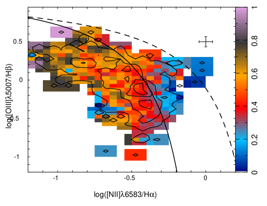
Figure 10: BPT diagnostic diagram similar to the one presented in Fig. 4, right-panel, restricted to the H ii regions beyond 2.2 disk effective radius. The contours indicate the number density of regions, while the color-coded image represent the fraction of young stars ($<$500 Myr). The error bar represents the typical error in both parameters for the represented H ii regions.

The right-panel of Fig. 9, shows the average radial distribution of the oxygen abundance after re-scaling to the average representative abundance. The distribution of H ii regions is represented as a density map, both with a color-coded image and a contour map (with the first contour encircling 95%) of the regions. The solid-yellow circles indicate the mean abundances at equal spatial bins of $\Delta r=$0.3 r_e with the error bars indicating the corresponding standard deviation. No significant deviation from the monotonic decrease defined by the average gradient (represented with the black solid line), is found up to 2.1 disk effective radii. A linear regression to the scaled distribution of H ii regions, restricted to the spatial range between 0.3 and 2.1 r_e (represented by the green dashed-line) derives a slope of $\alpha_{O/H}-$0.107 dex/$r_{e}$ and $\sigma=$0.004 dex/$r_{e}$, fully compatible with the average value found for all the sample $\alpha_{O/H}-$0.09 dex/$r_{e}$ and $\sigma=$0.09 dex/$r_{e}$ (solid black line).

The origin of this common abundance gradient has to be directly linked to the formation and evolution of the disk in spiral galaxies. Recent results, based on the analysis of the star-formation history of CALIFA data, found undisputed evidence of the inside-out growth of the stellar mass in galaxies (Pérez et al., 2013), at least for galaxies more massive than 7$\times$10¹⁰ M$\odot$. Both the extinction-corrected color gradients in nearby galaxies (Muñoz-Mateos et al., 2007), and weak dependence on the mass-size relation with redshift (Trujillo et al., 2004; Barden et al., 2005; Trujillo et al., 2006) also support an inside-out scenario for the evolution of disks. These results are also supported by the radial distribution of the stellar ages found for the same data set (González Delgado et al., 2013).

However, the described universal slope for the abundance gradient, being independent of many of the properties of the galaxies, was only recently described (Sánchez et al., 2012b). This result imposes a more severe restriction to our current understanding of how disk galaxies grow. In essence, it agrees with the recently proposed $\Sigma$-Z relation (Rosales-Ortega et al., 2012), that links the gas abundance with the mass density of the underlying stellar population. It describes how the stellar mass and the gas abundance, both fundamental products of the star formation history, grow side-by-side in disk galaxies, from the center to the outer-parts. Together with the $\mathcal{M}$-Z relation, they indicate that more massive galaxies (that trace the deepest potential-wells), form before and faster, accumulating more stellar mass and more metals. The presence of a common gradient in the abundance indicates that all disk dominated galaxies of the same disk effective radius (hence, same disk mass, if having similar central surface brightness) synthesize metals at the same galactocentric distance with a similar efficiency.

The common slope suggests that the chemical evolution of galaxies is very similar in all disk galaxies, being compatible with a pseudo closed-box model. The classical closed-box model considers that each radial bin of a galaxy comprises primordial gas from which stars are born, live all their life-time and die in-situ, according to a given SFR and IMF prescriptions (Pagel & Patchett, 1975). Therefore, if the amount of primordial gas is proportional to the depth of the potential well, and the efficiency of the SFR is the same for all the galaxies, both the stellar mass and the enrichment would only be proportional to the time, for a given halo mass. The efficiency of the SFR (or starformation efficiency, SFE), is defined as the SFR surface density per unit of neutral gas surface density along a line of sight. Recent results indicate that the SFE does not vary strongly where the ISM is mostly H₂, in spiral galaxies (e.g. Leroy et al., 2008). Under this assumption all galaxies should have an universal gradient of their oxygen abundance with its zero-point proportional to the total mass.

However, it is well known that the closed-box model cannot predict the right fraction of metal-poor stars with respect to the observed metallicity distribution of nearby long-lived stars in the Milky Way (e.g. Gibson et al., 2003). A more realistic model overcomes this problem by allowing the disk of galaxies to form via continuous accretion of gas, driven by the gravitational force (pseudo closed-box model). This accretion can be compensated or even halted for certain galaxies and over certain periods by supernova explosions (e.g. Larson, 1974). However, the outflow of gas is not expected to feature in the history of most spiral galaxies and is usually neglected in the models (Gibson et al., 2003). This modified model is consistent with the described common radial gradient if the local gas recycling is faster than other timescales involved (Silk, 1993), and if the radial inflow is similar for those radial bins with the same stellar mass.

In summary, the radial gradient appears to be the consequence of different evolutionary rates along the radius. Recent chemical evolution models suggest that the inner regions evolve faster than the outer ones (Mollá & Díaz, 2005), following a local downsizing evolution in agreement with the $\Sigma$-Z relation Rosales-Ortega et al. (2012); Sanchez et al. (2013). Therefore, an evolution in the slope of the radial gradient expressed in physical scales (dex/kpc) is expected, with a flattening for the more massive or more evolved galaxies (Mollá & Díaz, 2005). The described characteristic slope of the radial gradient when normalized to the effective radius (dex/$r_{e}$) implies a tight co-evolution of the radial gradient with the scale-length of the galaxy, with more massive galaxies being larger (which is also observed).

5.2 The flattening of the abundance gradient in the outer regions

The linear regressions shown in the right-panel of Fig. 9 have been extrapolated beyond r$>$2.2 effective radii to illustrate the fact that in the outer regions the abundances present a clear flattening, as already shown in Fig. 5 for some individual galaxies. We detected 484 H ii regions at these outer areas, corresponding to 94 individual galaxies. In most of them the derived abundance is larger than the expected by the extrapolation of the monotonic decrease.

Average radial distributions of oxygen abundances, similar to the one shown in Fig. 9, were created for different subsamples of galaxies, segregated by their morphology, photometric properties and the structural parameters. The same subgroups analysed in the previous section where selected. No significant difference is found in either the qualitative and quantitative shape and slope of the radial gradient. It is worth noting that the flattening at the outer regions seems to be a universal property of disk galaxies, independent of the inclination, mass, luminosity, $C$-index, morphology and/or presence of bars. Only in the case of the interacting galaxies, with a much lower slope in the abundance gradient in the inner disk it is unclear whether or not an outer flattening exists (or if all the distribution is flattened). It is also important to bear in mind that although we have adopted the O3N2-indicator, the flattening does not depend on the actual strong-line indicator selected. We tested it using the R23-based calibrator by Tremonti et al. (2004), the N2-based calibrator by Pettini & Pagel (2004) and the C-method described by Pilyugin et al. (2012), with consistent results.

As mentioned before, several previous studies found a similar behavior for individual or a limited sample of galaxies (e.g. Bresolin et al., 2009; Yoachim et al., 2010; Rosales-Ortega et al., 2011; Marino et al., 2012; Scarano et al., 2011; Bresolin et al., 2012). We have found a first hint of this flattening in our pilot analysis of the face-on galaxies in the CALIFA feasibility sample plus PINGS data, for a limited set of galaxies and H ii regions (Sánchez et al., 2012b). The same pattern in the abundance was described (i) in the extended UV disks discovered by GALEX (Gil de Paz et al., 2005; Thilker et al., 2007); (ii) in the metallicity gradient of the outer disk of NGC 300 from single-star CMD analysis (Vlajić et al., 2009), (iii) in the Milky-way, based on the spectroscopic analysis of the outer H ii regions (Vilchez & Esteban, 1996; Esteban et al., 2013), using open clusters (e.g. Bragaglia et al., 2008; Magrini et al., 2009; Yong et al., 2012), or Cepheids (e.g. Andrievsky et al., 2002; Luck et al., 2003; Andrievsky et al., 2004; Lemasle et al., 2008); and (iv) in the oxygen abundance gradient of different individual galaxies, like M 83 (Bresolin et al., 2009), NGC 628 (Rosales-Ortega et al., 2011), or NGC 1512 and NGC 3621 (Bresolin et al., 2012), to cite just a few results. However, this is the first unambiguous detection of such a flattening in most of the galaxies with detected H ii regions beyond $\sim$2 effective radii.

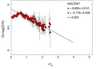
Figure 11: Radial distribution of the oxygen abundance derived for the individual H ii regions for NGC 2347, one of the galaxies showing a clear drop of this parameter in the inner regions. The symbols, lines and labels are the same as the ones shown in Fig. 5.

The nature of this flattening is still under debate, in particular because until the current study it was not even clear if it is a common feature of all disk-galaxies. The observational and theoretical investigations of the metal content in the outer regions of galaxies is relatively recent. Because of their extreme conditions (e.g. very low gas densities and long dynamical timescales), the outermost regions of the galaxies are sensitive probes of the mechanisms leading to the assembly of the disks and their evolution, and thus of great importance for constraining galactic chemical evolution models. The flat abundance distribution in the outer regions of galaxies corresponds usually to the lowest metallicity values in the galaxies. Nevertheless, these abundances are still relatively high. Assuming continuous star formation with the currently observed SFR, the time required to enrich the ISM up to 12 + log(O/H) $\sim 8.2$ has been estimated in $\sim 10$ Gyr. (Bresolin et al., 2012). According to cosmological hydrodynamic simulations, in the inside-out scenario for galaxy growth the outer disks of galaxies are formed in the last $\sim 4-6$ Gyr. (Scannapieco et al., 2008, 2009), making unlikely that the in situ star formation could have enriched the interstellar medium to the presently observed values. Therefore, in the case of isolated galaxies, alternative mechanisms of metal redistribution must play an important role.

Among the different proposed processes that could produce this abundance flattening we wish to mention: (i) large-scale processes of angular momentum transport that produce an intermix of gas abundances, including radial gas flows (e.g. Lacey & Fall, 1985b; Goetz & Koeppen, 1992b; Portinari & Chiosi, 2000; Schönrich & Binney, 2009; Spitoni & Matteucci, 2011), resonance scattering with transient spiral density waves (Sellwood & Binney, 2002b), and the overlap of spiral and bar resonances (Minchev et al., 2011); (ii) minor-mergers, and captures of, or perturbations by satellite galaxies that increase the metal content in the outer regions (Quillen et al., 2009; Bird et al., 2012); (iii) a non linear Schmidt-Kennicutt law that is able to trigger highly efficient star-formation process at these distances (e.g. Esteban et al., 2013); (iv) a spatial association of the flatter area with gas located in the thick disk, which is known to have different metallicity patterns (e.g. Neves et al., 2009; Ishigaki et al., 2012); (v) a plateau of the gas abundance in the intergalactic medium due to the cosmological evolution of galaxies, and the subsequent pollution of metals (Sánchez et al., in prep.); etc. Stellar radial migration has also been proposed as a possible cause for the flattening of the metallicity gradients for stellar populations in spiral galaxies (e.g. Roškar et al., 2008b, a). However, this argument is valid only if stars and gas are not decoupled.

The detailed understanding of the nature of the flattening will require further observational and theoretical efforts. However, we can outline some of the properties of the H ii regions in this regime, that may help to constrain and distinguish between the different scenarios summarized before. Figure 10 shows the BPT diagram for the 484 H ii regions beyond 2.2 disk effective radii, together with the fraction of young stars corresponding to each region, as presented in Fig.4. Although the number of regions here is more limited than the whole sample, the distribution as a function of the BPT diagram is very similar. It shows a clear gradient in the stellar populations, covering a range of young stars of almost a 100% to nearly $\sim$30%. The range of oxygen abundances measured in these regions is 8.2$<$12 + log(O/H)$<$8.7. Thus, based on the analysed parameters these regions do not show clear differences with respect to the remaining population at small galactocentric distances.

As indicated before, even at these galactocentric distances it is possible to find H ii regions located above the Kauffmann et al. (2003) curve ($\sim$15% beyond 2.2 effective radii). Due to their galactocentric distance, these regions cannot be contaminated by a non-negligible possible central ionizing source (like an AGN), and the diffuse emission is also extremely weak to affect the line ratios. A visual inspection of the H$\alpha$ maps reveals that they are bona fide H ii regions, as can be appreciated in Fig. 2 and Fig. 5 for the case of UGC 312. This result reinforces our adopted selection criteria, i.e. by using the information of the underlying stellar population as a proof for on-going star-formation activity, we do include H ii regions that would otherwise be discarded by using solely empirical demarcation curves based on strong emission-lines, like the Kauffmann et al. (2003) curve.

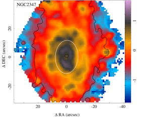
Figure 12: Color-coded image of the H$\alpha$ intensity flux, in logarithmic scale of 10^-16 erg s^-1 cm^-2 arcsec^-1units , corresponding to NGC 2347 (the galaxy shown in Fig. 11). The contours represent the flux intensity in the V-band, extracted from the datacube the datacube, at two intensity levels, 0.2 10^-17 erg s^-1 cm^-2 arcsec^-1 (corresponding to $\sim$3 $\sigma$ detection limit in the continuum) and 15 10^-17 erg s^-1 cm^-2 arcsec^-1, included to illustrate the location of the center of the galaxy. The white ellipse indicates the location of the knee/peak in the radial abundance shown in Fig. 11.

5.3 Abundance decrease in the inner regions

Some galaxies present a truncation in the monotonic increase of the oxygen abundance towards the center, or even a drop in the inner regions, at $\sim$0.3-0.5 $r_{e}$ (e.g. Rosales-Ortega et al., 2011; Sánchez et al., 2012b). In the Milky Way, the metallicity distributions in the Galactic bulge, in the nuclear bulge and in the Galactic bar display different trends and are difficult to assess given the obvious geometrical obstacles. However, iron abundance determinations using stellar tracers (WR, luminous blue variables, red supergiants) located along the Galactic bar and in the nuclear bulge are more metal-poor than classical Cepheids in the inner disk, suggesting that the metallicity distribution is probably approaching a plateau toward the shortest Galactocentric distances ($R_{G}<5.5$ kpc, [Fe/H] $\sim$0.4 Genovali et al., 2013, and references therein). This flattening has been observed in other galaxies apart from the Milky Way (e.g. Werk et al., 2011; Bresolin et al., 2012; Sánchez et al., 2011) and has been predicted by some chemical evolution models (e.g. Mollá & Díaz, 2005, Molla et al., 2013, submitted). In some galaxies, such as NGC 628, the decrease was associated with a starforming ring, with a clear signature in both the H$\alpha$ emission and the underlying stellar population (e.g. Wakker & Adler, 1995; Ganda et al., 2006; Fathi et al., 2007; Sánchez et al., 2011). This circumnuclear ring was placed at the expected location of the inner Lindblad resonance, where gas is expected to accumulate due to non-circular motions (Fathi et al., 2007). Despite this possible explanation, it is not known if this is a common feature of all galaxies or, on the contrary, characteristic of a physically distinct galaxy subclass.

In Sánchez et al. (2012b), we found that the drop in the inner region was present in a substantial fraction of the galaxies, and it was visible in the average gradient. Figure 9, right-panel, shows the common abundance gradient for our current sample, which comprises many more galaxies and was properly selected to be statistically significant (Walcher et al., in prep.). There is no evidence for the a central drop in the average gradient, indicating that it is not a common feature of all the galaxies.

We perform a visual inspection of the individual gradient of each galaxy, classifying them as (i) objects without evidence of an inner drop in the abundance (146); (ii) objects with a possible evidence of a drop (21); and (iii) objects with a clear evidence of a drop (26). Figure 11 shows the typical abundance gradient of this latter case, corresponding to NGC 2347. The galactocentric distribution shows a monotonic, linear gradient from $\sim$0.6 to $\sim$2.4 disk effective radius, with a hint of a flattening beyond this radius, and a clear drop in the central regions ($<$0.6 $r_{e}$). We should note here that “drop” is used as a general term, defining either a real negative gradient towards the center or just a flattenning in the inner regions. The number of detected H ii regions and the error associated with their corresponding abundances prevent us from making a firm distinction.

Half of these galaxies are morphologically classified as Sb/Sbc (13 out of 26), although a KS-test of the morphological distribution compared with the corresponding one for the full sample (or the sample without evidence of a drop), indicates that both samples are not significantly different. The same result is derived when using the galaxies with possible evidence of an inner drop. Therefore, the drop does not seem to be associated with a particular morphological type of galaxies.

As we mentioned before, bars may induce radial motions of gas and stars, which may produce the described effect either by a mix of the gas content inside the bar length or by a transfer of gas towards the edge of the bar. Cavichia et al (2013, submitted) have developed a chemical evolution model in which the bar is taken into account in driving a radial flow outwards or towards the inner regions. With this model a slight flattening of the radial gradient of abundances appears along the disk, but only in the bulge-disk interface region. Thus, at the corotation radius of the bar there is an increase of SFR and, in consequence, the oxygen abundance increases. The net effect is that there is an apparent decrease or drop of the abundance in the central regions when actually there is a hump around 0.5$r_{e}$. If a bar were the dominant effect that produces the decrease of abundance in these galaxies, then it would be expected to detect it more frequently in barred galaxies. However none of these effects are observed. Although the sample is still too small to provide a statistical significant statement, the fraction of barred galaxies within the galaxies with clear drop of the abundance in the inner areas ($\sim$15%, 3 out of 21, once excluded the edge on galaxies) is half of the observed for the total sample ($\sim$28%, i.e., 53 out of 193).

As we indicated in Sec. 4.2.1, interactions and mergers are events that may produce also a change in the distribution of abundances in galaxies, due to radial motions induced by changes in the angular momentum patterns. We speculate that these kind of disturbances may also induce the detected drop of abundances in the inner regions of galaxies (e.g. by a minor-merger or a satellite galaxy capture). However, when analyzing the interaction stage of our sub-sample of galaxies with an inner drop we found that none of them presents some evidence of an on-going interaction/merging event. Therefore, it seems that this effect is due to the secular evolution of the galaxy, and not induced, in general, by the presence of an on-going interaction (although it does not discard past interactions or a minor merger that are not evident in the morphology of the galaxies).

If the origin of the drop is due to radial movements of the gas, then its presence would also have an effect on the overall distribution of abundances at larger radii. In order to explore if the presence of an inner drop has any effect in the determination of the slope of the abundance gradients (measured between $0.3-2.1$ disk effective radii), we performed the following test: if we only consider the slopes of the abundance gradients for the galaxies with clear evidence of a drop, we obtain a mean slope $\alpha_{O/H,drop}=-$0.15 dex/$r_{e}$ and $\sigma=$0.06 dex/$r_{e}$ (26 objects), which is significantly larger than the slope for the galaxies without evidence of such a drop, i.e. $\alpha_{O/H,drop}=-$0.08 dex/$r_{e}$ and $\sigma=$0.08 dex/$r_{e}$ (146 objects), with a probability of being different of $p_{KS}=$99.86%. This is consistent with a radial movement towards the knee/peak point in the abundance distribution, outwards from the inner regions and inwards from the outer ones.

A detailed inspection of the H$\alpha$ intensity maps of the less inclined galaxies shows that in most of them there is a star-forming ring that is spatially located inside the galactocentric distance defined by the knee in the radial distribution of the abundance. Figure 12 shows an example of this ring detected in the H$\alpha$ distribution of NGC 2347. A similar result was found for NGC 628 (Sánchez et al., 2011), using data with better physical spatial sampling provided by the PINGS survey (Rosales-Ortega et al., 2010). We speculate that the presence of the circular star-formation ring and the drop in the oxygen abundance inwards (together with the lack of evidence of an interaction and the low fraction of barred galaxies with these features), suggest that both features are the consequence of gas radial motions induced by resonances in the disk-speed pattern (Roškar et al., 2008b).

We will explore this hypothesis in the future with a detailed analysis of the stellar and gas kinematics, using the V1200 data available for the CALIFA objects.

6 Conclusions

In this article we described the procedures to detect, select, and analyse the spectroscopic properties of the largest homogeneous catalog of H ii regions and associations observed to date. This catalog comprises more than 5000 ionized regions associated with star-formation distributed in 227 galaxies of different morphological types, and evenly distributed along the color-magnitude diagram (out of 306, that comprised our original sample). We demonstrated that the combination of the properties of the ionized gas with the on-going underlying stellar population provides a robust means for selecting bona fide H ii regions, without excluding regions that would had been disregarded by other classical methods.

We use strong-line indicators to derived the oxygen abundance, and the deprojected galactocentric distances to derive the radial distances of the individual H ii regions. With this information we explore the radial abundance gradients for the individual galaxies in our sample. The results of this paper show that disk galaxies in the local Universe present a common or characteristic gradient in the oxygen abundance of $\alpha_{O/H}=-$0.1 dex/$r_{e}$ up to $\sim$2 disk effective radii, with a small dispersion compatible with being produced by random fluctuations. No significant differences are found on the basis of the morphological type, presence or absence of bars, absolute magnitude and/or stellar mass. A weak trend towards slightly flatter gradients is found for massive ($>$4.5 10¹⁰ M$\odot$) and highly concentrated galaxies ($C>$2.4), although there are galaxies with few number of H ii regions and with the less clearly defined disk. The only clear deviation from the common slope is seen in galaxies with evidence of interaction or undergoing merging. For these galaxies the gradient is significantly flatter. Similar results are obtained with other normalization radii than $r_{e}$, like the disk scale-length ($r_{d}$) or the radius at which the surface brightness reaches 25 mag/arcsec² ($r_{25}$). The use of different normalization radii only changes the numerical values of the common slopes.

These results agree with the main conclusions of our previous study (Sánchez et al., 2012b), where a limited sample of 38 face-on spiral galaxies was analysed, using similar methods as the ones described here. Both results apparently contradict previous works, in which the slope of the radial gradients show a trend with certain morphological characteristics of the galaxies. Vila-Costas & Edmunds (1992) and Zaritsky et al. (1994) showed that barred spirals have a shallower gradient than non-barred ones. However, we must recall here that these statements are based (in general) on gradients constructed on physical/linear scales (i.e. dex kpc^-1), not on normalized ones (see Appendix B for a discussion on the dependence of the results on the normalization). A slight decrease in the scatter between the different slopes is found by Vila-Costas & Edmunds (1992) and Diaz (1989), when the scale-length is normalized by the disk-scale, which agrees with our results. We conjecture that both results would come into agreement if the size-luminosity/morphological type relation was considered. In a companion article (Sánchez-Blázquez, in prep.), we analyse the radial gradient of stellar metallicity, where we have found consistent results, i.e. when normalized to the effective radius of the disk, the slope of the stellar population gradients does not correlate with the mass or with the morphological type of the galaxies, we do not find any difference in the metallicity or age gradients in galaxies with and without bars, and the young stellar population shows a metallicity gradient which is very similar to that of the gas.

We argue that the common slope suggests that the chemical evolution of galaxies is very similar in all disk galaxies, being compatible with a “modified” closed-box model, in which the disk of galaxies form via continuous accretion of gas, driven by the gravitational force. In this scenario, if the amount of primordial gas is proportional to the depth of the potential well, and the efficiency of the SFR is the same for all the galaxies, both the stellar mass and the chemical enrichment would be just proportional to the time, for a given halo mass. Under this assumption all galaxies should have an universal gradient of their oxygen abundance with its zero-point proportional to the total mass. It is important to note that our results do not deny the existence of radial movements and metal mixing, although they put new constraints on their net effects on the properties of the galaxies.

Galaxies under interaction or undergoing a merger event show a clearly flatter oxygen abundance distribution, in agreement with recent results by Kewley et al. (2010) and Rich et al. (2012). This indicates that these dynamical processes can produce an effective mixing of metals. On the contrary, the fact that barred and unbarred galaxies do not present a clear difference in their abundance slope indicates that bars either (i) do not significantly enhance the efficiency of chemical mixing; (ii) they produce a proportional change in the gas abundance and stellar mass distributions, which compensate each other when normalized by the disk effective radius or (iii) they are of temporary nature with a life-time that is shorter than chemical mixing timescale.

Another conclusion reached by this study is that the flattening of the abundance gradient at the outer regions seems to be an universal property of disk galaxies. Beyond $\sim$2 disk effective radii, our data shows a clear evidence of a flat distribution of the oxygen abundance in most of the galaxies with detected H ii regions at these radial distances. This feature has been previously reported by several authors (e.g. Bresolin et al., 2009; Marino et al., 2012; Bresolin et al., 2012; Sánchez et al., 2012b), although with less significant numbers. Although we cannot provide a conclusive answer regarding the origin of this flattening, our results suggest that its origin is most probably related to the secular evolution of galaxies, involving processes like radial migration, or the capture of evolved satellite galaxies. On the other hand, it disfavors other scenarios, such as a change in the efficiency of the star formation or the accreation of chemically polluted intergalactic media. Further analysis is required to provide a better understanding of this effect.

Finally, we also present observational evidence for a decrease of the oxygen abundance in the central region of some particular galaxies. Our analysis indicates that this drop is associated with central star-forming rings. A plausible explanation would be that both features are produced by the radial flow of gas induced by resonances in the disk pattern speed. The slightly increase of the slope beyond the knee/truncation point of the oxygen abundance, the lack of this feature in interacting systems, and the fact that it is more frequent in non-barred galaxies support this scenario.

Appendix A Effective radius of the disk

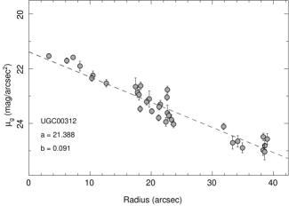
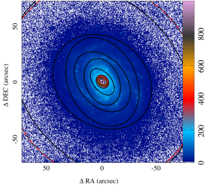
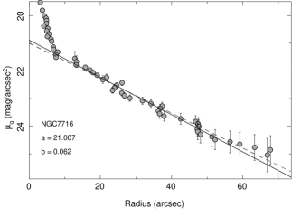
Figure 13: Left-panels: Color-scale representation of 1.5$\arcmin$$\times$1.5$\arcmin$ postage-stamp images extracted from the SDSS $g$-band data (in counts), centred in two CALIFA targets (UGC 00312 and NGC 7716), together with a set of ellipses (solid-black lines) representing the recovered shape at different isophotal intensity levels by the analysis described in the text. The last dashed red-black ellipse represents the 1$\sigma$ isophotal intensity level over the background, adopting the median ellipticity and position angle to plot it. Right-Panel: Surface brightness profiles derived for the considered galaxies on the basis of the corresponding isophotal analysis (gray solid circles), together with the best fit to an exponential profile for the portion of the surface brightness dominated by the disk (gray dashed line). For NGC 7716 a previous iteration of the fitting procedure is shown, before the rejection of those values dominated by the bulge (solid-line).

In Sánchez et al. (2012b) we showed that the abundance gradient of the analyzed galaxies presents a common gradient up to $\sim$2 $r_{e}$, when normalized to the effective radius of the disk ($r_{e}$). To repeat the same analysis for the CALIFA dataset included in this study, in addition to the abundances of the individual H ii regions, we need to derive this structural parameter for each galaxy.

The effective radius of the disk was derived based on an analysis of the azimuthal surface brightness profile (SBP). To derive the SBP, we perform an isophotal analysis of the ancillary $g$-band images collected for the CALIFA galaxies (extracted from the SDSS imaging survey, York et al. 2000, and Paper I).

These images were created using the SDSSmosaic tool included in IRAF (Zibetti et al. 2009). SDSSmosaic takes the galaxy coordinates as input argument and downloads all the individual SDSS frames and the photometric information from the SDSS DR7 web site for all 5 bands. These frames are then stitched together, accurate astrometry is computed and the photometric calibration is written into the header. After that, the background is subtracted from each scan by fitting a plane surface (allowing for linear gradient along the scan direction, constant in the perpendicular direction) outside a circle centered on the source. Finally, stripes are combined in a mosaic using the program Swarp (Bertin et al. 2002). The final mosaic contains the photometric zero point (P_ZP keyword) in mag per second of exposure time (EXPTIME keyword). We extracted postage-stamp images of 3$\arcmin$$\times$3$\arcmin$ size, centred in the CALIFA targets, for the $g$-band mosaic images to derive the disk effective radius.

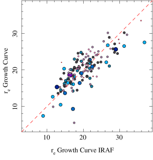
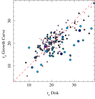
Figure 14: Left panel: Distribution of the effective radius of the analysed galaxies, derived from a growth curve analysis (i.e., the total light effective radius), as a function of the same effective radius derived by a similar growth curve analysis using the surface-brightness profiles derived using the ellipse task in IRAF. Right panel: Distribution of the effective radius of the analysed galaxies, derived from a growth curve analysis (i.e., the total light effective radius), as a function of the effective radius of the disk, derived from the exponential fitting to the surface brightness profile. In both panels, larger and bluer symbols correspond to earlier-type galaxies, while smaller and pinky/reddish ones correspond to later-type galaxies.

The isophotal analysis was performed using the ellipse_isophot_seg.pl tool included in the HIIexplorer package). Contrary to other tools, like ellipse included in IRAF, this tool does not assume a priori a certain parametric shape for the isophotal distributions. The following procedures were followed for each postage-stamp image: (i) the peak intensity emission within a certain distance of a user defined center of the galaxy was derived. Then, any region around a peak emission above a certain fraction of the galaxy intensity peak is masked, which effectively masks the brightest foreground stars; (ii) once the peak intensity is derived, the image is segmented in consecutive levels following a logarithmic scale from this peak value, using the equation:

$${\rm seg(i,j)=\leavevmode\nobreak\ n_{levels}\frac{log_{10}\leavevmode\nobreak\ flux(i,j)}{log_{10}\leavevmode\nobreak\ flux_{peak}}}$$ (5)

where seg(i,j) is the final segmented index at the pixel (i,j), being an integer number; n_levels is the number of selected levels of the isophotal analysis (100 in our case); flux(i,j) is the intensity at the corresponding pixel (i,j) and flux_peak is the peak intensity at the center of the galaxy; (iii) once the image is segmented in $n_{levels}$ isophotal regions, for each of them, a set of structural parameters was derived, including the mean flux intensity and the corresponding standard deviation, the semi-major and semi-minor axis lengths, the ellipticity, the position-angle and the barycenter coordinates. These parameters are intended to describe each isophote following an elliptical shape, but without performing direct fit, which is in principle more stable in lower signal-to-noise regimes. Figure 13, left panels, illustrates the process, showing for two particular objects a central section of 1.5$\arcmin$$\times$1.5$\arcmin$ of the postage-stamp images used in this analysis, together with a set of ellipses plotted using the recovered shape parameters for some particular isophotes.

The isophotal segmentation (2nd step of the described procedure), was first introduced by Papaderos et al. (2002). Noeske et al. (2003) and Noeske et al. (2006) showed that the surface-brightness profiles derived using this technique were very similar to those derived using more broadly adopted techniques, like the 2D GALFIT code (Peng et al. 2002). We have adopted this isophotal annuli procedure in previous studies, e.g. Kehrig et al. (2012), Papaderos et al. (2013) and Mast et al. (submitted). The improvement with respect to a pure isophotal segmentation was the additional derivation of the structural parameters for each isophotal region, described before (step iii).

The isophotal analysis provides a SBP, which is then analyzed to derive the required effective radius. Figure 13, right panels, show two examples of the derived SBPs for those galaxies shown in the left panels. In (Sánchez et al. 2012b), where all the galaxies were clearly disk-dominated, the profiles were fitted using a pure exponential profile, following the classical formula,

$$I=I_{0}\exp[-(r/r_{d})]$$ (6)

where $I_{0}$ is the central intensity, and $r_{d}$ is the disk scale-length (Freeman 1970), using a simple polynomial regression fitting. The scale-length was then used to derive the disk effective radius, defined as the radius at which the integrated flux is half of the total one for a disk component, by integrating the previous formula, and deriving the relation:

$$r_{e}=1.67835r_{d}$$ (7)

In the current study, the sample comprises galaxies of different morphological types. In many cases the presence of a bulge prevents us from doing a direct exponential fitting for the complete SBP. In those cases the effective radius of the disk diverge from the effective radius of the complete galaxy, defined as the semi-major axis encircling half of the light of the galaxy.

First, in order to illustrate that our isophotal analysis provides consistent results with more classical analysis tools, we determined the effective radius using a classical growth-curve analysis, based both on our procedure and the surface-brightness analysis provided by the ellipse task included in IRAF. This latter analysis is part of the CALIFA sample characterization effort, that can be performed only in regular shaped targets (Walcher et al., in prep.). Figure 14, left panel shows the comparison between both effective radii. Different sizes and colors are used to illustrate the morphological type of the galaxies, with smaller and pink symbols corresponding to later type galaxies, and bluer and larger symbols corresponding to earlier type ones. There is an almost one-to-one relation between both parameters, without any evident difference between different morphological types. The comparison of other shape parameters, like the position angle or the ellipticity produce similar results.

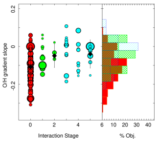
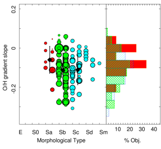
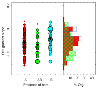
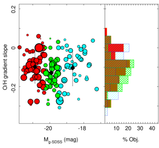
Figure 15: Top-left panel: Distribution of the slopes of the abundance gradients as a function of the interaction stage of the galaxies, when the galactocentric distances are normalized to the effective radius derived by a growth curve analysis. The colors of the symbols and the corresponding histograms indicate three types of galaxies based on the interaction: (i) no signatures of interaction (red), (ii) galaxies with close companions and/or in an early interaction stage (green), and (iii) galaxies under clear collision or evolved mergers (blue). Top-right panel: Similar distribution of slopes as a function of the morphological classification of the galaxies. The colors of the symbols and the corresponding histograms indicate three types of galaxies based on their morphology: (i) Early spirals, SO-Sa (red), (ii) intermediate spirals, Sab-Sb (green) and (iii) Late spirals, Sc-Sm (blue). Bottom-left panel: Similar distribution of slopes as a function of the presence or absence of bars. The colors of the symbols and the corresponding histograms indicate three types of galaxies: (i) clearly non-barred (red), (ii) not clear if there is a bar or not (green) and (iii) clearly barred galaxies (blue). Bottom-right panel: Similar distribution of slopes as a function of the absolute magnitude of the galaxies. The colors of the symbols and the corresponding histograms indicate three types of galaxies based on the luminosity: (i) luminous galaxies, $M_{g-SDSS}<-20.25$ mag (red), (ii) intermediate galaxies $-19.5<M_{g-SDSS}<-20.25$ mag (green) and (iii) faint galaxies $M_{g-SDSS}>-19.5$ mag (blue). The size of the symbols are inversely proportional to the derived error in the slope for all the panels.

To derive the disk effective radius it is required to fit that the outer portion of the SBP clearly dominated by an exponential disk. As is illustrated in the right panels of Fig. 13, in some cases there is almost no deviation from an exponential disk over the full spatial range covered by the SBP (e.g., UGC00312). However, in other cases there is a clear deviation in the inner regions due to the presence of a bulge (e.g., NGC7716). To minimize the effect of the bulge in this derivation we perform an iterative procedure, in which the SBP, represented in surface brightness magnitudes, was fitted with a linear regression. In each stage of the iteration the brightest value of the SBP was removed, and the regression was repeated. The iteration stops when only half of the original values remains in the SBP. From the set of regressions it was adopted that one with the highest correlation coefficient between the semi-major axis and the surface brightness magnitude.

The procedure was tested visually, as illustrated in Fig. 13, showing that it provides a good fit for the linear regime (i.e., the disk-dominated regime), excluding in most of the cases the central regions dominated by a bulge. Obviously, the procedure works better for those galaxies that are still dominated by disk in most of the SBP, and provides the worst results for those ones dominated by a bulge. However, this would be a general limitation to any other proposed method with the same aim.

Figure 14, right panel, shows the comparison between the effective radius derived using the growth-curve method and the the disk effective radius extracted from the iterative fit of the SBP. The size and color of the symbols represent the same morphological segregation shown in the left panel. As expected the late-type galaxies, disk-dominated, are clustered closer to the one-to-one relation, while most of the earlier-type ones, with brighter bulges, are shifted towards larger disk effective radius.

Appendix B Dependence of the results on the derivation of the disk effective radius

The main result described along the current study is that all undisturbed galaxies with a disk present a similar radial abundance gradient, with a characteristic slope, when the galactocentric distances are normalized to the disk effective radius. This characteristic slope seems to be independent of other properties of the galaxies, like morphological types, presence of a bars and absolute magnitudes or stellar masses. However, this result relies on the definition of the disk effective radius and its derivation, based on the surface brightness profile analysis described in the previous section.

The disk effective radius is a non-standard scale-length, that we have introduced to characterize the size of the disk in galaxies with different morphologies. Therefore, it is important to illustrate how our results are affected by this adopted normalization of the radial distances. To do so we repeat the analysis using the standard effective radius derived using the growth-curve analysis ($r_{e,GC}$), to normalize the abundance gradients, instead of the disk effective radius. As we already indicated the growth curve effective radius has been derived independently using to different procedures providing reliable and consistent results (Fig. 14, left panel).

Figure 15 shows the distribution of the new slopes obtained when normalizing to these effective radius, along the same structural parameters of the galaxies shown in Fig. 8. Despite the fact that individual slopes change, in particular for the galaxies of earlier type, all the results described in Section 4.2 remain valid:

• Galaxies with evidence of interaction or in a clear merging process present an oxygen abundance gradient flatter than those without any clear evidence of interaction. The difference is statistically significant, both using KS- or a $t$-test for the different distributions. The characteristic slope for non-interacting galaxies it is not affected by the selection of the normalization radius, with a mean value of $\alpha_{O/H}=-$0.11$\pm$0.09 dex/$r_{e}$ (although the dispersion suffer a slightly increase).

• The average slope for earlier type galaxies is slightly flatter when normalizing by $r_{e,GC}$, instead of the disk $r_{e}$: $\alpha_{O/H,Sa/S0}=-$0.06$\pm$0.08 dex/$r_{e,GC}$ instead of $\alpha_{O/H,Sa/S0}=-$0.08$\pm$0.08 dex/$r_{e}$. However, there is no significant different in the distribution of slopes, either using a KS- or a $t$-test analysis.

• Neither the average slopes nor the distribution of slopes change significantly depending on the presence or absence of a bar in the galaxies. The use of the total or disk effective radius seems to be irrelevant for the comparison of abundance gradients for barred an unbarred galaxies.

• The abundance gradient slopes normalized by $r_{e,GC}$ do not present any dependence in the absolute magnitudes, the stellar masses or the concentration indices of the galaxies.

In summary, although the slopes of the individual gradients for each galaxy change when normalizing by the disk $r_{e}$ or the $r_{e,GC}$, in general the statistical results are basically the same. The main effect, as expected, is found in the slope of the earlier type galaxies (Sa/S0), that present slightly flatter gradients. This is expected, since for these galaxies the disk $r_{e}$ is larger than the growth curve one, due to the presence of a bulge. For those galaxies the derivation of the disk $r_{e}$ is also more complicated, for the same reason. However, the fact that the slope of the abundance gradient becomes more similar for these galaxies to the one derived for the latter type ones, when using the disk effective radius, indicate that (i) the use of this radius provides a better characterization for the gradient and (ii) the metal enrichment seems to be clearly dominated by the growth of the disk, rather than other non-secular processes.