Estimation of the characteristic exponent of stable laws

Abstract

A statistical algorithm for estimating the characteristic parameter $\alpha$ of the stable law is presented and the estimate of its quadratic deviation is obtained in the paper. This algorithm is applied in the description of the fluctuation induced flux in the edge region of the plasma cord.

1 Introduction

The importance of investigating stable laws stems from the fact that all kinds of limit distributions of linearly-normed sums of an infinitely increasing number of independent identically distributed random variable are stable laws. This fact stipulates the application of stable laws in the problems of economics, physics, and other spheres of science. The latter makes the problem of estimating the parameters of stable laws very important.

In the book of Zolotarev (1986) the major features of the stable law are described. A class of stable distributions comprises a four parametric family of the functions $g(x;\alpha,\beta,\gamma,\lambda)$ with the parameters

$$0<\alpha\leqslant 2,\quad-1\leqslant\beta\leqslant 1,\quad-\infty<\gamma<\infty,\quad\lambda>0$$

(we shall call the parameter values admissible). This class of distributions is usually defined by the corresponding set of characteristic functions that can be written, e.g. in the following way (see Zolotarev (1986))

$$\hat{g}(k;\alpha,\beta,\lambda,\gamma)=\left\{\begin{array}[]{ll}\exp\left\{\lambda\left(ik\gamma-|k|^{\alpha}+i|k|^{\alpha}\beta\tan\left(\frac{\pi}{2}\alpha\right)\mathrm{sign}k\right)\right\},&\alpha\neq 1\\ \exp\left\{\lambda\left(ik\gamma-|k|^{\alpha}-ik\beta\frac{2}{\pi}\log|k|\right)\right\},&\alpha=1\end{array}\right.,$$

The class of stable distributions includes the normal distribution $(\alpha=2)$, Cauchy distribution $(\alpha=1)$ and the Levy distribution $(\alpha=1/2)$ together with that symmetric to it ($\alpha=1/2,\beta=-1$). Naturally, those variants of stable laws that appear due to a change in the values of unfixed parameters $\gamma$ and $\lambda$ should also be attributed to them. In other cases we did not succeed in expressing the density of stable distributions by elementary functions.

The problem of parameter estimation of stable laws is hampered by the absence of explicit expressions of densities. However, there are already a lot of works devoted to this problem. In our work the exponent $\alpha$ of stable laws is estimated. The estimation is based on the method, proposed by V. Zolotarev, for evaluating the parameters $\gamma,\theta,\tau$ of strictly stable random variables. The estimation of quadratic deviation of the constructed estimate has been obtained.

Before stating the main problem of this work we recall some results obtained in the book of Zolotarev (1986). Let there be a sample $X_{1},X_{2},\dots,X_{n}$ of independent identically distributed random variables (i.i.d.r.v.) having a strictly stable distribution with the characteristic function

$$\hat{g}(k;\nu,\theta,\tau)=\exp\left\{-\exp\left\{\nu^{-1/2}\left(\log|k|+\tau-i\frac{\pi}{2}\theta\mathrm{sign}k\right)+\bbbc\left(\nu^{-1/2}-1\right)\right\}\right\},$$ (1)

where $\bbbc=0.577\dots$ is the Euler constant and the parameters are varying within the limits of the interval $\nu\geqslant 1/4$, $|\theta|\leqslant\min(1,2\sqrt{\nu}-1)$, $\tau<\infty$. According to this sample we construct two sets of independent identically distributed (within the framework of each sample) random variables $U_{i}=\mathrm{sign}Y_{i}$ and $V_{i}=\log|Y_{i}|$, $i=1,\dots,n$. Then the estimator

$$\tilde{\theta}=A_{U},\quad\tilde{\tau}=A_{V},\quad$$ (2)

$$\tilde{\nu}=\max\left(\hat{\nu},\left(1+|\tilde{\theta}|\right)^{2}/4\right)$$ (3)

will be statistical estimates $\tilde{\nu},\tilde{\theta}$ and $\tilde{\tau}$ of the parameters $\nu,\theta,$ and $\tau$, where

$$\hat{\nu}=\frac{6}{\pi^{2}}B^{2}_{V}-\frac{3}{2}B^{2}_{U}+1,$$ (4)

and

$$A_{X}=\frac{1}{n}\sum_{j=1}^{n}X_{j},\quad B_{X}^{2}=\frac{1}{n-1}\sum_{j=1}^{n}\left(X_{j}-A_{X}\right)^{2}$$

are the sample mean and variance.

The basic results of this work are as follows:

Theorem 1.1.

The estimate $\tilde{\alpha}=1/\sqrt{\tilde{\nu}}$ of the parameter $\alpha$ is asymptotically unbiased of order $1/\sqrt{n}$ and its quadratic deviation satisfies the inequality

$$\mathsf{E}\left(\hat{\alpha}-\alpha\right)^{2} \leqslant\frac{\mathsf{E}(\hat{\nu}-\nu)^{2}}{4\nu^{3}}+\frac{12}{n\nu^{3/2}}\sqrt{\mathsf{E}(\hat{\nu}-\nu)^{2}}\left(P_{3}^{2}+\frac{\sqrt{P_{3}^{\prime}}}{n^{1/8}}\right)$$

$$+144\left(P_{3}^{4}/n^{2}+P_{3}^{\prime}/n^{9/4}\right),$$ (5)

where the expressions $P_{3}$, $P_{3}^{\prime}$ will be defined later.

The results obtained considerably improved the estimate of quadratic deviation of the parameter $\alpha$ obtained in Yanushkevichiene (1981). In addition, an experimental research has been performed here.

2 Algorithm for estimating the parameters of strictly stable laws

Proposition 2.1.

Transformation (3) can only decrease the quadratic deviation of the estimate from the real value of the parameter.

Proof.

If $\hat{\nu}\geqslant(1+|\tilde{\theta}|)^{2}/4$, then $\tilde{\nu}=\hat{\nu}$ and the proposition is obvious. If $\hat{\nu}<(1+|\tilde{\theta}|)^{2}/4$, then $\tilde{\nu}=(1+|\tilde{\theta}|)^{2}/4$. Taking into consideration that, for a given value $\theta$, the domain of values of the parameter $\nu$ is defined from the condition $\nu\geqslant(1+|\theta|)^{2}/4$, we obtain the inequality

$$|\tilde{\nu}-\nu|<|\hat{\nu}-\nu|,$$

which finally proves the proposition. ∎

Next, let there be a sequence $Y_{1},Y_{2},\dots,Y_{n}$ of i.i.d.r.v’s having the stable distribution with the characteristic function

$$\hat{g}(k;\alpha,\beta,\lambda,\gamma)=\left\{\begin{array}[]{ll}\exp\left\{\lambda\left(ik\gamma-|k|^{\alpha}+i|k|^{\alpha}\beta\tan\left(\frac{\pi}{2}\alpha\right)\mathrm{sign}k\right)\right\},&\alpha\neq 1\\ \exp\left\{\lambda\left(ik\gamma-|k|^{\alpha}-ik\beta\frac{2}{\pi}\log|k|\right)\right\},&\alpha=1\end{array}\right.,$$

where the parameters are varying within scope $0<\alpha\leqslant 2$, $-1\leqslant\beta\leqslant 1$, $-\infty<\gamma<\infty$, $\lambda>0$. The parameters $\nu,\theta,\tau$ are connected with the parameter $\alpha,\beta,\lambda,\gamma$ by the expressions

$$\nu = \alpha^{-2},$$

$$\theta = \left\{\begin{array}[]{ll}\displaystyle\frac{2}{\pi\alpha}\arctan\left(\beta\tan\left(\frac{\pi\alpha}{2}\right)\right),&\nu\neq 1,\\[14.22636pt] \displaystyle\frac{2}{\pi}\arctan(\gamma),&\nu=1,\end{array}\right.$$ (8)

$$\tau = \left\{\begin{array}[]{ll}\displaystyle(1/\alpha)\left[\log\lambda-\log\left(\cos\left(\arctan\left(\beta\tan(\pi\alpha/2)\right)\right)\right)-\bbbc(\alpha-1)\right],&\nu\neq 1,\\ \log\lambda-\log\left(\cos(\arctan\gamma)\right),&\nu=1.\end{array}\right.$$ (11)

Construction of the estimates $\tilde{\alpha},\tilde{\beta},\tilde{\lambda},\tilde{\gamma}$ of the parameters $\alpha,\beta,\lambda,\gamma$ is based on the application of estimates (2) and (3). To this end, the initial sequence $Y_{1},Y_{2},\dots,Y_{n}$ should be transformed so that the random variables, included in the new sample $Y_{1}^{\prime},Y_{2}^{\prime},\dots,Y_{m}^{\prime}$, belonged to the class of strictly stable laws. In the book of Zolotarev (1986), the transformation

$$Y_{j}^{\prime}=Y_{3j-2}-1/2(Y_{3j-1}+Y_{2j}),\quad j=1,2,\dots,3n.$$ (12)

is selected as this kind of transformation. As a result of the transformation, the random variables $Y^{\prime}_{j}$ have the distribution $g(x;\alpha,\beta^{\prime},\lambda^{\prime},\gamma^{\prime})$, where the parameters $\beta^{\prime},\lambda^{\prime},\gamma^{\prime}$ are connected with that of the distribution of the initial sample through the relations

$$\beta^{\prime} = \frac{1-2^{1-\alpha}}{1+2^{1-\alpha}}\beta,$$

$$\lambda^{\prime} = \left(1+2^{1-\alpha}\right)\lambda,$$

$$\gamma^{\prime} = \left\{\begin{array}[]{cl}0,&\mbox{ }\alpha\neq 1,\\ -\frac{\log 2}{\pi}\beta,&\mbox{ }\alpha=1,\end{array}\right.$$ (15)

and the characteristic exponent of the stable law does not change. Hence we can see that, if $\alpha\neq 1$, then $\gamma=0$, and if $\alpha=1$, then $\beta=0$. It means that the random variable $Y^{\prime}$ belongs to the class of strictly stable laws and its characteristic function can be represented in the form (1). This fact allows us to apply algorithm (2) to the sample $Y_{j}^{\prime}$ and to obtain estimates $\tilde{\nu}^{\prime},\tilde{\theta}^{\prime},\tilde{\tau}^{\prime}$. It ought to be noted here that application of transformation (12) leads to contraction of the domain of change of the parameters $\theta^{\prime},\tau^{\prime}$. In order to estimate the parameters of the stable law, we choose the following expressions

$$\tilde{\nu}^{*}=\tilde{\nu}^{\prime},\quad\tilde{\theta}^{*}=\min(H(\tilde{\nu}^{\prime}),|\tilde{\theta}^{\prime}|)\mathrm{sign}\tilde{\theta}^{\prime},\quad\tilde{\tau}^{*}=\tilde{\tau}^{\prime},$$ (16)

where the estimates $\tilde{\nu}^{\prime},\tilde{\theta}^{\prime},\tilde{\tau}^{\prime}$ are obtained by the sequence $Y_{1}^{\prime},\dots,Y_{m}^{\prime}$ with the aid of formulas (2) and (3), and

$$H(t)=\left\{\begin{array}[]{ll}\frac{2}{\pi}\sqrt{t}\arctan\left(\frac{1-\exp\left\{(1-1/\sqrt{t})\log 2\right\}}{1+\exp\left\{(1-1/\sqrt{t})\log 2\right\}}\tan\left(\frac{\pi}{2\sqrt{t}}\right)\right),&t\neq 1\\ \frac{2}{\pi}\arctan\left(\frac{\log 2}{\pi}\right),&t=1.\end{array}\right.$$

Proposition 2.2.

Transformation of the parameters $\theta$ in (16) can only diminish the value of mean-square deviation of the estimate $\tilde{\theta}^{*}$.

The proof is analogous to that of Proposition 2.1.

We obtain the following expressions

$$\tilde{\alpha} = 1/\sqrt{\tilde{\nu}^{*}}$$ (17)

$$\tilde{\beta} = \left\{\begin{array}[]{cl}\displaystyle\left(\frac{1+2^{1-\tilde{\alpha}}}{1-2^{1-\tilde{\alpha}}}\right)\frac{\tan\left(\frac{\pi}{2}\tilde{\theta}^{*}\tilde{\alpha}\right)}{\tan\left(\frac{\pi}{2}\tilde{\alpha}\right)},&\tilde{\alpha}\neq 1\\ \displaystyle-\frac{\pi}{\log 2}\tan\left(\frac{\pi}{2}\tilde{\theta}^{*}\right),&\tilde{\alpha}=1\end{array}\right.$$ (20)

$$\tilde{\lambda} = \left\{\begin{array}[]{cl}\displaystyle\frac{\cos\left(\frac{\pi}{2}\tilde{\theta}^{*}\tilde{\alpha}\right)}{1+2^{1-\tilde{\alpha}}}\exp\left\{\tilde{\tau}^{*}\tilde{\alpha}+\bbbc\left(\tilde{\alpha}-1\right)\right\},&\tilde{\alpha}\neq 1\\ \displaystyle(1/2)\exp\{\tilde{\tau}^{*}\}\cos\left(\pi\tilde{\theta}^{*}/2\right),&\tilde{\alpha}=1\end{array}\right.$$ (23)

for the estimates $\tilde{\alpha},\tilde{\beta},\tilde{\lambda}$.

3 Evaluation of mean-square deviation of the estimate $\tilde{\alpha}$

We will focus our attention on obtaining the estimate of mean-square deviation of $\tilde{\alpha}$. The idea of finding the estimate consist in the expansion of expression (17) in a Taylor series with respect to the parameter $\tilde{\nu}$ in the neighborhood of the true value $\nu$. However, before stating a theorem for estimating the mean-square deviation, we shall prove a number of lemmas.

Lemma 3.1.

Let $X$ be a strictly stable random variable. Then the following expressions hold.

$$\mathsf{E}\log|X| = \tau,\qquad\mathsf{E}\log^{2}|X|=\tau^{2}+\mathsf{D}V,$$

$$\mathsf{E}\log^{3}|X| = \tau^{3}+3\tau\mathsf{D}V+2\zeta(3)\left(\nu^{3/2}-1\right),$$

$$\mathsf{E}\log^{4}|X| = \tau^{4}+6\tau^{2}\mathsf{D}V+8\tau\zeta(3)\left(\nu^{3/2}-1\right)+3(\mathsf{D}V)^{2}$$

$$+ \pi^{4}\left(\left(1-\theta^{4}\right)/8+\left(\nu^{2}-1\right)/15\right),$$

$$\mathsf{E}\log^{5}|X| = \tau^{5}+10\tau^{3}\mathsf{D}V+20\tau^{2}\zeta(3)\left(\nu^{3/2}-1\right)+15\tau(\mathsf{D}V)^{2}$$

$$+ 5\tau\pi^{4}\left(\frac{1-\theta^{4}}{8}+\frac{\nu^{2}-1}{15}\right)+20\zeta(3)\left(\nu^{3/2}-1\right)\mathsf{D}V$$

$$+ 24\zeta(5)\left(\nu^{5/2}-1\right),$$

$$\mathsf{E}\log^{6}|X| = \tau^{6}+15\tau^{4}\mathsf{D}V+40\tau^{3}\zeta(3)\left(\nu^{3/2}-1\right)+45\tau^{2}(\mathsf{D}V)^{2}+15(\mathsf{D}V)^{3}$$

$$+ 15\tau^{2}\pi^{4}\left(\frac{1-\theta^{4}}{8}+\frac{\nu^{2}-1}{15}\right)+120\tau\zeta(3)\left(\nu^{3/2}-1\right)\mathsf{D}V$$

$$+ 40\zeta^{2}(3)\left(\nu^{3/2}-1\right)^{2}+144\tau\zeta(5)\left(\nu^{5/2}-1\right)$$

$$+ 15\pi^{4}\left(\frac{1-\theta^{4}}{8}+\frac{\nu^{2}-1}{15}\right)\mathsf{D}V+8\pi^{6}\left(\frac{1-\theta^{6}}{32}+\frac{\nu^{3}-1}{63}\right),$$

$$\mathsf{E}\log^{7}|X| = \tau^{7}\!+\!21\tau^{5}\mathsf{D}V\!+\!70\tau^{4}\zeta(3)\left(\nu^{3/2}-1\right)\!+\!35\tau^{3}\pi^{4}\left(\frac{1-\theta^{4}}{8}+\frac{\nu^{2}-1}{15}\right)$$

$$+ 105\tau(\mathsf{D}V)^{3}+420\tau^{2}\zeta(3)\left(\nu^{3/2}-1\right)\mathsf{D}V+504\tau^{2}\zeta(5)\left(\nu^{5/2}-1\right)$$

$$+ 210\zeta(3)\left(\nu^{3/2}-1\right)(\mathsf{D}V)^{2}+105\tau\pi^{4}\left(\frac{1-\theta^{4}}{8}+\frac{\nu^{2}-1}{15}\right)\mathsf{D}V$$

$$+ 56\tau\pi^{6}\left(\frac{1-\theta^{6}}{32}+\frac{\nu^{3}-1}{63}\right)+504\zeta(5)\left(\nu^{5/2}-1\right)\mathsf{D}V$$

$$+ 70\zeta(3)\left(\nu^{3/2}\!-\!1\right)\pi^{4}\!\left(\frac{1-\theta^{4}}{8}+\frac{\nu^{2}-1}{15}\right)+280\tau\zeta^{2}(3)\left(\nu^{3/2}-1\right)^{2}$$

$$+ 720\zeta(7)\left(\nu^{7/2}-1\right)+105\tau^{3}(\mathsf{D}V)^{2}$$

$$\mathsf{E}\log^{8}|X| = \tau^{8}+28\tau^{6}\mathsf{D}V+112\tau^{5}\zeta(3)\left(\nu^{3/2}-1\right)+210\tau^{4}(\mathsf{D}V)^{2}$$

$$+ 70\tau^{4}\pi^{4}\left(\frac{1-\theta^{4}}{8}+\frac{\nu^{2}-1}{15}\right)+420\tau^{2}(\mathsf{D}V)^{3}$$

$$+ 1120\tau^{3}\zeta(3)\left(\nu^{3/2}-1\right)\mathsf{D}V+105(\mathsf{D}V)^{4}+1344\tau^{3}\zeta(5)\left(\nu^{5/2}-1\right)$$

$$+ 420\tau^{2}\pi^{4}\left(\frac{1-\theta^{4}}{8}+\frac{\nu^{2}-1}{15}\right)\mathsf{D}V+1680\tau(\mathsf{D}V)^{2}\zeta(3)\left(\nu^{3/2}-1\right)$$

$$+ 224\tau^{2}\pi^{6}\left(\frac{1-\theta^{6}}{32}+\frac{\nu^{3}-1}{63}\right)+1120\tau^{2}\zeta^{2}(3)\left(\nu^{3/2}-1\right)^{2}$$

$$+ 210(\mathsf{D}V)^{2}\pi^{4}\left(\frac{1-\theta^{4}}{8}+\frac{\nu^{2}-1}{15}\right)$$

$$+ 560\tau\zeta(3)\left(\nu^{3/2}-1\right)\pi^{4}\left(\frac{1-\theta^{4}}{8}+\frac{\nu^{2}-1}{15}\right)$$

$$+ 1120\zeta^{2}(3)\left(\nu^{3/2}-1\right)^{2}\mathsf{D}V+4032\tau\zeta(5)\left(\nu^{5/2}-1\right)\mathsf{D}V$$

$$+ 35\pi^{8}\left(\frac{1-\theta^{4}}{8}+\frac{\nu^{2}-1}{15}\right)^{2}+5760\tau\zeta(7)\left(\nu^{7/2}-1\right)$$

$$+ 224\pi^{6}\left(\frac{1-\theta^{6}}{32}+\frac{\nu^{3}-1}{63}\right)\mathsf{D}V$$

$$+ 2688\zeta(3)\left(\nu^{3/2}-1\right)\zeta(5)\left(\nu^{5/2}-1\right)$$

$$+ 16\pi^{8}\left(\frac{17(1-\theta^{8})}{256}+\frac{\nu^{4}-1}{30}\right),$$

Here $\mathsf{D}V=\frac{\pi^{2}}{4}\left(1-\theta^{2}\right)+\frac{\pi^{2}}{6}(\nu-1)$ and $\zeta(x)$ is the zeta function.

Proof.

It follows from the Theorem 3.6.1 of Zolotarev (1986). ∎

Let us introduce the notations $\bar{U}=U-\mathsf{E}U$, $\bar{V}=V-\mathsf{E}V$. Applying expression (2), it is easy to show that

$$\mathsf{E}U=\theta,\quad\mathsf{E}V=\tau.$$

The following lemma is valid.

Lemma 3.2.

For centered moments of the random variable $U$ the equalities

$$\begin{split}\mathsf{E}\bar{U}&=0,\quad\mathsf{E}\bar{U}^{2}=1-\theta^{2},\\ \mathsf{E}\bar{U}^{3}&=2\theta(\theta^{2}-1),\quad\mathsf{E}\bar{U}^{4}=1+2\theta^{2}-3\theta^{4},\\ \mathsf{E}\bar{U}^{5}&=4\theta(\theta^{4}-1),\quad\mathsf{E}\bar{U}^{6}=1+9\theta^{2}-5\theta^{4}-5\theta^{6},\\ \mathsf{E}\bar{U}^{7}&=2\theta(3\theta^{6}+7\theta^{4}-7\theta^{2}-3),\\ \mathsf{E}\bar{U}^{8}&=1+20\theta^{2}+14\theta^{4}-28\theta^{6}-7\theta^{8},\end{split}$$ (24)

hold.

Proof.

Consider, for example, the fifth central moment. Taking into consideration that

$$\mathrm{sign}^{n}U=\left\{\begin{array}[]{ll}\mathrm{sign}U,&\mbox{if}\ n\ \mbox{is odd}\\ 1,&\mbox{if}\ n\ \mbox{is even},\end{array}\right.,$$

we get

$$\mathsf{E}(U - \theta)^{5}=\mathsf{E}\left[\mathrm{sign}^{5}U-5\theta\mathrm{sign}^{4}U+10\theta^{2}\mathrm{sign}^{3}U-10\theta^{3}\mathrm{sign}^{2}U\right.$$

$$+ \left.5\theta^{4}\mathrm{sign}U-\theta^{5}\right]=\theta-5\theta+10\theta^{3}-10\theta^{3}+5\theta^{5}-\theta^{5}=4\theta(\theta^{4}-1).$$

The remaining equalities are proved by analogously. ∎

Lemma 3.3.

The expressions

$$\begin{split}\mathsf{E}\bar{V}&=0,\quad\mathsf{E}\bar{V}^{2}=\frac{\pi^{2}}{4}\left(1-\theta^{4}\right)+\frac{\pi^{2}}{6}\left(\nu-1\right)=\mathsf{D}V,\\ \mathsf{E}\bar{V}^{3}&=2\zeta(3)\left(\nu^{3/2}-1\right),\quad\mathsf{E}\bar{V}^{4}=\pi^{4}\left(\frac{1-\theta^{4}}{8}+\frac{\nu^{2}-1}{15}\right)+3(\mathsf{D}V)^{2},\\ \mathsf{E}\bar{V}^{5}&=20\zeta(3)\left(\nu^{3/2}-1\right)\mathsf{D}V+24\zeta(5)\left(\nu^{5/2}-1\right),\\ \mathsf{E}\bar{V}^{6}&=15(\mathsf{D}V)^{3}+15\pi^{4}\left(\frac{1-\theta^{4}}{8}+\frac{\nu^{2}-1}{15}\right)\mathsf{D}V+8\pi^{6}\left(\frac{1-\theta^{6}}{32}+\frac{\nu^{2}-1}{63}\right)\\ &+40\zeta^{2}(3)\left(\nu^{3/2}-1\right)^{2},\\ \mathsf{E}\bar{V}^{7}&=105(\mathsf{D}V)^{4}+210(\mathsf{D}V)^{2}\pi^{4}\left(\frac{1-\theta^{4}}{8}+\frac{\nu^{2}-1}{15}\right)\\ &+2688\zeta(3)\left(\nu^{3/2}-1\right)\zeta(5)\left(\nu^{5/2}-1\right)\\ &+8\pi^{8}\left(\frac{17(1-\theta^{8})}{128}+\frac{\nu^{4}-1}{15}\right).\end{split}$$ (25)

are valid for the central moments of the random variable $V$

Proof.

Let us consider, for instance, the fifth central moment. Making use of the results of Lemma 3.1 we get

$$\mathsf{E}\bar{V}^{5} = \mathsf{E}\left(V-\mathsf{E}V\right)^{5}=\mathsf{E}V^{5}-5\mathsf{E}V^{4}\tau+10\mathsf{E}V^{3}\tau^{2}-10\mathsf{E}V^{2}\tau^{3}+5\mathsf{E}V\tau^{4}-\tau^{5}$$

$$= \tau^{5}\!+\!10\tau^{3}\mathsf{D}V\!+\!20\tau^{2}\zeta(3)\left(\nu^{3/2}\!-\!1\right)\!+\!15\tau(\mathsf{D}V)^{2}$$

$$+ 5\tau\pi^{4}\left(\frac{1-\theta^{4}}{8}+\frac{\nu^{2}-1}{15}\right)+20\zeta(3)\left(\nu^{3/2}-1\right)\mathsf{D}V$$

$$+ 24\zeta(5)\left(\nu^{5/2}-1\right)\!-\!5\tau^{5}\!-\!30\tau^{3}\mathsf{D}V-40\tau^{2}\zeta(3)\left(\nu^{3/2}-1\right)-15\tau(\mathsf{D}V)^{2}$$

$$- 5\tau\pi^{4}\left(\frac{1-\theta^{4}}{8}+\frac{\nu^{2}-1}{15}\right)+10\tau^{5}+30\tau^{3}\mathsf{D}V+20\tau^{2}\zeta(3)\left(\nu^{3/2}-1\right)$$

$$- 10\tau^{5}-10\tau^{3}\mathsf{D}V+5\tau^{5}-\tau^{5}$$

$$= 20\zeta(3)\left(\nu^{3/2}-1\right)\mathsf{D}V+24\zeta(5)\left(\nu^{5/2}-1\right).$$

All the remaining equalities are obtained similarly. ∎

Let us introduce the notations:

$$P_{1} = 16\left(15\theta^{2}-71\theta^{4}+26\theta^{6}-45\theta^{8}\right)+\frac{12}{n-1}\left(5-96\theta^{2}+302\theta^{4}-356\theta^{6}\right.$$

$$+ \left.155\theta^{8}\right)=\frac{4}{(n-1)^{2}}\left(5-52\theta^{2}+134\theta^{4}+132\theta^{6}+45\theta^{8}\right).$$

$$P_{2} = 4\left\{18(\mathsf{D}V)^{4}\!+\!39(\mathsf{D}V)^{2}\pi^{4}\left(\frac{1-\theta^{4}}{8}\!+\!\frac{\nu^{2}-1}{15}\right)\!+\!96\zeta^{2}(3)\left(\nu^{3/2}-1\right)^{2}\!\mathsf{D}V\right.$$

$$+ 8\pi^{8}\left(\frac{1-\theta^{4}}{8}+\frac{\nu^{2}-1}{15}\right)^{2}+48\pi^{6}\left(\frac{1-\theta^{6}}{32}+\frac{\nu^{3}-1}{63}\right)\mathsf{D}V$$

$$+ \left.384\zeta(3)\left(\nu^{3/2}-1\right)\zeta(5)\left(\nu^{5/2}-1\right)+2\pi^{8}\left(\frac{17(1-\theta^{6})}{128}+\frac{\nu^{4}-1}{15}\right)\right\}$$

$$+ \frac{12}{n-1}\left\{15(\mathsf{D}V)^{4}+25(\mathsf{D}V)^{2}\pi^{4}\left(\frac{1-\theta^{4}}{8}+\frac{\nu^{2}-1}{15}\right)\right.$$

$$+ 16\pi^{6}\left(\frac{1-\theta^{6}}{32}+\frac{\nu^{3}-1}{63}\right)\mathsf{D}V+32\zeta^{2}(3)\left(\nu^{3/2}-1\right)^{2}\mathsf{D}V$$

$$+ \left.2\pi^{8}\left(\frac{1-\theta^{4}}{8}+\frac{\nu^{2}-1}{15}\right)^{2}\right\}+\frac{12}{(n-1)^{2}}\left\{-32\zeta^{2}(3)\left(\nu^{3/2}-1\right)^{2}\mathsf{D}V\right.$$

$$- 128\zeta(3)\left(\nu^{3/2}-1\right)\zeta(5)\left(\nu^{5/2}-1\right)+12(\mathsf{D}V)^{2}\pi^{4}\left(\frac{1-\theta^{4}}{8}+\frac{\nu^{2}-1}{15}\right)$$

$$+ \left.13(\mathsf{D}V)^{4}\right\}+\frac{8}{(n-1)^{3}}\left\{\pi^{8}\left(\frac{1-\theta^{4}}{8}+\frac{\nu^{2}-1}{15}\right)^{2}+6(\mathsf{D}V)^{4}\right.$$

$$- \left.48\zeta^{2}(3)\left(\nu^{3/2}-1\right)^{2}\mathsf{D}V\right\},$$

$$P_{3} = 3\sqrt[4]{3}\sqrt{\theta^{2}(1-\theta^{2})}+\frac{6\sqrt[4]{3}}{\pi^{2}}\sqrt{\pi^{4}\left(\frac{1-\theta^{4}}{8}+\frac{\nu^{2}-1}{15}\right)+3(\mathsf{D}V)^{2}},$$ (26)

$$P_{3}^{\prime} = n^{1/4}\left(P_{3}+\frac{3}{2}\left(\frac{|P_{1}|}{n}\right)^{1/4}+\frac{6}{\pi^{2}}\left(\frac{|P_{2}|}{n}\right)^{1/4}\right)^{4}-n^{1/4}P_{3}^{4}.$$ (27)

Lemma 3.4.

The inequality

$$\mathsf{E}\left(\tilde{\nu}-\nu\right)^{4}\leqslant\frac{P_{3}^{4}}{n^{2}}+\frac{P_{3}^{\prime}}{n^{9/4}}$$ (28)

is true.

Proof.

By combining (4) and assumption 2.1, we get

$$\begin{split}\mathsf{E}\left(\tilde{\nu}\right.&-\left.\nu\right)^{4}\leqslant\mathsf{E}\left(\hat{\nu}-\nu\right)^{4}=\mathsf{E}\left(\frac{6}{\pi^{2}}S_{V}^{2}-\frac{3}{2}S_{U}^{2}+1-\mathsf{E}\left(\frac{6}{\pi^{2}}S_{V}^{2}-\frac{3}{2}S_{U}^{2}+1\right)\right)^{4}\\ &=\frac{6^{4}}{\pi^{8}}\mathsf{E}\left(B_{V}^{2}-\mathsf{E}B_{V}^{2}\right)^{4}-\frac{6^{4}}{\pi^{6}}\mathsf{E}\left\{\left(B_{V}^{2}-\mathsf{E}B_{V}^{2}\right)^{3}\left(B_{U}^{2}-\mathsf{E}B_{U}^{2}\right)\right\}\\ &+\frac{6\cdot 3^{4}}{\pi^{4}}\mathsf{E}\left\{\left(B_{V}^{2}-\mathsf{E}B_{V}^{2}\right)^{2}\left(B_{U}^{2}-\mathsf{E}B_{U}^{2}\right)^{2}\right\}\\ &-\frac{3^{4}}{\pi^{2}}\mathsf{E}\left\{\left(B_{V}^{2}-\mathsf{E}B_{V}^{2}\right)\left(B_{U}^{2}-\mathsf{E}B_{U}^{2}\right)^{3}\right\}\\ &+\frac{3^{4}}{2^{4}}\mathsf{E}\left(B_{U}^{2}-\mathsf{E}B_{U}^{2}\right)^{4}\leqslant\frac{6^{4}}{\pi^{8}}\mathsf{E}\left(B_{V}^{2}-\mathsf{E}B_{V}^{2}\right)^{4}\\ &-\frac{6^{4}}{\pi^{6}}\left(\mathsf{E}\left(B_{V}^{2}-\mathsf{E}B_{V}^{2}\right)^{4}\right)^{3/4}\left(\mathsf{E}\left(B_{U}^{2}-\mathsf{E}B_{U}^{2}\right)^{4}\right)^{1/4}\\ &+\frac{6\cdot 3^{4}}{\pi^{4}}\left(\mathsf{E}\left(B_{V}^{2}-\mathsf{E}B_{V}^{2}\right)^{4}\right)^{1/2}\left(\mathsf{E}\left(B_{U}^{2}-\mathsf{E}B_{U}^{2}\right)^{2}\right)^{1/2}\\ &-\frac{3^{4}}{\pi^{2}}\left(\mathsf{E}\left(B_{V}^{2}-\mathsf{E}B_{V}^{2}\right)^{4}\right)^{1/4}\left(\mathsf{E}\left(B_{U}^{2}-\mathsf{E}B_{U}^{2}\right)^{4}\right)^{3/4}+\frac{3^{4}}{2^{4}}\mathsf{E}\left(B_{U}^{2}-\mathsf{E}B_{U}^{2}\right)^{4}\\ &=\left(\frac{6}{\pi^{2}}\sqrt[4]{\mathsf{E}\left(B_{V}^{2}-\mathsf{E}B_{V}^{2}\right)^{4}}+\frac{3}{2}\sqrt[4]{\mathsf{E}\left(B_{U}^{2}-\mathsf{E}B_{U}^{2}\right)^{4}}\right)^{4}\end{split}$$ (29)

Thus we need to estimate the mathematical expectations $\mathsf{E}\left(B_{V}^{2}-\mathsf{E}B_{V}^{2}\right)^{4}$ and $\mathsf{E}\left(B_{U}^{2}-\mathsf{E}B_{U}^{2}\right)^{4}$.

Let $X_{i},\ i=1,2,\dots,n$ are the independent random variables with mathematical expectation $a$ and variance $b^{2}$. The equality

$$\mathsf{E}\left(B_{X}^{2}\right. -\left.\mathsf{E}B_{X}^{2}\right)^{4}=\mathsf{E}\left[\frac{n}{n-1}\left(\frac{1}{n}\sum_{i=1}^{n}X_{i}^{2}-\left(\frac{1}{n}\sum_{i=1}^{n}X_{i}\right)^{2}\right)-b^{2}\right]^{4}$$

$$= \mathsf{E}\left[\frac{n}{n-1}\frac{1}{n^{2}}\left(\sum_{i=1}^{n}X_{i}^{2}(n-1)-\sum_{i\neq j}X_{i}X_{j}\right)-b^{2}\right]^{4}$$

$$= \mathsf{E}\left[\frac{1}{n(n-1)}\left(\sum_{i=1}^{n}(X_{i}-a)^{2}(n-1)-\sum_{i\neq j}(X_{i}-a)(X_{j}-a)\right)-b^{2}\right]^{4}.$$

holds.

Let $Z_{i}=X_{i}-a$, then $\mathsf{E}Z_{i}=0$, and $\mathsf{E}Z_{i}^{2}=b^{2}$. Consequently, we get

$$\mathsf{E}\left(B_{Z}^{2}-\mathsf{E}B_{Z}^{2}\right)^{4}=\mathsf{E}\left[\frac{1}{n}\sum_{i=1}^{n}\left(Z_{i}^{2}-b^{2}\right)-\frac{1}{n(n-1)}\sum_{i\neq j}Z_{i}Z_{j}\right]^{4}$$

$$=\frac{1}{n^{4}}\mathsf{E}\left[\sum_{i=1}^{n}\left(Z_{i}^{2}-b^{2}\right)\right]^{4}=\frac{4}{n^{4}(n-1)}\mathsf{E}\left[\left(\sum_{i=1}^{n}\left(Z_{i}^{2}-b^{2}\right)\right)^{3}\sum_{i\neq j}Z_{i}Z_{j}\right]$$

$$+\frac{6}{n^{4}(n-1)^{2}}\mathsf{E}\left[\left(\sum_{i=1}^{n}\left(Z_{i}^{2}-b^{2}\right)\right)^{2}\left(\sum_{i\neq j}Z_{i}Z_{j}\right)^{2}\right]$$

$$-\frac{4}{n^{4}(n-1)^{3}}\mathsf{E}\left[\!\!\left(\sum_{i=1}^{n}\left(Z_{i}^{2}-b^{2}\right)\right)\!\!\!\left(\sum_{i\neq j}Z_{i}Z_{j}\right)^{3}\right]+\frac{1}{n^{4}(n-1)^{4}}\mathsf{E}\left[\sum_{i\neq j}Z_{i}Z_{j}\right]^{4}$$

$$=\frac{1}{n^{4}}n\mathsf{E}\left(Z_{i}^{2}-b^{2}\right)^{4}+\frac{3n(n-1)}{n^{4}}\left(\mathsf{E}\left(Z_{i}^{2}-b^{2}\right)^{2}\right)^{2}$$

$$-\frac{4}{n^{4}(n-1)}\mathsf{E}\left(\left(\sum_{i=1}^{n}\left(Z_{i}^{2}-b^{2}\right)^{3}+3\sum_{i\neq j}\left(Z_{i}^{2}-b^{2}\right)^{2}\left(Z_{j}^{2}-b^{2}\right)\right.\right.$$

$$+\left.\left.\sum_{i\neq j\neq k}\left(Z_{i}^{2}-b^{2}\right)\left(Z_{j}^{2}-b^{2}\right)\left(Z_{k}^{2}-b^{2}\right)\right)\sum_{i\neq j}Z_{i}Z_{j}\right)$$

$$+\frac{6}{n^{4}(n-1)^{2}}\mathsf{E}\left(\!\left(\sum_{i=1}^{n}\left(Z_{i}^{2}-b^{2}\right)^{2}\!+\sum_{i\neq j}\left(Z_{i}^{2}-b^{2}\right)\left(Z_{j}^{2}-b^{2}\right)\right)\!\left(2\sum_{i_{\neq}j}Z_{i}^{2}Z_{j}^{2}+\right.\right.$$

$$+\left.\left.4\sum_{i\neq j\neq k}Z_{i}^{2}Z_{j}Z_{k}+\sum_{i\neq j\neq k\neq m}Z_{i}Z_{j}Z_{k}Z_{m}\right)\right)$$

$$-\frac{4}{n^{4}(n-1)^{3}}\mathsf{E}\left(\sum_{i=1}^{n}\left(Z_{i}^{2}-b^{2}\right)\left(4\sum_{i\neq j}Z_{i}^{3}Z_{j}^{3}+\right.\right.24\sum_{i\neq j\neq k}Z_{i}^{3}Z_{j}^{2}Z_{k}$$

$$+8\sum_{i\neq j\neq k}Z_{i}^{2}Z_{j}^{2}Z_{k}^{2}+8\sum_{i\neq j\neq k\neq l}Z_{i}^{3}Z_{j}Z_{k}Z_{l}+30\sum_{i\neq j\neq k\neq l}Z_{i}^{2}Z_{j}^{2}Z_{k}Z_{l}$$

$$\left.\left.+12\sum_{i\neq j\neq k\neq l\neq m}Z_{i}^{2}Z_{j}Z_{k}Z_{l}Z_{m}+\sum_{i\neq j\neq k\neq l\neq m\neq p}Z_{i}Z_{j}Z_{k}Z_{l}Z_{m}Z_{p}\right)\right)$$

$$+\frac{1}{n^{4}(n-1)^{4}}\mathsf{E}\left(8\sum_{i\neq j}Z_{i}^{4}Z_{j}^{4}+48\sum_{i\neq j\neq k}Z_{i}^{4}Z_{j}^{2}Z_{k}^{2}+96\sum_{i\neq j\neq k}Z_{i}^{3}Z_{j}^{3}Z_{k}^{2}\right.$$

$$+\left.60\sum_{i\neq j\neq k\neq l}Z_{i}^{2}Z_{j}^{2}Z_{k}^{2}Z_{l}^{2}\right).$$

Taking into consideration that $\mathsf{E}Z=0$, we get $\mathsf{E}\sum_{i\neq j\neq k}Z_{i}^{a}Z_{j}^{b}Z_{k}=0$. It is easy to obtain, that

$$\mathsf{E}\left(B_{Z}^{2}-b^{2}\right)^{4}=\frac{1}{n^{3}}\left(\mathsf{E}Z^{8}-4\mathsf{E}Z^{6}b^{2}+6\mathsf{E}Z^{4}b^{4}-4\mathsf{E}Z^{2}b^{2}+b^{8}\right)$$

$$+\frac{3(n-1)}{n^{3}}\left(\mathsf{E}Z^{4}-b^{4}\right)^{2}-\frac{24}{n^{4}(n-1)}\mathsf{E}\left(\sum_{i\neq j}Z_{i}\left(Z_{i}^{2}-b^{2}\right)^{2}Z_{j}\left(Z_{j}^{2}-b^{2}\right)\right)$$

$$+\frac{6}{n^{4}(n-1)^{2}}\left(\left(\sum_{i}Z_{i}^{4}-2b^{2}\sum_{i}Z_{i}^{2}-nb^{4}\right)\right.\times$$

$$\times\left(2\sum_{i\neq j}Z_{i}^{2}Z_{j}^{2}+4\sum_{i\neq j\neq k}Z_{i}^{2}Z_{j}Z_{k}\right)+4\sum_{i\neq j}Z_{i}^{2}\left(Z_{i}^{2}-b^{2}\right)Z_{j}^{2}\left(Z_{j}^{2}-b^{2}\right)$$

$$+\left.8\sum_{i\neq j\neq k}Z_{i}^{2}Z_{j}\left(Z_{i}^{2}-b^{2}\right)\!\!\left(Z_{k}^{2}-b^{2}\right)Z_{k}\right)\!-\!\frac{4}{n^{4}(n-1)^{3}}\mathsf{E}\!\left(\!8\!\sum_{i\neq j}Z_{i}^{3}Z_{j}^{3}\left(Z_{i}^{2}-b^{2}\right)\right.$$

$$\left.+24\sum_{i\neq j\neq k}Z_{i}^{3}Z_{j}^{2}Z_{k}\left(Z_{k}^{2}-b^{2}\right)+24\sum_{i\neq j\neq k}Z_{i}^{2}Z_{j}^{2}Z_{k}^{2}\left(Z_{k}^{2}-b^{2}\right)\right)+\frac{8\left(\mathsf{E}Z^{4}\right)^{2}}{n^{3}(n-1)^{3}}$$

$$+\frac{48(n-2)\mathsf{E}Z^{4}b^{4}}{n^{3}(n-1)^{3}}+\frac{96(n-2)\left(\mathsf{E}Z^{3}\right)^{2}b^{2}}{n^{3}(n-1)^{3}}+\frac{60(n-2)(n-3)b^{8}}{n^{3}(n-1)^{3}}$$

$$=\frac{3\left(\mathsf{E}Z^{4}-b^{4}\right)^{2}}{n^{2}}-\frac{3\left(\mathsf{E}Z^{4}-b^{4}\right)^{2}}{n^{3}}+\frac{1}{n^{3}}\left(\mathsf{E}Z^{8}-4b^{2}\mathsf{E}Z^{6}+6b^{4}\mathsf{E}Z^{4}-3b^{8}\right)$$

$$-\frac{24}{n^{3}}\mathsf{E}Z^{3}\left(\mathsf{E}Z^{5}-2b^{2}\mathsf{E}Z^{3}\right)+\frac{6}{n^{4}(n-1)^{2}}\mathsf{E}\left(4\sum_{i\neq j}Z_{i}^{6}Z_{j}^{2}+2\sum_{i\neq j\neq k}Z_{i}^{4}Z_{j}^{2}Z_{k}^{2}\right.$$

$$-8b^{2}\!\sum_{i\neq j}\!Z_{i}^{4}Z_{j}^{2}\!-\!4b^{2}\sum_{i\neq j\neq k}Z_{i}^{2}Z_{j}^{2}Z_{k}^{2}\!-\!2b^{4}n\!\sum_{i\neq j}\!Z_{i}^{2}Z_{j}^{2}\!+\!4(n-1)\sum_{i}\left(\mathsf{E}Z_{i}^{4}-b^{4}\right)^{2}$$

$$\left.+8(n-1)(n-2)\sum_{i}\left(\mathsf{E}Z_{i}^{3}\right)^{2}\right)-\frac{32}{n^{3}(n-1)^{2}}\left(\mathsf{E}Z^{3}\mathsf{E}Z^{5}-b^{2}\left(\mathsf{E}Z^{3}\right)^{2}\right)$$

$$-\frac{96(n-2)}{n^{3}(n-1)^{2}}b^{2}\left(\mathsf{E}Z^{3}\right)^{2}+\frac{60(n-3)}{n^{3}(n-1)^{2}}b^{8}-\frac{60(n-3)}{n^{3}(n-1)^{3}}b^{8}+\frac{96b^{2}\left(\mathsf{E}Z^{3}\right)^{2}}{n^{3}(n-1)^{2}}$$

$$-\frac{96b^{2}\left(\mathsf{E}Z^{3}\right)^{2}}{n^{3}(n-1)^{3}}+\frac{48b^{4}\mathsf{E}Z^{4}}{n^{3}(n-1)^{2}}-\frac{48b^{4}\mathsf{E}Z^{4}}{n^{3}(n-1)^{3}}+\frac{8\left(\mathsf{E}Z^{4}\right)^{2}}{n^{3}(n-1)^{3}}=\frac{3\left(\mathsf{E}Z^{4}-b^{4}\right)^{2}}{n^{2}}$$

$$+\frac{1}{n^{3}}\!\left(\mathsf{E}Z^{8}\!-\!4b^{2}\mathsf{E}Z^{6}\!-\!24\mathsf{E}Z^{3}\mathsf{E}Z^{5}\!-\!3\left(\mathsf{E}Z^{4}\right)^{2}\!+\!24b^{4}\mathsf{E}Z^{4}\!+\!96b^{2}\left(\mathsf{E}Z^{3}\right)^{2}\!-\!18b^{8}\right)$$

$$+\frac{12}{n^{3}(n-1)}\left(2b^{2}\mathsf{E}Z^{6}+2\left(\mathsf{E}Z^{4}\right)^{2}-17b^{4}\mathsf{E}Z^{4}-12b^{2}\left(\mathsf{E}Z^{3}\right)^{2}+18b^{8}\right)$$

$$+\frac{4}{n^{3}(n-1)^{2}}\left(-8\mathsf{E}Z^{3}\mathsf{E}Z^{5}+36b^{4}\mathsf{E}Z^{4}+56b^{2}\left(\mathsf{E}Z^{3}\right)^{2}-69b^{8}\right)$$

$$+\frac{8}{n^{3}(n-1)^{3}}\left(\left(\mathsf{E}Z^{4}\right)^{2}-6b^{4}\mathsf{E}Z^{4}-12b^{2}\left(\mathsf{E}Z^{3}\right)^{2}+15b^{8}\right).$$

By substituting now (25) and (24) into the expression, we obtain

$$\mathsf{E}\left(B_{U}^{2}\right. -\left.\mathsf{E}B_{U}^{2}\right)^{4}=\frac{48\theta^{4}\left(1-\theta^{2}\right)^{2}}{n^{2}}+\frac{16}{n^{3}}\left(15\theta^{2}-71\theta^{4}+26\theta^{6}-45\theta^{8}\right)+$$

$$+ \frac{12}{n^{3}(n-1)}\left(5-96\theta^{2}+302\theta^{4}-356\theta^{6}+155\theta^{8}\right)+$$

$$+ \frac{4}{n^{3}(n-1)^{2}}\left(-33+436\theta^{2}-1238\theta^{4}+1300\theta^{6}-465\theta^{8}\right)+$$

$$+ \frac{16}{n^{3}(n-1)^{3}}\left(5-52\theta^{2}+134\theta^{4}-132\theta^{6}+45\theta^{8}\right)=\frac{48\theta^{4}(1-\theta^{2})^{2}}{n^{2}}+\frac{P_{1}}{n^{3}}$$

$$\mathsf{E}\left(B_{V}^{2}-\right. \left.\mathsf{E}B_{V}^{2}\right)=\frac{3}{n^{2}}\left(\frac{\pi^{4}\left(1-\theta^{4}\right)}{8}+\frac{\pi^{4}\left(\nu^{2}-1\right)}{15}+3\mathsf{D}V^{2}\right)^{2}+\frac{4}{n^{3}}\biggl{(}18\mathsf{D}V^{4}+$$

$$+ 39\mathsf{D}V^{2}\pi^{4}\left(\frac{1-\theta^{4}}{8}+\frac{\nu^{2}-1}{15}\right)+96\mathsf{D}V\zeta^{2}(3)\left(\nu^{3/2}-1\right)$$

$$+8\pi^{8}\left(\frac{1-\theta^{4}}{8}+\frac{\nu^{2}-1}{15}\right)^{2}+48\mathsf{D}V\pi^{6}\left(\frac{1-\theta^{6}}{32}+\frac{\nu^{3}-1}{63}\right)$$

$$+384\zeta(3)\left(\nu^{3/2}-1\right)\zeta(5)\left(\nu^{5/2}-1\right)+2\pi^{8}\left(\frac{17\left(1-\theta^{8}\right)}{128}\right.$$

$$+\!\left.\left.\frac{\left(\nu^{4}-1\right)}{15}\right)\!\right)\!+\!\frac{12}{n^{3}(n-1)}\!\left(\!15\mathsf{D}V^{4}\!+\!25\mathsf{D}V^{2}\pi^{4}\left(\frac{1-\theta^{4}}{8}+\frac{\nu^{2}-1}{15}\right)\right.$$

$$+ 16\mathsf{D}V\pi^{6}\left(\frac{1-\theta^{6}}{32}+\frac{\nu^{3}-1}{63}\right)+32\mathsf{D}V\zeta^{2}(3)\left(\nu^{3/2}-1\right)^{2}$$

$$+ \left.2\pi^{8}\left(\frac{1-\theta^{4}}{8}+\frac{\nu^{2}-1}{15}\right)^{2}\right)+\frac{12}{n^{3}(n-1)^{2}}\biggl{(}-32\mathsf{D}V\zeta^{2}(3)\left(\nu^{3/2}-1\right)^{2}$$

$$- 128\zeta(3)\left(\nu^{3/2}-1\right)\zeta(5)\left(\nu^{5/2}-1\right)+\left.12\mathsf{D}V\pi^{4}\left(\frac{1-\theta^{4}}{8}+\frac{\nu^{2}-1}{15}\right)\right.$$

$$+ \left.13\mathsf{D}V^{4}\right)+\frac{8}{n^{3}(n-1)^{3}}\left(\pi^{8}\left(\frac{1-\theta^{4}}{8}+\frac{\nu^{2}-1}{15}\right)^{2}+6\mathsf{D}V^{4}\right.$$

$$- 48\mathsf{D}V\zeta^{2}(3)\!\left(\nu^{3/2}\!-\!1\right)^{2}\!\Biggr{)}\!=\!\frac{3}{n^{2}}\!\left(\!\frac{\pi^{4}\left(1\!-\!\theta^{4}\right)}{8}\!+\!\frac{\pi^{4}\left(\nu^{2}\!-\!1\right)}{15}\!+\!3\mathsf{D}V^{2}\!\!\right)^{2}+\!\frac{P_{2}}{n^{3}}$$

The statement of the lemma easily follows by substituting the expressions obtained into inequality (29) and the fact that

$$(A+B)^{1/4}\leqslant|A|^{1/4}+|B|^{1/4},$$

we arrive at . ∎

Lemma 3.5.

The inequality

$$\mathsf{E}\left|\tilde{\nu}-\nu\right|^{3}\leqslant\frac{\sqrt{\mathsf{E}\left(\hat{\nu}-\nu\right)^{2}}}{n}\left(P_{3}^{2}+\frac{\sqrt{P_{3}^{\prime}}}{n^{1/8}}\right)$$ (30)

holds.

Proof.

The statement of the lemma follows immediately from the Lemma 3.4 and the inequalities

$$(A+B)^{1/2}\leqslant|A|^{1/2}+|B|^{1/2},$$

and

$$\mathsf{E}\left|\tilde{\nu}-\nu\right|^{3}\leqslant\mathsf{E}\left|\hat{\nu}-\nu\right|^{3}\leqslant\sqrt{\mathsf{E}\left(\tilde{\nu}-\nu\right)^{2}\mathsf{E}\left(\tilde{\nu}-\nu\right)^{4}}.$$

The expressions for $\mathsf{E}\left(\tilde{\nu}-\nu\right)^{2}$ was obtained by Zolotarev (1986)

$$\mathsf{E}\left(\tilde{\nu}-\nu\right)^{2}=\frac{1}{n}\left(\frac{22}{5}(\nu-1)^{2}+\frac{6}{5}\left(9-5\theta^{2}\right)(\nu-1)+3\left(1-\theta^{2}\right)\left(3+\theta^{2}\right)\right)+\\ +\frac{1}{n(n-1)}\left(2(\nu-1)^{2}+6\left(1-\theta^{2}\right)(\nu-1)+9\left(1-\theta^{2}\right)^{2}\right)$$ (31)

By substituting (31) and (28) in the previous expression and making some transformations, we get the statement of the Lemma. ∎

Proof of the theorem 1.1.

We can expand (17) in a series with respect to $\tilde{\nu}$ in the neighborhood of the true value of the parameter $\nu$

$$\tilde{\alpha}=\frac{1}{\sqrt{\nu}}-\frac{1}{2}\frac{(\tilde{\nu}-\nu)}{\nu^{3/2}}+\frac{3}{8}(\tilde{\nu}-\nu)^{2}f(\zeta)^{5/2},$$ (32)

where $f(\zeta)=1/(\nu-\zeta(\tilde{\nu}-\nu))$. The latter summand is a remainder term in the Legandre form and $0<\zeta<1$. Taking into account that the domaing of definition the parameter $\tilde{\nu}$ is determined by the condition $\tilde{\nu}\geqslant 1/4$, we obtain

$$\underset{\zeta,\tilde{\nu},\nu}{\max}f(\zeta)=4.$$

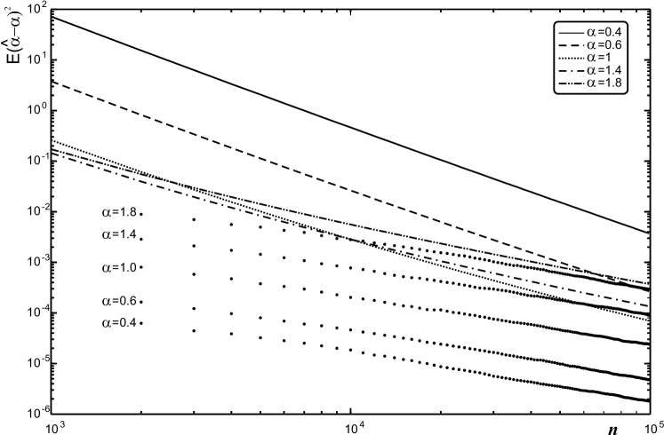
Figure 1: Evaluation of the variance of the parameter $\hat{\alpha}$ estimate. Dots denote selected values of the parameter $\alpha$. The curves denote the results of calculation by formula (5).

By substituting this estimate into (32), we derive the following inequality

$$|\tilde{\alpha}-\alpha|\leqslant\frac{|\tilde{\nu}-\nu|}{2\nu^{3/2}}+12(\tilde{\nu}-\nu)^{2}.$$

Next, by squaring both sides of the inequality, we get

$$\mathsf{E}(\tilde{\alpha}-\alpha)^{2}\leqslant\frac{\mathsf{E}(\tilde{\nu}-\nu)^{2}}{4\nu^{3}}+\frac{12}{\nu^{3/2}}\mathsf{E}|\tilde{\nu}-\nu|^{3}+144\mathsf{E}\left(\tilde{\nu}-\nu\right)^{4}.$$ (33)

By substituting (31), (30) and $(\ref{eq:nu_4moment})$ into (33) we get the theorem.

The results of the theorem were used for calculation of sample variance of the parameter $\alpha$. Algorithm of Kanter (1975) was used for the modelling of the stable random variables. Using this algorithm, we simulated the sample $X_{1},X_{2},\dots,X_{n}$ of the independent stable distributed random variables with predefined values of the parameters $\alpha,\beta,\theta,\gamma$. We constructed the estimate $\tilde{\alpha}$ and calculated the empirical variance of this estimate. This results of calculation are presented in Fig. 1. Here dots denote the empirical variance of the estimate $\tilde{\alpha}$ for the values of this parameter shown in the figure. Curved liens denote the results given by Theorem 1.1. This figure illustrates that the increasing of the parameter $\alpha$ leads to improved variance estimate, obtained from Theorem 1.1.

4 Approximation of the local fluctuation fluxes by the stable laws

In the investigation of local fluctuation fluxes in the edge region of plasma, investigators face the fact that the distribution densities of the amplitude of measurable fluctuation have heavy tails and acute vertices. This fact is described in many work (see, e.g. Carreras, van Milligen, Hidalgo et al. (1999); Sattin, Vianello, Valisa et al. (2005); Hidalgo C., Gonçalves B., Pedrosa M. A. et al. (2002); Skvortsova, Korolev, Maravina et al. (2005); Carreras, Hidalgo, Sanchez et al. (1996); Budaev, Takamura, Ohno et al. (2006); Zweben, Boedo, Grulke et al. (2007)). As a rule, these works state the fact on the presence of heavy tails of distributions, study the kurtosis and skewness coefficients Labit, Furno, Fasoli et al. (2007), and some of them make some assumptions on self-similarity of distributions obtained by different facilities Pedrosa, Hidalgo, Carreras et al. (1999). The presence of heavy tails and self-similarity of distributions leads to the idea of applying stable laws to approximation of their description.

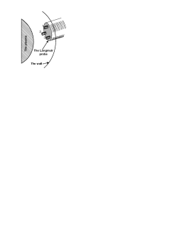
Figure 2: The experiment scheme in the fluctuation flux mesuarment.

A local fluctuation flux in the radial direction is defined as

$$\tilde{\Gamma}=\delta n_{e}\delta v_{r},$$ (34)

where $\delta n_{e}$ are fluctuations of plasma densities, $\delta v_{e}=c\delta E_{\theta}/B$ are fluctuations of radial velocity, $\delta E_{\theta}=(\delta\varphi_{1}-\delta\varphi_{2})/\Delta\theta r$ are fluctuations of a poloidal electric field, $\delta\varphi$ are fluctuations of floating potential, $\theta$ is a poloidal coordinate, and $r$ is the mean radius of magnetic surface.

Measurements were made on the stellarator L-2M. This is a dual-lead stellarator, the major radius of the torus $R=100$ cm., and the mean minor radius is $\langle r\rangle=11.5$ cm. The plasma was produced and heated by electron-cyclotron heating (ECH) regime at the second harmonic gyromagnetic frequency of the electron. The magnetic filed in the central region of the plasma was $B=1.3-1.4$ T. The gyrotron radiation power was $P_{0}=150-200$ kW, and the duration of the microwave impulse was 10-12 msec. The measurements were made in the plasma with average densities $\langle n\rangle=(1.3-1.8)\cdot 10^{13}\ cm^{-3}$, and the central electron temperature was $T_{e}(0)=0.6-1.0$ keV. The hydrogen was used as a plasma-forming gas. In the edge plasma, with the radius $r/r_{s}=0.9$ (where $r_{s}$ is a separatrix radius), the density was at the level of $n(r)=(1-2)\cdot 10^{12}\ cm^{-3}$, the electron temperature was $T_{e}(r)=30-40$, the relative density fluctuation range in the edge region of plasma was $(\delta n/n)_{\scriptsize out}=0.2-0.25$, and in the inner plasma region it was at the level $(\delta n/n)_{\scriptsize in}=0.1$.

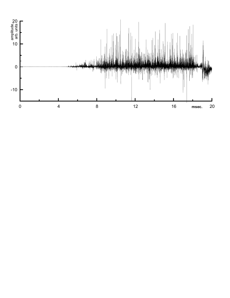
Figure 3: The typical signal of the local fluctuation flux in the radial direction.

The local fluctuation flux measurements were made by means of a three-pin Langmuir probe. The experiment scheme is presented in Fig. 2. The probe is located in a peripheric region of the plasma. The floating potential fluctuations $\delta\varphi_{1}$ and $\delta\varphi_{2}$ at the two neighboring points are measured by probes 1 and 2. The plasma density fluctuation $\delta n_{e}$ is measured by probe 3. Next, the local fluctuation flux is calculated by formula (34). A typical measuring signal is showed in Fig. 3. The time from the beginning of the signal is put off in the X-direction, and the time is measured in msec. The plasma appears in 8 msec. and disappear in 16 msec. We shall investigate namely this time interval (from 8 msec. to 16 msec.).

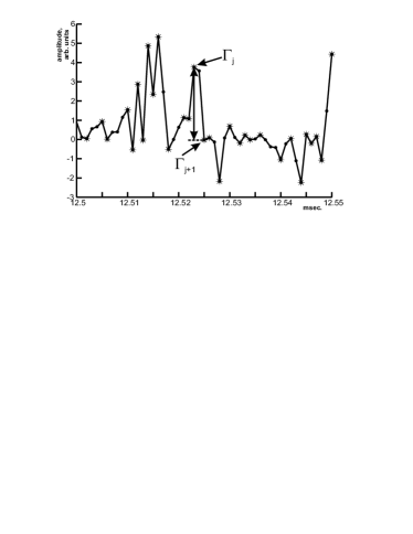
Figure 4: The signal is showed in Fig. 3 and plotted in the limits 12.5 - 12.55 msec.

Before applying the algorithm in statistical parameter estimation, we must be sure of independence of random variables that form a sample. Let us analyse the signal under consideration on an enlarged scale. The investigated signal is showed in Fig. 4 in the time interval from 12.5 msec. to 12.55 msec. Here dots denote flux values, which were written by the analog-digital convertor. The signal was quantized at the frequency 1 MHz. The figure illustrates that despite that the signal is very irregular, the trace of the increasing and decreasing intervals of the signal is considered. It means that the function depicted in Fig. 3 has a derivative, and, consequently, the successive points that describe an increase and a decrease in the flux are not independent. The dependence of investigated values does not allow us to use the algorithm of statistical estimation of parameters, because the proposition on statistical independence of random variables that form a sample, makes the basis of this algorithm. In order to use the algorithm, we have to exclude dependent values from the sample.

We proceed in the following way. Let us have a time series of the flux values $\tilde{\Gamma}_{i},\ i=1,\dots,N$, where $N$ is the total number of points in the signal. We select from the time series only those values which correspond to a maximum or a minimum of the flux. As a result, we get another time series which we denote as $\tilde{\Gamma}_{j},\ j=1,\dots,n$ and $n<N$. In Fig. 4, these points are denoted by an asterisk. We exclude all the other points from consideration. Next, we calculate increments between two successive values of the maximum and minimum $\Delta\tilde{\Gamma}_{k}=\tilde{\Gamma}_{j+1}-\tilde{\Gamma}_{j}$, where $k=1,\dots,n-1$.

Thus, we got a sample $\tilde{\Gamma}_{k}$. We suppose that the random variables in the sample $\tilde{\Gamma}_{k}$ are independent and have a stable distribution with the characteristic exponent $\alpha$. Let us apply the algorithm of statistical parameter estimation to this sample, which was described in section 2, and compare the probability density function of this sample with the probability density function of the stable law with the parameters $\tilde{\alpha},\tilde{\beta},\tilde{\lambda}$. The results of comparison are presented in Fig. 5. Here, the solid line denotes the density of stable law. As in the estimation we have got the value of the parameter $\beta=0$, we used the algorithm described in Uchaikin & Saenko (2002) for calculating the density of stable law. The figures illustrates that a slope of the tail of the stable law as $x\to\infty$ is coincident with the slope of the tail of the experimental density for flux amplitudes. It means that the characteristic exponent of the stable law is estimated correctly. Also, we can infer from the form of densities that the increments of amplitudes of local fluctuation fluxes in the peripheral region of plasma can be described by stable laws.

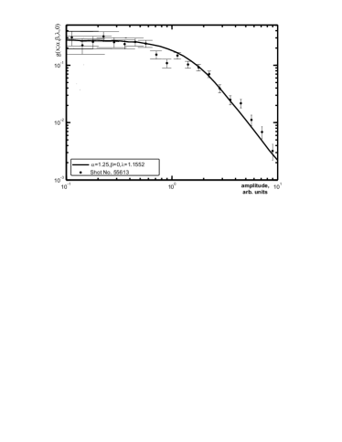
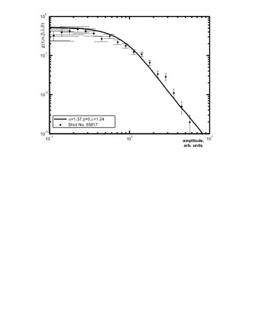
Figure 5: Description of the probability density function of amplitudes of fluctuation fluxes by stable laws for discharge No. 55613 (on the left) and No. 55617 (on the right). Here dots denote the empirical density of amplitude increments of fluctuation fluxes, solid lines denote the theoretical density of the stable law.

5 Conclusion

The estimate of a root-mean-square deviation of the characteristic exponent of stable law has been found. The comparison of the obtained estimation of root-mean-square deviation with the sample variance of the parameter $\alpha$ has showed that, by increasing the value of the parameter $\alpha$ the estimate of root-mean-square deviation is improved. It is possible to use this estimate for calculating of the variance of the parameter $\alpha$ with the values $\alpha\geqslant 1.5$.

Also stable laws were used to describe fluctuation fluxes in the peripherical region of plasma. The reason for their application is the fact that experimental distribution densities of the flux amplitude have heavy tails and sharp peaks. Therefore the normal distribution could not describe these distributions. The calculation has shown that probability density distributions of amplitudes of fluctuation fluxes are well described by stable laws. The coincidence of the tail slope of empirical and theoretical densities may serve as a corroboration of this result. Application of $\xi^{2}$ or Kolmogorov-Smirnov goodness-of-fit tests is rather difficult. The point is that densities of stable laws are calculated by the Monte-Carlo method and therefore the density values contain a statistical error, which has a negative influence on the result of the test.

References

- Budaev, Takamura, Ohno et al. (2006) Budaev, V., Takamura, S., Ohno, N. & Masuzaki, S. (2006). Superdiffusion and multifractal statistics of edge plasma turbulence in fusion devices. Nuclear Fusion 46, S181–S191. URL http://stacks.iop.org/0029-5515/46/S181.
- Carreras, Hidalgo, Sanchez et al. (1996) Carreras, B.A., Hidalgo, C., Sanchez, E., Pedrosa, M.A., Balbin, R., Garcia-Cortes, I., van Milligen, B., Newman, D.E. & Lynch, V.E. (1996). Fluctuation-induced flux at the plasma edge in toroidal devices. Physics of Plasmas 3, 2664–2672. 10.1063/1.871523. URL http://link.aip.org/link/?PHP/3/2664/1.
- Carreras, van Milligen, Hidalgo et al. (1999) Carreras, B.A., van Milligen, B., Hidalgo, C., Balbin, R., Sanchez, E., Garcia-Cortes, I., Pedrosa, M.A., Bleuel, J. & Endler, M. (1999). Self-similarity properties of the probability distribution function of turbulence-induced particle fluxes at the plasma edge. Phys. Rev. Lett. 83, 3653–3656. 10.1103/PhysRevLett.83.3653.
- Hidalgo C., Gonçalves B., Pedrosa M. A. et al. (2002) Hidalgo C., Gonçalves B., Pedrosa M. A., Castellano J., Erents K., Fraguas A. L., Hron M., Jiménez J. A., Matthews G. F., van Milligen B. & Silva C. (2002). Empirical similarity in probability density function of turbulent transport in the edge plasma region in fusion plasmas. Plasma Physics and Controlled Fusion 44, 1557–1564.
- Kanter (1975) Kanter, M. (1975). Ann. Probab. 3, 697.
- Labit, Furno, Fasoli et al. (2007) Labit, B., Furno, I., Fasoli, A., Diallo, A., Muller, S.H., Plyushchev, G., Podesta, M. & Poli, F.M. (2007). Universal statistical properties of drift-interchange turbulence in TORPEX plasmas. Physical Review Letters 98, 255002. 10.1103/PhysRevLett.98.255002. URL http://link.aps.org/abstract/PRL/v98/e255002.
- Pedrosa, Hidalgo, Carreras et al. (1999) Pedrosa, M.A., Hidalgo, C., Carreras, B.A., Balbín, R., García-Cortés, I., Newman, D., van Milligen, B., Sánchez, E., Bleuel, J., Endler, M., Davies, S. & Matthews, G.F. (1999). Empirical similarity of frequency spectra of the edge-plasma fluctuations in toroidal magnetic-confinement systems. Phys. Rev. Lett. 82, 3621–3624. 10.1103/PhysRevLett.82.3621.
- Sattin, Vianello, Valisa et al. (2005) Sattin, F., Vianello, N., Valisa, M., Antoni, V. & Serianni, G. (2005). On the probability distribution function of particle density and flux at the edge of fusion devices. Journal of Physics: Conference Series 7, 247–252. URL http://stacks.iop.org/1742-6596/7/247.
- Skvortsova, Korolev, Maravina et al. (2005) Skvortsova, N.N., Korolev, V.Y., Maravina, T.A., Batanov, G.M., Petrov, A.E., Pshenichnikov, A.A., Sarksyan, K.A., Kharchev, N.K., Sanchez, J. & Kubo, S. (2005). New possibilities for the mathematical modeling of turbulent transport processes in plasma. Plasma Physics Reports 31, 57–74.
- Uchaikin & Saenko (2002) Uchaikin, V.V. & Saenko, V.V. (2002). Simulation of random vectors with isotropic fractional stable distributions and calculation of their probability density function. J. Math. Sci. 112, 4211– 4228.
- Yanushkevichiene (1981) Yanushkevichiene, O. (1981). Investigation of some parameters of stable laws. Lietuvos matematikos rinkinys 21, 195–209.
- Zolotarev (1986) Zolotarev, V.M. (1986). One-dimensional stable Distributions. Amer. Mat. Soc., Providence, RI.
- Zweben, Boedo, Grulke et al. (2007) Zweben, S.J., Boedo, J.A., Grulke, O., Hidalgo, C., LaBombard, B., Maqueda, R.J., Scarin, P. & Terry, J.L. (2007). Edge turbulence measurements in toroidal fusion devices. Plasma Physics and Controlled Fusion 49, S1–S23. URL http://stacks.iop.org/0741-3335/49/S1.