Testing cosmological models with the brightness profile of distant galaxies

Abstract

The goal of this work is to use observed galaxy surface brightness profiles at high redshifts to determine, among a few candidates, the cosmological model best suited to interpret these observations. Theoretical predictions of galactic surface brightness profiles are compared to observational data in two cosmological models, $\Lambda$CDM and Einstein-de Sitter, to calculate the evolutionary effects of different spacetime geometries in these profiles in order to try to find out if the available data is capable of indicating the cosmology that most adequately represents actual galactic brightness profiles observations. Starting from the connection between the angular diameter distance and the galactic surface brightness as advanced by Ellis and Perry (1979), we derived scaling relations using data from the Virgo galactic cluster in order to obtain theoretical predictions of the galactic surface brightness modeled by the Sérsic profile at redshift values equal to a sample of galaxies in the range $1.5\lesssim z\lesssim 2.3$ composed by a subset of Szomoru’s et al. (2012) observations. We then calculated the difference between theory and observation in order to determine the changes required in the effective radius and effective surface brightness so that the observed galaxies may evolve to have features similar to the Virgo cluster ones. Our results show that within the data uncertainties of this particular subset of galaxies it is not possible to distinguish which of the two cosmological models used here predicts theoretical curves in better agreement with the observed ones, that is, one cannot identify a clear and detectable difference in galactic evolution incurred by the galaxies of our sample when applying each cosmology. We also concluded that the Sérsic index $n$ does not seem to play a significant effect in the evolution of these galaxies. Further developments of the methodology employed here to test cosmological models are also discussed.

1 Introduction

Observational cosmology attempts to understand the large-scale matter distribution in the universe and its geometry by basically following two different methodologies. The first, known as the direct-manner, or data-driven, approach, seeks to describe what is actually observed without addressing the question of why we observe such an universe the way it is, whereas the theory-based, or model-based, one interprets the observations based on explanations that can produce the observed patterns (Ellis 2006).

The theory-based approach consists of assuming a model based on a spacetime geometry and then determines the values of the free parameters by comparing the theoretical predictions with astronomical observations of distant objects. Currently, the most accepted cosmological model, the $\Lambda$CDM cosmology, is based on this theory-based approach. It concludes that the universe is almost entirely made up of dark matter and dark energy, whose compositions are presently unknown.

The data-driven approach of observational cosmology claims that we are in principle capable of determining the spacetime geometry on the null cone by means of astrophysical observations, that is, using data available on the past null cone (Kristian & Sachs 1966; Ellis et al. 1985). One specific study that follows this direct manner methodology was advanced by Ellis & Perry (1979), who developed a very detailed discussion connecting the galactic brightness profiles with cosmological models. Their aim was to determine the spacetime geometry of the universe by measuring the angular diameter distance $d_{\scriptscriptstyle A}$, also known as area distance, of distant galaxies through their surface brightness photometric data. Such a task was, however, made very difficult due to lack of detailed knowledge about the structure and evolution of galaxies. To this day this difficulty still remains.

Here we propose a method for testing cosmological models partially based on Ellis & Perry (1979) methodology, but less ambitious than theirs. Our approach differs from these authors in the sense that we do not aim to determine the entire spacetime geometry from observations. Our goal is to seek consistency between detailed astronomical observations of quantities describing actual galactic structures as compared to their predictions made by a specific cosmological model. To be precise, we start by assuming a cosmological model and then discuss the consistency between the model’s predictions and actual observations of the surface brightness of distant galaxies and other related quantities. The idea is to obtain a glimpse of the structure and evolution of galaxies by means of observations of our local universe, identify observing parameters which, in principle, are cosmological-model independent, that is, independent of the spacetime geometry, and then assume that galactic scaling relations do not change significantly, say within $3\sigma$, with the redshift. In this way we could select distant galaxies that form a homogeneous class of objects, defined as a set of similar galactic properties which can be found at different galactic evolutionary stages, such as morphology, so that one can compare objects at different redshift values. This implies in assuming that the variations in the scaling relations are related to the variations in the intrinsic structural parameters of a previously selected homogeneous class of objects (Ellis et al. 1984). By starting with a cosmological model we are able to assess to what extent the assumed cosmology affects actual galaxy evolution modeling carried out in extragalactic astrophysics where some cosmological model, nowadays the $\Lambda$CDM, is implicitly assumed.

In this paper we address the first step in this approach of cosmological model testing using actual galactic data, whose basic methodology was briefly advanced elsewhere (Olivares-Salaverri & Ribeiro 2009, 2010). The purpose here is to verify if a sample of galactic brightness profiles vary with their predicted theoretical ones when one changes the cosmological model, that is, if surface brightness profiles are affected by the spacetime geometry. We adopt two distinct cosmologies, the $\Lambda$CDM and, for simplicity in this initial approach, the Einstein-de Sitter (EdS) model. We then calculate photometric scaling relations using the Virgo cluster galaxies by means of the Kormendy et al. (2009) data and use our theory to predict the galactic surface brightness at high redshift values in the two cosmological models, assuming that these scaling relations do not change with the redshift. We then compare these predictions with a subsample of high redshift galactic surface brightness data of Szomoru et al. (2012; from now on S12).

Our results show that the observed high-redshift galactic brightness profiles differ from the theoretically predicted ones obtained by assuming that they follow scaling relations derived from the Virgo cluster. Such a difference occurs when the theoretical results are obtained by using both cosmological models studied here. Therefore, for these galaxies to change their features to the ones found in the Virgo cluster, an intrinsic evolution must take place. Such an evolution is similar in both cosmological models. Consequently, our results do not allow us to conclude which of the adopted cosmologies produce more or less evolution or is more suitable to represent the process in which high redshift galaxies develop into local galaxies having scaling relations similar to the ones observed in the Virgo galactic cluster, at least as far the chosen particular subset of S12 galaxies is concerned.

The outline of the paper is as follow. In §2 we discuss cosmological distance measures and their connections to astrophysical observables and §3 shows how the surface brightness of cosmological sources are connected to those distance measures. We present in §4 the received surface brightness using the profile due to Sérsic (1968). In §5 we calculate two photometric scaling relations of the Virgo cluster so that the next section (§6) shows our comparison, using the two cosmologies assumed here, between the prediction of the surface brightness obtained by means of these scaling relations and the observations of S12 high redshift galaxies. In §7 we calculate in both cosmological models how galaxies whose redshift values are equal to the ones in our chosen subsample of S12 observations would have to evolve to end up with features similar to the galaxies in the Virgo cluster. Finally, in §8 we summarize the results and present our conclusions.

2 Cosmological distances

We start by considering that source and observer are at relative motion to one another. From the point of view of the source, the light beams that travel along future null geodesics define a solid angle $\mathrm{d}\Omega_{\scriptscriptstyle G}$ with the origin at the source and have a transverse section area $\mathrm{d}\sigma_{\scriptscriptstyle G}$ at the observer (Ellis 1971; see also Fig. 2 of Ribeiro 2005 where cosmological distances are also discussed in some detail).

The specific radiative intensity $F_{em}$ is the emitted, or intrinsic, radiation measured at the source in a unit 2-sphere $S_{unit}$ lying in the locally Euclidean space at rest with the source and centered at it, also assumed to radiate locally with spherical symmetry. It is related to the intrinsic source luminosity $L$ by,

$$L=\int_{S_{unit}}F_{em}{\mathrm{d}}\Omega_{\scriptscriptstyle G}=4\pi F_{em}.$$ (1)

Let us now define $F_{re}$ as the flux radiated by the source, but measured by an observer located at some future time $t_{0}$ relative to the source. This is, of course, the received flux in the area $\mathrm{d}\sigma_{\scriptscriptstyle G}$ at rest with the observer and implies a certain distance between source and observer, distance which is geometrically defined along a null curve in an expanding spacetime where both source and observer are located. Thus, the source luminosity is given by,

$$L=\int_{S_{\!\!phys}}(1+z)^{2}F_{re}{\mathrm{d}}\sigma_{\scriptscriptstyle G},$$ (2)

where $z$ is the redshift and $S_{\!\!phys}$ is the physical surface receiving the flux, e.g., a detector. The factor $(1+z)^{2}$ appears here because both source and observer have their geometrical locus in a curved and expanding spacetime (Ellis 1971). Now, it has long been known that the area law establishes that the source intrinsic luminosity is independent from the observer (Ellis 1971). Therefore, these two equations are equal, yielding,

$$L=\int_{S}F_{em}\;{\mathrm{d}}\Omega_{\scriptscriptstyle G}=\int_{S}(1+z)^{2}F_{re}\;{\mathrm{d}}\sigma_{\scriptscriptstyle G},$$ (3)

$$F_{em}\;{\mathrm{d}}\Omega_{\scriptscriptstyle G}=const=(1+z)^{2}F_{re}\;{\mathrm{d}}\sigma_{\scriptscriptstyle G}.$$ (4)

Considering the source’s viewpoint, we may define the galaxy area distance $d_{\scriptscriptstyle G}$ as (Ellis 1971; see also Fig. 2 of Ribeiro 2005),

$${\mathrm{d}}\sigma_{\scriptscriptstyle G}={d_{\scriptscriptstyle G}}^{2}{\mathrm{d}}\Omega_{\scriptscriptstyle G}.$$ (5)

Thus, equation (4) becomes,

$$F_{re}=\frac{F_{em}}{{d_{\scriptscriptstyle G}}^{2}(1+z)^{2}}=\frac{L}{4\pi}\frac{1}{{d_{\scriptscriptstyle G}}^{2}(1+z)^{2}}.$$ (6)

The factor $(1+z)^{2}$ can be understood as arising from (i) the energy loss of each photon due to the redshift $z$, and (ii) the lower measured rate of incoming photons due to time dilation (Ellis 1971). Since the galaxy area distance $d_{\scriptscriptstyle G}$ appearing in equation (6) cannot be measured as ${\mathrm{d}}\Omega_{\scriptscriptstyle G}$ is defined at the source, we need to change this equation into another one containing measurable quantities. This can be done as follows.

From the point of view of the observer, the light beams that travel along its past null geodesics leave the source and converge to the observer, defining a solid angle $d\Omega_{\scriptscriptstyle A}$ with the origin at the observer and having transverse section area $d\sigma_{\scriptscriptstyle A}$ at the source (Ellis 1971; see also Fig. 1 of Ribeiro 2005). Then we can define the angular diameter distance $d_{\scriptscriptstyle A}$ as being given by,

$${\mathrm{d}}\sigma_{\scriptscriptstyle A}={d_{\scriptscriptstyle A}}^{2}{\mathrm{d}}\Omega_{\scriptscriptstyle A}.$$ (7)

Now we can use the reciprocity theorem, due to Etherington (1933; see also Ellis 1971, 2007), to relate $d_{\scriptscriptstyle G}$ to $d_{\scriptscriptstyle A}$. This theorem is written as follows,

$${d_{\scriptscriptstyle G}}^{2}=(1+z)^{2}{d_{\scriptscriptstyle A}}^{2}.$$ (8)

Thus, it is now possible to connect the flux received by the observer and the angular diameter distance by combining equations (6) and (8), yielding

$$F_{re}=\frac{F_{em}}{{d_{\scriptscriptstyle A}}^{2}(1+z)^{4}}.$$ (9)

The received flux $F_{re}$ and the redshift $z$ are astronomically measurable quantities. So, if the angular diameter distance $d_{\scriptscriptstyle A}$ is somehow determined astronomically, or obtained from theory as a function of $z$, then the intrinsic flux $F_{em}$ and, therefore, the intrinsic luminosity $L$ are both determined for all redshifts.

3 Connection with the surface photometry of cosmological sources

As discussed in §2, equation (9) connects the received and emitted fluxes of sources located in a curved spacetime, but that expression is valid for point like sources. Galaxies, however, form extended sources of light and their characterization requires defining another quantity, the surface brightness, better suited to describe them. The received surface brightness $B_{re}$ is defined as the ratio between the received flux and the observed solid angle of the galaxy,

$$B_{re}\equiv\frac{F_{re}}{{\mathrm{d}}\Omega_{\scriptscriptstyle A}}.$$ (10)

Considering equations (7) and (9), this expression can be rewritten as,

$$B_{re}=\frac{F_{em}}{{\mathrm{d}}\sigma_{\scriptscriptstyle A}}\frac{1}{(1+z)^{4}}.$$ (11)

If we define the emitted surface brightness $B_{em}$ as the intrinsic flux of the source $F_{em}$ per area unit in the rest frame of the source, we have that

$$B_{em}\equiv\frac{F_{em}}{{\mathrm{d}}\sigma{\scriptscriptstyle A}}.$$ (12)

Thus, equation (11) in fact connects the received and emitted surface brightness, as follows,

$$B_{re}=\frac{B_{em}}{(1+z)^{4}}.$$ (13)

This expression is simply the Tolman surface brightness test for cosmological sources, showing that galactic surface brightness does not depend on the distance. This equation also shows that if there is no significant cosmological effects, that is, if source and observer are close enough to be considered at rest with one another and Newtonian approximation is valid, then the source redshift is not significant. In this case there is no cosmological contribution ($z\sim 0$) and $B_{re}=B_{em}$. This can be considered as a consequence of the Liouville theorem (Bradt 2004). It is also worth mentioning that several authors name the radiation measured by the observer as intensity $I$, and the radiation emitted by the source as surface brightness $B$, instead of terms adopted here, respectively, received surface brightness $B_{re}$ and emitted surface brightness $B_{em}$. This is often the case in texts where General Relativity is not considered.

Actual astronomical observations are carried out in observational bandwidths and, therefore, the equations discussed so far should take this fact into account. The specific received surface brightness $B_{re,\nu_{re}}$ gives the amount of radiation received by the observer per unit solid angle measured at the observer in the frequency range $\nu_{re}$ and $\nu_{re}+{\mathrm{d}}\nu_{re}$. Clearly $B_{re}=\int_{0}^{\infty}B_{re,\nu_{re}}{\mathrm{d}}\nu_{re}$. Considering equation (13), we have that,

$$B_{re,\nu_{re}}{\mathrm{d}}\nu_{re}=\frac{B_{em,\nu_{em}}}{(1+z)^{4}}\,{\mathrm{d}}\nu_{em},$$ (14)

where we had defined the specific emitted surface brightness as follows,

$$B_{em,\nu_{em}}=B_{em}J(\nu_{em}).$$ (15)

Here $J(\nu)$ is the galactic spectral energy distribution (SED) giving the proportion of radiation at each frequency, being normalized by the condition

$$\int_{0}^{\infty}J(\nu)\,{\mathrm{d}}\nu=1.$$ (16)

From our definitions it also follows that $B_{em}=\int_{0}^{\infty}B_{em,\nu_{em}}{\mathrm{d}}\nu_{em}$. We need now to relate the received and emitted frequencies. This is accomplished by the definition of the redshift,

$$\nu_{em}=\nu_{re}(1+z),$$ (17)

implying that the SED of the source is observed according to $J(\nu_{em})=J\left[\nu_{re}(1+z)\right]$ and equation (14) can be rewritten as follows,

$$B_{re,\nu_{re}}{\mathrm{d}}\nu_{re}=\frac{B_{em,\nu_{em}}}{(1+z)^{3}}\,{\mathrm{d}}\nu_{re}.$$ (18)

The variables in the equation above depend on some implicit parameters. In order to reveal these dependencies, let us start by assuming our galaxy as having spherical symmetry with space points defined by the radius $R$. Furthermore, if this galaxy has a circular projection in the celestial sphere, any angle $\alpha$ measured by the observer corresponds to the radius $R$ in the source by means of the angular diameter distance at a given redshift. Hence, we have that (see Ellis & Perry 1979, Fig. 1),

$$R(z)=d_{\scriptscriptstyle A}(z)\;\alpha.$$ (19)

This expression is in fact a simplification of Eq. (7) where area and solid angle are respectively approximated to length and angle so that $d_{\scriptscriptstyle A}$ can be estimated observationally (Ellis 1971, Ribeiro 2005). Indeed, it is used in observational cosmology tests under the name “angular diameter redshift relation” since the angular diameter distance has all cosmological information. So, different values of the angular diameter distance are related to different cosmological models. As mentioned above, in this paper the two chosen cosmological models are EdS and $\Lambda$CDM.

The EdS cosmology has zero curvature and no cosmological constant so, in this model the angular diameter distance may be written as below,

$$d_{\scriptscriptstyle A,EdS}(z)=\frac{2c}{H_{0}(1+z)}\biggl{[}1-\frac{1}{\sqrt{(1+z)}}\biggr{]},$$ (20)

where $c$ is the light speed and $H_{0}$ is the Hubble constant. This expression shows that $d_{\scriptscriptstyle A,EdS}$ reaches a maximum value at $z=1.25$ and then starts decreasing, asymptotically vanishing at the big bang singularity hypersurface.

In the case of the $\Lambda$CDM model, several tests have been carried out in the last few years to measure the parameter values of the model leading to such a degree of accuracy that it became known as the concordance model, being the most accepted cosmology nowadays. Those tests involve studies of the cosmic microwave background radiation, baryonic acoustic oscillations and type Ia supernovae. Komatsu et al. (2009) presented values for several parameters in this cosmology to a high degree of accuracy, such as $H_{0}=71.8$ km s^-1 Mpc^-1, $\Omega_{m_{0}}=0.273$ and $\Omega_{\Lambda}=0.727$. We used these values to calculate numerically the angular diameter distance in both cosmologies, that is, $d_{\scriptscriptstyle A,\Lambda CDM}$ and $d_{\scriptscriptstyle A,EdS}$, where the latter is evaluated directly from equation (20).

Returning to equation (18), other implicit parameter dependence also occurs in both specific surface brightness. The received one depends on the observed parameters $\alpha$, $z$ and $\nu_{re}$, so that we should write it as $B_{re,\nu_{re}}=B_{re,\nu_{re}}(\alpha,z)$. The specific emitted surface brightness depends on the source parameters $R$, $\nu_{em}$ and, if allowed for the intrinsic evolution of the source, also in the $z$. Thus, $B_{em,\nu_{em}}=B_{em}(R,z)\,J[\nu_{re}(1+z),R,z]$. With these dependencies, equation (18) turns out to be written as the expression below (Ellis & Perry 1979),

$$B_{re,\nu_{re}}(\alpha,z)=\frac{B_{em}(R,z)}{(1+z)^{3}}\,J\left[\nu_{re}(1+z),R,z\right].$$ (21)

Note that this equation is completely general, i.e., valid for any cosmological model.

Next we shall show how the surface brightness $B_{em}(R,z)$ can be characterized by means of the Sérsic (1968) profile and obtain an explicit expression for the received surface brightness.

4 Received Sérsic surface brightness

The Sérsic profile was not commonly considered among astronomers after its proposal. Gradually, however, some authors started to claim that the Sérsic index is not simply a parameter capable of providing a better mathematical fit, but that it does have a physical meaning (Ciotti 1991; Caon et al. 1993; D’Onofrio et al. 1994). Nowadays, this profile seems to be more accepted since one can find in the recent literature several papers using it as well as relating its parameters to other astrophysical quantities (Davies et al. 1988; Prugniel & Simien 1997; Ciotti & Bertin 1999; Trujillo et al. 2001; Mazure & Capelato 2002; Graham 2001, 2002; Graham & Driver 2005; La Barbera et al. 2005; Coppola et al. 2009; Chakrabarty & Jackson 2009; Laurikainen et al. 2010). In view of this, we believe that this profile is the most suitable for the purposes of this paper.

The Sérsic profile can be presented in two slightly different parametric formats, although both of them characterize the same brightness profile. The difference lies in the interpretation of the parameters. The first one can be written as,

$$B_{\mathrm{S_{1}},em}(R,z)=B_{0}(z)\,\exp\left\{-\left[\frac{R(z)}{a(z)}\right]^{1/n}\right\},$$ (22)

where $B_{0}$ is the brightness amplitude, $a$ is the scalar radius and $n$ is the Sérsic index. Ellis & Perry (1979) implicitly used this form. The second way of writing the Sérsic profile is given by the following expression,

$$B_{\mathrm{S_{2}},em}(R,z)=B_{eff}(z)\,\exp\left\{\displaystyle-b_{n}\left[\left(\frac{R(z)}{R_{eff}(z)}\right)^{1/n}-1\right]\right\},$$ (23)

where $R_{eff}(z)$ is the effective radius, $B_{eff}(z)$ is the brightness at the effective radius and $b_{n}$ is a parameter dependent on the value of $n$.

The main difference between these two equations is the nature of their parameters. In equation (22) $B_{0}$ and $a$ do not have a clear physical meaning, whereas the parameters $B_{\scriptscriptstyle{eff}}$ and $R_{\scriptscriptstyle{eff}}$ appearing in equation (23) are more easily interpreted. $R_{\scriptscriptstyle{eff}}$ is defined as the isophote that contains half of the total luminosity and $B_{\scriptscriptstyle{eff}}$ is the value of the brightness in that radius (Ciotti 1991; Caon et al. 1993). For this reason we believe that the second form above is more appropriate for our analysis and we shall use it from now on.

A relationship between the different parameters in equations (22) and (23) can be obtained by equating these two expressions, yielding,

$$B_{0}(z)=B_{\scriptscriptstyle eff}(z)\,e^{b_{n}},$$ (24)

$$a(z)=\frac{R_{\scriptscriptstyle eff}(z)}{{b_{n}}^{n}}.$$ (25)

The evolution of the galactic structure is implicit in this profile in view of the fact that both $B_{eff}(z)$ and $R_{eff}(z)$ are redshift dependent. In addition, the connection of this profile to a cosmological model and, therefore, to the underlying curved spacetime geometry and its evolution occurs in the intrinsic radius $R(z)$ by means of equation (19). Thus, galaxies can possibly experience two simultaneous evolutionary effects, intrinsic source evolution and cosmological, or geometrical, evolution. Since at our current knowledge of galactic structure both effects cannot be easily separated, if they can be separated at all, from now on we shall assume that $R(z)$ depends only on the underlying spacetime geometry given by a chosen cosmological model. Furthermore, at first we shall not consider a possible intrinsic evolution of the Sérsic index in the form $n=n(z)$, because we assume that its change is produced via galactic merger processes (Naab & Trujillo 2006). So, the way that the evolutionary dependency is defined in the emitted surface brightness (Eq. 23) means that we are implicitly considering galaxies belonging to a set with similar properties, or a homogeneous class of objects. Departures from this class occur by smooth dependency in the evolution of the intrinsic parameters such as $B_{eff}(z)$ and $R_{eff}(z)$ (Ellis et al. 1984).

Let us now return to the properties of the Sérsic profile. There are analytical and exact expressions relating to $b_{n}$ and $n$. Analytical expressions for $b_{n}$ were given by several authors (Capaccioli 1989; Ciotti 1991; Prugniel & Simien 1997), whereas others worked out exact values for this parameter (Ciotti 1991; Graham & Driver 2005; Mazure & Capelato 2002). Ciotti & Bertin (1999) analyzed the exact value form and concluded that a fourth order expansion is enough to obtain good results, which are even better than the values obtained from the analytical expressions. Such an expansion is enough for the purposes of this paper and may be written as below,

$$b_{n}=2n-\frac{1}{3}+\frac{4}{405n}+\frac{46}{25515n^{2}}.$$ (26)

Having expressed $B_{em}$ in terms of the Sérsic profile, we can now obtain the equation for the received surface brightness $B_{re}(\alpha,z)$ since equation (21) gives the relationship between the emitted and received surface brightness. Considering the emitted brightness as modeled by the second form of the Sérsic profile (Eq. 23), we then substitute the latter equation into the former and obtain the following expression,

$$B_{re,\nu_{re}}(\alpha,z) = \frac{B_{eff}(z)}{(1+z)^{3}}\;J[\nu_{re}(1+z),R,z]\times$$ (27)

$$\times\exp{\left\{-b_{n}\left[{\left(\frac{R(z)}{R_{eff}(z)}\right)}^{1/n}-1\right]\right\}}.$$

Let us now define two auxiliary quantities required to study this problem from an extragalactic point of view (Caon et al. 1993; Graham & Driver 2005),

$$\mu_{re,\nu_{re}}(\alpha,z)\equiv-2.5\log\left(B_{re,\nu_{re}}\right),$$ (28)

$$\mu_{eff}(z)\equiv-2.5\log\left[B_{eff}(z)\right].$$ (29)

Equation (28) is given in units of $[\mu_{re,\nu_{re}}]$ = [mag/arc sec²]. Considering these definitions, equation (27) can be rewritten as follows,

$$\mu_{re,\nu_{re}}(\alpha,z) = \mu_{eff}(z)+7.5\log(1+z)$$ (30)

$$-2.5\log\left\{J\left[\nu_{re}(1+z),R,z\right]\right\}$$

$$+\left[\frac{2.5}{\ln(10)}\right]b_{n}\left\{\left[\frac{R(z)}{R_{eff}(z)}\right]^{1/n}-1\right\}.$$

This expression allows us to predict the galactic surface brightness in a given redshift and in a specific cosmological model. Nevertheless, in order to relate this expression with actual observations, we still need further assumptions regarding galactic structure. Next we shall make use of Kormendy et al. (2009) data to derive photometric scaling relations of the Virgo galaxy cluster and suppose that these relations do not change drastically out to the redshift range under study here.

5 Photometric scaling relations of the Virgo Cluster

In order to compare theoretical predictions of the surface brightness profiles with observational data we require information regarding the galactic structure, information which can be obtained after investigating scaling relations that different kinds of galaxies follow in the local universe. The most well-known of those relations are the ones that relate luminosity with velocity dispersion, such as the Faber-Jackson relation (Faber & Jackson 1976) for elliptical galaxies, and the Tully-Fisher relation (Tully & Fisher 1977) for spiral galaxies. Another, more general, scaling relation is the fundamental plane (Djorgovski & Davis 1987) which correlates velocity dispersion with effective brightness and effective radius instead of the luminosity. It is worth mentioning that the fundamental plane is a generalization of the Kormendy relation (Kormendy 1977).

The parameters involved in these scaling relations are measured through spectroscopic and photometric techniques. After knowing that the Sérsic index and the velocity dispersion correlate, a fundamental plane that only uses photometric parameters was proposed by Graham (2002). This variant, called photometric plane, uses parameters which appear in the definition of the Sérsic profile, i.e., the Sérsic index $n$, the effective surface brightness $\mu_{eff}$ and the effective radius $R_{eff}$. Since the study presented in this paper deals with photometric parameters, we shall use the photometric plane to obtain the galactic scaling relations required in our analysis. Specifically, our focus will be on the galaxies belonging to the Virgo cluster as their data (Kormendy et al. 2009) form the most exhaustively studied galactic surface brightness dataset in the local Universe.

5.1 Virgo cluster data

Kormendy et al. (2009) studied 42 galaxies of the Virgo cluster on the V band, $\lambda_{V,eff}=(5450\pm 880)$ Å, whose morphological types are elliptic (E), lenticular (S0) and spheroid (Sph). They used the Sérsic profile to fit the observed surface brightness and, in the authors’ words, “the Sérsic functions fit the main parts of the profiles of both elliptical and spheroidal galaxies astonishingly well on large ranges in surface brightness.”

As the observed data of the Virgo cluster is well fitted by the Sérsic profile, the parameters obtained through these fittings can be considered as reliable. Thus, using the parameters involved in the photometric plane, $n$, $\mu_{eff}$ and $R_{eff}$, we carried out linear fittings relating $\mu_{eff}$ to $n$ and $R_{eff}$ to $n$. Plots showing these fittings are presented in Fig. 1 and the fitted parameters are as follows,

$$\mu_{eff,V}=(0.38\pm 0.09)n+(20.5\pm 0.5),$$ (31)

$$\log R_{eff,V}=(0.21\pm 0.03)n-(0.5\pm 0.1).$$ (32)

The index $\scriptstyle V$ stands for the Virgo cluster.

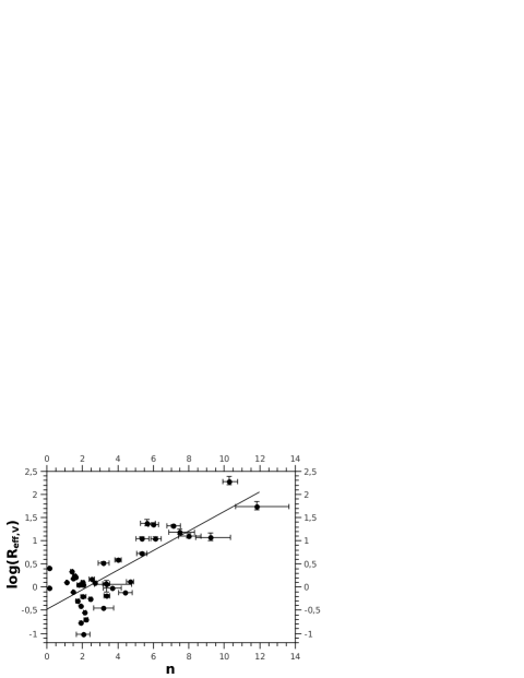
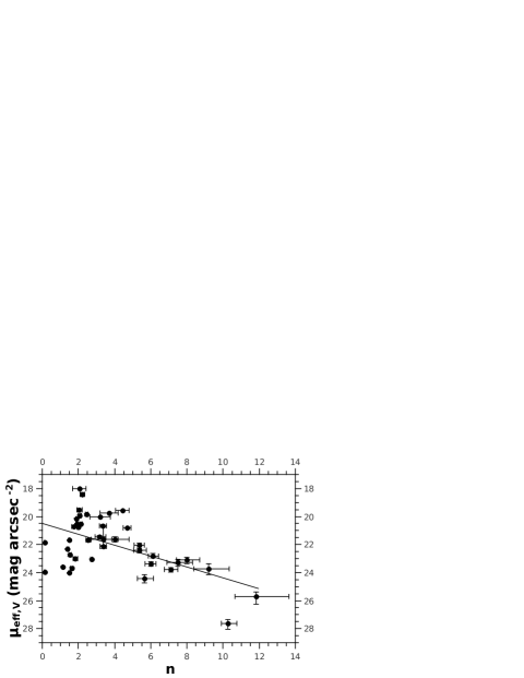
Figure 1: Left: Plot of the logarithm of the effective radius $R_{eff,V}$ vs. the Sérsic index $n$ of galaxies from the Virgo cluster. The straight line represents the linear fit whose values are given in eq. (32). Right: Plot of the effective brightness $\mu_{eff,V}$ and the Sérsic index $n$ of galaxies belonging to the Virgo cluster. The straight line represents the linear fit whose values are given in eq. (31). Both: Data taken from Kormendy et al. (2009).

Analyzing the plots we can observe that most galaxies with low Sérsic index do not correlate. These galaxies are mostly of spheroidal types and are the main contributors to the large errors in the Y-axis. As our aim is to compare the prediction of the surface brightness with high-redshift observational data, if we knew the morphological types of these high-redshift galaxies we could select specific galaxy types to obtain the scaling relation. But, this is usually not possible because galactic morphology at high redshifts is not as well established as in the local universe. Considering such constraint, we resorted on using galaxies of the Virgo cluster whose scaling relations were just derived in order to predict the surface brightness at any redshift and compare it with high redshift galaxy observations of S12. On top of the scaling relations, this is done by employing the two cosmological models adopted here.

6 High-redshift vs. predicted galactic surface brightness profiles in $\Lambda$CDM and EdS cosmologies

In order to analyze the possible effects that different cosmological models can have in the estimated galactic evolution, we shall compare theoretical predictions of the surface brightness data with high-redshift galactic brightness profiles. An important issue concerning high redshift galactic surface brightness is the depth in radius of these images. Observing the universe at high redshift involves lower resolution images, so obtaining a good sample of the brightness profiles as complete as possible in radius is not an easy task.

6.1 The high redshift galactic data of Szomoru et al. (2012)

S12 were mainly interested in investigating if the interpretation of the compactness of high redshift galaxies was due to a lack of deep images in radius which would lead to a misinterpretation of the compactness pattern. They observed a stellar mass limited sample of 21 quiescent galaxies in the redshift range $1.5<z<2.5$ having ${\cal{M}}_{*}>5.10^{10}{\cal{M}}_{\odot}$ and obtained their surface brightness using the Sérsic profile with high values in radius. We chose S12 data for our purposes mainly because of these features.

S12 used NIR data taken with HST WFC3 as part of the CANDELS survey. Specifically, the surface brightness profiles were obtained in the $H_{160}$ band, $\lambda_{H,eff}=(13923\pm 3840)$ Å, that is, comparable with the $V$ band rest-frame in the redshift range under consideration. From the 21 galaxies we have selected a subsample having Sérsic indexes grouped in three sets: $n\sim 1$, $n\sim 4$ and $n\sim 5$. The last two sets are more numerous and are located in several redshift values, especially the group with $n\sim 5$. Table LABEL:table1 shows our subsample with the identification number in the S12 catalog and their respective Sérsic indexes and the redshifts.

Table 1: Identification (ID) number, Sérsic index $n$ and redshift of the galaxy subsample selected from S12 and used in this paper.

ID	$n$	$z$
2.856	1.20 $\pm$ 0.08	1.759
3.548	3.75 $\pm$ 0.48	1.500
2.531	4.08 $\pm$ 0.30	1.598
3.242	4.17 $\pm$ 0.45	1.910
3.829	4.24 $\pm$ 1.15	1.924
1.971	5.07 $\pm$ 0.31	1.608
3.119	5.09 $\pm$ 0.60	2.349
6.097	5.26 $\pm$ 0.56	1.903
1.088	5.50 $\pm$ 0.67	1.752

6.2 Theoretical predictions of the surface brightness

As discussed above, equation (30) allows us to calculate the surface brightness theoretical prediction of a hypothetical galaxy in a given redshift. We have already calculated scaling relations for local galaxies which we assume to be maintained out to the observed S12 redshift values. However, to see if the observed high redshift galaxies behave like the Virgo cluster ones, i.e., if they obey the assumed scaling relations, we must calculate the errors of the theoretical predictions in Eq. (30).

Errors for $\Delta\mu_{re,\nu_{re}}$ are estimated quadratically as follows,

$$\Delta\mu_{re,\nu_{re}} = \biggl{[}\biggl{(}\frac{\partial\mu_{re,\nu_{re}}}{\partial\mu_{eff}}\Delta\mu_{eff}\biggr{)}^{2}+\biggr{(}\frac{\partial\mu_{re,\nu_{re}}}{\partial z}\Delta z\biggr{)}^{2}+\biggr{(}\frac{\partial\mu_{re,\nu_{re}}}{\partial n}\Delta n\biggr{)}^{2}$$ (33)

$$+\biggr{(}\frac{\partial\mu_{re,\nu_{re}}}{\partial R}\Delta R\biggr{)}^{2}+\biggr{(}\frac{\partial\mu_{re,\nu_{re}}}{\partial\log(R_{eff})}\Delta\log(R_{eff})\biggr{)}^{2}\biggl{]}^{1/2}.$$

Let us analyze individually each of the uncertainty terms in this expression.

6.2.1 $\Delta\mu_{eff}$

The effective surface brightness is calculated from the linear fit of the Virgo cluster galaxy scaling relation,

$$\mu_{eff}=A_{\mu_{eff}}n+B_{\mu_{eff}},$$ (34)

where $A$ and $B$ are the linear fit parameters given in equation (31). Its uncertainty yields,

$$\Delta\mu_{eff}=\biggl{[}\biggl{(}\frac{\partial\mu_{eff}}{\partial A_{\mu_{eff}}}\Delta A_{\mu_{eff}}\biggr{)}^{2}+\biggl{(}\frac{\partial\mu_{eff}}{\partial n}\Delta n\biggr{)}^{2}+\biggl{(}\frac{\partial\mu_{eff}}{\partial B_{\mu_{eff}}}\Delta B_{\mu_{eff}}\biggr{)}^{2}\biggr{]}^{1/2}.$$ (35)

This expression can can be rewritten as below,

$$\Delta\mu_{eff}=\biggl{[}(n\Delta A_{\mu_{eff}})^{2}+(A_{\mu_{eff}}\Delta n)^{2}+(\Delta B_{\mu_{eff}})^{2}\biggr{]}^{1/2},$$ (36)

where $\Delta A$ and $\Delta B$ come from the linear fit and $\Delta n$ comes from the observation.

6.2.2 $\Delta z$

Redshift uncertainty was given by S12 only if $z$ was measured photometrically. However, some of S12’s galaxies had their redshifts measured spectroscopically, then the errors were not made available. Since there is a mixture of photometric and spectroscopic redshifts in S12’s sample, we decided to avoid including them in our calculations and have effectively assumed $\Delta z\sim 0$.

6.2.3 $\Delta n$

The value of Sérsic index and its error came directly from the observations shown in S12 (see Table LABEL:table1).

6.2.4 $\Delta R$

The projected radius is obtained by means of equation (19), whose quadratic uncertainty may be written as follows,

$$\Delta R=\biggl{[}\biggl{(}\frac{\partial R}{\partial\alpha}\Delta\alpha\biggr{)}^{2}+\biggl{(}\frac{\partial R}{\partial d_{A}}\Delta d_{A}\biggr{)}^{2}\biggr{]}^{1/2}.$$ (37)

The angle uncertainty $\Delta\alpha$ was neglected by S12, so $\Delta\alpha\sim 0$. Regarding the angular diameter distance, the small uncertainties in the parameters of the cosmological models are such that once propagated they change very little the value of $d_{A}$. So, we effectively have $\Delta d_{A}\sim 0$.

6.2.5 $\Delta\log(R_{eff})$

Similarly to $\Delta\mu_{eff}$, the uncertainty $\Delta\log(R_{eff})$ is derived from the linear fit of the Virgo galaxy cluster,

$$\log(R_{eff})=A_{\log(R_{eff})}n+B_{\log(R_{eff})},$$ (38)

where $A$ and $B$ are the parameters given by equation (32). Therefore,

$$\Delta\log(R_{eff}) = \biggl{\{}\biggl{[}\frac{\partial\log(R_{eff})}{\partial A_{\log(R_{eff})}}\Delta A_{\log(R_{eff})}\biggr{]}^{2}+\biggl{[}\frac{\partial\log(R_{eff})}{\partial n}\Delta n\biggr{]}^{2}$$ (39)

$$+\biggl{[}\frac{\partial\log(R_{eff})}{\partial B_{\log(R_{eff})}}\Delta B_{\log(R_{eff})}\biggr{]}^{2}\biggr{\}}^{1/2},$$

which may be rewritten as,

$$\Delta\log(R_{eff})=\biggl{\{}\bigl{[}n\Delta A_{\log(R_{eff})}\bigr{]}^{2}+(A\Delta n)^{2}+\bigl{[}\Delta B_{\log(R_{eff})}\bigr{]}^{2}\biggr{\}}^{1/2}.$$ (40)

Just like in $\Delta\mu_{eff}$, $\Delta A_{\log(R_{eff})}$ and $\Delta B_{\log(R_{eff})}$ come from the linear fit and $\Delta n$ is given by observations.

6.2.6 $\Delta\mu_{re,\nu_{re}}$

Putting together all these expressions for uncertainties in equation (33) and remembering the relationship between $b_{n}$ and $n$ (Eq. 26), the uncertainty in the theoretical prediction of the surface brightness yields,

$$\Delta\mu_{re,\nu_{re}} = \Biggl{(}(n\Delta A_{\mu_{eff}})^{2}+(A_{\mu_{eff}}\Delta n)^{2}+(\Delta B_{\mu_{eff}})^{2}+$$ (41)

$$+\biggl{[}\biggl{(}\frac{2.5}{\ln 10}\frac{{\mathrm{d}}b_{n}}{{\mathrm{d}}n}\biggl{\{}\bigg{[}\frac{R}{10^{\log(R_{eff})}}\biggr{]}^{1/n}-1\biggr{\}}-$$

$$-\frac{2.5b_{n}}{n^{2}\ln 10}\biggl{[}\frac{R}{10^{\log(R_{eff})}}\biggr{]}^{1/n}\log\biggl{\{}\frac{R}{10^{\log(R_{eff})}}\biggr{\}}\biggr{)}\Delta n\biggr{]}^{2}+$$

$$+\biggl{\{}\frac{2.5b_{n}}{n}\biggl{[}\frac{R}{10^{\log(R_{eff})}}\biggr{]}^{1/n}\biggr{\}}^{2}\biggl{\{}[n\Delta A_{\log(R_{eff})}]^{2}+$$

$$+[A_{\log(R_{eff})}\Delta n]^{2}+[\Delta B_{\log(R_{eff})}]^{2}\biggr{\}}\Biggr{)}^{1/2}.$$

6.2.7 Comparing theory and observation

Before we can actually compare our S12 galaxy subsample with the theoretical predictions of the surface brightness profile, we still need to estimate the spectral energy distribution (SED) $J$. We proceed on this point from the very simple working assumption of a constant value for the SED, since using the overall energy distribution of the galaxies in the Virgo cluster in different bandwidths is beyond the aims of this paper. Henceforth, we assume the working value of $J=0.5$.

The scaling relations obtained from the galaxies of the Virgo cluster, Eqs. (31) and (32), allow us to calculate $\mu_{eff}$ and $R_{eff}$ for a given Sérsic index value. So, these two equations may be rewritten as,

$$\mu_{eff,V}=0.38n+20.5,$$ (42)

where its error is given by,

$$\Delta\mu_{eff,V}=0.09n+0.5,$$ (43)

and

$$\log R_{eff,V}=0.21n-0.5,$$ (44)

whose uncertainty is,

$$\Delta\log R_{eff,V}=0.03n+0.1.$$ (45)

Graphs showing the S12 data, labeled as “Obs”, and the theoretical predictions of the surface brightness profile, labeled as “Pre”, in each of the two cosmological models adopted in this work, $\Lambda$CDM and Einstein-de Sitter, are shown in Figs. 2 to 11. One can clearly see that the observed and predicted results are very different, a result which shows that the Virgo cluster galaxies do not behave as our S12 subsample. So, for our high redshift galaxies to evolve into the Virgo cluster ones the scaling relations parameters have to change in order to reflect such an evolution. One can also see that the difference in the results when employing each of the two cosmological models is not at all significant. Thus, our next step is to work out the changes in the parameter to find out if the evolution these galaxies have to sustain is strongly dependent on the assumed underlying cosmology.

Figure 2: Both: galaxy ID 2.856 from S12 labeled as “Obs” at $z=1.759$ with $n=1.2\pm 0.08$. Theoretical prediction using Eqs. (30) and (41) assuming the scaling relations of Virgo cluster galaxies, labeled as “Pre”. Left: Considering $\Lambda$CDM cosmological model. Right: Considering Einstein-de Sitter cosmological model.

Figure 3: Both: galaxy ID 2.531 from S12 labeled as “Obs” at $z=1.598$ with $n=4.08\pm 0.3$. Theoretical prediction using Eqs. (30) and (41) assuming the scaling relations of Virgo cluster galaxies, labeled as “Pre”. Left: Considering $\Lambda$CDM cosmological model. Right: Considering Einstein-de Sitter cosmological model.

Figure 4: Both: galaxy ID 3.242 from S12 labeled as “Obs” at $z=2.47$ with $n=4.17\pm 0.45$. Theoretical prediction using Eqs. (30) and (41) assuming the scaling relations of Virgo cluster galaxies, labeled as “Pre”. Left: Considering $\Lambda$CDM cosmological model. Right: Considering Einstein-de Sitter cosmological model.

Figure 5: Both: galaxy ID 3.548 from S12 labeled as “Obs” at $z=1.5$ with $n=3.75\pm 0.48$. Theoretical prediction using Eqs. (30) and (41) assuming the scaling relations of Virgo cluster galaxies, labeled as “Pre”. Left: Considering $\Lambda$CDM cosmological model. Right: Considering Einstein-de Sitter cosmological model.

Figure 6: Both: galaxy ID 3.829 from S12 labeled as “Obs” at $z=1.924$ with $n=4.24\pm 1.15$. Theoretical prediction using Eqs. (30) and (41) assuming the scaling relations of Virgo cluster galaxies, labeled as “Pre”. Left: Considering $\Lambda$CDM cosmological model. Right: Considering Einstein-de Sitter cosmological model.

Figure 7: Both: galaxy ID 1.088 from S12 labeled as “Obs” at $z=1.752$ with $n=5.5\pm 0.67$. Theoretical prediction using Eqs. (30) and (41) assuming the scaling relations of Virgo cluster galaxies, labeled as “Pre” points. Left: Considering $\Lambda$CDM cosmological model. Right: Considering Einstein-de Sitter cosmological model.

Figure 8: Both: galaxy ID 1.971 from S12 labeled as “Obs” at $z=1.608$ with $n=5.07\pm 0.31$. Theoretical prediction using Eqs. (30) and (41) assuming the scaling relations of Virgo cluster galaxies, labeled as “Pre”. Left: Considering $\Lambda$CDM cosmological model. Right: Considering Einstein-de Sitter cosmological model.

Figure 9: Both: galaxy ID 2.514 from S12 labeled as “Obs” at $z=1.548$ with $n=5.73\pm 0.93$. Theoretical prediction using Eqs. (30) and (41) assuming the scaling relations of Virgo cluster galaxies, labeled as “Pre”. Left: Considering $\Lambda$CDM cosmological model. Right: Considering Einstein-de Sitter cosmological model.

Figure 10: Both: galaxy ID 3.119 from S12 labeled as “Obs” at $z=2.349$ with $n=5.09\pm 0.6$. Theoretical prediction using Eqs. (30) and (41) assuming the scaling relations of Virgo cluster galaxies, labeled as “Pre”. Left: Considering $\Lambda$CDM cosmological model. Right: Considering Einstein-de Sitter cosmological model.

Figure 11: Both: galaxy ID 6.097 from S12 labeled as “Obs” at $z=1.903$ with $n=5.26\pm 0.56$. Theoretical prediction using Eqs. (30) and (41) assuming the scaling relations of Virgo cluster galaxies, labeled as “Pre”. Left: Considering $\Lambda$CDM cosmological model. Right: Considering Einstein-de Sitter cosmological model.

7 Evolution to the Virgo cluster scaling parameters in $\Lambda$CDM and EdS cosmologies

As seen above, the theoretical prediction of the surface brightness profiles obtained through scaling relations derived from data of the Virgo galactic cluster are very different from the observed surface brightness of S12 galaxies in both cosmological models studied here. Hence, in order to ascertain the possible evolution that these galaxies would have to experience such that they end up with surface brightness equal to the ones in the Virgo cluster, we need to look carefully at the parameter evolution of the scaling relations. Assuming that they do not evolve through the Sérsic index $n$ (see above), we can study such an evolution via the effective brightness and the effective radius.

Let $\mu_{eff,evo}$ and $\log R_{eff,evo}$ be, respectively, the evolution of the effective brightness and the effective radius. We can estimate these two quantities similarly to our previous calculation of the scaling relations. For values of the Sérsic index of our S12 galactic subsample, we can obtain their respective Virgo cluster galaxies effective brightness and effective radius $\mu_{eff,V}$ and $\log R_{eff,V}$ by means of the expressions (42) to (45). We then modify the linear fit parameters $A$ and $B$ in these expressions ($y=Ax+B$), adjusting them so that the results approximate the points of the theoretical predictions with S12’s observed values in order to find $\mu_{eff,Szo}$ and $\log R_{eff,Szo}$, that is, the values of effective brightness and effective radius of our subsample of S12’s galaxies. Therefore, both $\mu_{eff,evo}$ and $\log R_{eff,evo}$ are given as follows,

$$\mu_{eff,evo}=\mu_{eff,Szo}-\mu_{eff,V},$$ (46)

$$\log R_{eff,evo}=\log R_{eff,Szo}-\log R_{eff,V}.$$ (47)

The respective uncertainties yield,

$$\Delta\mu_{eff,evo}=\Delta\mu_{eff,Szo}+\Delta\mu_{eff,V},$$ (48)

$$\Delta\log R_{eff,evo}=\Delta\log R_{eff,Szo}+\Delta\log R_{eff,V}.$$ (49)

Table LABEL:table2 shows the effective brightness and effective radius for the Virgo cluster galaxies obtained with Sérsic indexes $n$ equal to those in our S12 subsample presented in Table LABEL:table1. These quantities were obtained using the Virgo scaling relations.

Table 2: Effective brightness $\mu_{eff,V}$ and effective radius $\log R_{eff,V}$ obtained with Virgo cluster galaxies scaling relations for values of $n$ equal to those in our subsample of S12 galaxies.

ID	$\mu_{eff,V}$	$\log R_{eff,V}$
2.856	21.0 $\pm$ 0.7	-0.3 $\pm$ 0.2
3.548	21.9 $\pm$ 0.9	0.3 $\pm$ 0.3
2.531	22.1 $\pm$ 0.9	0.4 $\pm$ 0.3
3.242	22.1 $\pm$ 0.9	0.4 $\pm$ 0.3
3.829	22.1 $\pm$ 0.9	0.4 $\pm$ 0.3
1.971	22 $\pm$ 1	0.6 $\pm$ 0.3
3.119	22 $\pm$ 1	0.6 $\pm$ 0.3
6.097	22 $\pm$ 1	0.6 $\pm$ 0.3
1.088	23 $\pm$ 1	0.6 $\pm$ 0.3

Table LABEL:table3 shows the same quantities for the adjusted parameters of our subsample of S12 galaxies using the two cosmological models considered here and Table LABEL:table4 presents the evolution of the effective brightness and effective radius calculated using eqs. (46) to (49) in both cosmological models in the V band.

Table 3: Effective brightness $\mu_{eff,Szo}$ and effective radius $\log R_{eff,Szo}$ of the adjusted parameters from the galaxies selected from S12 for values of $n$ equal to the ID galaxies in the V band in the two cosmological models considered in this paper.

ID	$\mu_{eff,Szo,\Lambda CDM}$	$\log R_{eff,Szo,\Lambda CDM}$	$\mu_{eff,Szo,EdS}$	$\log R_{eff,Szo,EdS}$
2.856	16.5 $\pm$ 0.6	-0.1 $\pm$ 0.1	16.7 $\pm$ 0.6	-0.1 $\pm$ 0.1
3.548	16.5 $\pm$ 0.8	-0.2 $\pm$ 0.3	16.4 $\pm$ 0.8	-0.3 $\pm$ 0.2
2.531	16.7 $\pm$ 0.9	0.0 $\pm$ 0.3	17.1 $\pm$ 0.9	-0.1 $\pm$ 0.3
3.242	14.9 $\pm$ 0.9	-0.4 $\pm$ 0.3	14.3 $\pm$ 0.9	-0.6 $\pm$ 0.3
3.829	18.1 $\pm$ 0.9	0.2 $\pm$ 0.2	17.1 $\pm$ 0.9	-0.1 $\pm$ 0.3
1.971	19.3 $\pm$ 0.9	0.5 $\pm$ 0.3	20 $\pm$ 1	0.5 $\pm$ 0.3
3.119	16 $\pm$ 1	-0.1 $\pm$ 0.3	16 $\pm$ 1	-0.3 $\pm$ 0.3
6.097	17 $\pm$ 1	0.3 $\pm$ 0.3	18 $\pm$ 1	0.3 $\pm$ 0.3
1.088	16 $\pm$ 1	17 $\pm$ 1	17 $\pm$ 1	-0.2 $\pm$ 0.3

Table 4: Evolution of the effective brightness $\mu_{eff,evo}$ and effective radius $\log R_{eff,evo}$ of the galaxies selected from S12 for values of $n$ equal to the ID galaxies in the V band in the two cosmological models considered here.

ID	$\mu_{eff,evo,\Lambda CDM}$	$\mu_{eff,evo,EdS}$	$\log R_{eff,evo,\Lambda CDM}$	$\log R_{eff,evo,EdS}$
2.856	-5 $\pm$ 2	-4 $\pm$ 2	0.2 $\pm$ 0.3	0.2 $\pm$ 0.3
3.548	-6 $\pm$ 2	-6 $\pm$ 2	-0.4 $\pm$ 0.4	-0.6 $\pm$ 0.5
2.531	-5 $\pm$ 2	-5 $\pm$ 2	-0.4 $\pm$ 0.5	-0.5 $\pm$ 0.5
3.242	-7 $\pm$ 2	-7 $\pm$ 2	-0.7 $\pm$ 0.5	-1.0 $\pm$ 0.4
3.829	-4 $\pm$ 2	-5 $\pm$ 2	-0.2 $\pm$ 0.3	-0.5 $\pm$ 0.5
1.971	-3 $\pm$ 2	-2 $\pm$ 2	0.0 $\pm$ 0.5	0.0 $\pm$ 0.5
3.119	-6 $\pm$ 2	-6 $\pm$ 2	-0.7 $\pm$ 0.5	-0.8 $\pm$ 0.5
6.097	-5 $\pm$ 2	-4 $\pm$ 2	-0.3 $\pm$ 0.5	-0.2 $\pm$ 0.5
1.088	-6 $\pm$ 2	-6 $\pm$ 2	-0.7 $\pm$ 0.6	-0.8 $\pm$ 0.6

The results show that the evolution that will have to occur so that the S12 high redshift galaxies have effective brightness and effective radius equal to the ones in the Virgo cluster is similar in both cosmological models. Specifically, it seems that in EdS model the effective radius evolution is higher than the one occurred in the $\Lambda$CDM model. Nevertheless, the evolution of the effective surface brightness is almost the same in both models. We also note that the difference in the Sérsic index values do not appear to affect our results, which also clearly show that the uncertainties in the measurements of both quantities we deal with here are just too high to allow us to distinguish the underlying cosmological model that best represents the data. Basically our methodology is limited by the uncertainties, at least as far as the S12 subset data is concerned.

As final words, this work is based on the assumption that the galaxies we compare belong to a group whose members share at least one common feature regardless of the redshift, otherwise comparison among them becomes impossible. In other words, our basic assumption is that our selected galaxies belong to a homogeneous class of galaxies. In the analysis we carried out above we grouped our galaxies using only the Sérsic indexes, this therefore being our defining criterion of a homogeneous class of objects. So, in a sense we followed Ellis & Perry (1979) and adopted morphology as our definition of a homogeneous class.

8 Summary and conclusions

In this paper we have compared high redshift surface brightness observational data with theoretical surface brightness predictions for two cosmological models, namely the $\Lambda$CDM and Einstein-de Sitter, in order to test if such comparison allows us to distinguish the cosmology that best fits the observational data. We started by reviewing the expressions for the emitted and received bolometric source brightness and then obtained their respective specific expressions in the context of galactic surface brightness (Ellis 1971; Ellis & Perry 1979).

Using the Sérsic profile, we have obtained scaling relations between the surface effective brightness $\mu_{eff}$ and Sérsic index, as well as between the effective radius $R_{eff}$ and $n$, for the Virgo cluster galaxies using Kormendy et al. (2009) data. Assuming this scaling relation, we have calculated theoretical predictions of the surface brightness and compared them with some of the observed surface brightness profiles of high-redshift galaxies in a subsample of Szomoru et al. (2012) galaxies in the two cosmological models considered here. Our results showed that although the Sérsic profile fits well the observed brightness, the results for surface brightness is different from the theoretical predictions. Such difference was used to calculate the amount of evolution that the high redshift galaxies would have to experience in order to achieve the Virgo cluster structure once they arrive at $z\sim 0$. We concluded from our results that the cosmological evolution is quite similar in the two models considered in this paper. We also noted that galaxies having different Sérsic indexes do not seem to follow a different evolutionary path.

Overall, with the data and errors available for the chosen subset of galactic profiles used here we cannot distinguish between the two different cosmological models assumed in this work. That is, assuming that the high redshift galaxies will evolve to have features similar to the ones found in the Virgo cluster, it is not possible to conclude which cosmological model will predict theoretical surface brightness curves similar to the observed ones due to the high uncertainties in the data used here. We also noted that the Sérsic index does not seem to play any significant evolutionary role, as the evolution we discussed is apparently not affected by the value of $n$. Nevertheless, this work used only the Sérsic index to define a homogeneous class of objects.

Considering that the results shown above depend on the chosen underlying cosmology it is reasonable to ask if the use of a different enough cosmological model will produce relatively large effects in the quantities analyzed here. On this regard, the most different cosmologies still capable of describing observed features of the Universe are the inhomogenous cosmological models (Bolejko 2006; Bolejko et al. 2011; Krasiński 2011; Hellaby and Walters 2018, and references therein). Those, however, come with much greater degrees of freedom as compared to the standard cosmology in the form of arbitrary functions which must be defined a priori in terms of some kind of presumably observable features, particularly mass distribution (Bolekjo et al. 2011, §4), which can be defined in such a way that the resulting model becomes an almost standard cosmology as far as some observables are concerned. This is the case of the simplest inhomogeneous model, the Lemaître-Tolman-Bondi (LTB) cosmology, whose arbitrary functions can be established in such a way that in some cases the final cosmology differs little in terms of some chosen observational features from the results obtained with the standard cosmology (e.g., Ribeiro 1993, Iribarrem et al. 2014, Lopes et al. 2017). If, however, one goes to more extreme inhomogeneous cosmologies specifications their high nonlinearity prevents us from reaching any conclusion beforehand. One has to actually carry out the calculations in order to see if there is any relative large effects in the quantities analyzed here.

The main point is that the intrinsic high nonlinearity of relativistic cosmological models may lead to different results for each observational quantity that is calculated. For instance, a particular LTB model that provides observational results similar to the standard model for a certain set of observations might end up producing entirely different ones for other set of observations. In addition, since it seems that no inhomogeneous model has so far been used to describe the problem discussed here, if and how much inhomogeneous cosmologies, LTB or otherwise, would affect the galactic surface brightness profiles in the form studied in this paper remains an open problem. Therefore, it seems that to start looking at this problem one has to choose a simple LTB model already used by other authors, which describes some basic observed features such as voids, and then carry out the calculations in order to draw comparisons.

Summing up those results, it seems reasonable that future studies of this kind should also select galaxies based on other features besides morphology in order to increase the number of common properties between high and low redshift galaxies, and, of course, using different data samples than those adopted here. More common features such as the Sérsic index are essential for a better definition of a homogeneous class of cosmological objects whose observational features are possibly able to distinguish among different cosmological scenarios. However, care should be taken to avoid features which can possibly suffer dramatic cosmological evolution.

Data Availability

All data generated or analysed during this study are included in this published article.

Competing Interests

The authors have no competing interests to declare that are relevant to the content of this article.

References

- Bolejko (2006) Bolejko, K. 2006, Proc. 13th Young Scientists’ Conference on Astron. & Space Phys., Kyiv, Ukraine; A. Golovin, G. Ivashchenko & A. Simon (eds), arXiv:astro-ph/0607130
- Bolejko et al. (2011) Bolejko, K., Célérier, M. N., & Krasiński, A. 2011, Class. Quantum Grav., 28, 164002, arXiv:1102.1449
- Bradt (2004) Bradt, H. 2004, Astronomy Methods: A Physical Approach to Astronomical Observations, UK: Cambridge University Press, 2004
- Caon, Capaccioli & D’Onofrio (1993) Caon, N., Capacccioli, M., & D’Onofrio, M. 1993, MNRAS, 265, 1013
- Capaccioli (1989) Capaccioli, M. 1989, in World of Galaxies, eds. H.G. Corwin Jr. & L. Bottinelli (Berlin: Springer-Verlag), 208
- Chakrabarty & Jackson (2009) Chakrabarty, D. & Jackson, B. 2009, A&A, 498, 615
- Ciotti & Bertin (1991) Ciotti, L. 1991, A&A, 249, 99
- Ciotti & Bertin (1999) Ciotti, L. & Bertin, G. 1999, A&A, 352, 447
- Coppola, La Barbera & Capaccioli (2009) Coppola, G., La Barbera, F., & Capaccioli, M. 2009, PASP, 121, 437
- Davies et al. (1988) Davies, J. I., Phillipps, S., Cawson, M. G. M., Disney, M. J., et al. 1988, MNRAS, 232, 239
- Djorgovski (1987) Djorgovski, S. & Davis, M. 1987, AJ, 313, 59
- D’Onofrio (1994) D’Onofrio, M., Capaccioli, M., & Caon, N. 1994, MNRAS, 271, 523
- Ellis (1971) Ellis, G. F. R. 1971, General Relativity and Cosmology, Proc. of the International School of Physics “Enrico Fermi”, R. K. Sachs, New York: Academic Press; reprinted in Gen. Rel. Grav., 41 (2009) 581
- Ellis (2006) Ellis, G. F. R. 2006, Handbook in Philosophy of Physics, Ed. J. Butterfield and J. Earman. Dordrecht: Elsevier, 1183; arXiv:astro-ph/0602280
- (15) Ellis, G. F. R. 2007, Gen. Rel. Grav., 39, 1047
- Ellis (1985) Ellis, G. F. R., Nel, S. D., Maartens, R., Stoeger, W. R., et al. 1985, Phys. Rep., 124, 315
- Ellis (1979) Ellis, G. F. R. & Perry, J. J. 1979, MNRAS, 187, 357
- Ellis (1984) Ellis, G. F. R., Sievers, A. W., & Perry, J. J. 1984, AJ, 89, 1124
- Etherington (1933) Etherington, I. M. H. 1933, Philosophical Magazine, 15, 761; reprinted in Gen. Rel. Grav. 39 (2007) 1055
- Faber (1976) Faber, S. M. & Jackson, R. E. 1976, AJ, 204, 668
- Graham (2001) Graham, A. W. 2001, AJ, 121, 820
- Graham (2002) Graham, A. W. 2002, MNRAS, 334, 859
- Graham & Driver (2005) Graham, A. W. & Driver, S. P. 2005, Publications of the Astronomical Society of Australia, 22, 118
- Hellaby & Walters (2018) Hellaby, C. & Walters, A. 2018, Journal of Cosmology and Astroparticle Physics, (02) 015, arXiv:1708.01031
- Iribarrem et al. (2014) Iribarrem, A., Andreani, P., February, S., Gruppioni, C., Lopes, A. R., Ribeiro, M. B. & Stoeger, W. R. 2014, Astron. Astrophys. 563, A20, arXiv:1401.6572
- Komatsu et al. (2009) Komatsu, E., Dunkley, J., Nolta, M. R., Bennett, C.L., et al. 2009, ApJS, 180, 330
- Kormendy (1977) Kormendy, J. 1977, AJ, 218, 333
- Kormendy et al. (2009) Kormendy, J., Fisher, D. B., Cornell, M. E., & Bender, R. 2009, ApJS, 182, 216
- Krasinski (2011) Krasiński, A. 2011, Acta Physica Polonica B42, 2263, arXiv:1110.1828v2
- Kristian & Sachs (1966) Kristian, J. & Sachs, R. K. 1966, ApJ, 143, 379; reprinted in Gen. Rel. Grav., 43, 337, 2011
- La Barbera et al. (2005) La Barbera, F., Covone, G., Busarello, G., Capaccioli, M., et al. 2005, MNRAS, 358, 1116
- Laurikainen et al. (2010) Laurikainen, E., Salo, H., Buta, R., Knapen, J. H., et al. 2010, MNRAS, 405, 1089
- Lopes et al. (2017) Lopes, A. R., Gruppioni, C. G., Ribeiro, M. B., Pozzetti, L., February, S., Ilbert, O., Pozzi, F. 2017, MNRAS, 471, 3098
- Mazure & Capelato (2002) Mazure, A. & Capelato, H. V. 2002, A&A, 383, 384
- (35) Naab, T. & Trujillo, I. 2006, MNRAS, 369, 625
- Olivares-Salaverri & Ribeiro (2009) Olivares-Salaverri, I. & Ribeiro, M. B. 2009, Memorie della Società Astronomica Italiana, 80, 925; arXiv:0911.3035
- Olivares-Salaverri & Ribeiro (2010) Olivares-Salaverri, I. & Ribeiro, M. B. 2010, Highlights of Astronomy, 15, 329
- Prugniel & Simien (1997) Prugniel, P. & Simien, F. 1997, A&A, 321, 111
- Ribeiro (1993) Ribeiro, M. B. 1993, Astrophys. J., 415, 469; arXiv:0807.1021
- Ribeiro (2005) Ribeiro, M. B. 2005, A&A, 429, 65; arXiv:astro-ph/0408316
- Sérsic (1968) Sérsic, J. L. 1968, Atlas de galaxias australes, Observatorio Astronómico, Cordoba
- Szomoru (2012) Szomoru, D., Franx, M., & Van Dokkum, P. G. 2012, ApJ, 749, 121 (S12)
- Tully (1977) Tully, R. B., & Fisher, J. R. 1977, A&A, 54, 661
- Trujillo (2001) Trujillo, I., Graham, A. W., & Caon, N. 2001, MNRAS, 326, 869