Driving interconnected networks to supercriticality

Abstract

Networks in the real world do not exist as isolated entities, but they are often part of more complicated structures composed of many interconnected network layers. Recent studies have shown that such mutual dependence makes real networked systems potentially exposed to atypical structural and dynamical behaviors, and thus there is a urgent necessity to better understand the mechanisms at the basis of these anomalies. Previous research has mainly focused on the emergence of atypical properties in relation with the moments of the intra- and inter-layer degree distributions. In this paper, we show that an additional ingredient plays a fundamental role for the possible scenario that an interconnected network can face: the correlation between intra- and inter-layer degrees. For sufficiently high amounts of correlation, an interconnected network can be tuned, by varying the moments of the intra- and inter-layer degree distributions, in distinct topological and dynamical regimes. When instead the correlation between intra- and inter-layer degrees is lower than a critical value, the system enters in a supercricritical regime where dynamical and topological phases are not longer distinguishable.

The traditional study of networks as isolated entities has been recently overcome by a more realistic approach that accounts for interactions between networks Buldyrev et al. (2010). Networks in the real world are in fact often, if not always, mutually connected: social networks (e.g., Facebook, Twitter) are coupled because they share the same actors Szell et al. (2010); transportation networks are composed of different layers (e.g., buses, airplanes) with common nodes standing for the same geographic locations Barthélemy (2011); the functioning of communication and power grid systems depend one on the other Buldyrev et al. (2010). As the properties of an isolated network are not trivially deducible from those of the individual vertices that are part of it, at the same strength decomposing an interconnected network and studying each component in isolation does not allow to understand the whole system and its dynamics. Indeed, interconnected networks often exhibit properties that strongly differ form those typical of isolated networks: for example, structural Buldyrev et al. (2010) and dynamical Radicchi and Arenas (2013) transitions, that are usually continuous in isolated networks Dorogovtsev et al. (2008), may become discontinuous in interconnected networks. So far, theoretical studies have pointed out that phase transitions in random interconnected networks become abrupt only if the strength (or density) of the interconnections is sufficiently large when compared to the first moment of the strength (or degree) distribution of the whole network Parshani et al. (2010); Gao et al. (2011, 2012); Son et al. (2012); Radicchi and Arenas (2013). In this paper, we show that the situation is not so simple, but depending on the combination of basic structural features – strength of interconnections, first two moments of the degree distribution of the entire network, and correlation between intra- and inter-layer degrees – an interconnected network explores a complicated scenario where its critical properties can drastically mutate.

In the following, we focus our attention on the case of two arbitrarily interconnected network layers, and study the spectral properties of its associated normalized laplacian Chung (1996). The choice of this matrix is not arbitrary. The normalized laplacian of a network is in fact an object of fundamental importance for the understanding of its structural and dynamical properties, sometimes even more than the adjacency matrix. For example, the spectrum of the normalized laplacian is used in spectral graph clustering to determine the internal organization of a graph Jianbo and Jitendra (1997); Rosvall and Bergstrom (2008), and many useful measures, such as graph energy Cavers et al. (2010), graph conductance and resistance Doyle and Snell (1984), and the Randić index Klein and Randić (1993), are quantifiable in terms of the eigenvalues of the normalized laplacian. Also, the normalized laplacian fully describes the behavior of one of the most important dynamical processes studied in science, from biology Berg (1993) to computer science Brin and Page (1998), from ecology Codling et al. (2008) to finance Malkiel (1973) and physics Weiss (1994): random walk dynamics. The normalized laplacian is representative for both the classical Chung (1996) and the quantum Faccin et al. (2013) versions of random walk in networks, and more in general for every time reversible Markov chain Lovász (1996).

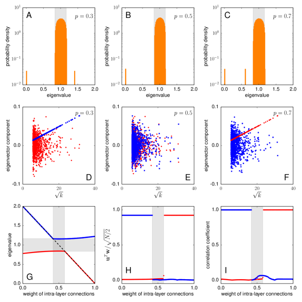
Figure 1: Abrupt transition in interconnected networks. Spectral analysis of the normalized laplacian $\mathcal{L}$ of an interconnected network composed of two network layers of size $N=1024$. The degree sequence is composed of integers extracted from a power-law probability distribution with exponent $\gamma=2.5$ defined on the support $[32,N]$. Intra- and inter-layer degree sequences are perfectly aligned so that the correlation term reads $\xi=\sum_{k^{in},k^{out}}k^{in}\,k^{out}\;P(k^{in},k^{out})=\langle k^{2}\rangle$. As the weight of the intra-layer layer connections $p$ varies, the system explores different regimes clearly visible from the spectrum of $\mathcal{L}$. A For $p=0.3$, only the largest eigenvalue $\nu_{2N}$ is well separated from the rest of the spectrum. The system is said to be in the “bipartite” regime ($\mathcal{B}$-phase). B For $p=0.5$, there are no detached eigenvalues. The system is in the “indistinguishable” regime ($\mathcal{I}$-phase). C For $p=0.7$, the second smallest eigenvalue $\nu_{2}$ is well separated for the rest of the spectrum. The system is in the “decoupled” regime ($\mathcal{D}$-phase). D In the $\mathcal{B}$-phase, the components of largest eigenvector $\mathbf{w}_{2N}$ corresponding to a single network layer (blue squares) are linearly correlated with the square root of the respective node degrees $\sqrt{k}$, while those of the second smallest eigenvector $\mathbf{w}_{2}$ (red circles) are not. E In the $\mathcal{I}$-phase, there is no correlation between the components of $\mathbf{w}_{2N}$ ($\mathbf{w}_{2}$) and $\sqrt{k}$. F In the $\mathcal{D}$-phase, the components of second smallest eigenvector $\mathbf{w}_{2}$ are linearly correlated with $\sqrt{k}$, while the components of $\mathbf{w}_{2N}$ are not. G The transition points $p_{c}^{-}\simeq 0.42$ and $p_{c}^{+}\simeq 0.58$ (delimiting the vertical gray area) between the different regimes correspond to the points in which our prediction [Eq. (5), black dashed line] enters the continuous band of the spectrum [Eq. (4), horizontal gray area]. Red circles refer to $\nu_{2}$, while blue squares refer to $\nu_{2N}$. H The sums of the components of $\mathbf{w}_{2}$ (red circles) and $\mathbf{w}_{2N}$ (blue squares) corresponding to nodes of a single network layer can be used as a order parameter to monitor the transition between the different regimes ($\mathbf{u}$ is the vector whose components are all equal to one). I As noted above, in the $\mathcal{D}$-phase ($\mathcal{B}$-phase), the components of $\mathbf{w}_{2}$ ($\mathbf{w}_{2N}$) are perfectly correlated with the square root of the node degrees.

Let us consider a symmetric and weighted interconnected network formed by two interconnected layers of identical size $N$ whose adjacency matrix $G$ is written in the block form

$$G=p\,G_{in}+(1-p)\,G_{out}=p\left(\begin{array}[]{cc}A&\emptyset\\ \emptyset&B\end{array}\right)+(1-p)\left(\begin{array}[]{cc}\emptyset&C\\ C^{T}&\emptyset\end{array}\right)\;.$$ (1)

$A$, $B$ and $C$ are $N\times N$ square matrices. $A$ and $B$ are symmetric matrices, while $C$ is not necessarily symmetric. According to Eq. (1), the adjacency matrix $G$ is a convex linear combination of the intra- and inter-layer adjacency matrices $G_{in}$ and $G_{out}$, and the parameter $p\in[0,1]$ serves to continuously tune the entire network from a bipartite graph ($p=0$) to a perfectly decoupled networked system ($p=1$). The normalized graph laplacian associated with the adjacency matrix of Eq. (1) is defined as

$$\mathcal{L}=\mathbbm{1}-D^{-1/2}GD^{-1/2}\;.$$ (2)

In the definition of $\mathcal{L}$, $\mathbbm{1}$ is the identity matrix, and $D^{-1/2}$ is a diagonal matrix whose diagonal elements are equal to the inverse of the square root of the node strengths Chung (1996). Since $G$ is symmetric, all the eigenvalues of $\mathcal{L}$ are real numbers in the range $[0,2]$. For simplicity, we sort them in ascending order such that $0=\nu_{1}\leq\nu_{2}\leq\cdots\nu_{2N}\leq 2$, and we indicate with $\mathbf{w}_{i}$ the eigenvector associated to $\nu_{i}$. The smallest eigenpair $(\nu_{1},\mathbf{w}_{1})$ is generally said to be “trivial” because it depends only on the strength sequence of the graph. We always have $\nu_{1}=0$ and $\mathbf{w}_{1}^{T}=1/\sqrt{2N\langle s\rangle}\left(\sqrt{s_{1}},\ldots,\sqrt{s_{2N}}\right)$, with $\langle s\rangle$ first moment of the strength distribution, and $s_{i}$ strength of the node $i$. When translated into the language of random walk dynamics, $\mathbf{w}_{1}$ tells us that, independently of the initial conditions and the topology of the network, the stationary probability to find the random walker on a given node is linearly proportional to its strength. The other two external eigenvalues $\nu_{2}$ and $\nu_{2N}$, and their associated eigenvectors $\mathbf{w}_{2}$ and $\mathbf{w}_{2N}$, are much more meaningful from the structural and dynamical points of view. $\nu_{2}$ is always strictly larger than zero in graphs composed of a single connected component. The associated eigenvector $\mathbf{w}_{2}$ is typically used in graph clustering to determine the bisection corresponding to the minimum of the normalized cut of the graph Jianbo and Jitendra (1997). In terms of random walk dynamics, such eigenvector is also very meaningful because the signs of its components define the so-called almost invariant sets of the graph Schwartz and Billings (2006); Rosvall and Bergstrom (2008). In essence, a random walker spends most its time moving among nodes whose correspondent components in $\mathbf{w}_{2}$ have the same sign, and less frequently jumps between nodes whose correspondent components in $\mathbf{w}_{2}$ have different signs. The largest eigenvalue $\nu_{2N}=2$ only if the graph is bipartite, while $\nu_{2N}<2$ in all other cases, and the components of $\mathbf{w}_{2N}$ identify the bipartite components of the graph. A random walker typically jumps between pairs of nodes that correspond to components of $\mathbf{w}_{2N}$ with different signs.

To understand the spectral properties of $\mathcal{L}$, we restrict our attention to the case of random network models generated according to the following procedure. Intra- and inter-layer degrees of both network layers $A$ and $B$ are respectively given by the same identical intra- and inter-layer degree sequences $k_{in}=\left\{k_{1}^{in},k_{2}^{in},\ldots,k_{N}^{in}\right\}$ and $k_{out}=\left\{k_{1}^{out},k_{2}^{out},\ldots,k_{N}^{in}\right\}$. The numbers appearing in the two degree sequences are also identical except for their order of appearance. The intra- and inter-layer degree distributions are thus identical $P(k^{in})=P(k^{out})=P(k)$, while the alignment between the two sequences regulates the joint probability distribution $P(k^{in},k^{out})$ of both network layers. In the construction of the network, internal and external connections are randomly placed with the only constraints of preserving the a priori provided degree sequences and generating network layers composed of a single connected component, so that $\nu_{2}>0$ and $\nu_{2N}<2$ for every $p\in(0,1)$. It is worth to briefly discuss the meaning, limitations and justifications of the previous assumptions. The fact that intra- and inter-layer connections are randomly placed allows us to say that no substructure is present in layers $A$ and $B$. Although this is not a good assumption for real networks that instead often exhibit modular structure at single layer level Fortunato (2010), it is a necessary assumption to concentrate our attention only on the effect of the layer structure on the spectrum of $\mathcal{L}$. The fact that the intra- and inter-layer degree distributions are identical, and both network layers have the same degree distribution and joint probability function $P(k^{in},k^{out})$ are also non realistic assumptions. In real world interconnected networks, in fact, one should expect the various distributions to be different. Although our general solution requires a much weaker assumption (see SI), here we decided to impose these constraints for illustrative purposes. The scenario is in fact already so much rich that having an additional symmetry in the system makes easier the explanation of the various behaviors that the system can exhibits.

If we think in terms of random walk dynamics, our network models are symmetric in two ways. First, the stationary probability to find the random walker in one of the two layers is equal to $1/2$. Second, they introduce a symmetry around the point $p=1/2$ for the various regimes in which the system can be tuned by varying $p$. Intuitively, we expect the following: (i) For $p<1/2$, the network should be in a “bipartite” regime ($\mathcal{B}$-phase) with the random walker moving more often from one layer to the other, and less frequently diffusing in the same layer; (ii) For $p>1/2$, the network should be in a “decoupled” regime ($\mathcal{D}$-phase) with the random walker more likely diffusing between nodes of the same layer, and less likely jumping between layers; (iii) For $p\simeq 1/2$, the network should be in a “indistinguishable” regime ($\mathcal{I}$-phase), with the random walker moving between and among layers with equal probability. Please note that, in the $\mathcal{I}$-phase, the system is topologically and dynamically identical to a single-layer network, thus in a potentially safe state. On contrary, when layers are structurally and dynamically distinguishable (i.e., $\mathcal{B}$- and $\mathcal{D}$-phases), then the network behaves as an interconnected network, and, as such, is exposed to potentially catastrophic failures or anomalous dynamical behavior. Intuitively, one should expect that the network is driven in a continuous way among the different phases as $p$ is varied. In reality, the scenario is much more complicated and appealing.

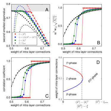
Figure 2: Phase diagram. We consider interconnected networks composed of two layers of size $N=8192$ with intra- and inter-layer degrees obeying a Poisson distribution with average $\langle k\rangle=32$. A Second smallest eigenvalue $\nu_{2}$ as a function of the weight of the intra-layer connections $p$. For values of the correlation term $\xi$ in the range $[\langle k\rangle^{2},\langle k^{2}\rangle]$, the results of numerical computations (symbols) are in very good agreement with our analytic predictions (dashed lines). The critical point $p_{c}^{+}$ is determined as the point for which the dashed lines enter the spectral band (gray area). For $\xi=\xi_{min}$, our predictions fail to correctly describe how $\nu_{2}$ changes as a function of $p$. B As in Fig. 1, we monitor the transition between the $\mathcal{D}$- and the $\mathcal{I}$-phase, by looking at the order parameter $\mathbf{u}^{T}\mathbf{w}_{2}/\sqrt{N/2}$. As $\xi$ decreases, the change of the order parameter becomes smoother, and the value of the critical point gets closer to $p=0.5$. For $\xi\in[\langle k\rangle^{2},\langle k^{2}\rangle]$, the order parameter goes to zero if $p<p_{c}^{+}$. For $\xi=\xi_{min}$ instead, the order parameter is larger than zero even for $p=0.5$. C The same behavior described for the order parameter is visible if we monitor the transition through the linear correlation coefficient between the eigenvector components and the r.h.s of Eq. (6). D Phase diagram representing the expected behavior of the system in the thermodynamic limit. The red line stands for the critical value $p_{c}^{+}$, while the blue line represents $p_{c}^{-}$ [Eq. (9)]. These critical values are plotted as functions of the quantity $\langle k^{2}\rangle-\xi$, ranging between zero and $\langle k^{2}\rangle-\xi_{min}$. As a reference, the dashed line represents the point at which $\xi=\langle k^{2}\rangle$. Although the curves corresponding to $p_{c}^{+}$ and $p_{c}^{-}$ do not intersect, for values of the correlation term $\xi$ sufficiently low, their analytic continuations suggest the disappearance of the $\mathcal{I}$-phase, and the appearance of a supercritical regime where both the bipartite and the decoupled phases are present (i.e., $\mathcal{BD}$-phase).

Let us first focus on the exactly solvable case in which the intra- and inter-layer degree sequences of both layers are ordered in the same way ($k^{in}_{i}=k^{out}_{i}=k_{i}$, for all nodes $i$). Please note that in this case the node strengths equal the node degrees, and thus they do not change with $p$ [$s_{i}=pk_{i}^{in}+(1-p)k_{i}^{out}=k_{i}$, for all nodes $i$]. In addition to the trivial eigenpair, $\mathcal{L}$ has always another eigenpair $(\nu^{*},\mathbf{w}^{*})$ given by

$$\nu^{*}=2(1-p)\qquad\textrm{ and }\qquad w^{*}_{i}=c_{i}\,\sqrt{k_{i}}\quad,\,\forall\,i=1,\ldots,2N\;,$$ (3)

where $c_{i}=c$, for $i=1,\ldots,N$, and $c_{i}=-c$, for $i=N+1,\ldots,2N$, and $c=1/\sqrt{2N\langle k\rangle}$ with $\langle k\rangle$ first moment of the degree distribution (see SI). Eq. (3) tells us that the eigenvector $\mathbf{w}^{*}$ is able to perfectly reflect the layer structure of the system. Such eigenvector is associated to an eigenvalue that spans the entire range $[0,2]$, and therefore must intersect all the other eigenvalues of $\mathcal{L}$. At each point of intersection, two orthogonal eigenvectors correspond to the same eigenvalue, and thus, in physical terms, each point of intersection corresponds to a degenerate energy level. Such phenomenology is typical of discontinuous phase transitions Blundell and Blundell (2006). Please note that this happens in networks of any size, and for any degree distribution. The changes between the various phases that we described above are of the same nature: as $p$ is increased, the system moves discontinuously from the $\mathcal{B}$-phase to the $\mathcal{I}$-phase, and from the $\mathcal{I}$-phase to the $\mathcal{D}$-phase. The $\mathcal{B}$-phase can be identified as the regime in which $\nu^{*}$ corresponds to the largest eigenvalue of $\mathcal{L}$. Similarly, the $\mathcal{D}$-phase can be determined as the regime in which $\nu^{*}$ represents the second smallest eigenvalue of $\mathcal{L}$. Finally in the $\mathcal{I}$-phase, $\nu^{*}$ is inside the spectrum of $\mathcal{L}$. The values of $p$ for which phase transitions occur can be approximately estimated with the following argument. Numerical computations of the spectrum of $\mathcal{L}$ show that, whereas the eigenvalue $\nu^{*}$ is rapidly changing as a function of $p$, all other eigenvalues vary much more slowly (see upper panels of Fig. 1). The graph obtained for $p=1/2$ can be thus be used as a representative for this almost constant behavior. We can then approximate, thanks to the prediction of Chung et al. Chung et al. (2003), the expected spectral radius of the normalized laplacian of a random graph with prescribed degree distribution as

$$\max_{i>1}\left|1-\nu_{i}\right|\simeq\frac{2}{\sqrt{2\langle k\rangle}}\;.$$ (4)

Eq. (4) generally provides very good estimates for the spectral radius of $\mathcal{L}$ for random networks with poissonian and power-law degree distributions. By comparing $\nu^{*}$ to the r.h.s. of Eq. (4), we finally find that the two transition points are

$$p_{c}^{+,-}\simeq\frac{1}{2}\pm\frac{1}{\sqrt{2\langle k\rangle}}\;.$$ (5)

In Eq. (5), the solution with the minus sign corresponds to critical point of the transition between the $\mathcal{B}$- and $\mathcal{I}$-phases, while the solution with the plus sign corresponds to threshold between the $\mathcal{I}$- and $\mathcal{D}$-phases. As expected, such predictions are in very good agreement with the results of numerical experiments (see Fig. 1).

Next, we relax the former assumption about perfectly aligned degree sequences, and we let $k_{out}$ correspond to a slightly modified permutation of the sequence $k_{in}$. Unfortunately, our theory works only for Poisson degree distributions, but the results we obtain allows us to understand also the qualitative behavior of networks with power-law degree distributions. If degrees are random variates extracted from a Poisson distribution, we are able to numerically show that the $i$-th component of the second smallest (only in the $\mathcal{D}$-phase) or the largest eigenvector (only in the $\mathcal{B}$-phase) $\mathbf{w}^{*}$ obeys the relation

$$w^{*}_{i}\;\simeq c_{i}\;\frac{p\,k_{i}^{in}-(1-p)\,k_{i}^{out}}{\sqrt{p\,k_{i}^{in}+(1-p)\,k_{i}^{out}}}\;,$$ (6)

where $c_{i}=c$, for $i=1,\ldots,N$, and $c_{i}=-c$, for $i=N+1,\ldots,2N$, and $c$ is a proper normalization constant. This essentially means that the $i$-th component of the eigenvector $\mathbf{w}^{*}$ is proportional to the difference between the internal and external strengths divided by the square root of the total strength of node $i$ (Fig. S1). The validity of Eq. (6) is testified by the very high linear correlation coefficients that one can measure between the components of the eigenvectors (numerically computed), and the r.h.s. of Eq. (6). Using Eq. (6) as ansatz for the solution of the eigenvalue problem, we are able to determine that the eigenvalue of $\mathcal{L}$ associated to the eigenvector $\mathbf{w}^{*}$ of Eq. (6) is given by

$$\nu^{*}\simeq 1-\frac{\left(2p^{2}-2p+1\right)\,\langle k^{2}\rangle-2p(1-p)\,\xi}{\left(2p-1\right)\,\langle k^{2}\rangle}\;,$$ (7)

and thus by the ratio between a quadratic and a linear function of $p$. The function appearing at the denominator depends only on the second moment $\langle k^{2}\rangle$ of the degree distribution. The function appearing at the numerator, instead, depends on the second moment of the degree distribution, and the correlation between intra- and inter-layer degrees

$$\xi=\sum_{k^{in},k^{out}}k^{in}\,k^{out}\;P(k^{in},k^{out})\;.$$ (8)

By comparing Eq. (7) with the expected spectral radius of Eq. (4), we finally arrive to the prediction of the critical points

$$p_{c}^{+,-}\simeq\frac{1}{2}\left[1\pm\frac{\frac{2}{\sqrt{2\langle k\rangle}}\langle k^{2}\rangle+\sqrt{\xi^{2}+\langle k^{2}\rangle^{2}\left(\frac{2}{\langle k\rangle}-1\right)}}{2\left(\langle k^{2}\rangle+\xi\right)}\right]\;.$$ (9)

When the term inside the square root of Eq. (9) is larger than zero, we have an intersection between $\nu^{*}$ and the rest of spectrum of $\mathcal{L}$. This indicates the presence of an abrupt transition between the corresponding phases. Strictly speaking, these eigenvalues do not intersect in finite size random networks, as predicted by the Wigner-von Neumann noncrossing rule von Neumann and Wigner (1929); Lax (2007), however, the abrupt nature of the transition appears clear already for networks of moderately large size. When the term in the square root of Eq. (9) is equal to zero, the non trivial eigenvalue $\nu^{*}$ touches the rest of spectrum of $\mathcal{L}$ tangentially at $p_{c}$. In this case, the corresponding transition becomes continuous. The non existence of a real solution in Eq. (9) reveals instead the absence of a crossing between $\nu^{*}$ and the rest of the spectrum even in infinite size networks, and thus is the sign of a dramatic change in the behavior of the system.

Eqs. (7) and (9) show that the the entire scenario is characterized by two main factors. On one end, the degree distribution, with its first two moments, play a fundamental role for the determination of the various phases. On the other hand, the degree distribution alone is not able to explain the behavior of the system. At parity of moments in fact, the features of the system can be still drastically changed by the correlation term defined in Eq. (8). To better understand how the various possibilities are regulated by the interplay between the correlation term $\xi$ and the moments of the degree distribution, we vary the correlation term by regulating the alignment between the intra- and inter-layer degree sequences $k_{in}$ and $k_{out}$. If the order of the sequences $k_{in}$ and $k_{out}$ is identical, $\xi=\langle k^{2}\rangle$, and Eqs. (7) and (9) correctly reduce to Eqs. (3) and (5), respectively. If from this initial alignment we randomly shuffle a selected portion of pairs of entries in the inter-layer degree sequence $k_{out}$, we decrease the value of $\xi$. In particular, if we randomly mix all entries, then $k_{out}$ corresponds to a random permutation of $k_{in}$ and the correlation term reads $\xi=\langle k\rangle^{2}$. Finally, if the entries of $k_{in}$ are ordered in ascending (descending) order, while those of $k_{out}$ are sorted in descending (ascending) order, the correlation term reaches the minimum value $\xi_{min}$ Darćzy (1973). When $\xi$ is in the range $[\langle k\rangle^{2},\langle k^{2}\rangle]$, the term in the square root of Eq. (9) is strictly larger than zero: all regimes exist, and the corresponding phase transitions are discontinuous (see Fig. 2). At the same time, the phase diagram suggests that a further decrement of $\xi$ leads to a drastic mutation in the features of the system. For lower values of $\xi$, the analytic continuation of our predictions tell us: (i) phase transitions change their nature and become continuous; (ii) the $\mathcal{I}$-phase is not longer present, and leaves space to an hybrid $\mathcal{BD}$-phase where the system is simultaneously in both the bipartite and decoupled regimes. The presence of this hybrid phase appears evident by looking at the spectral properties of the normalized laplacian even of finite size systems: for $\xi=\xi_{min}$ and $p=0.5$, the order parameters associated to the $\mathcal{B}$- and $\mathcal{D}$-phases are in fact simultaneously larger than zero (see Figs. 2 and S2).

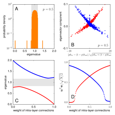
Figure 3: Supercritical regime. Spectral analysis of the normalized laplacian $\mathcal{L}$ for an interconnected network with degree sequence identical to the one analyzed in Fig. 1. In this case, however, intra- and inter-layer degree sequences are aligned in such a way that the correlation term is $\xi\simeq 1/2(\langle k^{2}\rangle+\langle k\rangle^{2})$. A For $p=0.5$, the system is in the $\mathcal{BD}$-phase, where both the eigenvalues $\nu_{2}$ and $\nu_{2N}$ are well separated from the other eigenvalues of $\mathcal{L}$. B The components of both eigenvectors $\mathbf{w}_{2}$ and $\mathbf{w}_{2N}$ are correlated with the r.h.s. of Eq. (6). C The eigenvalues $\nu_{2}$ (red circles) and $\nu_{2N}$ (blue squares) touch the continuous band tangentially. D The order parameter clearly shows the presence of supercritical regime, where both the $\mathcal{B}$- and $\mathcal{D}$-phases are simultaneously present, for a wide range of values of $p$. Only for very low (large) values of $p$, the system is in the pure $\mathcal{B}$-phase ($\mathcal{D}$-phase).

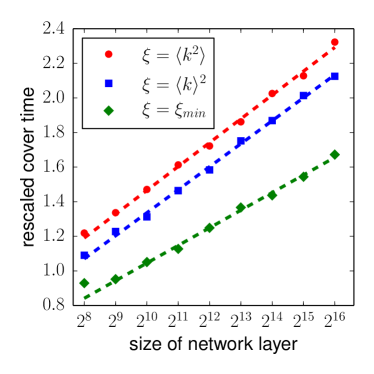
Figure S4: Cover time $T_{cover}$ of a random walker moving in an interconnected network composed of two layers of $N$ nodes. The degrees are extracted from a power-law distribution with exponent $\gamma=2.5$ defined on the support $[5,N]$. Cover time is divided by the sum of the strengths of all nodes in the network. The weight $p$ of intra-layer connections is set equal to $0.5$. Each point represents the average value of the normalized cover time obtained in at least $100$ realizations of the network models. The dashed lines stand for fits with the function $T_{cover}=a+b\log{N}$. We measure $b=0.20$ (red), $b=0.19$ (blue) and $b=0.15$ (green).

The previous effect is amplified when we consider networks whose degrees obey a power-law degree distribution $P(k)\sim k^{-\gamma}$, with $\gamma<3$. Differently from the case of poissonian networks in fact, the correlation term $\xi$ has a much larger range of variability. Although the ansatz of Eq. (6) breaks down for scale-free networks, and thus the entire analytic approach is not working, Eq. (9) still tells us what we should expect to see: unless the correlation term $\xi$ is very close to its maximal value $\langle k^{2}\rangle$, the term in the square root is negative; this means that the $\mathcal{BD}$-phase is reached already for little variations from the perfect alignment between the intra- and inter-layer sequences $k_{in}$ and $k_{out}$. This is indeed verified in our numerical experiments as shown in Figs. 3 and S3. For $p=0.5$, the presence of the hybrid $\mathcal{BD}$-phase is testified by the fact that the eigenvalues $\nu_{2}$ and $\nu_{2N}$ are simultaneously well separated from the other eigenvalues of $\mathcal{L}$, and the associated eigenvectors $\mathbf{w}_{2}$ and $\mathbf{w}_{2N}$ have components that are very well correlated with the r.h.s of Eq. (6). The mixing between the two degree sequences causes a mismatch between intra- and inter-layer hubs which do not correspond to the same nodes as in the case of perfectly aligned degree sequences. From the structural point of view, the total disappearance of the so-called indistinguishable phase can be interpreted as the absence of a buffer of structural safety. Scale-free networks seem therefore to be constantly at risks of potentially catastrophic failures. There are, however, also dramatic dynamical consequences. While for high values of $\xi$ there is a neat distinction between the $\mathcal{B}$- and $\mathcal{D}$-phases and a random walker moves in the network performing either intra- or inter-layer diffusion, in the $\mathcal{BD}$-phase instead both motions happen simultaneously (Fig. 4). Such ability makes the walker faster in the exploration of the entire system (Fig. S4).

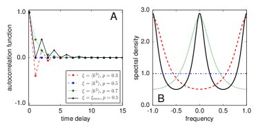
Figure 4: Random walk dynamics. We consider two interconnected networks composed of $N=8192$ nodes. Degrees are extracted from a power-law distribution with exponent $\gamma=2.5$ defined on the support $[32,N]$. We monitor the trajectory of a random walker moving on these systems for different values of the correlation term $\xi$ and different values of the weight of the intra-layer connections $p$. A Autocorrelation function $R(\tau)=\langle x(t)x(t+\tau)\rangle$ as a function of the time delay $\tau$. In the definition of $R(\tau)$, $x(t)=+1$ if the random walker is on layer $A$ at time $t$, and $x(t)=-1$, otherwise. B Spectral density $S(\omega)$ of the autocorrelation functions of panel A. Intra-layer movements are characterized by the presence of a peak of $S(\omega)$ at $\omega=0$, while inter-layer jumps are emphasized by the presence of peaks at $\omega=\pm 1$.

To summarize, the spectral properties of the normalized laplacian of random interconnected networks show that these systems face a scenario that is much richer than the one valid for isolated networks. Depending on the combination of basic structural properties – degree distribution, degree correlation, and strength difference between intra- and inter-layer connections – topological and dynamical phase transitions associated to the spectrum of the normalized laplacian can be either discontinuous or continuous, and different regimes can disappear or even coexist. This allows us, somehow, to divide the space of structural parameters in regions where the “classical” theory of isolated network holds, and those in which interdependent networks behave in anomalous manner. As a final remark, we would like to stress an appealing analogy between our findings and the typical thermodynamic behavior of any substance, e.g., water, carbon dioxide and methane. In normal conditions, a substance changes its phase from liquid to gas in a discontinuous manner. However, above its critical temperature and pressure, the substance ceases to exhibit distinct liquid- or gas-like state, and it becomes a so-called supercritical fluid McHugh and Krukonis (1986). Since their properties can be fine-tuned, supercritical fluids have many industrial and scientific applications. We believe that the possibility to drive interconnected networks to supercritical regimes could also be used in a fruitful way to better design and control real world networked systems.

Supplementary Information

Preliminary definitions

We consider a symmetric and weighted interconnected network formed by two network layers of identical size $N$. The adjacency matrix $G$ of the entire network can be written in the block form

$$G=\left(\begin{array}[]{cc}A&C\\ C^{T}&B\end{array}\right)\;.$$ (S1)

$A$, $B$ and $C$ are $N\times N$ square symmetric and weighted matrices. $A$ and $B$ represent the weighted adjacency matrices of the two network layers and thus contain information only about intra-layer connections, the matrix $C$ lists instead all the inter-layer connections among nodes of different layers. When comparing Eq. (S1) with Eq. (1) of the main text, please consider that the factors $p$ and $1-p$ have been implicitly included in the definition of Eq. (S1). We can reduce Eq. (S1) Eq. (1) of the main text if we perform the substitutions $A\to pA$, $B\to pB$, $C\to(1-p)C$ and $C^{T}\to(1-p)C^{T}$.

For simplicity of notation, let us define the in-strength vector $\left|s^{in}_{A}\right>=A\left|1\right>$ of layer $A$ as the vector whose $i$-th component is given by the sum the weights of all edges that connect node $i\in A$ to other nodes of network layer $A$. Similar definitions apply also to the out-strength vector $\left|s^{out}_{A}\right>=C\left|1\right>$, and to the analogues for layer $B$, that are $\left|s^{in}_{B}\right>=B\left|1\right>$ and $\left|s^{out}_{B}\right>=C^{T}\left|1\right>$. Please note that we are making use of the standard bra-ket notation for vectors, and we have indicated with $\left|1\right>$ the vector whose components are all equal to one. Clearly, the strength vectors of the network layers $A$ and $B$ are simply given by $\left|s_{A}\right>=\left|s^{in}_{A}\right>+\left|s^{out}_{A}\right>$ and $\left|s_{B}\right>=\left|s^{in}_{B}\right>+\left|s^{out}_{B}\right>$, respectively, while the components of the vectors $\left|\Delta s_{A}\right>=\left|s^{in}_{A}\right>-\left|s^{out}_{A}\right>$ and $\left|\Delta s_{B}\right>=\left|s^{in}_{B}\right>-\left|s^{out}_{B}\right>$ quantify the difference between intra- and inter-layer connections of the various nodes. Please note that all the former vectors are composed of $N$ entries.

Normalized Laplacian

Consider now the normalized laplacian matrix derived from the adjacency matrix of Eq. (S1), given by

$$\mathcal{L}=\mathbbm{1}-D^{-1/2}GD^{-1/2}\;,$$ (S2)

where

$$D=\left(\begin{array}[]{cc}D_{A}&\emptyset\\ \emptyset&D_{B}\end{array}\right)\;.$$ (S3)

$D_{A}$ and $D_{B}$ are two diagonal matrices such that the $i$-th diagonal elements are $\left(D_{A}\right)_{i,i}=\left(\left|s_{A}\right>\right)_{i}$ (i.e., the $i$-th component of the vector $\left|s_{A}\right>$) and $\left(D_{B}\right)_{i,i}=\left(\left|s_{B}\right>\right)_{i}$ (i.e., the $i$-th component of the vector $\left|s_{B}\right>$).

In order to solve in a simpler way the eigenvalue problem

$$\mathcal{L}\left|w\right>=\nu\left|w\right>\,$$

it is better to consider the matrix

$$D^{-1/2}\mathcal{L}D^{1/2}=\mathbbm{1}-D^{-1}G\;,$$ (S4)

where $\mathbbm{1}$ is the identity matrix, and $D^{-1}G$ is the so-called random walk matrix. Since $\mathcal{L}$ and $\mathbbm{1}-D^{-1}G$ are related by a similarity transformation, they share the same spectrum. The right eigenvector $\left|w\right>$ of $\mathcal{L}$ is related to the left eigenvector of $\left|u\right>$ of $\mathbbm{1}-D^{-1}G$ by

$$\left|w\right>=D^{-1/2}\left|u\right>\;,$$

while the right eigenvector $\left|w\right>$ of $\mathcal{L}$ is related to the right eigenvector of $\left|v\right>$ of $\mathbbm{1}-D^{-1}G$ by

$$\left|w\right>=D^{1/2}\left|v\right>\;,$$

and consequently the left eigenvector $\left|u\right>$ of $\mathbbm{1}-D^{-1}G$ and the right eigenvector of $\left|v\right>$ of $\mathbbm{1}-D^{-1}G$ are related by

$$\left|v\right>=D^{-1}\left|u\right>\;.$$

For our purposes, it is even more convenient to rewrite the eigenvalue problem as follows

$$\mathbbm{1}\left|v\right>-D^{-1}G\left|v\right>=\nu\left|v\right>\;,$$

$$D^{-1}G\left|v\right>=(1-\nu)\left|v\right>$$

and

$$G\left|v\right>=(1-\nu)D\left|v\right>\;.$$

Please note that previous equation has one trivial solution given by given by $1-\nu=0$ and $\left|v\right>=\left|1\right>$, thus any other eigenvector with different eigenvalue must be orthogonal to $\left|1\right>$.

If we write the eigenvector $\left|v\right>=\left|v_{A},v_{B}\right>$ as the composition of two vectors $\left|v_{A}\right>$ and $\left|v_{B}\right>$ with $N$ entries each corresponding to the nodes of layers $A$ and $B$, respectively, the previous equation is equivalent to the coupled equations

$$\begin{array}[]{l}A\left|v_{A}\right>+C\left|v_{B}\right>=\left(1-\nu\right)D_{A}\left|v_{A}\right>\\ B\left|v_{B}\right>+C^{T}\left|v_{A}\right>=\left(1-\nu\right)D_{B}\left|v_{B}\right>\end{array}\;.$$ (S5)

If we multiply these equations for $\left<1\right|$, we have

$$\begin{array}[]{l}\left<1\right|A\left|v_{A}\right>+\left<1\right|C\left|v_{B}\right>=\left(1-\nu\right)\left<1\right|D_{A}\left|v_{A}\right>\\ \left<1\right|B\left|v_{B}\right>+\left<1\right|C^{T}\left|v_{A}\right>=\left(1-\nu\right)\left<1\right|D_{B}\left|v_{B}\right>\end{array}$$

$$\begin{array}[]{l}\left<s_{A}^{in}|v_{A}\right>+\left<s_{B}^{out}|v_{B}\right>=\left(1-\nu\right)\left<s_{A}|v_{A}\right>\\ \left<s_{B}^{in}|v_{B}\right>+\left<s_{A}^{out}|v_{A}\right>=\left(1-\nu\right)\left<s_{B}|v_{B}\right>\end{array}$$

If we take their difference, we have

$$\left(1-\nu\right)\left(\left<s_{A}|v_{A}\right>-\left<s_{B}|v_{B}\right>\right)=\left<\Delta s_{A}|v_{A}\right>-\left<\Delta s_{B}|v_{B}\right>$$

if we finally suppose that $\left<s_{A}|v_{A}\right>-\left<s_{B}|v_{B}\right>\neq 0$, this becomes

$$\nu=1-\frac{\left<\Delta s_{A}|v_{A}\right>-\left<\Delta s_{B}|v_{B}\right>}{\left<s_{A}|v_{A}\right>-\left<s_{B}|v_{B}\right>}\;.$$

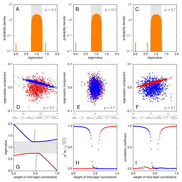
Figure S1: Spectral analysis of the normalized laplacian $\mathcal{L}$ of an interconnected network composed of two network layers of size $N=1024$ with intra- and inter-layer degrees obeying a Poisson distribution with average degree $\langle k\rangle=32$. In- and out-degrees sequences are randomly mixed so that the correlation term reads $\xi=\langle k\rangle^{2}$. The description of the various panels is identical to the one of Fig. 1 of the main text. In panels D, E and F, the components of the eigenvectors $\mathbf{w}_{2}$ and $\mathbf{w}_{2N}$ are plotted as functions of the components of the vectors appearing on the r.h.s. of Eq. (S6). In Panel G, the dashed line stands for Eq. (S9).

Please note that the graphical closure of the graph imposes that

$$\left<1|s_{A}^{out}\right>=\left<1|s_{B}^{out}\right>\;.$$

When the internal strength of the both layers is comparable, i.e.,

$$\left<1|s_{A}^{in}\right>\simeq\left<1|s_{B}^{in}\right>\;,$$

then numerical computations of the spectrum of $\mathcal{L}$, such as those presented in Fig. S1, show that, the second smallest eigenvector (largest eigenvector) in the decoupled regime (bipartite regime) of the normalized laplacian is approximately given by

$$\begin{array}[]{l}\left|w_{A}\right>=n_{A}D_{A}^{-1/2}\left|\Delta s_{A}\right>\\ \left|w_{B}\right>=n_{B}D_{B}^{-1/2}\left|\Delta s_{B}\right>\end{array}\;,$$ (S6)

where $n_{A}$ and $n_{B}$ are normalization constants. This means that

$$\begin{array}[]{l}\left|v_{A}\right>=n_{A}\left|\Delta s_{A}\right>\\ \left|v_{B}\right>=n_{B}\left|\Delta s_{B}\right>\end{array}\;,$$ (S7)

Since $\left|v_{A},v_{B}\right>$ is orthogonal to $\left|1,1\right>$, we can write

$$n_{A}\left<1|\Delta s_{A}\right>+n_{B}\left<1|\Delta s_{B}\right>=0\;\leftrightarrow\;n_{A}=-n_{B}\frac{\left<1|\Delta s_{B}\right>}{\left<1|\Delta s_{A}\right>}$$

thus

$$\left<s_{A}|v_{A}\right>-\left<s_{B}|v_{B}\right>=-n_{B}\frac{\left<1|\Delta s_{B}\right>}{\left<1|\Delta s_{A}\right>}\left<s_{A}|\Delta s_{A}\right>-n_{B}\left<s_{B}|\Delta s_{B}\right>\;,$$

and

$$\begin{array}[]{l}\left<\Delta s_{A}|v_{A}\right>-\left<\Delta s_{B}|v_{B}\right>=\\ -n_{B}\frac{\left<1|\Delta s_{B}\right>}{\left<1|\Delta s_{A}\right>}\left<\Delta s_{A}|\Delta s_{A}\right>-n_{B}\left<\Delta s_{B}|\Delta s_{B}\right>\end{array}\;.$$

So in conclusion, the eigenvalue corresponding to this eigenvector is given by

$$\nu^{*}=1-\frac{\left<\Delta s_{A}|\Delta s_{A}\right>/\left<1|\Delta s_{A}\right>+\left<\Delta s_{B}|\Delta s_{B}\right>/\left<1|\Delta s_{B}\right>}{\left<s_{A}|\Delta s_{A}\right>/\left<1|\Delta s_{A}\right>+\left<s_{B}|\Delta s_{B}\right>/\left<1|\Delta s_{B}\right>}\;.$$ (S8)

Please note that

$$\left<\Delta s_{A}|\Delta s_{A}\right>=\sum_{i\in A}(s_{i}^{in}-s_{i}^{out})(s_{i}^{in}-s_{i}^{out})=\sum_{i\in A}(s_{i}^{in})^{2}+(s_{i}^{out})^{2}-2s_{i}^{in}s_{i}^{out}=N\left(m_{2,A}^{in}+m_{2,A}^{out}-2\xi_{A}\right)\;,$$

where $m_{2,A}^{in}$ is the second moment of the in-strength distribution of layer $A$, $m_{2,A}^{out}$ is the second moment of the out-strength distribution of layer $A$, and $\xi_{A}$ is the correlation between the in- and out-strength of nodes in layer $A$. Similarly, one can write

$$\left<\Delta s_{A}|s_{A}\right>=\sum_{i\in A}(s_{i}^{in}-s_{i}^{out})(s_{i}^{in}+s_{i}^{out})=\sum_{i\in A}(s_{i}^{in})^{2}-(s_{i}^{out})^{2}=N\left(m_{2,A}^{in}-m_{2,A}^{out}\right)\;,$$

$$\left<\Delta s_{A}|1\right>=\sum_{i\in A}(s_{i}^{in}-s_{i}^{out})=N\left(m_{1,A}^{in}-m_{1,A}^{out}\right)$$

and

$$\left<s_{A}|1\right>=\sum_{i\in A}(s_{i}^{in}+s_{i}^{out})=N\left(m_{1,A}^{in}+m_{1,A}^{out}\right)\;,$$

where $m_{1,A}^{in}$ and $m_{1,A}^{out}$ are the first moments of the in- and out-strength distribution, respectively. The same relations are also valid for layer $B$. Eq. (S8) can be thus rewritten as

$$\nu^{*}=1-\frac{(m_{2,A}^{in}+m_{2,A}^{out}-2\xi_{A})/(m_{1,A}^{in}-m_{1,A}^{out})+(m_{2,B}^{in}+m_{2,B}^{out}-2\xi_{B})/(m_{1,B}^{in}-m_{1,B}^{out})}{(m_{2,A}^{in}-m_{2,A}^{out})/(m_{1,A}^{in}-m_{1,A}^{out})+(m_{2,B}^{in}-m_{2,B}^{out})/(m_{1,B}^{in}-m_{1,B}^{out})}\;.$$

If we finally assume that both network layers have identical in- and out-strength distributions and identical correlations between in- and out-strengths, the former expression further simplifies to

$$\nu^{*}=1-\frac{m_{2}^{in}+m_{2}^{out}-2\xi}{m_{2}^{in}-m_{2}^{out}}\;.$$ (S9)

Please note that if we consider the adjacency matrix of Eq. 1 of the main text, we have to perform the following substitutions: $m_{2}^{in}\to p^{2}\langle k^{2}\rangle$, $m_{2}^{out}\to(1-p)^{2}\langle k^{2}\rangle$ and $\xi\to p(1-p)\xi$. We thus recover Eq. (7) of the main text.

Critical points

The critical points of the transitions are calculated as the values of $p$ for which Eq. (7) intersects the spectral band of Eq. (4) predicted by Chung et al. For $p\neq 1/2$, this leads to the equation

$$\frac{2p^{2}-2p+1}{2p-1}-2\frac{\xi}{\langle k^{2}\rangle}\frac{p(1-p)}{2p-1}=\pm\frac{2}{\sqrt{2\langle k\rangle}}\;,$$

from which

$$(2p^{2}-2p+1)\langle k^{2}\rangle-2p(1-p)\xi\mp\frac{2}{\sqrt{2\langle k\rangle}}\langle k^{2}\rangle(2p-1)=0$$

and finally

$$2p^{2}\left(\langle k^{2}\rangle+\xi\right)-2p\left[\langle k^{2}\rangle\left(1\pm\frac{2}{\sqrt{2\langle k\rangle}}\right)+\xi\right]+\langle k^{2}\rangle\left(1\pm\frac{2}{\sqrt{2\langle k\rangle}}\right)=0\;.$$

Such quadratic equation has discriminant given by

$$\Delta=4\left[\xi^{2}+\langle k^{2}\rangle^{2}\left(\frac{2}{\langle k\rangle}-1\right)\right]\;,$$ (S10)

and thus solution given by

$$p_{c}=\frac{1}{2}\left(1\pm\frac{\frac{2\langle k^{2}\rangle}{\sqrt{2\langle k\rangle}}\pm\sqrt{\xi^{2}+\langle k^{2}\rangle^{2}\left(\frac{2}{\langle k\rangle}-1\right)}}{2\left(\langle k^{2}\rangle+\xi\right)}\right)\;.$$

The solutions of this equations closer to $p=1/2$ are not not interesting for us because $\nu^{*}$ has already entered the spectrum at point. The effective critical points are thus given by Eq. (9) of the main text.

Positively/neutrally correlated network layers

A simple strategy to explore this regime of correlation is the following. We sort both the intra-layer and inter-layer degree sequences in ascending (descending) order, but we then shuffle, with probability $q$, each entry of the sequence with another randomly chosen entry. For $q=0$, the two sequences are identical and the correlation term reads $\xi=\langle k^{2}\rangle$. In this case, we say that network layers are positively correlated. For $q=1$, the out-degree sequence is effectively a random permutation of $k_{in}$, and the correlation term reads $\xi=\langle k\rangle^{2}$. We thus say that network layers are neutrally correlated. For general values of $q$, the correlation term obeys

$$\xi=(1-q)\langle k^{2}\rangle+q\langle k\rangle^{2}\;,$$

with $q\in[0,1]$.

The discriminant of Eq. (S10) becomes

$$\Delta=\left[(1-q)\langle k^{2}\rangle+q\langle k\rangle^{2}\right]^{2}+\langle k^{2}\rangle^{2}\left(\frac{2}{\langle k\rangle}-1\right)\;,$$

, and thus

$$\Delta=\left(1-2q+q^{2}+\frac{2}{\langle k\rangle}-1\right)\langle k^{2}\rangle^{2}+2q(1-q)\langle k^{2}\rangle\langle k\rangle^{2}+q^{2}\langle k\rangle^{4}\;,$$

$$\Delta=\left(-2q+q^{2}+\frac{2}{\langle k\rangle}\right)\langle k^{2}\rangle^{2}+2q(1-q)\langle k^{2}\rangle\langle k\rangle^{2}+q^{2}\langle k\rangle^{4}\;,$$

$$\Delta=q^{2}\left(\langle k^{2}\rangle^{2}-2\langle k^{2}\rangle\langle k\rangle^{2}+\langle k\rangle^{4}\right)-2q\langle k^{2}\rangle\left(\langle k^{2}\rangle-\langle k\rangle^{2}\right)+\frac{2}{\langle k\rangle}\langle k^{2}\rangle^{2}\;,$$

and

$$\Delta=q^{2}\left(\langle k^{2}\rangle-\langle k\rangle^{2}\right)^{2}-2q\langle k^{2}\rangle\left(\langle k^{2}\rangle-\langle k\rangle^{2}\right)+\frac{2}{\langle k\rangle}\langle k^{2}\rangle^{2}\;.$$

The value $q_{c}$ of $q$ for which $\Delta=0$ is therefore the solution of a quadratic equation in $q$. This is given by

$$q_{c}=\frac{1}{2\left(\langle k^{2}\rangle-\langle k\rangle^{2}\right)^{2}}\left[2\langle k^{2}\rangle\left(\langle k^{2}\rangle-\langle k\rangle^{2}\right)\pm\sqrt{4\langle k^{2}\rangle^{2}\left(\langle k^{2}\rangle-\langle k\rangle^{2}\right)^{2}-4\langle k^{2}\rangle^{2}\,2/\langle k\rangle\,\left(\langle k^{2}\rangle-\langle k\rangle^{2}\right)^{2}}\right]\;,$$

from which we finally find

$$q_{c}=\frac{\langle k^{2}\rangle}{\langle k^{2}\rangle-\langle k\rangle^{2}}\left[\;1\pm\sqrt{1-\frac{2}{\langle k\rangle}}\;\right]\;.$$

Please note that $\frac{\langle k^{2}\rangle}{\langle k^{2}\rangle-\langle k\rangle^{2}}\geq 1$, thus the only solution that is potentially smaller or equal to one

$$q_{c}=\frac{\langle k^{2}\rangle}{\langle k^{2}\rangle-\langle k\rangle^{2}}\left[\;1-\sqrt{1-\frac{2}{\langle k\rangle}}\;\right]\;.$$

For poissonian graphs, the former expression shows that $q_{c}>1$. Thus for any value of $q\in[0,1]$ $\Delta>0$. For scale-free graphs with degree exponent $\gamma<3$ instead, $\frac{\langle k^{2}\rangle}{\langle k^{2}\rangle-\langle k\rangle^{2}}\simeq 1$, and $q_{c}\leq 1$.

Negatively/neutrally correlated network layers

To explore this regime of correlation, we sort both the intra-layer in ascending (descending) order and inter-layer degree sequences in descending (ascending) order, but we then shuffle, with probability $t$, each entry of the sequence with another randomly chosen entry. For $t=0$, the correlation term reads $\xi=\xi_{min}$ and the layers are negatively correlated. For $t=1$, the out-degree sequence is effectively a random permutation of $k_{in}$, and the correlation term reads $\xi=\langle k\rangle^{2}$. Network layers are neutrally correlated. For general values of $t$, the correlation term obeys

$$\xi=(1-t)\xi_{min}+t\langle k\rangle^{2}\;,$$

with $t\in[0,1]$. The discriminant is therefore

$$\Delta=\left[(1-t)\xi_{min}+t\langle k\rangle^{2}\right]^{2}+\langle k^{2}\rangle^{2}\left(\frac{2}{\langle k\rangle}-1\right)\;.$$

This becomes

$$\Delta=t^{2}\left(\xi_{min}-\langle k\rangle^{2}\right)^{2}-2t\xi_{min}\left(\xi_{min}-\langle k\rangle^{2}\right)+\xi_{min}^{2}+\langle k^{2}\rangle^{2}\left(\frac{2}{\langle k\rangle}-1\right)\;.$$

Thus the critical value of $t$ is given by

$$t_{c}=\frac{1}{\xi_{min}-\langle k\rangle^{2}}\left[\;\xi_{min}\pm\langle k^{2}\rangle\sqrt{1-\frac{2}{\langle k\rangle}}\;\right]\;.$$

The solution with the plus sign is always negative, thus

$$t_{c}=\frac{\langle k^{2}\rangle\sqrt{1-\frac{2}{\langle k\rangle}}-\xi_{min}}{\langle k\rangle^{2}-\xi_{min}}\;.$$

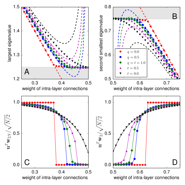
Figure S2: We consider interconnected networks composed of two network layers of size $N=8192$ with intra- and inter-layer degrees obeying a Poisson distribution with average degree $\langle k\rangle=32$. As explained in the text, the continuous parameters $q$ and $t$ are used to control the alignment between the entries of the two degree sequences sequences, so that the correlation term reads $\xi=(1-q)\langle k^{2}\rangle+q\langle k\rangle^{2}$ or $\xi=(1-t)\xi_{min}+t\langle k\rangle^{2}$. A For any value of $q$, the largest eigenvalue $\nu_{2N}$ intersects the continuous band (gray area). The corresponding transition, in the thermodynamic limit, is expected to be discontinuous. The results of numerical computations (symbols) are in very good agreement with our analytic predictions (dashed lines). For $t<1$, our predictions fail to correctly describe how $\nu_{2N}$ changes as a function of the weight of the intra-layer connections. B Same as for panel A, but for the second smallest eigenvalue $\nu_{2}$. C Sum of the components of $\mathbf{w}_{2N}$ corresponding to nodes of a single layer. D Same as for panel C, but for the second smallest eigenvector $\mathbf{w}_{2}$.

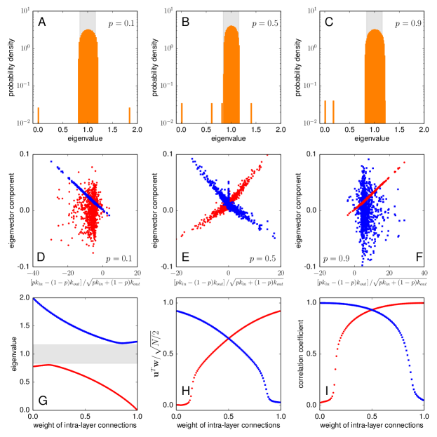
Figure S3: Spectral analysis of the normalized laplacian $\mathcal{L}$ the scale-free interconnected network analyzed in Fig. 3 of the main text. A When the weight of the intra-layer connections $p$ is sufficiently low, the system is in a pure bipartite regime. B After that, the system enters in a hybrid phase, where both eigenvalues $\nu_{2}$ and $\nu_{2N}$ are simultaneously outside the continuous band. C For large values of $p$, $\nu_{2N}$ gets absorbed in the continuous band, and only $\nu_{2}$ is detached from the rest of the spectrum. D In the pure bipartite regime, the components $\mathbf{w}_{2N}$ (blue squares) of a single layer are correlated with the r.h.s. of Eq. (S6), while those of $\mathbf{w}_{2}$ (red circles) are not. E In the hybrid regime, the components of both eigenvectors $\mathbf{w}_{2}$ and $\mathbf{w}_{2N}$ are correlated with the r.h.s. of Eq. (S6). F In the pure decoupled regime, only the components of $\mathbf{w}_{2}$ are correlated with the r.h.s. of Eq. (S6). G The eigenvalues $\nu_{2}$ (red circles) and $\nu_{2N}$ (blue squares) touch the continuous band tangentially. This is an indication of continuous transitions between the various regimes. H The sum of the eigenvector components of a single network layer clearly show the coexistence of the two dynamical phases. I The same is also visible if we monitor the state of the system with the correlation coefficient between the components of the eigenvectors and the r.h.s. of Eq. (S6).

Positively correlated layers

This is a special case in which we can determine an additional eigenpair of $\mathcal{L}$. If $\left|s_{A}^{in}\right>=\left|s_{B}^{in}\right>=p\left|k\right>$, and $\left|s_{A}^{out}\right>=\left|s_{B}^{out}\right>=(1-p)\left|k\right>$, then

$$D^{-1}G=\left(\begin{array}[]{cc}D_{A}^{-1}&\emptyset\\ \emptyset&D_{B}^{-1}\end{array}\right)\left(\begin{array}[]{cc}pA&(1-p)C\\ (1-p)C^{T}&pB\end{array}\right)=\left(\begin{array}[]{cc}K^{-1}&\emptyset\\ \emptyset&K^{-1}\end{array}\right)\left(\begin{array}[]{cc}pA&(1-p)C\\ (1-p)C^{T}&pB\end{array}\right)$$

$$\left(\begin{array}[]{cc}K^{-1}&\emptyset\\ \emptyset&K^{-1}\end{array}\right)\left(\begin{array}[]{cc}pA&(1-p)C\\ (1-p)C^{T}&pB\end{array}\right)\left(\begin{array}[]{c}\left|1\right>\\ -\left|1\right>\end{array}\right)=\left(\begin{array}[]{cc}K^{-1}&\emptyset\\ \emptyset&K^{-1}\end{array}\right)\left(\begin{array}[]{c}2p-1\left|k\right>\\ 1-2p\left|k\right>\end{array}\right)=(2p-1)\left(\begin{array}[]{c}\left|1\right>\\ -\left|1\right>\end{array}\right)\;.$$

This means that the vector $\left|1,-1\right>$ is eigenvector of $K^{-1}G$ with eigenvalue $(2p-1)$. Thus the vector $K^{1/2}\left|1,-1\right>$ is eigenvector of $\mathcal{L}$ with eigenvalue $2(1-p)$. Please note that this eigenvector should be normalized such that

$$1=n^{2}\left<1,-1\right|K^{1/2}K^{1/2}\left|1,-1\right>=n^{2}\left<1,-1\right|K\left|1,-1\right>=n^{2}\left<1,-1\right.\left|k,-k\right>=n^{2}2\left<1|k\right>$$

and thus the normalization reads

$$n=\frac{1}{\sqrt{2\left<1|k\right>}}\;.$$

In conclusion $\mathcal{L}$ has always associated the eigenpair

$$\nu^{*}=2(1-p)\qquad\textrm{ and }\qquad\left|w^{*}_{A},w^{*}_{B}\right>=\frac{1}{\sqrt{2\left<1|k\right>}}K^{1/2}\left|1,-1\right>\;,$$

with $K$ diagonal matrix whose diagonal elements correspond to the degree of the nodes.

Autocorrelation function of random walk dynamics

Indicate with $\left|\pi\right>$ the vector whose $i$-th component represents the stationary distribution to find the random walker on node $i$, i.e.,

$$\left|\pi\right>_{i}=\frac{\left|s\right>_{i}}{\left<1|s\right>}\;.$$

Suppose now the walker starts its walk at position $j$. The probability to find the walker at a given position after $t$ steps is given contained in the vector

$$\left<z^{(t)}_{j}\right|=\left<j\right|\left(D^{-1}G\right)^{t}\;,$$

where we indicated with $\left|j\right>$ the vector whose components are all equal to zero except for its $j$-th component that equals one, and with $\left(D^{-1}G\right)^{t}$ the $t$-th power of the transition matrix $D^{-1}G$.

Suppose we monitor the position of the random walker at time $\tau$ throught the variable $x(\tau)$. We define $x(\tau)=+1$ if the walker is in one of the nodes of layer $A$ at stage $\tau$, and $x(\tau)=-1$, otherwise. The average value of $x(\tau|j)$ given that the initial position is on node $j$ is thus given by

$$\langle x(\tau|j)\rangle=\left<z^{(\tau)}_{j}|1,-1\right>=\left<j|(D^{-1}G)^{\tau}|1,-1\right>\;,$$

where the vector $\left|1,-1\right>$ is a vector whose first $N$ components are all equal to $1$, and its second $N$ components are equal to $-1$. Since, at stationarity, the proability to start at position $j$ is equal to $\left|\pi\right>_{j}$, we can write

$$\langle x(\tau)\rangle=\sum_{j}\;\left<j|(D^{-1}G)^{\tau}|1,-1\right>\;\left|\pi\right>_{j}=\left<\pi|(D^{-1}G)^{\tau}|1,-1\right>\;,$$

as the average value of the variable $x(\tau)$ from an arbitrary starting position. Finally, if we want to calculate the autocorrelation function $R(\tau)=\langle x(0)x(\tau)\rangle$, we need to insert in the former expression the value of $x(0|j)$. By definition, we have $x(0|j)=1$ if $j\in A$, and $x(0|j)=-1$ if $j\in B$. We thus obtain

$$R(\tau)=\langle x(0)x(\tau)\rangle=\sum_{j}\;\left<j|(D^{-1}G)^{\tau}|1,-1\right>\;\left|\pi\right>_{j}x(0|j)=\left<\pi_{A},-\pi_{B}|(D^{-1}G)^{\tau}|1,-1\right>\;,$$ (S11)

where $\left|\pi_{A}\right>$ is the vector whose components are equal to the stationary probabilities of nodes within layer $A$, and $\left|-\pi_{B}\right>=-\left|\pi_{B}\right>$ is the vector whose components are equal to the stationary probabilities of nodes within layer $B$ multiplied by $-1$.

Positively correlated layers

As shown before, if $\left|s_{A}^{in}\right>=\left|s_{B}^{in}\right>=p\left|k\right>$, and $\left|s_{A}^{out}\right>=\left|s_{B}^{out}\right>=(1-p)\left|k\right>$, then the vector $\left|1,-1\right>$ is a (non normalized) eigenvector of the matrix $D^{-1}G$ with eigenvalue $\lambda=2p-1$. If we use the eigendecomposition of $D^{-1}G$ and write

$$\left(D^{-1}G\right)^{\tau}=\sum_{i}\lambda_{i}^{\tau}\,\left|v_{i,A},v_{i,B}\right>\left<v_{i,A},v_{i,B}\right|$$

where $\left|v_{i,A},v_{i,B}\right>$ is the $i$-th eigenvector of the matrix $D^{-1}G$, then we have

$$R(\tau)=\sum_{i}\lambda_{i}^{\tau}\,\left<\pi_{A},-\pi_{B}|v_{i,A},v_{i,B}\right>\left<v_{i,A},v_{i,B}|1,-1\right>=(2p-1)^{\tau}\frac{\left<\pi_{A},-\pi_{B}|1,-1\right>}{\sqrt{2N}}\,\frac{\left<1,-1|1,-1\right>}{\sqrt{2N}}=(2p-1)^{\tau}\;.$$ (S12)

Essentially, all the eigenvectors of $D^{-1}G$ are orthogonal to $\left|1,-1\right>$, and thus $\left<v_{i,A},v_{i,B}|1,-1\right>=0$ for all $i$ unless $\left|v_{i,A},v_{i,B}\right>=\frac{\left|1,-1\right>}{\sqrt{2N}}$. We also used that $\left<\pi_{A},-\pi_{B}|1,-1\right>=\left<\pi_{A}|1\right>+\left<\pi_{B}|1\right>=1$ and $\left<1,-1|1,-1\right>=2N$.

Please note that in this special case it is also very simple to calculate the probability to stay on the same layer for $t_{s}$ consecutive steps. Since the probability to stay on the same layer is equal to $p$ for all nodes, we have

$$P_{stay}(t_{s})=p^{t_{s}}\;.$$

In the same way, the probability to change layer for $t_{s}$ consecutive steps is

$$P_{change}(t_{s})=(1-p)^{t_{s}}\;.$$

From the previous expression of $R(\tau)$, we can also easily calculate the fourier transform

$$F(\omega)=\sum_{\tau=0}^{\infty}\,R(\tau)\,e^{-i\omega\tau}\;.$$

Since $R(\tau)=(2p-1)^{\tau}$, we have

$$F(\omega)=\sum_{\tau=0}^{\infty}\,\left[(2p-1)\,e^{-i\omega}\right]^{\tau}=\frac{1}{1-(2p-1)e^{-i\omega}}=\frac{[1-(2p-1)\cos{\omega}]-i(2p-1)\sin{\omega}}{[1-(2p-1)\cos{\omega}]^{2}+\left[(2p-1)\sin{\omega}\right]^{2}}\;.$$

The spectral density is thus given by

$$S(\omega)=\frac{1}{4p^{2}-2(2p-1)(1+\cos{\omega})}\;.$$ (S13)

General case

In the general case, we can calculate the first values of the autocorrelation function. For $\tau=0$, we have

$$R(\tau=0)=\left<\pi_{A},-\pi_{B}|1,-1\right>=\left<\pi_{A}|1\right>+\left<\pi_{B}|1\right>=1\;.$$

For $\tau=1$, we have

$$\begin{array}[]{l}R(\tau=1)=\left<\pi_{A},-\pi_{B}|D^{-1}G|1,-1\right>=\frac{1}{\left<s|1\right>}\,\left<1,-1|G|1,-1\right>=\frac{1}{\left<s_{A}|1\right>+\left<s_{B}|1\right>}\left<1,-1|\Delta s_{A},-\Delta s_{B}\right>\\ =\frac{\left<1|\Delta s_{A}\right>+\left<1|\Delta s_{B}\right>}{\left<s_{A}|1\right>+\left<s_{B}|1\right>}=\frac{m^{in}_{1,A}-m^{out}_{1,A}+m^{in}_{1,B}-m^{out}_{1,B}}{m_{1,A}+m_{1,B}}\end{array}\;.$$

In particular, if $m^{in}_{1,A}=m^{in}_{1,B}=p\langle k\rangle$, $m^{out}_{1,A}=m^{out}_{1,B}=(1-p)\langle k\rangle$, and $m_{1,A}=m_{1,B}=\langle k\rangle$, we have

$$R(\tau=1)=(2p-1)\;.$$

References

Buldyrev et al. (2010)
S. V. Buldyrev,
R. Parshani,
G. Paul,
H. E. Stanley,
and S. Havlin,
Nature 464,
1025 (2010).
Szell et al. (2010)
M. Szell,
R. Lambiotte,
and S. Thurner,
Proc. Natl. Acad. Sci. USA 107,
13636 (2010).
Barthélemy (2011)
M. Barthélemy,
Phys. Rep. 499,
1 (2011).
Radicchi and Arenas (2013)
F. Radicchi and
A. Arenas,
Nat. Phys. 9,
717 (2013).
Dorogovtsev et al. (2008)
S. N. Dorogovtsev,
A. V. Goltsev,
and J. F. F.
Mendes, Rev. Mod. Phys.
80, 1275 (2008).
Parshani et al. (2010)
R. Parshani,
S. V. Buldyrev,
and S. Havlin,
Phys. Rev. Lett. 105,
048701 (2010).
Gao et al. (2011)
J. Gao,
S. V. Buldyrev,
S. Havlin, and
H. E. Stanley,
Phys. Rev. Lett. 107,
195701 (2011).
Gao et al. (2012)
J. Gao,
S. V. Buldyrev,
H. E. Stanley,
and S. Havlin,
Nat. Phys. 8,
40 (2012).
Son et al. (2012)
S.-W. Son,
G. Bizhani,
C. Christensen,
P. Grassberger,
and M. Paczuski,
EPL 97, 16006
(2012).
Chung (1996)
F. Chung,
Spectral graph theory (American
Mathematical Society, 1996).
Jianbo and Jitendra (1997)
S. Jianbo and
M. Jitendra,
IEEE T. Pattern Aanl. 22,
888 (1997).
Rosvall and Bergstrom (2008)
M. Rosvall and
C. T. Bergstrom,
Proc. Natl. Acad. Sci. USA 105,
1118 (2008).
Cavers et al. (2010)
M. Cavers,
S. Fallat, and
S. Kirkland,
Linear Algebra Appl. 433,
172 (2010).
Doyle and Snell (1984)
P. G. Doyle and
L. Snell,
Random walks and electric networks
(Mathematical Association of America,
1984).
Klein and Randić (1993)
D. J. Klein and
M. Randić,
J. Math. Chem. 12,
81 (1993).
Berg (1993)
H. C. Berg,
Random Walks in Biology
(Princeton University Press, 1993),
revised ed., ISBN 0691000646.
Brin and Page (1998)
S. Brin and
L. Page,
Comput. Networks ISDN 30,
107 (1998).
Codling et al. (2008)
E. A. Codling,
M. J. Plank, and
S. Benhamou,
J. R. Soc. Interface 5,
813 (2008).
Malkiel (1973)
B. G. Malkiel,
A Random Walk Down Wall Street
(W. W. Norton & Company, 1973).
Weiss (1994)
G. H. Weiss,
Aspects and Applications of the Random Walk (Random
Materials and Processes) (North Holland,
1994).
Faccin et al. (2013)
M. Faccin,
T. Johnson,
J. Biamonte,
S. Kais, and
P. Migdał,
Phys. Rev. X 3,
041007 (2013).
Lovász (1996)
L. Lovász, in
Combinatorics, Paul Erdős is Eighty, edited
by D. Miklós,
V. T. Sós,
and
T. Szőnyi
(János Bolyai Mathematical Society,
1996), vol. 2, pp. 1–46.
Schwartz and Billings (2006)
I. B. Schwartz and
L. Billings,
Tech. Rep. NRL-MR-6790-06-9012,
Naval Research Laboratory (2006).
Fortunato (2010)
S. Fortunato,
Phys. Rep. 486,
75 (2010).
Blundell and Blundell (2006)
S. Blundell and
K. M. Blundell,
Concepts in thermal physics
(Oxford University Press, 2006), ISBN
9780198567691.
Chung et al. (2003)
F. Chung,
L. Lu, and
V. Vu, Proc.
Natl. Acad. Sci. USA 100, 6313
(2003).
von Neumann and Wigner (1929)
J. von Neumann and
E. Wigner,
Z. Phys. 30,
467 (1929).
Lax (2007)
P. D. Lax,
Linear Algebra and Its Applications, 2nd ed.
(Wiley-Interscience, 2007).
Darćzy (1973)
Z. Darćzy,
Publ. Math. Debrecen 20,
273 (1973).
McHugh and Krukonis (1986)
M. McHugh and
V. Krukonis,
Supercritical fluid extraction: Principles and
practice (Butterworth-Heinemann,
1986).