Weak periodic solutions of $x\ddot{x}+1=0$ and the Harmonic Balance Method

Abstract.

We prove that the differential equation $x\ddot{x}+1=0$ has continuous weak periodic solutions and compute their periods. Then, we use the Harmonic Balance Method until order six to approach these periods and to illustrate how the sharpness of the method increases with the order. Our computations rely on the Gröbner basis method.

1. Introduction and main results

The nonlinear differential equation

$$x\ddot{x}+1=0,$$ (1)

appears in the modeling of certain phenomena in plasma physics [2]. In [7], Mickens calculates the period of its periodic orbits and also uses the $N$-th order Harmonic Balance Method (HBM), for $N=1,2$, to obtain approximations of these periodic solutions and of their corresponding periods. Strictly speaking, it can be easily seen that neither equation (1), nor its associated system

$$\left\{\begin{array}[]{lll}\dot{x}=y,\\ \dot{y}=-\frac{1}{x},\end{array}\right.$$ (2)

which is singular at $x=0$, have periodic solutions. Our first result gives two different interpretations of Mickens’ computation of the period. The first one in terms of weak (or generalized) solutions. In this work a weak solution will be a function satisfying the differential equation (1) on an open and dense set, but being of class ${\mathcal{C}}^{0}$ at some isolated points. The second one, as the limit, when $k$ tends to zero, of the period of actual periodic solutions of the extended planar differential system

$$\left\{\begin{array}[]{lll}\dot{x}=y,\\ \dot{y}=-\frac{x}{x^{2}+k^{2}},\end{array}\right.$$ (3)

which, for $k\neq 0,$ has a global center at the origin.

Theorem 1.1.

1. For the initial conditions $x(0)=A\neq 0,\,\dot{x}(0)=0,$ the differential equation (1) has a weak $\mathcal{C}^{0}$-periodic solution with period $T(A)=2\sqrt{2\pi}A.$

2. Let $T(A;k)$ be the period of the periodic orbit of system (3) with initial conditions $x(0)=A,\,y(0)=0.$ Then

   $$\quad T(A;k)=4\,A\int_{0}^{1}\frac{ds}{\sqrt{\ln{\left(\frac{A^{2}+k^{2}}{A^{2}s^{2}+k^{2}}\right)}}}$$

   and

   $$\lim_{k\to 0}T(A;k)=4A\int_{0}^{1}\frac{1}{\sqrt{-2\ln s}}ds=2\sqrt{2\pi}A=T(A).$$

Recall that the $N$-th order HBM consists in approximating the solutions of differential equations by truncated Fourier series with $N$ harmonics and an unknown frequency; see for instance [8, 9] or Section 3 for a short overview of the method. In [9, p. 180] the author asks for techniques for dealing analytically with the $N$-th order HBM, for $N\geq 3$. In [5] it is shown how resultants can be used when $N=3$. Here we utilize a more powerful tool, the computation of Gröbner basis ([3, Ch. 5]), for going further in the obtention of approximations of the function $T(A)$ introduced in Theorem 1.1.

Notice that equation (1) is equivalent to the family of differential equations

$$x^{m+1}\ddot{x}+x^{m}=0,$$ (4)

for any $m\in\mathbb{N}\cup\{0\}$. Hence it is natural to approach the period function,

$$T(A)=2\sqrt{2\pi}A\approx 5.0132A,$$

by the periods of the trigonometric polynomials obtained applying the $N$-th order HBM to (4). Next theorem gives our results for $N\leq 6.$ Here $[a]$ denotes the integer part of $a.$

Theorem 1.2.

Let $\mathcal{T}_{N}(A;m)$ be the period of the truncated Fourier series obtained applying the $N$-th order HBM to equation (4). It holds:

1. For all $m\in\mathbb{N}\cup\{0\}$,

   $$\mathcal{T}_{1}(A;m)=2\pi\sqrt{\frac{2[\frac{m+1}{2}]+1}{2[\frac{m+1}{2}]+2}}\,A.$$ (5)

2. For $m=0,$

   $$\mathcal{T}_{1}(A;0)=\sqrt{2}\,\pi A\approx 4.4428A,\qquad\quad\phantom{m}\mathcal{T}_{2}(A;0)=(\sqrt{218}/9)\,\pi A\approx 5.1539A,$$

   $$\mathcal{T}_{3}(A;0)={\textstyle\frac{13810534\,\pi A}{3\sqrt{5494790257313+115642506449\sqrt{715}}}}\approx 4.9353A,\quad\mathcal{T}_{4}(A;0)\approx 5.0455A,$$

   $$\mathcal{T}_{5}(A;0)\approx 4.9841A,\qquad\quad\qquad\qquad\qquad\qquad\qquad\phantom{mm}\mathcal{T}_{6}(A;0)\approx 5.0260A,$$

3. For $m=1,$

   $$\mathcal{T}_{1}(A;1)=\sqrt{3}\,\pi A\approx 5.4414A, \mathcal{T}_{2}(A;1)\approx 5.2733A,$$

   $$\mathcal{T}_{3}(A;1)\approx 5.1476A, \mathcal{T}_{4}(A;1)\approx 5.1186A.$$

4. For $m=2,$

   $$\mathcal{T}_{1}(A;2)=\sqrt{3}\,\pi A\approx 5.4414A, \mathcal{T}_{2}(A;2)\approx 5.2724A,$$

   $$\mathcal{T}_{3}(A;2)\approx 5.1417A.$$

Moreover, the approximate values appearing above are roots of given polynomials with integer coefficients. Whereby the Sturm sequences approach can be used to get them with any desirable precision.

Notice that the values $\mathcal{T}_{1}(A;m),$ for $m\in\{0,1,2\}$ given in items (ii), (iii) and (iv), respectively, are already computed in item (i). We only explicite them to clarify the reading.

Observe that the comparison of (5) with the value $T(A)$ given in Theorem 1.1 shows that when $N=1$ the best approximations of $T(A)$ happen when $m\in\{1,2\}$. For this reason we have applied the HBM for $N\leq 6$ and $m\leq 2$ to elucidate which of the approaches is better. In the Table 1 we will compare the percentage of the relative errors

$$e_{N}(m)=100\left|\frac{\mathcal{T}_{N}(A;m)-T(A)}{T(A)}\right|.$$

The best approximation that we have found corresponds to $\mathcal{T}_{6}(A;0).$ Our computers have had problems to get the Gröbner basis needed to fill the gaps of the table.

$$\begin{array}[]{|c||c|c|c|}\hline\cr\quad e_{N}(m)&\quad m=0&\quad m=1&\quad m=2\\ \hline\cr\hline\cr N=1&11.38\%&8.54\%&8.54\%\\ \hline\cr N=2&2.80\%&5.19\%&5.17\%\\ \hline\cr N=3&1.55\%&2.68\%&2.56\%\\ \hline\cr N=4&0.64\%&2.10\%&-\\ \hline\cr N=5&0.58\%&-&-\\ \hline\cr N=6&0.25\%&-&-\\ \hline\cr\end{array}$$

Table 1. Percentage of relative errors $e_{N}(m)$.

The paper is organized as follows. Theorem 1.1 is proved in Section 2. In Section 3 we describe the $N$-th order HBM adapted to our purposes. Finally, in Section 4 we use this method to demonstrate Theorem 1.2.

2. Proof of Theorem 1.1.

$(i)$ We start proving that the solution of (1) with initial conditions $x(0)=A$, $\dot{x}(0)=0$ and for $t\in\left(-\frac{\sqrt{2\pi}}{2}A,\frac{\sqrt{2\pi}}{2}A\right)$ is

$$x(t)=\phi_{0}(t):=Ae^{-\left(\operatorname{erf}^{-1}\left(\frac{{2}\,t}{\sqrt{2\pi}A}\right)\right)^{2}},$$ (6)

where $\operatorname{erf}^{-1}$ is the inverse of the error function

$$\operatorname{erf}(z)=\frac{2}{\sqrt{\pi}}\int_{0}^{z}e^{-s^{2}}\,ds.$$

Notice that $\lim_{t\rightarrow\pm\frac{\sqrt{2\pi}}{2}}\phi_{0}(t)=0$ and $\lim_{t\rightarrow\pm\frac{\sqrt{2\pi}}{2}}\phi_{0}^{\prime}(t)=\mp\infty$. To obtain (6), observe that from system (2) we arrive at the simple differential equation

$$\frac{dx}{dy}=-xy,$$

which has separable variables and can be solved by integration. The particular solution that passes by the point $(x,y)=(A,0)$ is

$$x=Ae^{-y^{2}/2}.$$ (7)

Combining (2) and (7) we obtain

$$\frac{dy}{dt}=-\frac{e^{y^{2}/2}}{A},$$

again a separable equation. It has the solution

$$y(t)=-\sqrt{2}\,\operatorname{erf}^{-1}\left(\frac{2\,t}{\sqrt{2\pi}A}\right),$$ (8)

which is well defined for $t\in\left(-\frac{\sqrt{2\pi}}{2}A,\frac{\sqrt{2\pi}}{2}A\right)$ since $\operatorname{erf}^{-1}(\cdot)$ is defined in $(-1,1)$. Finally, by replacing $y(t)$ in (7) we obtain (6), as we wanted to prove.

By using $x(t)$ and $y(t)$ given by (6) and (8), respectively, or using (7), we can draw the phase portrait of (2) which, as we can see in Figure 1.(b), is symmetric with respect to both axes. Notice that its orbits do not cross the $y$-axis, which is a singular locus for the associated vector field. Moreover, the solutions of (1) are not periodic (see Figure 1.(a)), and the transit time of $x(t)$ from $x=A$ to $x=0$ is $\sqrt{2\pi}\,A/2$.

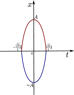
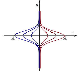
(a)	(b)

Figure 1. (a) Two solutions of equation (1). (b) Phase-portrait of system (2).

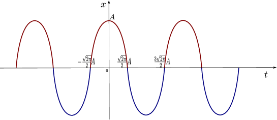
Figure 2. A weak $\mathcal{C}^{0}$-periodic solution of (1).

From (6) we introduce the ${\mathcal{C}}^{0}$-function, defined on the whole $\mathbb{R}$, as

$$\phi(t)=\begin{cases}(-1)^{n}\phi_{0}(t-n\sqrt{2}\pi),\quad\mbox{for}\quad t\in\left(\frac{2n-1}{2}\sqrt{2\pi},\frac{2n+1}{2}\sqrt{2\pi}\right),\quad n\in\mathbb{Z},\\ \qquad\quad 0\qquad\qquad\qquad\,\,\mbox{for}\quad t=\frac{2n+1}{2}\sqrt{2\pi},\qquad n\in\mathbb{Z},\end{cases}$$

see Figure 2. It is a $\mathcal{C}^{0}$-periodic function of period $T(A)=2\sqrt{2\pi}A$ and $x=\phi(t)$ satisfies (1), for all $t\in\mathbb{R}\setminus\cup_{n\in\mathbb{Z}}\{\frac{2n+1}{2}\sqrt{2\pi}\}.$ Hence $(i)$ of the theorem follows.

Notice that directly from (1), it is easy to see that this equation can not have $\mathcal{C}^{2}$-solutions such that $x(t^{*})=0$ for some $t^{*}\in\mathbb{R},$ because this would imply that $\lim_{t\to t^{*}}\ddot{x}(t)=\infty.$

$(ii)$ System (3) is Hamiltonian with Hamiltonian function

$$H(x,y)=\frac{y^{2}}{2}+\frac{\ln(x^{2}+k^{2})}{2}.$$

Since $\ln(x^{2}+k^{2})$ has a global minimum at $0$ and $\ln(x^{2}+k^{2})$ tends to infinity when $|x|$ does, system (3) has a global center at the origin. In Figure (3) we can see its phase portrait for some values of $k$. This figure also illustrates how the periodic orbits of (3) approach to the solutions of system (2).

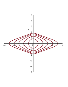
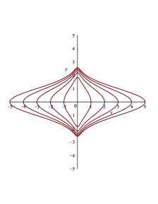
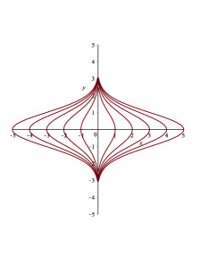
$k=1$	$k=\frac{1}{50}$	$k=\frac{1}{1000}$

Figure 3. Phase portraits of (3) for different values of $k$.

Its period function is

$$T(A;k)=2\int_{-A}^{A}\frac{dx}{y(x)}=2\int_{-A}^{A}\frac{dx}{\sqrt{2h-\ln{(x^{2}+k^{2})}}},$$

where $h=\ln(A^{2}+k^{2})/2$ is the energy level of the orbit passing through the point $(A,0)$. Therefore,

$$T(A;k)=2\int_{-A}^{A}\frac{dx}{\sqrt{\ln{\left(\frac{A^{2}+k^{2}}{x^{2}+k^{2}}\right)}}}=4\,A\int_{0}^{1}\frac{ds}{\sqrt{\ln{\left(\frac{A^{2}+k^{2}}{A^{2}s^{2}+k^{2}}\right)}}},$$

where we have used the change of variable $s=x/A$ and the symmetry with respect to $x.$ Then,

$$\lim_{k\rightarrow 0}T(A;k)=\lim_{k\rightarrow 0}\int_{0}^{1}\frac{4\,A\,ds}{\sqrt{\ln{\left(\frac{A^{2}+k^{2}}{A^{2}s^{2}+k^{2}}\right)}}}.$$

If we prove that

$$\lim_{k\rightarrow 0}\int_{0}^{1}\frac{4\,A\,ds}{\sqrt{\ln{\left(\frac{A^{2}+k^{2}}{A^{2}s^{2}+k^{2}}\right)}}}=\int_{0}^{1}\lim_{k\rightarrow 0}\frac{4\,A\,ds}{\sqrt{\ln{\left(\frac{A^{2}+k^{2}}{A^{2}s^{2}+k^{2}}\right)}}},$$ (9)

then

$$\lim_{k\rightarrow 0}T(A;k)=4\,A\,\int_{0}^{1}\frac{ds}{\sqrt{-2\ln{\left({s}\right)}}}=2\sqrt{2\pi}A=T(A)$$

and the theorem will follow. Therefore, for completing the proof, it only remains to show that (9) holds. For proving that, take any sequence $1/z_{n},$ with $z_{n}$ tending monotonically to infinity, and consider the functions $f_{n}(s)=\left(\ln{\left(\frac{A^{2}z_{n}^{2}+1}{A^{2}z_{n}^{2}s^{2}+1}\right)}\right)^{-1/2}.$ We have that the sequence $\{f_{n}(s)\}_{n\in\mathbb{N}}$ is formed by measurable and positive functions defined on the interval $(0,1)$. It is not difficult to prove that it is a decreasing sequence. In particular, $f_{n}(s)<f_{1}(s)$ for all $n>1$. Therefore, if we show that $f_{1}(s)$ is integrable, then we can apply the Lebesgue’s dominated convergence theorem ([10]) and (9) will follow. To prove that $\int_{0}^{1}f_{1}(s)<\infty$ note that for $s$ close to 1,

$$f_{1}(s)=\left(\ln{\left(\frac{A^{2}z_{1}^{2}+1}{A^{2}z_{1}^{2}s^{2}+1}\right)}\right)^{-1/2}\sim\left(\frac{2A^{2}z_{1}^{2}(1-s)}{A^{2}z_{1}^{2}+1}\right)^{-1/2}.$$

Since this last expression is integrable the result follows by the comparison test for improper integrals.

3. The Harmonic Balance Method

This section gives a brief description of the HBM applied the second order differential equations

$$\mathcal{F}:=\mathcal{F}(x(t),\ddot{x}(t))=0,$$ (10)

with $\mathcal{F}(-u,-v)=\mathcal{F}(u,v)$, and adapted to our interests. Notice that if $x(t)$ is a solution of (10) then $x(-t)$ also is a solution.

Suppose that equation (10) has a $T$-periodic solution $x(t)$ with initial conditions $x(0)=A$, $\dot{x}(0)=0$ and period $T=T(A).$ If $x(t)$ satisfies $x(t)=x(-t)$ it is clear that its Fourier series has no sinus terms and writes as

$$\sum_{k=1}^{\infty}a_{k}\cos(k\omega t),\quad\mbox{with}\quad\sum_{k=1}^{\infty}a_{k}=A\quad\mbox{and}\quad\omega=\frac{2\pi}{T}.$$

As we have seen in previous section, the weak periodic solutions of equation $x(t)\ddot{x}(t)+1=0$ that we want to approach satisfy the above property. Moreover $x(T/4)=0$ and $\dot{x}(T/4)$ does not exist. In any case, if we are searching smooth approximations to this $x(t)$, they should also satisfy $\dot{x}(t)\ddot{x}(t)+x(t)\dddot{x}(t)=0,$ and hence $\dot{x}(T/4)=0.$ For this reason, in this work we will search Fourier series in cosinus, not having the even terms $\cos(2j\omega t)$, $j\in\mathbb{N}\cup\{0\},$ which do not satisfy this property. This type of a priori simplifications are similar to the ones introduced in [6] for other problems.

Hence, in our setting, the HBM of order $N$ follows the next five steps:

1. Consider a trigonometric polynomial

$$x_{{}_{N}}(t)=\sum_{j=1}^{N}a_{2j-1}\cos((2j-1)\omega_{N}t)\quad\mbox{with}\quad\sum_{j=1}^{N}a_{2j-1}=A.$$ (11)

2. Compute the $2\pi/\omega_{N}$-periodic function $\mathcal{F}_{N}:=\mathcal{F}(x_{{}_{N}}(t),\ddot{x}_{{}_{N}}(t))$, which has also an associated Fourier series,

$$\mathcal{F}_{N}(t)=\sum_{j\geq 0}\mathcal{A}_{j}\cos(j\,\omega_{N}t),$$

where $\mathcal{A}_{j}=\mathcal{A}_{j}({\mathbf{a}},\omega_{N},A)$ $j\geq 0,$ with ${\mathbf{a}}=(a_{1},a_{3},\ldots,a_{{2N-1}})$.

3. Find all values ${\bf a}$ and $\omega_{N}$ such that

$$\mathcal{A}_{j}({\bf a},\omega_{N},A)=0\qquad\mbox{for}\quad 1\leq j\leq j_{N},$$ (12)

where $j_{N}$ is the value such that (12) consists exactly of $N$ non trivial equations. Notice also that each equation $\mathcal{A}_{j}({\bf a},\omega_{N},A)=0$ is equivalent to

$$\int_{0}^{2\pi/\omega_{N}}\cos(j\omega_{N}t)\mathcal{F}_{N}(t)\,dt=0.$$ (13)

4. Then the expression (11), with the values of ${\bf a}={\bf a}(A)$ and $\omega_{N}=\omega_{N}(A)$ obtained in point 3, provide candidates to be approximations of the actual periodic solutions of the initial differential equation. In particular, the functions $\mathcal{T}_{N}=\mathcal{T}_{N}(A)=2\pi/\omega_{N}$ give approximations of the periods of the corresponding periodic orbits.

5. Choose, as final approximation, the one associated to the solution that minimizes the norm

$$||\mathcal{F}_{N}(t)||=\int_{0}^{\mathcal{T}_{N}}\mathcal{F}_{N}^{2}(t)\,dt.$$

Remark 3.1.

(i) Notice that going from order $N$ to order $N+1$ in the method, implies to compute again all the coefficients of the Fourier polynomial, because in general the common Fourier coefficients of $x_{{}_{N}}(t)$ and $x_{{}_{N+1}}(t)$ do not coincide.

(ii) The above set of equations (12) is a system of polynomial equations which usually is not easy to solve. For this reason in many works, see for instance [7, 9] and the references therein, only the values of $N=1,2$ are considered. For solving system (12) for $N\geq 3$ we use the Gröbner basis approach $($[3]$)$. In general this method is faster that using successive resultants and moreover it does not give spurious solutions.

(iii) As far as we know, the test proposed in point 5 to select the best approach is not commonly used. We propose it following the definition of accuracy of an approximated solution used in [4] and inspired in the classical works [11, 12].

4. Application of the HBM

We start proving a lemma that will allow to reduce our computations to the case $A=1.$

Lemma 4.1.

Let $\mathcal{T}_{N}(A;m)$ be the period of the truncated Fourier series obtained applying the $N$-th order HBM to equation (4). Then there exists a real constant $C_{N}(m)$ such that $\mathcal{T}_{N}(A;m)=C_{N}(m)A$.

Proof.

Consider $\mathcal{F}_{N}=x_{N}^{m+1}\ddot{x}_{N}+x_{N}^{m}=0$, with $x_{N}$ given in (11). We have to solve the set of $N+1$ non-trivial equations

$$\int_{0}^{2\pi/\omega_{N}}\cos(j\omega_{N}t)\mathcal{F}_{N}(t)\,dt=0\qquad 1\leq j\leq j_{N},\quad\quad\sum_{j=1}^{N}a_{2j-1}=A,$$ (14)

with $N+1$ unknowns $a_{1},a_{3},\ldots,a_{{2N-1}}$ and $\omega_{N}$ and $A\neq 0.$ The lemma clearly follows if we prove next assertion: $\tilde{a}_{1},\tilde{a}_{3},\ldots,\tilde{a}_{{2N-1}}$ and $\tilde{\omega}_{N}$ is a solution of (14) with $A=1$ if and only if $A\tilde{a}_{1},A\tilde{a}_{3},\ldots,A\tilde{a}_{{2N-1}}$ and $\tilde{\omega}_{N}/A$ is a solution of (14). This equivalence is a consequence of the fact that the change of variables $s=At$ writes the integral equation in (14) as

$$\frac{1}{A}\int_{0}^{2\pi A/\omega_{N}}\cos\Big{(}j\frac{\omega_{N}}{A}s\Big{)}\mathcal{F}_{N}\Big{(}\frac{s}{A}\Big{)}\,ds=0$$

and from the structure of the right hand side equation of (14). Hence, $\mathcal{T}_{N}(A;m)=\mathcal{T}_{N}(1;m)A=:C_{N}(m)A,$ as we wanted to prove. ∎

Proof of Theorem 1.2.

Due to the above lemma, in the application of the $N$-th order HBM, we can restrict our attention to the case $A=1.$

$(i)$ Following section 3, we consider $x_{1}(t)=\cos(\omega_{1}t)$ as the first approximation to the actual solution of the functional equation $\mathcal{F}(x(t),\ddot{x}(t))=x^{m+1}\ddot{x}+x^{m}=0$. Then

$$\mathcal{F}_{1}(t)=-\omega_{1}^{2}\cos^{m+2}(\omega_{1}t)+\cos^{m}(\omega_{1}t).$$

When $m=2k$ the above expression writes as

$$\mathcal{F}_{1}(t)=-\omega_{1}^{2}\cos^{2k+2}(\omega_{1}t)+\cos^{2k}(\omega_{1}t)=0.$$ (15)

Using (13) for $j=0$ we get

$$\int_{0}^{2\pi/\omega_{1}}\mathcal{F}_{1}(t)\,dt=-\omega_{1}^{2}{I}_{2k+2}+{I}_{2k}=0,$$ (16)

where ${I}_{2\ell}=\int_{0}^{2\pi/\omega_{1}}\cos^{2\ell}(\omega_{1}t)dt$. By using integration by parts we prove that $(2k+2){I}_{2k+2}=(2k+1){I}_{2k}.$ Combining this equality and (16) we obtain that

$$\omega_{1}=\sqrt{\frac{2k+2}{2k+1}},$$

or equivalently,

$$\mathcal{T}_{1}(A;m)=2\pi A\sqrt{\frac{2k+1}{2k+2}},$$

that in terms of $m$ coincides with (5). The case $m$ odd follows similarly. The only difference is that instead of condition (16) to find $\mathcal{T}_{1}(A;m)$ we have to impose that

$$\int_{0}^{2\pi/\omega_{1}}\cos(\omega_{1}t)\mathcal{F}_{1}(t)\,dt=0,$$

because $\int_{0}^{2\pi/\omega_{1}}\mathcal{F}_{1}(t)\,dt\equiv 0.$

$(ii)$ Case $m=0$. Consider the functional equation $\mathcal{F}(x(t),\ddot{x}(t))=x(t)\ddot{x}(t)+1=0.$

When $N=2$, we take an approximation $x_{2}(t)=a_{1}\cos(\omega_{2}t)+a_{3}\cos(3\omega_{2}t).$ The vanishing of the coefficients of 1 and $\cos(2\omega_{2}t)$ in the Fourier series of $\mathcal{F}_{2}$ provides the nonlinear system

$$1-\frac{1}{2}(a_{1}^{2}+9a_{3}^{2})\omega_{2}^{2} =0,$$

$$a_{1}+10a_{3} =0,$$

$$a_{1}+a_{3}-1 =0.$$

By solving it and applying point 5 in the HBM we get that $\omega_{2}=18/\sqrt{218}.$ Therefore,

$$\mathcal{T}_{2}(A;0)=\frac{\sqrt{218}}{9}\pi A\approx 5.1539A,$$

as we wanted to prove.

For the third-order HBM we use as approximate solution $x_{3}(t)=a_{1}\cos(\omega_{3}t)+a_{3}\cos(3\omega_{3}t)+a_{5}\cos(5\omega_{3}t).$ Imposing that the coefficients of 1, $\cos(2\omega_{3}t)$, and $\cos(4\omega_{3}t)$ in $\mathcal{F}_{3}$ vanish we arrive at the system

$$P =2-\left(a_{1}^{2}+9a_{3}^{2}+25a_{5}^{2}\right)\omega_{3}^{2}=0,$$

$$Q =a_{1}^{2}+10a_{1}a_{3}+34a_{3}a_{5}=0,$$

$$R =5a_{3}+13a_{5}=0,$$

$$S =a_{1}+a_{3}+a_{5}-1=0.$$

Since all the equations are polynomial, the searching of its solutions can be done by using the Gröbner basis approach, see [3]. Recall that the idea of this method consists in finding a new systems of generators, say $G_{1},G_{2},\ldots,G_{\ell},$ of the ideal of $\mathbb{R}[a_{1},a_{3},a_{5},\omega_{3}]$ generated by $P,Q,R$ and $S$. Hence, solving $P=Q=R=S=0$ is equivalent to solve $G_{i}=0,$ $i=1,\ldots,\ell$. In general, choosing the lexicographic ordering in the Gröbner basis approach, we get that the polynomials of the equivalent system have triangular structure with respect to the variables and it can be easily solved.

Now, by computing the Gröbner basis of $\{P,Q,R,S\}$ with respect to the lexicographic ordering $[a_{1},a_{3},a_{5},\omega_{3}]$ we obtain a new basis with four polynomials ($\ell=4$), being one of them,

$$G_{1}(\omega_{3})=1553685075\omega_{3}^{8}-3692301106\omega_{3}^{6}+2143547654\omega_{3}^{4}-402413472\omega_{3}^{2}+20301192.$$

Solving $G_{1}(\omega_{3})=0$ and using again point 5 of our approach to HBM we get that the solution that gives the better approximation is

$$\omega_{3}=\frac{3\sqrt{5494790257313+115642506449\sqrt{715}}}{6905267}.$$

Hence the expression $\mathcal{T}_{3}(A;0)=2\pi A/\omega_{3}$ of the statement follows.

When $N=4$ we consider $x_{4}(t)=a_{1}\cos(\omega_{4}t)+a_{3}\cos(3\omega_{4}t)+a_{5}\cos(5\omega_{4}t)+a_{7}\cos(7\omega_{4}t),$ and we arrive at the system

$$P =2-\left(a_{1}^{2}+9a_{3}^{2}+25a_{5}^{2}+49a_{7}^{2}\right)\,\omega_{4}^{2}=0,$$

$$Q =a_{1}^{2}+10a_{1}a_{3}+34a_{3}a_{5}+74a_{5}a_{7}=0,$$

$$R =5a_{1}a_{3}+13a_{1}a_{5}+29a_{3}a_{7}=0,$$

$$S =9a_{3}^{2}+50a_{1}a_{7}+26a_{1}a_{5}=0,$$

$$U =a_{1}+a_{3}+a_{5}+a_{7}-1=0.$$

The Gröbner basis of $\{P,Q,R,S,U\}$ with respect to the lexicographic ordering $[a_{1},a_{3},a_{5},a_{7},\omega_{4}]$ is a new basis with five polynomials, being one of them an even polynomial in $\omega_{4}$ of degree 16 with integers coefficients. Solving it we obtain that the best approximation is $\omega_{4}\approx{1.2453},$ which gives $\mathcal{T}_{4}(A;0)\approx 5.0455\,A.$

For $N=5$ and $N=6$ we have done similar computations. In the case $N=5$ one of the generators of the Gröbner basis is an even polynomial in $\omega_{5}$ with integers coefficients and degree 32. When $N=6$ the same happens but with a polynomial of degree 64 in $\omega_{6}$. Solving the corresponding polynomials we get that $\omega_{5}\approx 1.2606$ and $\omega_{6}\approx 1.2501$, and consequently, $\mathcal{T}_{5}(A;0)\approx 4.9843\,A,$ and $\mathcal{T}_{6}(A;0)\approx 5.0260\,A.$

$(iii)$ Case $m=1$. We apply the HBM to $\mathcal{F}(x(t),\ddot{x}(t))=x^{2}(t)\ddot{x}(t)+x(t)=0.$

When $N=2,$ doing similar computations that in item $(ii)$, we arrive at

$$P =4-\left(3a_{1}^{2}+11a_{1}a_{3}+38a_{3}^{2}\right)\,\omega_{2}^{2}=0,$$

$$Q =4a_{3}-\left(a_{1}^{3}+22a_{1}^{2}a_{3}+27a_{3}^{3}\right)\omega_{2}^{2}=0,$$

$$R =a_{1}+a_{3}-1=0.$$

Again, by searching the Gröbner basis of $\{P,Q,R\}$ with respect to the lexicographic ordering $[a_{1},a_{3},\omega_{2}]$ we obtain a new basis with three polynomials, being one of them

$$G_{1}(\omega_{2})=7635411\omega_{2}^{8}-14625556\omega_{2}^{6}+5833600\omega_{2}^{4}-661376\omega_{2}^{2}+13824.$$

Notice that the equation $G(\omega_{2})=0$ can be algebraically solved. Nevertheless, for the sake of shortness, we do not give the exact roots. Following again step 5 of our approach we get that the best solution is $\omega_{2}\approx 1.1915$, or equivalently that $\mathcal{T}_{2}(A;1)\approx 5.2733A.$

The HBM when $N=3$ produces the system

$$P =4a_{1}-\left(3a_{1}^{3}+11a_{1}^{2}a_{3}+38a_{1}a_{3}^{2}+70a_{1}a_{3}a_{5}+102a_{1}a_{5}^{2}+43a_{3}^{2}a_{5}\right)\omega_{3}^{2}=0,$$

$$Q =4a_{3}-\left(a_{1}^{3}+22a_{1}^{2}a_{3}+27a_{1}^{2}a_{5}+70a_{1}a_{3}a_{5}+27a_{3}^{3}\right)\omega_{3}^{2}=0,$$

$$R =4a_{5}-\left(11a_{1}^{2}a_{3}+54a_{1}^{2}a_{5}+19a_{1}a_{3}^{2}+86a_{3}^{2}a_{5}+75a_{5}^{3}\right)\omega_{3}^{2}=0,$$

$$S =a_{1}+a_{3}+a_{5}-1=0.$$

Computing the Gröbner basis of $\{P,Q,R,S\}$ with respect to the lexicographic ordering $[a_{1},a_{3},a_{5},\omega_{3}]$ we get that one of the polynomials of the new basis is an even polynomial in $\omega_{3}$ of degree 26 with integer coefficients. By solving it we obtain that the best approximation is $\omega_{3}\approx 1.2206$, which produces the value $\mathcal{T}_{3}(A;1)$ of the statement.

When $N=4$ we arrive at five polynomial equations, that we omit. Once more, using the Gröbner basis approach we obtain a polynomial condition in $\omega_{4}$ of degree 80. Finally, $\omega_{4}\approx 1.2275$ and $\mathcal{T}_{4}(1;A)\approx 5.1186.$

$(iv)$ When $m=2$ we have to approach the solutions of $\mathcal{F}(x(t),\ddot{x}(t))=x^{3}(t)\ddot{x}(t)+x^{2}(t)=0.$ We do not give the details of the proof because we get our results by using exactly the same type of computations.

∎

Remark 4.2.

For each $N$ and $m$ our computations also provide a trigonometric polynomial that approaches the continuous weak periodic solution $\phi(t)$ given in the proof of Theorem 1.1.

Acknowledgements

The two authors are supported by the MICIIN/FEDER grant number MTM2008-03437, FEDER-UNAB10-4E-378 and the Generalitat de Catalunya grant number 2009-SGR 410. The first author is also supported by the grant FPU AP2009-1189.

References

- [1]
- [2] J. R. Acton, P. T. Squire, “Solving equations with Physical understanding”, Adam Hilger, Bristol and Boston, 1985.
- [3] D. Cox, J. Little, D. O’Shea,“Ideals, Varieties, and Algorithms: An Introduction to Computational Algebraic Geometry and Commutative Algebra”, Third edition. Undergraduate Texts in Mathematics. Springer, New York, 2007.
- [4] J. D. García-Saldaña, A. Gasull, A theoretical basis for the harmonic balance method, J. Differential Equations 254 (2013), no. 1, 67–80.
- [5] J. D. García-Saldaña, A. Gasull, The period function and the harmonic balance method, Preprint 2013.
- [6] R. E. Mickens, Fourier representations for periodic solutions of odd-parity systems, J. Sound Vibration 258 (2002), no. 2, 398–401.
- [7] R. E. Mickens, Harmonic balance and iteration calculations of periodic solutions to , J. Sound Vibration 306 (2007), no. 3-5, 968–972.
- [8] R. E. Mickens, “Oscillations in planar dynamic systems”, Series on Advances in Mathematics for Applied Sciences 37. World Scientific Publishing Co., Inc., River Edge, NJ, 1996.
- [9] R. E. Mickens, “Truly nonlinear oscillations. Harmonic balance, parameter expansions, iteration, and averaging methods”, World Scientific Publishing Co. Pte. Ltd., Hackensack, NJ, 2010.
- [10] W. Rudin, “Real and complex analysis”, third ed., McGraw-Hill Book Co., New York, 1987.
- [11] A. Stokes, On the approximation of nonlinear oscillations, J. Differential Equations 12 (1972), 535–558.
- [12] M. Urabe, Galerkin’s procedure for nonlinear periodic systems. Arch. Rational Mech. Anal. 20 (1965), 120–152.