Investigating a mixed action approach for $\eta$ and $\eta^{\prime}$ mesons in $N_{f}=2+1+1$ lattice QCD

Abstract:

We present results for a test of a mixed action approach with Osterwalder-Seiler valence quarks on a Wilson twisted mass sea for the example $\eta$, $\eta^{\prime}$ mesons. Flavour singlet pseudoscalar mesons obtain significant contributions from disconnected diagrams and are, therefore, expected to be particularly sensitive to mixed regularisations. We employ different procedures for matching valence and sea quark actions and show that the results agree in the continuum limit.

1 Introduction

Mixed action approaches, where valence and sea fermion actions are chosen differently, are used frequently in lattice QCD. They possess a number of important advantages compared to the so called unitary case, where valence and sea quark actions are identical. In particular, it is possible to use a valence action obeying more symmetries than the sea action in cases where the valence action cannot be used in the sea for theoretical reasons or because of too high computational costs. One can even go one step further and try to correct for small mismatches in bare parameters in the sea simulation by using a partially quenched mixed action approach.

Of course, a mixed action approach has also disadvantages, most prominently the breaking of unitarity, which might for instance drive certain correlators negative. Also, it is not clear a priori how big lattice artifacts one encounters in mixed formulations.

In this proceeding contribution we will present results on a mixed action approach with so called Osterwalder-Seiler [1] valence quarks on a $N_{f}=2+1+1$ flavour Wilson twisted mass sea [2] and compare to unitary results [3, 4, 5]. This particular action combination has the advantage that the flavour symmetry breaking present in the sea formulation is avoided in the valence formulation. Moreover, the matching of valence and sea actions is particularly simple [1]. As physical example we study the $\eta$ and $\eta^{\prime}$ system. The corresponding correlation functions obtain significant contributions from disconnected diagrams and are, therefore, uniquely sensitive to differences in between valence and sea formulations. We study the continuum limit with different matching conditions and find remarkably good agreement to the unitary case. First accounts of this work can be found in Ref. [8].

2 Lattice actions

The results we will present in this proceeding are obtained by evaluating gauge configuration provided by the European Twisted Mass Collaboration (ETMC) [9, 10, 11]. We use the ensembles specified in table 1 adopting the notation from Ref. [9]. More details can be found in this reference. All errors are computed using a blocked bootstrap procedure to account for autocorrelation.

The sea quark formulation is the Wilson twisted mass formulation with $N_{f}=2+1+1$ dynamical quark flavours. The Dirac operator for $u$ and $d$ quarks reads  [2]

$$D_{\ell}=D_{W}+m_{0}+i\mu_{\ell}\gamma_{5}\tau^{3}\,,$$ (1)

where $D_{W}$ denotes the standard Wilson operator and $\mu_{\ell}$ the bare light twisted mass parameter. For the heavy doublet of $c$ and $s$ quarks [12] the Dirac operator is given by

$$D_{h}=D_{W}+m_{0}+i\mu_{\sigma}\gamma_{5}\tau^{1}+\mu_{\delta}\tau^{3}\,,$$ (2)

with $\tau^{i}$ representing the Pauli matrices in flavour space. We remark that the twisted term introduces flavour mixing between strange and charm quarks that needs to be taken into account in the analysis.

The bare Wilson quark mass $m_{0}$ has been tuned to its critical value $m_{\mathrm{crit}}$ [13, 9] to achieve automatic order $\mathcal{O}\left(a\right)$ improvement [14], which is one of the main advantages of this formulation.

In the valence sector we employ the Osterwalder-Seiler (OS) action [1]. Formally, we introduce a twisted doublet both for valence strange and charm quarks [1, 15]. The Dirac operator for a single quark flavour $q\in\{s,c\}$

$$D_{q,q^{\prime}}=D_{W}+m_{\mathrm{crit}}\pm i\mu_{q}\gamma_{5}$$ (3)

is formally identical to the one in the light sector Eq. 1. Flavour $q$ ($q^{\prime}$) will come with $+\mu_{q}$ ($-\mu_{q}$). We denote the strange (charm) quark mass with $\mu_{s}$ ($\mu_{c}$). In Ref. [1] it was shown that automatic $\mathcal{O}(a)$-improvement stays valid and unitarity is restored in the continuum limit.

For matching the strange quark mass we employ two procedures based on meson masses. In previous studies it was found that matching kaon masses is best in the sense that the residual lattice artifacts in the results computed in a mixed framework are small [16]. The corresponding interpolating operator in the OS framework reads

$$\mathcal{O}_{K^{+}}=\bar{\psi}_{s}\ i\gamma_{5}\ \psi_{d}\,.$$ (4)

Note that we rely to the so called physical basis throughout this proceeding contribution [17]. For details on how to compute the kaon mass in the unitary case we refer to Ref. [10]. As a second matching observable we use the mass $M_{\eta_{s}}$ of the so-called $\eta_{s}$ meson – a pion made out of strange quarks which does not exist in nature. $M_{\eta_{s}}$ can be obtained from the connected only correlation function of the OS interpolating operator

$$\mathcal{O}_{\eta_{s}}=\frac{1}{\sqrt{2}}(\bar{\psi}_{s}\ i\gamma_{5}\ \psi_{s}+\bar{\psi}_{s^{\prime}}\ i\gamma_{5}\ \psi_{s^{\prime}})\,.$$ (5)

In both cases we tune the value of $a\mu_{s}$ such that the kaon ($\eta_{s}$) masses agree within error in between the mixed and the unitary formulation. In order to compute the matching values for $\mu_{s}$ we performed inversions in a range of $a\mu_{s}$ values around a first guess obtained from $\mu_{s}=\mu_{\sigma}-Z_{P}/Z_{S}\mu_{\delta}$, computed $M_{K^{+}}$ and $M_{\eta_{s}}$, and interpolated to the matching point where needed. The matching values for $a\mu_{s}$ for the two matching observables and all ensembles can be found in table 1.

The value of the charm quark mass turns out to be not very important for our investigation, because the charm does not contribute significantly to $\eta$ and $\eta^{\prime}$ mesons. Therefore, we use the following relations for the bare twisted quark mass parameters to obtain

$$\mu_{c}=\mu_{\sigma}\ +\ Z_{P}/Z_{S}\ \mu_{\delta}\,.$$ (6)

The value for the ratio of renormalisation constants can be found in Ref. [18]. The actual values for $\mu_{c}$ can again be found in table 1.

ensemble	$\beta$	$a\mu_{\ell}$	$a\mu_{\sigma}$	$a\mu_{\delta}$	$a\mu^{K^{+}}_{s}$	$a\mu^{\eta_{s}}_{s}$	$a\mu_{c}$	$L/a$	$N_{\mathrm{conf}}$
$A60.24$	$1.90$	$0.0060$	$0.150$	$0.190$	$0.0232$	$0.0138$	$0.2768$	$24$	$1177$
$B55.32$	$1.95$	$0.0055$	$0.135$	$0.170$	$0.0186$	$0.0110$	$0.2514$	$32$	$1964$
$D45.32sc$	$2.10$	$0.0045$	$0.0937$	$0.1077$	$0.0149$	$0.0118$	$0.1720$	$32$	$885$

Table 1: The ensembles used in this investigation. For the labeling we employ the notation of ref. [9]. Additionally, we give the number of the configurations $N_{\mathrm{conf}}$ which were used to compute correlators in light and strange quark sector, the mass of the OS valence strange quark $\mu_{s}$ for $M_{K^{+}}$ and $M_{\eta_{s}}$ matching and the OS valence charm quark mass $\mu_{c}$.

3 Pseudoscalar flavour-singlet mesons

In order to extract $\eta$ and $\eta^{\prime}$ states we compute the Euclidean correlation functions

$$\mathcal{C}(t)_{qq^{\prime}}=\langle\mathcal{O}_{q}(t^{\prime}+t)\mathcal{O}_{q^{\prime}}(t^{\prime})\rangle\,,\quad q,q^{\prime}\in\{u,s,c\}\,,$$ (7)

with operators $\mathcal{O}_{q}=(\bar{q}i\gamma_{5}q+\bar{q}^{\prime}i\gamma_{5}q^{\prime})/\sqrt{2}$, with $q\in\{u,s,c\}$ and identifying $u^{\prime}\equiv d$, again relying to the physical basis. The generalised eigenvalue problem is solved [19, 20, 21] for determining $M_{\eta}$ and $M_{\eta^{\prime}}$. Correlation functions are made of quark connected diagrams and disconnected quark loops. The quark connected pieces have been calculated via the so called “one-end-trick” [22] using stochastic timeslice sources and for the disconnected diagrams we resort to stochastic volume sources with complex Gaussian noise.

In the twisted mass formulation a very powerful variance reduction method is available for estimating the disconnected loop $(\bar{u}i\gamma_{5}u+\bar{d}^{\prime}i\gamma_{5}d^{\prime})/\sqrt{2}$, see Ref. [23]. In the OS case this variance reduction also applies to strange and charm disconnected loops [8]. Double counting of loops stemming from this approach needs to be taken into account by combinatorial factors.

Finally, we can define mixing angles $\phi_{l}$, $\phi_{s}$ in the quark flavour basis using the pseudoscalar matrix elements, see Ref. [3]. From chiral perturbation theory combined with large $N_{C}$ arguments $|\phi_{l}-\phi_{s}|/|\phi_{l}+\phi_{s}|\ll 1$ can be inferred according to Refs. [24, 25, 26, 27] which is confirmed by lattice QCD [4]. Therefore, we will consider only the average mixing angle

$$\tan^{2}\phi\equiv\frac{A_{l,\eta^{\prime}}A_{s,\eta}}{A_{l,\eta}A_{s,\eta^{\prime}}}\,,$$ (8)

where the $A_{q,n}=\langle 0|\bar{q}i\gamma_{5}q|n\rangle$ are pseudoscalar matrix elements determined from the eigenvectors with $n\in\{\eta,\ \eta^{\prime}\}$ and $q\in\{l,\ s\}$.

Excited State Removal

To improve the $\eta^{\prime}$ (and $\eta$) mass determinations, we use a method first proposed in Ref. [28], successfully applied for the $\eta_{2}$ (the $\eta^{\prime}$ in $N_{f}=2$ flavour QCD) in Ref. [23] and very recently to the $N_{f}=2+1+1$ case in Ref. [4]. It grounds on the assumption that disconnected contributions are significant only for the $\eta$ and $\eta^{\prime}$ state, but negligible for higher excited states. The method involves to subtract excited states from the connected correlators only. The subtracted connected and full disconnected are combined in $\mathcal{C}$, which is then used in the analysis. We refer to the discussion in Ref. [5, 4] for more details.

4 Results

In order to compare the mixed case with the unitary case we match the two actions as detailed in the previous sections using either the kaon or the $\eta_{s}$ mass. Next we compute $M_{\eta}^{\mathrm{OS}}$ at this matching points and the difference to the corresponding unitary masses $\Delta M_{\eta}$. At fixed values of $r_{0}M_{\pi}$ and $r_{0}M_{K}$ – which is approximately the case for the ensembles D45, B55 and A60, $r_{0}\Delta M_{\eta}$ should go to zero in the continuum limit with a rate of $\mathcal{O}(a^{2})$. We do not expect the small differences in $r_{0}M_{K}$ in between the different lattice spacing values to influence our results much, because unitary and OS data are affected likewise.

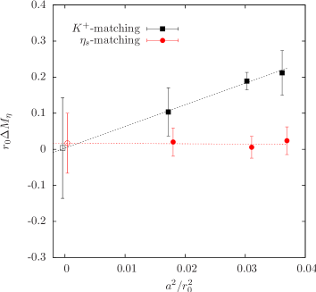
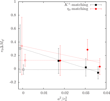
Figure 1: (a) We show $\Delta M_{\eta}$ for three ensembles (D45.32sc, B55.32, A60.24) as a function of the squared lattice spacing. Leftmost points correspond to linear continuum extrapolations indicated by the lines. (b) the same as (a) but for the $\eta^{\prime}$ state, for which we additionally show constant extrapolations.

$r_{0}\Delta M_{\eta}$ is shown in the left panel of figure 1 as a function of $a^{2}/r_{0}^{2}$. For both matching observables we observe a linear dependence in $a^{2}/r_{0}^{2}$. A corresponding continuum extrapolation in $a^{2}/r_{0}^{2}$ leads to the expected vanishing of this difference at $a=0$. Kaon matching clearly exhibits larger differences, while $\eta_{s}$ matching gives $r_{0}\Delta M_{\eta}$ compatible with zero for each value of the lattice spacing separately. This indicates smaller $a^{2}$ artifacts for $\eta_{s}$ matching because the unitary masses show constant scaling in $a^{2}$ [3]. $r_{0}M_{\eta^{\prime}}$ is shown in figure 1(b), which is in most cases compatible with zero even at finite lattice spacing. In the left panel of figure 2 we show $\Delta\phi$, again for both matching procedures, with the same conclusion.

As discussed in the introduction, one can correct for small mismatches in the bare simulation parameters used for the sea action by going slightly partially quenched in the valence sector. In order to test also this approach, we have tuned the respective $a\mu_{s}$ values for the ensembles D45, B55 and A60 such that all ensembles yield the same values of $r_{0}M_{K}=1.341$ or $r_{0}M_{\eta_{s}}=1.571$ .

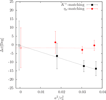
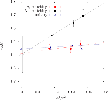
Figure 2: (a) We show $\Delta\phi$ for three ensembles (D45.32sc, B55.32, A60.24) as a function of the squared lattice spacing. Leftmost points correspond to linear continuum extrapolations indicated by the lines. (b) $r_{0}M_{\eta}$ as a function of $(a/r_{0})^{2}$ for the three ensembles. Different symbols correspond to two OS results with different matching conditions and to the unitary results. The leftmost points represent the corresponding continuum extrapolated values.

At these matching points we again compute $M_{\eta}$. In the right panel of figure 2 we show $r_{0}M_{\eta}$ as a function of $a^{2}/r_{0}^{2}$ for both matching conditions.We observe that, within statistical uncertainties, both matching procedures lead to the same continuum results.

A direct comparison to the unitary case is possible by also correcting the unitary values of $M_{\eta}$ for the small mismatch in the bare strange quark mass values. This is possible by measuring $dM_{\eta}^{2}/dM_{K}^{2}$ and use it to shift all $M_{\eta}$ values to the same value of $r_{0}M_{K}=1.341$ [3]. The result is again shown in the right panel of figure 2. The corresponding continuum extrapolation is linear in $a^{2}/r_{0}^{2}$ and also compatible to both OS continuum points within errors.

5 Conclusions and Outlook

We tested a mixed action approach with Osterwalder-Seiler valence quarks on a Wilson twisted mass sea for the $\eta$ and $\eta^{\prime}$ system. We expect this system to be most sensitive to different valence and sea discretisation due to significant disconnected contributions in the correlation functions.

We employed two different conditions to match valence and sea actions, using the kaon mass and the $\eta_{s}$ meson mass. For both matching procedures we observe agreement in the continuum limit, and in particular also with the unitary results. Moreover, we have also corrected for small mismatches in the bare strange quark mass value used in the gauge configuration generation, leading to a partially quenched mixed action approach. Also in this case we found within errors identical continuum extrapolated values for $M_{\eta}$ and the mixing angle $\phi$ for both matching procedures.

By correcting also the unitary values of $M_{\eta}$ we found agreement to the OS results. Therefore, we conclude that the mixed action approach can be used in the delicate case of the $\eta$ and $\eta^{\prime}$ meson, at least to the precision that we could achieve here.

We thank all members of ETMC for the most enjoyable collaboration. The computer time for this project was made available to us by the John von Neumann-Institute for Computing (NIC) on the JUDGE and Jugene systems. In particular we thank U.-G. Meißner for granting us access on JUDGE. This project was funded by the DFG as a project in the SFB/TR 16. K.O. and C.U. were supported by the BCGS of Physics and Astronomie. The open source software packages tmLQCD [29] and R [30] have been used.

References

- [1] R. Frezzotti and G. C. Rossi, JHEP 10, 070 (2004), arXiv:hep-lat/0407002.
- [2] ALPHA Collaboration, R. Frezzotti, P. A. Grassi, S. Sint and P. Weisz, JHEP 08, 058 (2001), hep-lat/0101001.
- [3] ETM Collaboration, K. Ottnad et al., JHEP 1211, 048 (2012), arXiv:1206.6719.
- [4] C. Michael, K. Ottnad and C. Urbach, Phys. Rev. Lett. 111, 181602 (2013), arXiv:1310.1207.
- [5] K. Ottnad et al., PoS LATTICE2013, 253 (2013).
- [6] E. B. Gregory, A. C. Irving, C. M. Richards and C. McNeile, PoS LAT2006, 176 (2006), arXiv:hep-lat/0610044.
- [7] UKQCD Collaboration, E. B. Gregory, A. C. Irving, C. M. Richards and C. McNeile, Phys.Rev. D86, 014504 (2012), arXiv:1112.4384.
- [8] K. Cichy et al., PoS LATTICE2012, 151 (2012), arXiv:1211.4497.
- [9] ETM Collaboration, R. Baron et al., JHEP 06, 111 (2010), arXiv:1004.5284.
- [10] ETM Collaboration, R. Baron et al., Comput.Phys.Commun. 182, 299 (2011), arXiv:1005.2042.
- [11] R. Baron et al., PoS LATTICE2010, 123 (2010), arXiv:1101.0518.
- [12] R. Frezzotti and G. C. Rossi, Nucl. Phys. Proc. Suppl. 128, 193 (2004), hep-lat/0311008.
- [13] T. Chiarappa et al., Eur. Phys. J. C50, 373 (2007), arXiv:hep-lat/0606011.
- [14] R. Frezzotti and G. C. Rossi, JHEP 08, 007 (2004), hep-lat/0306014.
- [15] ETM Collaboration, B. Blossier et al., JHEP 04, 020 (2008), arXiv:0709.4574.
- [16] S. R. Sharpe and J. M. Wu, Phys.Rev. D71, 074501 (2005), arXiv:hep-lat/0411021.
- [17] A. Shindler, Phys.Rept. 461, 37 (2008), arXiv:0707.4093.
- [18] ETM Collaboration, B. Blossier et al., PoS LATTICE2011, 233 (2011), arXiv:1112.1540.
- [19] C. Michael and I. Teasdale, Nucl.Phys. B215, 433 (1983).
- [20] M. Lüscher and U. Wolff, Nucl.Phys. B339, 222 (1990).
- [21] B. Blossier, M. Della Morte, G. von Hippel, T. Mendes and R. Sommer, JHEP 0904, 094 (2009), arXiv:0902.1265.
- [22] ETM Collaboration, P. Boucaud et al., Comput.Phys.Commun. 179, 695 (2008), arXiv:0803.0224.
- [23] ETM Collaboration, K. Jansen, C. Michael and C. Urbach, Eur.Phys.J. C58, 261 (2008), arXiv:0804.3871.
- [24] R. Kaiser and H. Leutwyler, arXiv:hep-ph/9806336.
- [25] R. Kaiser and H. Leutwyler, Eur.Phys.J. C17, 623 (2000), arXiv:hep-ph/0007101.
- [26] T. Feldmann, P. Kroll and B. Stech, Phys.Lett. B449, 339 (1999), arXiv:hep-ph/9812269.
- [27] T. Feldmann, P. Kroll and B. Stech, Phys.Rev. D58, 114006 (1998), arXiv:hep-ph/9802409.
- [28] H. Neff, N. Eicker, T. Lippert, J. W. Negele and K. Schilling, Phys.Rev. D64, 114509 (2001), arXiv:hep-lat/0106016.
- [29] K. Jansen and C. Urbach, Comput.Phys.Commun. 180, 2717 (2009), arXiv:0905.3331.
- [30] R Development Core Team, R: A language and environment for statistical computing, R Foundation for Statistical Computing, Vienna, Austria, 2005, ISBN 3-900051-07-0.