Application of beyond $\delta N$ formalism
–Varying sound speed–

Abstract

We focus on the evolution of curvature perturbation on superhorizon scales by adopting the spatial gradient expansion and show that the nonlinear theory, called the beyond $\delta N$-formalism as the next-leading order in the expansion. As one application of our formalism for a single scalar field, we investigate the case of varying sound speed. In our formalism, we can deal with the time evolution in contrast to $\delta N$-formalism, where curvature perturbations remain just constant, and nonlinear curvature perturbation follows the simple master equation whose form is similar as one in linear theory. So the calculation of bispectrum can be done in the next-leading order in the expansion as similar as the case of deriving the power spectrum. We discuss localized features of both primordial power and bispectrum generated by the effect of varying sound speed with a finite duration time. We can see a local feature like a bump in the equilateral bispectrum.

I Introduction

Recent observations of the cosmic microwave background anisotropy, such as WMAP and PLANCK satellites Ade:2013ktc ; Bennett:2012zja show very good agreement of the observational data with the prediction of standard inflationary cosmology where primordial fluctuations generated from quantum fluctuations of an inflaton field (see Lyth-book for review). The most recent observations by the PLANCK Ade:2013uln ; Ade:2013ydc show that the primordial curvature perturbation has nearly scale invariant and follows almost perfect Gaussian statistics. The non-Gaussianity of primordial fluctuations is a powerful probe to discriminate inflationary models and also distinguish among different models (see, e.g., Ref. CQG-focus-NG and references therein). Therefore, if any tiny signature from these observations will be detected, it can tell us important information on the physics behind inflation. The PLANCK data Ade:2013ydc have measured $-8.9<f^{loc}_{NL}<14.3$ and $-192<f^{eq}_{NL}<108$ for the so-called local type and equilateral type of non-Gaussianity, respectively, at the 2$\sigma$(95%) confidence level. These observations show that the primordial curvature perturbation follows almost perfect Gaussian statistics, however it may be detected at smaller scales and also as some tiny localized feature in the bispectrum. Especially, although the quantity $f_{NL}^{loc}$ is now constrained very strongly, the possibility still remains that non-Gaussianity of equilateral shape has localized features. If ever detected, it would tell us important properties of the curvature perturbation and be a probe to distinguish the models of inflation.

The gradient expansion approach Salopek:1990jq ; Nambu:1994hu ; Sasaki:1998ug ; Wands:2000dp ; Rigopoulos:2003ak ; Lyth:2005fi ; Takamizu:2010je ; Takamizu:2010xy ; Takamizu:2008ra ; Tanaka:2007gh ; Tanaka:2006zp ; Naruko:2012fe ; Takamizu:2013gy to discuss the evolution of nonlinear curvature perturbation on superhorizon scales is a powerful tool on calculation as well as the second-order perturbation theory Maldacena:2002vr ; Malik:2003mv . The lowest order in the expansion is the so-called $\delta N$-formalism Sasaki:1998ug ; Lyth:2005fi . But in order to analyzing local features of the equilateral bispectrum, this formula is not suitable since it leads to that nonlinearity of curvature perturbations on long-wavelength scales over horizon always generates the local shape of bispectrum. Therefore we focus on the nonlinear theory valid to the next-leading order in the expansion. It called the beyond $\delta N$-formalism and it is able to give us not only the local, but also the equilateral shape of bispectrum in contrast to $\delta N$-formalism, even though the expansion technique is taken on superhorizon scales Takamizu:2010xy ; Naruko:2012fe . Our nonlinear theory of the next-leading order in the expansion includes such subhorizon effect corresponding to the equilateral shape by matching a superhorizon curvature perturbation and subhorizon one suitably.

The main purpose of this paper is to investigate the situation where effective sound speed changes with a finite duration time and analyze whether features can appear in the bispectrum, in particular of the equilateral shape by using our nonlinear perturbation theory. The previous papers have studied the models of varying sound speed both in the power spectrum and in the bispectrum Khoury:2008wj ; Park:2012rh ; Ribeiro:2012ar ; Emery:2012sm ; Achucarro:2012fd ; Nakashima:2010sa ; Bartolo:2013exa ; Achucarro:2013cva (See also e.g., Achucarro:2010da ; Saito:2012pd ; Saito:2013aqa for the heavy physics, related to the same purpose and references therein), where one basically assumed a sudden change, however, we particularly focus on the effect of a finite duration time. As a simple application of beyond $\delta N$-formalism, we will consider a single scalar field whose effective sound speed will change in time due to a non-canonical kinetic term. As a first step, we will assume the background evolution follows a simple slow-roll inflation, although more realistic situation would be realized for a more complicated coupled kinetic term on multi-scalar system, such as the curvaton scenario Moroi:2001ct ; Lyth:2001nq , otherwise the slow-roll conditions will be also violated. However in this paper in order to extract the effects of the change of sound speed alone, we study the case of varying sound speed without affecting the background evolution as a simple tractable example, as same setup as in Ref. Nakashima:2010sa and see the appendix therein for more detailed discussion.

The rest of the paper is organized as follows. In Sec. II, we review beyond $\delta N$-formalism and especially, focus on the point that the master equations of curvature perturbation in linear and nonlinear theory show similar forms and derive the calculations. Then we discuss the possible example as the case of varying sound speed in Sec. III and derive featured power spectrums and bispectra of the curvature perturbations affected by such changes. Section IV is devoted to the conclusion.

II Beyond $\delta N$-Formalism

The gradient expansion technique has been applied up to second order in the expansion to a universe dominated by a single Tanaka:2006zp ; Tanaka:2007gh ; Takamizu:2008ra ; Takamizu:2010xy and multi-scalar field Naruko:2012fe , yielding the formalism “beyond $\delta N$”. The formulae have been also extended to be capable of a universe filled with a most generic non-canonical scalar field Takamizu:2013gy , which can give the so-called G-inflation. In this paper, we will consider a single scalar field as a simple example, whose kinetic term is a non-canonical, whose Lagrangian takes the form; $P(X,\phi)$ where $X=-\partial^{\mu}\phi\partial_{\mu}\phi/2$ because we will later discuss the situation the effective sound speed: $c_{s}^{2}=P_{X}/(P_{X}+2P_{XX}X)$ changes in time where the subscript $X$ represent derive with respect to $X$ and notice that the Lagrangian denoted by $P$ plays the role of the pressure as shown in Ref Takamizu:2008ra ; Christopherson:2008ry .

Following Ref. Takamizu:2010xy , we will briefly review beyond $\delta N$-formalism for a single scalar field in this section. This system is characterized by a single scalar degree of freedom, and hence one expects that a single master variable governs the evolution of scalar perturbations even at nonlinear order. By virtue of gradient expansion, one can indeed derive a simple evolution equation for an appropriately defined master variable ${\cal R}_{c}^{\rm NL}$ on comoving hypersurfaces:

$${{\cal R}_{c}^{\rm NL}}^{\prime\prime}+2{z^{\prime}\over z}{{\cal R}_{c}^{\rm NL}}^{\prime}+{c_{s}^{2}\over 4}\,R^{(2)}[\,{\cal R}_{c}^{\rm NL}\,]={\cal O}(\epsilon^{4})\,,$$ (1)

with

$$z\equiv{a\over H}\left({\rho+P\over c_{s}^{2}}\right)^{1\over 2}\,,$$ (2)

where $\rho$ and $P$ denote energy density and pressure of a scalar field, respectively, the prime represents differentiation with respect to the conformal time $\tau$, $\epsilon$ is the small expansion parameter, and $R^{(2)}[X]$ is the Ricci scalar of the metric $X$. Hereafter we attach the superscript $(m)$ to a quantity of order of gradient expansion: ${\cal O}(\epsilon^{m})$ and take the metric as

$$ds^{2}=a^{2}(-\alpha^{2}d\tau^{2}+e^{2\ell}\delta_{ij}dx^{i}dx^{j})+{\cal O}(\epsilon^{3})\,,$$ (3)

where $\alpha$ denotes the lapse function, while the shift vector is vanishing at the next-leading order $\beta^{i}={\cal O}(\epsilon^{3})$, then $R^{(2)}[X]$ can be given by

$$R^{(2)}[\ell^{(0)}]=\,{-2(2\Delta\ell^{(0)}+\delta^{ij}\partial_{i}\ell^{(0)}\partial_{j}\ell^{(0)})e^{-2\ell^{(0)}}}\,.$$ (4)

The equation (1) is to be compared with its linear counterpart:

$${{\cal R}^{\rm Lin}_{c}}^{\prime\prime}+2{z^{\prime}\over z}{{\cal R}^{\rm Lin}_{c}}^{\prime}-c_{s}^{2}\,\Delta{\cal R}^{\rm Lin}_{c}=0\,,$$ (5)

from which one notices the correspondence between the linear and nonlinear evolution equations. In order to calculate the evolution equations in Fourier space, we have to take the replacement $\Delta\to-k^{2}$.

It is important notice that the structures of both (1) and (5) are similar forms, except for last terms in the left hand sides. This point is advantage in order to estimate evolutions of curvature perturbations in linear and nonlinear theory since same calculation is valid on following the evolution equation. We will see the details later.

II.1 Linear Theory valid up to ${\cal O}(\epsilon^{2})$

To obtain the power spectrum, we will use the linear theory of the curvature perturbation in this subsection. The above equation (5) has two independent solutions; conventionally called a growing mode and a decaying mode. We assume that the growing mode is constant in time at leading order in the spatial gradient expansion.

As shown in Takamizu:2010xy , the linear solution valid up to ${\cal O}(\epsilon^{2})$ can be obtained as

$${\cal R}_{c,\bm{k}}^{\rm Lin}(\tau) = \Bigl{[}\tilde{\alpha}^{\rm Lin}_{\bm{k}}+(1-\tilde{\alpha}^{\rm Lin}_{\bm{k}}){\tilde{D}(\tau)\over\tilde{D}_{*}}$$ (6)

$$-\left({\tilde{F}_{*}\over\tilde{D}_{*}}\tilde{D}(\tau)+\tilde{F}(\tau)\right)k^{2}\Bigr{]}U^{(0)}_{\bm{k}}\,,$$

where the integrals $\tilde{D}(\tau)$ and $\tilde{F}(\tau)$ have been given as

$$\tilde{D}(\tau) = 3{\cal H}(\tau_{*})\int_{\tau_{*}}^{\eta}d\tau^{\prime}{z^{2}(\tau_{*})\over z^{2}(\tau^{\prime})},$$

$$\tilde{F}(\tau) = \int_{\tau_{*}}^{\tau}\frac{d\tau^{\prime}}{z^{2}(\tau^{\prime})}\int_{\tau_{*}}^{\tau^{\prime}}z^{2}(\tau^{\prime\prime})c_{s}^{2}(\tau^{\prime\prime})d\tau^{\prime\prime}.$$ (7)

Here $\tilde{D}_{*}=\tilde{D}(\tau_{*}),\tilde{F}_{*}=\tilde{F}(\tau_{*})$, $\tau_{*}$ and $\cal H$ denote an initial time of gradient expansion and the conformal Hubble parameter ${\cal H}=d\ln a/d\tau$, respectively. The integrals in (7) represent a decaying and growing mode solution, respectively.

Note that ${\cal R}^{\rm Lin}_{c,_{\bm{k}}}(\tau_{*})=U^{(0)}_{\bm{k}}$ that is just a constant solution, while ${\cal R}^{\rm Lin}_{c,_{\bm{k}}}(0)=\tilde{\alpha}^{\rm Lin}_{\bm{k}}U^{(0)}_{\bm{k}}$. Thus if the factor $|\tilde{\alpha}^{\rm Lin}_{\bm{k}}|$ is large, it represents an enhancement of the curvature perturbation on superhorizon scales due the ${\cal O}(\epsilon^{2})$ effect.

Here it is useful to consider an explicit expression for $\tilde{\alpha}^{\rm Lin}_{\bm{k}}$ in terms of ${\cal R}^{\rm Lin}_{c,{\bm{k}}}$ and its derivative at $\tau=\tau_{*}$. The result is

$$\tilde{\alpha}^{\rm Lin}_{\bm{k}}=1+{\tilde{D}_{*}\over 3{\cal H}_{*}}\frac{{{\cal R}^{\rm Lin}_{c,_{\bm{k}}}}^{\prime}(\tau_{*})}{{\cal R}^{\rm Lin}_{c,_{\bm{k}}}(\tau_{*})}-k^{2}\tilde{F}_{*}+{\cal O}(k^{4}).$$ (8)

In order to relate our calculation with the standard formula for the curvature perturbation in linear theory, we introduce $\tau_{k}$ (or $t_{k}$) which denotes the time at which the comoving wavenumber has crossed the Hubble horizon,

$$\tau_{k}=-{r\over k}\,;\quad 0<r\ll 1\,.$$ (9)

The power spectrum at the horizon crossing time is given by

$$\langle{\cal R}^{\rm Lin}_{c,\bm{k}}(\tau_{k}){\cal R}^{\rm Lin}_{c,\bm{k}^{\prime}}(\tau_{k^{\prime}})\rangle=(2\pi)^{3}P_{{\cal R}}(k)\delta^{3}(\bm{k}+\bm{k}^{\prime}),$$

$$P_{{\cal R}}(k)=\left|{\cal R}^{\rm Lin}_{c,\bm{k}}(\tau_{k})\right|^{2}\,.$$ (10)

By inverting ${\cal R}^{\rm Lin}_{c,\bm{k}}$ in terms of $U^{(0)}_{\bm{k}}$ as shown in Takamizu:2010xy , we can show the final value of the linear curvature perturbation as

$${\cal R}^{\rm Lin}_{c,\bm{k}}(0)=\tilde{\alpha}^{\rm Lin}_{\bm{k}}U^{(0)}_{\bm{k}}={\alpha}^{\rm Lin}_{\bm{k}}{\cal R}^{\rm Lin}_{c,\bm{k}}(\tau_{k})+{\cal O}(k^{4})\,,$$ (11)

where

$${\alpha}^{\rm Lin}_{\bm{k}}=1+\alpha^{\cal R}{D}_{k}-k^{2}{F}_{k}\,,$$ (12)

and

$$\alpha^{\cal R} = \frac{1}{3{\cal H}(\eta_{k})}{{\cal R^{\rm Lin}}^{\prime}_{c,\bm{k}}\over{\cal R}^{\rm Lin}_{c,\bm{k}}}\bigg{|}_{\tau=\tau_{k}},$$

$${D}_{k} = 3{\cal H}(\tau_{k})\int_{\tau_{k}}^{0}d\tau^{\prime}{z^{2}(\tau_{k})\over z^{2}(\tau^{\prime})},$$

$${F}_{k} = \int_{\tau_{k}}^{0}\frac{d\tau^{\prime}}{z^{2}(\tau^{\prime})}\int_{\tau_{k}}^{\tau^{\prime}}z^{2}(\tau^{\prime\prime})c_{s}^{2}(\tau^{\prime\prime})d\tau^{\prime\prime}.$$ (13)

The formula (11) will be used in the next subsection.

The power spectrum at the final time is thus enhanced by the factor $|{\alpha}^{\rm Lin}_{\bm{k}}|^{2}$ as

$$\langle{\cal R}^{\rm Lin}_{c,\bm{k}}(0){\cal R}^{\rm Lin}_{c,\bm{k}^{\prime\prime}}(0)\rangle=(2\pi)^{3}|{\alpha}^{\rm Lin}_{\bm{k}}|^{2}P_{{\cal R}}(k)\delta^{3}(\bm{k}+\bm{k}^{\prime})\,.$$ (14)

II.2 Nonlinear theory valid up to ${\cal O}(\epsilon^{2})$

Using the linear solution of the curvature perturbation given by (6), here we can derive the nonlinear solution by matching the two at $\tau=\tau_{*}$. The main purpose of the matching is to make it possible to analyze superhorizon nonlinear evolution valid up to the second order in gradient expansion, starting from a solution in the linear theory. In particular, we would like to evaluate the bispectrum induced by the superhorizon nonlinear evolution. For this purpose, we need to have full control over terms up not only to ${\cal O}(\epsilon^{2})$ but also to ${\cal O}(\delta^{2})$, where we suppose that the linear solution is of order ${\cal O}(\delta)$. Therefore, the matching condition at $\tau=\tau_{*}$ should be of the form

$${\cal R}^{\rm NL}_{c}(\tau_{*}) = {\cal R}^{\rm Lin}_{c}(\tau_{*})+s_{1}(\tau_{*})+{\cal O}(\epsilon^{4},\delta^{3}),$$

$${{\cal R}^{\rm NL}_{c}}^{\prime}(\tau_{*}) = {{\cal R}^{\rm Lin}_{c}}^{\prime}(\tau_{*})+s_{2}(\tau_{*})+{\cal O}(\epsilon^{4},\delta^{3})\,,$$ (15)

where $s_{1}(\tau_{*})={\cal O}(\delta^{2})$ and $s_{2}(\tau_{*})={\cal O}(\delta^{2})$ are functions of $\tau_{*}$ and spatial coordinates. While the linear solution ${\cal R}^{\rm Lin}_{c}(\tau)$ is considered as an input, i.e., initial condition, the additional terms, $s_{1}(\tau_{*})$ and $s_{2}(\tau_{*})$, are to be determined by the following condition. The terms of order ${\cal O}(\delta^{2})$ in ${\cal R}^{\rm NL}_{c,\bm{k}}$ and ${{\cal R}^{\rm NL}_{c,\bm{k}}}^{\prime}$ should vanish at the horizon crossing when $\tau=\tau_{k}$. Note that $\tau_{k}<\tau_{*}$. In other words, $s_{1}(\tau_{*})$ and $s_{2}(\tau_{*})$ represent the ${\cal O}(\delta^{2})$ part of ${\cal R}^{\rm NL}_{c}$ and ${{\cal R}^{\rm NL}_{c}}^{\prime}$, respectively, generated during the period between the horizon crossing time and the matching time.

We have to omit the explicit way to determine the terms $s_{1}$ and $s_{2}$ for want of space, that was shown in Takamizu:2010xy . As a result, using the linear solution of the curvature perturbation given by (6) we have the nonlinear comoving curvature perturbation at the final time $\tau=0$ (or $t=\infty$) given by

$${\cal R}_{c,\bm{k}}^{\rm NL}(0)={\cal R}^{\rm Lin}_{c,\bm{k}}(\tau_{k})-(1-{\alpha}^{\rm Lin}_{\bm{k}}){\cal R}^{\rm Lin}_{c,\bm{k}}(\tau_{k})$$

$$-\frac{1}{4}F_{k}\tilde{R}^{(2)}[{\cal R}^{\rm Lin}_{c}(\tau_{k})]+{\cal O}(\epsilon^{4},\delta^{3})\,,$$ (16)

where

$$\tilde{R}^{(2)}[\ell^{0}] \equiv-2(\delta^{ij}\partial_{i}\ell^{0}\partial_{j}\ell^{0}-4\ell^{0}\Delta\ell^{0})$$

$$=4\Delta\ell^{0}+R^{(2)}[\ell^{0}]+{\cal O}((\ell^{0})^{3})\,.$$ (17)

The first term in (16) corresponds to the result of the $\delta N$ formalism, that is a constant since we considered the system for a single scalar field, the second term is related to an enhancement on superhorizon scales in linear theory, and the last term is the nonlinear effect which may become important if $F_{k}$ is large.

Here we can notice that in order to the final values of curvature perturbation both in linear (11) and in nonlinear theory (16), all one have to do is to estimate the same integrals shown in both theories as $D_{K}$ and $F_{k}$ in $\alpha^{\rm Lin}_{\bm{k}}$. The reason why is that the master equations (1) and (5) for both theories have the same structures of evolution equation as described before.

In this subsection, we calculate the bispectrum of our nonlinear curvature perturbation by assuming that ${\cal R}^{\rm Lin}_{c,\bm{k}}(\tau_{k})$ is a Gaussian random variable. We assume the leading order contribution to the bispectrum comes from the terms second order in ${\cal R}^{\rm Lin}_{c,\bm{k}}(\tau_{k})$. The final result (16) can be reduced to

$$\zeta_{\bm{k}}={\cal R}^{\rm NL}_{c,\bm{k}}(0)$$

$$=\alpha^{\rm Lin}_{\bm{k}}\ {\cal R}^{\rm Lin}_{c,\bm{k}}(\tau_{k})+{F_{k}\over 2}\ \Biggl{\{}\int\frac{d^{3}k^{\prime}d^{3}k^{\prime\prime}}{(2\pi)^{3}}(4{k^{\prime}}^{2}-\delta_{ij}{k^{\prime}}^{i}{k^{\prime\prime}}^{j})$$

$$\times{\cal R}^{\rm Lin}_{c,\bm{k}^{\prime}}(\tau_{k^{\prime}}){\cal R}^{\rm Lin}_{c,\bm{k}^{\prime\prime}}(\tau_{k^{\prime\prime}})\delta^{3}(-\bm{k}+\bm{k}^{\prime}+\bm{k}^{\prime\prime})\Biggr{\}}$$

$$+{\cal O}(\epsilon^{4},\delta^{3})\,.$$ (18)

By assuming the Gaussian statistics for ${\cal R}^{\rm Lin}_{c,\bm{k}}(\tau_{k})$, it is easy to calculate the power spectrum shown as (14) with (10) and the bispectrum of primordial curvature perturbation: $\zeta$.

The dimensionless bispectrum ${\cal B}_{\zeta}$ is expressed in terms of the Fourier transformation of the three point function as

$$\left\langle{\zeta}_{{\bm{k}}_{1}}{\zeta}_{{\bm{k}}_{2}}{\zeta}_{{\bm{k}}_{3}}\right\rangle_{C}=(2\pi)^{7}\delta^{3}({\bf k}_{1}+{\bf k}_{2}+{\bf k}_{3}){\cal P}^{2}_{\zeta}{{\cal B}_{\zeta}\over k_{1}^{2}k_{2}^{2}k_{3}^{2}},$$ (19)

where $\langle\cdots\rangle_{C}$ means that it extracts out only connected graphs. We use the dimensionless quantity ${\cal B}_{\zeta}$ to represent the amplitude of the bispectrum with the uncorrected power spectrum ${\cal P}_{\zeta}$, which has been defined by ${\cal P}_{\zeta}=k^{3}P_{\zeta}/2\pi^{2}$. We can use a standard amplitude of dimensionless power spectrum as ${\cal P}_{\zeta}={\cal O}(10^{-9})$. With the help of (18), the three point correlation function of ${\zeta}$ is at leading order calculated as

$$\left\langle{\zeta}_{{\bm{k}}_{1}}{\zeta}_{{\bm{k}}_{2}}{\zeta}_{{\bm{k}}_{3}}\right\rangle_{C}=(2\pi^{3})\Biggl{[}Re(\alpha^{{\rm Lin}*}_{k_{1}}\alpha^{\rm Lin}_{k_{2}})F_{k_{3}}$$

$$\times\left\{2(k_{1}^{2}+k_{2}^{2})-\delta_{ij}k_{1}^{i}k_{2}^{j}\right\}\delta^{(3)}({\bf k}_{1}+{\bf k}_{2}+{\bf k}_{3})$$

$$\times|{\cal R}^{\rm Lin}_{c,\bm{k}_{1}}(\tau_{k_{1}})|^{2}|{\cal R}^{\rm Lin}_{c,\bm{k}_{2}}(\tau_{k_{2}})|^{2}+{\rm 2terms}\Biggr{]}\,,$$ (20)

where $Re$ means taking a real part, a superscript star denotes a complex conjugate and ‘2 terms’ means terms with cyclic and permutations among the three wavenumbers. The power spectrum of ${\cal R}^{\rm Lin}_{c,\bm{k}}(\tau_{k})$ is written as (10). Then we have

$${\cal B}_{\zeta}(k_{1},k_{2},k_{3})=\frac{1}{8k_{1}k_{2}k_{3}}\Biggl{[}Re(\alpha^{{\rm Lin}*}_{k_{1}}\alpha^{\rm Lin}_{k_{2}})F_{k_{3}}$$

$$\times\left\{5(k_{1}^{2}+k_{2}^{2})-k_{3}^{2}\right\}k_{3}^{3}\,\triangle{\cal P}_{{\zeta}}(k_{1})\triangle{\cal P}_{{\zeta}}(k_{2})$$

$$+{\rm 2terms}\Biggr{]}\,,$$ (21)

where $\triangle{\cal P}_{\zeta}$ denotes the modulation factor of power spectrum, that is a ratio of a corrected power spectrum to uncorrected one:

$$\triangle{\cal P}_{\zeta}(k)={k^{3}\over 2\pi^{2}{\cal P}_{\zeta}}\left|{\cal R}^{\rm Lin}_{c,\bm{k}}(\tau_{k})\right|^{2}\,.$$ (22)

III Application–varying sound speed–

We consider the case of varying sound speed as one application of beyond $\delta N$-formalism. As a simple example, we have assumed that the background evolution satisfies the slow-roll conditions throughout this paper, that is

$$\eta_{1}=-{\dot{H}\over H^{2}}\ll 1\ {\rm and}\ \eta_{2}={\dot{\eta}_{1}\over H\eta_{1}}\ll 1\,,$$ (23)

where a dot denotes a derivatives with respect to the physical time $t$. We compute the curvature perturbation for a model such that time variation of the sound speed is described by the following function as

$$c_{s}^{2}=c_{s1}^{2}+(c_{s2}^{2}-c_{s1}^{2}){\tanh[(\tau-\tau_{0})/d]+1\over 2}\,,$$ (24)

where $c_{s1},c_{s2},\tau_{0}$ and $d$ are parameters and the sound speed changes from $c_{s1}$ to $c_{s2}$ with a varying duration characterised by $\tau_{0}$ and $d$. We can introduce a new parameter $T=c_{s1}/c_{s2}$, which represents the ratio of sound speed before and after the transition. If we take the width of duration very small $d\mbox{\raisebox{-4.30554pt}{$\stackrel{{\scriptstyle\textstyle<}}{{\textstyle\sim}}$}}1$, the model results in the previous study of sudden varying sound speeds as in Nakashima:2010sa . Throughout this paper, we set $\tau_{0}=-500$, but the results do not depend on specifying the choice of the parameter. We plot the evolution of sound speed for example in Fig.1 where we set $T=0.9$ and $d=1,10,50,100$.

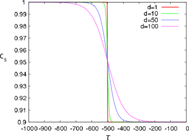
Figure 1: We plot varying sound speed as taking $c_{s1}=1,c_{s2}=0.9$ for various values of varying width $d$. We set $\tau_{0}=-500$. The horizontal axis is taking the conformal time.

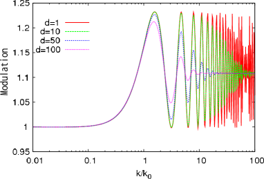
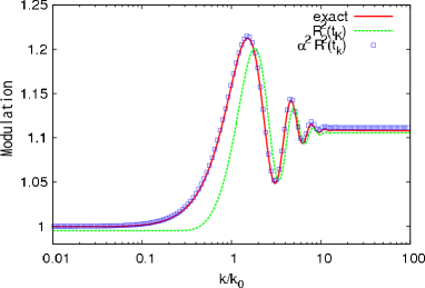
Figure 2: (Left) We plot the modulation factor of final power spectrum for various values of $d$ with setting $T=0.9$. We can see the featured bumps at $k=k_{0}$ with oscillation. As $d$ taking smaller value, the oscillations are more intensive. (Right) Comparison the long-wavelength approximation (14) with the numerical exact solution of (30). We set $T=0.9$ and $d=100$. The enhancement from the amplitude at the horizon crossing time ${\cal R}^{2}(\tau_{k})$(green line), which is described by $(\alpha^{\rm Lin}_{\bm{k}})^{2}$ of (12), occurs at superhorizon scales $k/k_{0}<1$.

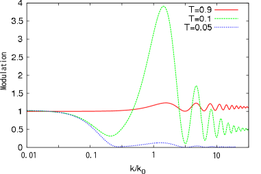
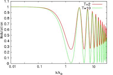
Figure 3: We plot the modulation of final power spectrums for various values of $T<1$(left) and $T>1$(right) with setting $d=20$. All cases in left(right) panel correspond to the situations of decreasing(increasing) sound speeds.

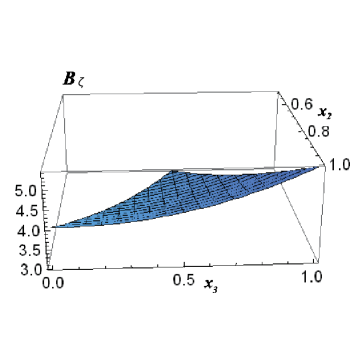
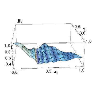
Figure 4: We plot dimensionless bispectrum as a function of $x_{2}=k_{2}/k_{1}$ and $x_{3}=k_{3}/k_{1}$. We set $T=0.5,d=20$ with parameters: $k_{1}/k_{0}=0.1$(left) and $k_{1}/k_{0}=1$(right). The bispectrum have a peak at the equilateral(local) shape in left(right) panel.

III.1 Power Spectrum

The basic equation in the linear theory for primordial curvature perturbation $\zeta$ is written in terms of $v=\zeta z$. The basic equation of motion for Fourier modes are given by

$$v_{k}^{\prime\prime}+\left(c_{s}^{2}k^{2}-\frac{z^{\prime\prime}}{z}\right)v_{k}=0\,.$$ (25)

We introduce a variable $u$, which is related to $v$ as

$$-c_{s}k^{2}u_{k}=z\left(\frac{v_{k}}{z}\right)^{\prime},\ \ c_{s}v_{k}=\theta\left(\frac{u_{k}}{\theta}\right)^{\prime}\,,$$ (26)

where we have defined $\theta\equiv{1}/{(c_{s}z)}$. The basic equation of motion (25) in terms of the Fourier modes $u_{k}$ is obtained as

$$u_{k}^{\prime\prime}+\left(c_{s}^{2}k^{2}-\frac{\theta^{\prime\prime}}{\theta}\right)u_{k}=0\,.$$ (27)

Note that the term $(c_{s}^{\prime}/c_{s})$ does not exist in $\theta^{\prime\prime}/\theta$ since the variable $\theta$ does not depend on $c_{s}$ from (2) as $\theta=1/(a\sqrt{2\eta_{1}})$. We have to solve this equation under the background evolution. The term $\theta^{\prime\prime}/\theta$ is rewritten in terms of slow-roll parameters as

$$\frac{\theta^{\prime\prime}}{\theta}=\frac{1}{\tau^{2}}\left(\frac{\eta_{2}}{2}-\eta_{1}\right)\,,$$ (28)

where we have used slow-roll approximation that is, $|\eta_{1}|,|\eta_{2}|\ll 1$ and taking their linear limits, and used a useful equation

$$aH=-\frac{1}{\tau(1-\eta_{1})}\,.$$ (29)

Therefore, we can obtain the basic equation

$$u_{k}^{\prime\prime}+\left(c_{s}^{2}k^{2}-\frac{\nu^{2}-\frac{1}{4}}{\tau^{2}}\right)u_{k}=0\,,$$ (30)

where we have defined

$$\nu^{2}=\frac{\eta_{2}}{2}-\eta_{1}+\frac{1}{4}\,,$$ (31)

and approximate it as

$$\nu=\sqrt{\frac{\eta_{2}}{2}-\eta_{1}+\frac{1}{4}}\approx\frac{1}{2}+\frac{\eta_{2}}{2}-\eta_{1}\,.$$ (32)

In the regime when $\tau<\tau_{0}$, setting $c_{s}=c_{s1}$ leads to the equation of motion

$$u_{k}^{\prime\prime}+\left(c_{s1}^{2}k^{2}-\frac{\nu^{2}-\frac{1}{4}}{\tau^{2}}\right)u_{k}=0\,,$$ (33)

and its solution is obtained by

$$u_{k1}=\sqrt{-kc_{s1}\tau}\left[c_{1}H_{\nu}^{(1)}(-kc_{s1}\tau)+c_{2}H_{\nu}^{(2)}(-kc_{s1}\tau)\right]\,,$$ (34)

where $H_{\nu}^{(1),(2)}(\tau)$ denote the Hankel function and $c_{1,2}$ are arbitrary constants, which have to be determined by initial conditions at the time $\tau\to-\infty$. We choose the adiabatic vacuum at the initial time in terms of $v_{k}$ as $v_{k}\to e^{-ikc_{s1}\tau}/{\sqrt{2kc_{s1}}}$. Hence it leads to the choice of $c_{1},c_{2}$ as

$$c_{1}=\frac{i}{2k^{3/2}}\sqrt{\frac{\pi}{c_{s1}}}\exp\left(\frac{2\nu+1}{4}\pi i\right),\ \ \ c_{2}=0\,.$$ (35)

We solve the basic equation (30) numerically with the above initial condition. This solution can show us the evolution from subhorizon scale to superhorizon scale. On the other hand, we can calculate the enhance factor $|\alpha^{\rm Lin}_{\bm{k}}|$ by estimating the equation (14) obtained under the long-wavelength approximation. Then we can compare it with the above numerical exact solution. In order to compare them, we have to estimate $\zeta$ from the numerical solution of $u$ by using the relation $\zeta=v/z=\theta^{2}(u/\theta)^{\prime}$.

First we will show the exact solution by using numerical solving in the left panel of Fig.2 for various values of $d$. We plot the modulation factors of power spectrum with $k/k_{0}$, where $k_{0}$ is the wavenumber corresponding to a transition time $\tau_{0}$. It shows some feature like bump at $k=k_{0}$ with oscillation. As $d$ taking smaller value, the oscillations are more intensive and they do not converge for $d<{\cal O}(1)$. The result of $d=1$ is consistent with the previous result of Ref.Nakashima:2010sa for studying the case of a sudden varying sound speed.

The right panel of Fig.2 shows the comparison such exact solution with solution obtained by using the long-wavelength approximation as (14). It tells us that the approximation is very good for fitting the exact solution. Especially, we can see that the approximation is good for not only the superhorizon regime $k/k_{0}<1$, but also the subhorizon regime $k/k_{0}>1$. The enhancement from the amplitude at the horizon crossing time, which is described by $(\alpha^{\rm Lin}_{\bm{k}})^{2}$ of (12), occurs at superhorizon scales $k/k_{0}<1$.

Next, we will examine how the modulation factors depend on different variables. In Fig.3, we plot the final power spectrums for the case of decreasing sound speed $T<1$ and increasing one $T>1$, respectively. From the observation of WMAP, the parameter $|T-1|\mbox{\raisebox{-4.30554pt}{$\stackrel{{\scriptstyle\textstyle>}}{{\textstyle\sim}}$}}0.1$ is strongly constrained, therefore the modulation appearing for $T=0.9$ is at most in order to make features in power spectrum (see Nakashima:2010sa the details).

III.2 Bispectrum

In order to compare with observations, we can define a $k$-dependent nonlinear parameter by dividing the dimenionless bispectrum by a square of the corrected power spectrum at the final time: $f_{NL}(k_{1},k_{2},k_{3})$ as

$$f_{NL}\equiv{10\over 3}{k_{1}k_{2}k_{3}{\cal B}_{\zeta}\over{|\alpha^{\rm Lin}_{\bm{k}_{1}}\alpha^{\rm Lin}_{\bm{k}_{2}}|^{2}\triangle{\cal P}_{\zeta}(k_{1})\triangle{\cal P}_{\zeta}}(k_{2})k_{3}^{3}+{\rm 2terms}}$$

$$=\frac{5}{12}\Biggl{[}|\alpha^{\rm Lin}_{\bm{k}_{1}}\alpha^{\rm Lin}_{\bm{k}_{2}}|^{2}k_{3}^{3}+{\rm 2terms}\Biggr{]}^{-1}$$

$$\times\Biggl{[}Re(\alpha^{*}_{k_{1}}\alpha_{k_{2}})F_{k_{3}}\left\{5(k_{1}^{2}+k_{2}^{2})-k_{3}^{2}\right\}k_{3}^{3}+{\rm 2terms}\Biggr{]}\,.$$ (36)

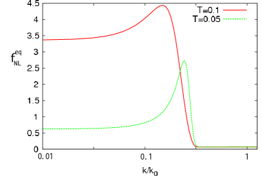
Figure 5: We plot the equilateral bispectrum for various values of $T<1$ with $d=20$. They show the featured bispectra at $k/k_{0}\simeq 0.1$.

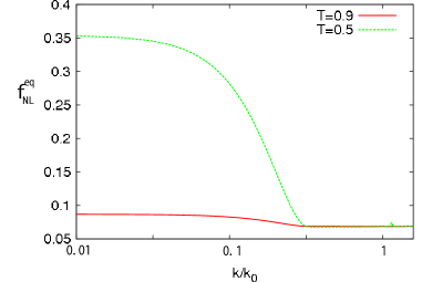
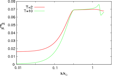
Figure 6: The equilateral bispectrum for $T<1$(left) and $T>1$(right) with $d=20$. Even though we can see small feature at subhorizon scale $k/k_{0}>1$ for large value of $T=10$, the plots generally show no detectable feature.

Next we will plot $k$-dependent nonlinear parameter $f_{NL}(k_{1},k_{2},k_{3})$. We plot a dimensionless bispectrum as a function of $x_{2}\equiv k_{2}/k_{1}$ and $x_{3}\equiv k_{3}/k_{1}$ with the free parameter $k_{1}/k_{0}$ in Fig.4. In the figure, we take $k_{1}/k_{0}=0.1$ and $k_{1}/k_{0}=1$, respectively for both same settings of $T=0.5,d=20$. Here we notice that our expansion technique is valid for $k_{1}/k_{0}\leq 1$, since we can predict the evolution only when the transition happens after the horizon crossing, $t_{k}<t_{0}$. As shown in Fig.4, for small value of $k_{1}/k_{0}<1$, the bispectrum has a peak at an equilateral shape; $k_{1}=k_{2}=k_{3}$. On the other hand, for $k_{1}/k_{0}=1$, it has a peak at a local(squeezed) shape; $k_{3}=0,k_{1}=k_{2}$.

When we focus on bispectrum for superhorizon scales, i.e., taking $k_{1}/k_{0}<{\cal O}(1)$, all bispectra have peaks at equilateral shape affected by the effect of finite changing duration time $d$, otherwise the delta approximation; $d\ll 1$ also show the local type of bispectra, which have been seen in the previous paper Park:2012rh . Our results do not depend on specifying the choice of parameter $d$, only when we consider a finite duration time; $d>{\cal O}(1)$.

Therefore, we will plot the equilateral bispectrum $f_{NL}^{eq}=f_{NL}(k_{1}=k_{2}=k_{3})$ in Fig.5, and Fig.6 for various values of $T$ with $d=20$. We can see the featured bispectrum in Fig.5 where we take small values of $T$ as $T=0.1$ and $T=0.05$, pointing $f^{eq}_{NL}={\cal O}(5)$ within the recent constraint. On the other hand, the cases for other values of $T$ show no such feature in Fig.6, where the equilateral bispectrum increases(decreases) towards super(sub)horizon scale as seen in the left(right) panel. We can also see small feature at subhorizon scale $k/k_{0}\mbox{\raisebox{-4.30554pt}{$\stackrel{{\scriptstyle\textstyle>}}{{\textstyle\sim}}$}}1$ for large value of $T=10$, however this value of amplitude of the feature is too small to be detectable.

IV Concluding remarks

We focus on the evolution of curvature perturbation on superhorizon scales by adopting the spatial gradient expansion. We have reviewed such approximation in both linear and nonlinear theory, which is called the beyond $\delta N$-formalism as the next-leading order in the expansion. In our formalism Takamizu:2010xy ; Takamizu:2013gy , we can deal with the time evolution in contrast to $\delta N$-formalism, where curvature perturbations remain just constant, and nonlinear curvature perturbation follows the simple master equation whose form is similar as one in linear theory.

As seen in (1) and (5), the evolution equation for curvature perturbation in both theories take similar structures, therefore in order to estimate the power spectrum (14) and bispectrum (21) in the approximation, all have to do is to calculating the same integrals as $D_{K}$ and $F_{k}$ in the enhancement factor: $\alpha^{\rm Lin}_{\bm{k}}$ shown in (12). It is easy to estimate non-Gaussianity, in contrast with the usual in-in formalism Maldacena:2002vr , where a numerical calculation of the correlated function would be too difficult to solve (see also Chen:2006xjb for the numerical method), if one consider a complicated situation need to solve numerically. Beyond $\delta N$-formalism takes an advantage to calculating the correlated features for power spectrum and bispectrum since the calculation is basically as same as solving the power spectrum.

As one application of our formalism for a single scalar field, we investigate the case of varying sound speed. The previous studies Khoury:2008wj ; Nakashima:2010sa ; Park:2012rh ; Emery:2012sm ; Achucarro:2012fd ; Bartolo:2013exa have done for a sudden changing, but in this paper we studied a changing with a finite duration time need to solve numerically (see Achucarro:2012fd , which also studied such mild transit in the speed of sound and also Achucarro:2013cva for recent analysis by using PLANCK data). The main purpose of this paper is to analyze whether the features can appear in the bispectrum, in particular of equilateral shape by using our nonlinear perturbation theory. The case is more suitable to calculate by using our formalism than by using the in-in formalism. We discuss local features of primordial power and bispectrum generated by the effect of varying sound speed. As shown in Takamizu:2010xy by using a similar way, we have also investigated one application of the beyond $\delta N$ for analyzing the featured bispectrum affected by a sharp change in the inflaton’s potential slope.

As shown in Fig.5, we can see a local feature like a bump at $k/k_{0}={\cal O}(0.1)$ for a small value of $T=c_{s1}/c_{s2}<{\cal O}(0.1)$ in the equilateral bispectrum, which has a peak value of non-Gaussianity; $f_{NL}^{eq}={\cal O}(10)$ at most, consistent within the recent observational constraint by PLANCK. However, such parameters also lead to the features in the power spectrum, which are excluded from the observations since the current CMB experiment gives a strong constraint, which is sensitive to $|T-1|\mbox{\raisebox{-4.30554pt}{$\stackrel{{\scriptstyle\textstyle>}}{{\textstyle\sim}}$}}0.1$ by CMB temperature power spectrum (see Nakashima:2010sa ).

This study is one toy model as a first step to investigate more realistic situation, that is for example, including a background evolution, extending to multi-field system, etc. We plan to work on this and hope to discuss them in the future.

V Acknowledgments

We thank Ryo Saito for useful discussion and comments. The work is supported by a Grant-in-Aid through JSPS No.24-2236.

References

- (1) P. Ade et al. [Planck Collaboration], arXiv:1303.5062.
- (2) C. L. Bennett et al. [WMAP Collaboration], Astrophys. J. Suppl. 208, 20 (2013), arXiv:1212.5225.
- (3) D. H. Lyth and A. Liddle, Cambridge Univ. Press, Cambridge, (2009).
- (4) P. Ade et al. [Planck Collaboration], arXiv:1303.5082.
- (5) P. Ade et al. [Planck Collaboration], arXiv:1303.5084.
- (6) M. Sasaki and D. Wands, Classical and Quantum Gravity 27, 120301 (2010).
- (7) D. S. Salopek and J. R. Bond, Phys. Rev. D42, 3936 (1990).
- (8) Y. Nambu and A. Taruya, Class. Quant. Grav. 13, 705 (1996), arXiv:astro-ph/9411013.
- (9) M. Sasaki and T. Tanaka, Prog. Theor. Phys. 99, 763 (1998), arXiv:gr-qc/9801017.
- (10) D. Wands, K. A. Malik, D. H. Lyth, and A. R. Liddle, Phys. Rev. D62, 043527 (2000), arXiv:astro-ph/0003278.
- (11) G. I. Rigopoulos and E. P. S. Shellard, Phys. Rev. D 68, 123518 (2003), arXiv:astro-ph/0306620.
- (12) D. H. Lyth and Y. Rodriguez, Phys. Rev. Lett. 95, 121302 (2005), arXiv:astro-ph/0504045.
- (13) Y. Tanaka and M. Sasaki, Prog. Theor. Phys. 117, 633 (2007), arXiv:gr-qc/0612191.
- (14) Y. Tanaka and M. Sasaki, Prog. Theor. Phys. 118, 455 (2007), arXiv:0706.0678.
- (15) Y. Takamizu and S. Mukohyama, JCAP 0901, 013 (2009), arXiv:0810.0746.
- (16) Y. Takamizu, S. Mukohyama, M. Sasaki, and Y. Tanaka, JCAP 1006, 019 (2010), arXiv:1004.1870.
- (17) Y. Takamizu and J. Yokoyama, Phys.Rev. D83, 043504 (2011), arXiv:1011.4566.
- (18) A. Naruko, Y. Takamizu and M. Sasaki, PTEP 2013, 043E01 (2013), arXiv:1210.6525.
- (19) Y. Takamizu and T. Kobayashi, PTEP 2013, no. 6, 063E03 (2013), arXiv:1301.2370.
- (20) J. M. Maldacena, JHEP 0305, 013 (2003), arXiv:astro-ph/0210603.
- (21) K. A. Malik and D. Wands, Class. Quant. Grav. 21, L65 (2004), arXiv:astro-ph/0307055.
- (22) J. Khoury and F. Piazza, JCAP 0907, 026 (2009), arXiv:0811.3633.
- (23) M. Nakashima, R. Saito, Y. Takamizu and J. Yokoyama, Prog. Theor. Phys. 125, 1035 (2011), arXiv:1009.4394.
- (24) M. Park and L. Sorbo, Phys. Rev. D 85, 083520 (2012), arXiv:1201.2903.
- (25) R. H. Ribeiro, JCAP 1205, 037 (2012), arXiv:1202.4453.
- (26) J. Emery, G. Tasinato and D. Wands, JCAP 1208, 005 (2012), arXiv:1203.6625.
- (27) A. Achucarro, J. Gong, G. A. Palma and S. P. Patil, Phys. Rev. D 87, 121301 (2013), arXiv:1211.5619.
- (28) N. Bartolo, D. Cannone and S. Matarrese, JCAP 1310, 038 (2013), arXiv:1307.3483.
- (29) A. Achucarro, V. Atal, P. Ortiz and J. Torrado, arXiv:1311.2552.
- (30) A. Achucarro, J. Gong, S. Hardeman, G. A. Palma and S. P. Patil, JCAP 1101, 030 (2011), arXiv:1010.3693.
- (31) R. Saito, M. Nakashima, Y. Takamizu and J. Yokoyama, JCAP 1211, 036 (2012), arXiv:1206.2164.
- (32) R. Saito and Y. Takamizu, JCAP 1306, 031 (2013), arXiv:1303.3839.
- (33) T. Moroi and T. Takahashi, Phys. Lett. B 522, 215 (2001), hep-ph/0110096.
- (34) D. H. Lyth and D. Wands, Phys. Lett. B 524, 5 (2002), hep-ph/0110002.
- (35) A. J. Christopherson and K. A. Malik, Phys. Lett. B 675, 159 (2009), arXiv:0809.3518.
- (36) X. Chen, R. Easther and E. A. Lim, JCAP 0706, 023 (2007), astro-ph/0611645.