An estimation of local bulk flow with the maximum-likelihood method

Abstract

A maximum-likelihood method, tested as an unbiased estimator from numerical simulations, is used to estimate cosmic bulk flow from peculiar velocity surveys. The likelihood function is applied to four observational catalogues (ENEAR, SFI++, A1SN and SC) constructed from galaxy peculiar velocity surveys and Type-Ia supernovae data at low redshift ($z\leq 0.03$). We find that the Spiral Field I-band catalogue constrains the bulk flow to be $V=290\pm 30\,{\rm km}\,{\rm s}^{-1}$ towards $l=281^{\circ}\pm 7^{\circ}$, $b=8^{\circ+6^{\circ}}_{-5^{\circ}}$ on effective scales of $58\,{h^{-1}{\rm Mpc}}$, which is the tightest constraints achievable at the present time. By comparing the amplitudes of our estimated bulk flows with theoretical prediction, we find excellent agreement between the two. In addition, directions of estimated bulk flows are also consistent with measurements in other studies.

Key words: methods: data analysis – methods: statistical – galaxies: kinematic and dynamics – cosmology: observations – large-scale structure of Universe

1 Introduction

Cosmic bulk flow is the coherent motion of galaxies and galaxy clusters towards a particular direction. Since magnitude and direction of bulk flow are determined by the underlying density field at large scales, it serves as a direct probe of the large-scale structure of the Universe. There have been a lot of recent studies focusing on estimating bulk flow from a variety of observational probes, such as galaxy peculiar velocity survey (, 2007, 2007, 2009, 2010, 2011), Type Ia supernovae data (, 2010, 2011, 2012) and galaxy clusters with observations of the cosmic microwave background (CMB) radiation (, 2010, 2011). However, amplitudes and directions of bulk flows at different depths in our local Universe obtained from different measurements do not reach good convergence. Some works have argued that the amplitude of the bulk flows they found is too high compared to the standard $\Lambda$ cold dark matter ($\Lambda$CDM) predictions (, 2009, 2010, 2010, 2011, 2012), which has stimulated a lot of interest in looking for possible explanation in new physics (, 2009, 2009, 2011).

However, any analysis which claims to strongly rule out the simple inflationary $\Lambda$CDM model should be subject to careful examination, since a confirmed large-scale flow would have profound impact on our understanding of the large-scale structure of the Universe. (2009) and (2010) adopted the minimal variance weighting method to estimate bulk flows from their combined galaxy catalogues, declaring discovery of an excess power of flow $V=407\pm 81\,{\rm km}\,{\rm s}^{-1}$ towards $l=287^{\circ}\pm 9^{\circ}$, $b=8^{\circ}\pm 6^{\circ}$ on a Gaussian window of $50\,{h^{-1}{\rm Mpc}}$ (corresponds to a top-hat window function of $\sim 100\,{h^{-1}{\rm Mpc}}$). But, by correcting Malmquist bias, selecting high-quality samples, and combining different data sets with the Bayesian hyper-parameter method, (2013) found that there is no real excess power of flow on $50\,{h^{-1}{\rm Mpc}}$ ($V\sim 310\,{\rm km}\,{\rm s}^{-1}$, $l=280^{\circ}\pm 8^{\circ}$, $b=5^{\circ}.1\pm 6^{\circ}$), and the estimated amplitude of density fluctuation $\sigma_{8}=0.65^{+0.47}_{-0.35}(\pm 1\sigma)$ is consistent with Wilkinson Microwave Anisotropy Probe (WMAP) 7-yr results (, 2011). In (2013), the minimal variance method is extended to include bulk flows in shells at different distances ($20$–$100\,{h^{-1}{\rm Mpc}}$) and a likelihood function is formulated to combine all of these reconstructed shell velocities, the multishell likelihood method yields constraints on cosmological parameters of $\sigma_{8}=1.01^{+0.26}_{-0.20}$ and $\Omega_{\rm{m}}=0.31^{+0.28}_{-0.14}$ (based on the Spiral Field I-band catalogue, in abbreviation SFI++), which are consistent with WMAP 7-yr results very well (, 2011). The recent estimation of bulk flow based on the ‘First Amendment’ compilation of 245 Type Ia supernovae found that bulk flow in the nearby Universe (a Gaussian window of $58\,{h^{-1}{\rm Mpc}}$) is of $249\pm 76\,{\rm km}\,{\rm s}^{-1}$ in the direction $l=319^{\circ}\pm 18^{\circ}$, $b=7^{\circ}\pm 14^{\circ}$ (, 2012), which is in good agreement with the expectation for the $\Lambda$CDM model ($V\sim 250\,{\rm km}\,{\rm s}^{-1}$).

Although the detailed analysis with the minimal variance and multishell likelihood methods in (2013) is in itself already a strong support to disperse the suspicion of a very large local bulk flow, it is still worthwhile to apply a different method to the same set of catalogues to check the robustness and reliability of the reconstructed bulk flow, and test the consistency between different methods. In this paper, we will use a different bulk flow reconstruction method, aka the maximum-likelihood method to calculate the bulk flows of several peculiar velocity catalogues. Furthermore, we will compare the reconstructed flows with the theoretical prediction for the $\Lambda$CDM cosmology model and investigate the tendency of the cosmic flow as a function of sample depths with currently available peculiar velocity catalogues.

This paper is organized as follows. Theoretical prediction of bulk flow on various depths $R$ and the maximum-likelihood method are presented in section 2. Introduction to the peculiar velocity samples and Malmquist bias correction is in section 3, together with specification on calculating effective depth of a sample from the geometry of the peculiar velocity survey. Section 4 shows the results of the constraints on the cosmic bulk flows by applying the likelihood function to the velocity catalogues, and the comparison against theoretical predictions. Our conclusion is in the last section.

Throughout the paper, we assume a spatially flat cosmology with WMAP 7-yr best-fitting parameter values (, 2011), i.e. fractional matter density $\Omega_{\rm m}=0.2735$, fractional baryon density $\Omega_{\rm b}=0.0455$, Hubble constant $h=0.704$, power-law index of scalar power spectrum $n_{\rm s}=0.967$ and amplitude of fluctuation $\sigma_{8}=0.811$.

2 Bulk flow model

2.1 Theoretical prediction

In the linear theory of structure formation, the velocity field $\mathbf{v}(\mathbf{r},t)$ is related to the underlying density field by (1993)

$$\mathbf{v}(\mathbf{r,}t)=\frac{f(t)H(t)}{4\pi}\int_{\rm{all\text{ }space}}\,{\rm d}^{3}\mathbf{r^{\prime}}\delta_{\rm m}(\mathbf{r^{\prime},}t)\frac{\mathbf{r}-\mathbf{r^{\prime}}}{|\mathbf{r}-\mathbf{r^{\prime}}|^{3}}\ ,$$ (1)

where $\delta_{\rm m}(\mathbf{r})=(\rho(\mathbf{r})-\overline{\rho})/\overline{\rho}$ is the density contrast at position $\mathbf{r}$, $f(t)=d\log D(t)/d\log a(t)\simeq\Omega^{4/7}_{\rm m}+(1+\Omega_{\rm m}/2)\Omega_{\Lambda}/70$ is the logrithmic derivative of the linear growth rate (Lahav et al., 1991; , 2003) and $H(t)$ is the Hubble parameter. Since the bulk flow we investigate is the streaming motion of very nearby objects, and the samples are within distance of $150\,{h^{-1}{\rm Mpc}}$ of our local volume, we take the cosmic time ‘$t$’ in Eq. (1) to be our present time $t_{0}$, thus the Hubble parameter becomes Hubble constant $H_{0}$ at $a=1$. The bulk flow $\mathbf{V}$ is the coherent motion of observed galaxies or galaxy clusters. Mathematically, $V$ is the velocity field filtered by the window function defined by the geometry of the observational sample, and is actually determined by mass distribution outside the sample space (, 1990; Nusser & Davis, 1994; Li et al., 2012). The root-mean-square(hereafter rms) of the bulk motion ($V_{\rm{rms}}$) on scale of $R$ is the velocity power spectrum filtered by the observational window function (Coles & Lucchine, 2002)

$$V_{\rm{rms}}^{2}(R) = \langle|\mathbf{V}(\mathbf{r},t_{0},R)|^{2}\rangle$$ (2)

$$= \frac{1}{(2\pi)^{3}}\int P_{\rm vv}(k)W^{2}(kR)\,{\rm d}^{3}k\ ,$$

where the $W(kR)$ is the Fourier transform of the real space selection function with size $R$. In linear regime, the velocity power spectrum at present epoch $a=1$ is (, 2007)

$$P_{\rm vv}=\frac{(H_{0}f(t_{0}))^{2}}{k^{2}}P(k)\ ,$$ (3)

where the $P(k)$ is the linear matter power spectrum which in our calculation is generated by the software package camb (, 2000). Substituting Eq. (3) into Eq. (2) and adopting the simple top-hat window function $W(x)=3(\sin x-x\cos x)/x^{3}=3j_{1}(x)/x$ (where $j_{1}(x)$ is the first spherical Bessel function), the rms of bulk velocity in a spherical region $R$ becomes (see also (2012) for derivation)

$$V_{\rm{rms}}^{2}(R) = \frac{(Hf_{0})^{2}}{(2\pi)^{3}}\int W^{2}(kR)\frac{P(k)}{k^{2}}\,{\rm d}^{3}k$$ (4)

$$= \frac{(3Hf_{0})^{2}}{2\pi^{2}}\int P(k)\left(\frac{j_{1}(kR)}{kR}\right)^{2}\,{\rm d}k\ .$$

Equation (4) is the filtered velocity power spectrum in real space, which retains large-scale modes of perturbations. The bulk velocity rms of wider window is smaller than the one for narrower size window, because more modes are smeared out. Typical rms of bulk velocity $V_{\rm{rms}}$ in $\Lambda$CDM model from top-hat window at $20\,{h^{-1}{\rm Mpc}}$ is $\sim 350\,{\rm km}\,{\rm s}^{-1}$, while at $60\,{h^{-1}{\rm Mpc}}$ is $\sim 240\,{\rm km}\,{\rm s}^{-1}$.

Now, given the filtered velocity rms on scale of $R$ (Eq. (4)), what is the probability distribution of the bulk flow magnitude on this scale? To address this question, we start from the 3D probability function of the bulk flow velocities in Cartesian coordinate. The Cartesian components of bulk flow should be Gaussian distributed, with zero means and variances of $V_{{\rm rms},x},V_{{\rm rms},y},V_{{\rm rms},z}$ respectively, assuming null correlation between the three components, the probability distribution function of bulk flow $\mathbf{V}$ is

$$p(\mathbf{V}) = p(V_{x},V_{y},V_{z})$$ (5)

$$\propto \exp\left[-\frac{1}{2}\left(\sum_{i=x,y,z}\left(\frac{V_{i}}{V_{\textrm{rms},i}}\right)^{2}\right)\right].$$

In an isotropic and homogeneous universe, the velocity field possesses the property of $V_{{\rm rms},x}^{2}=V_{{\rm rms},y}^{2}=V_{{\rm rms},z}^{2}=V_{\rm{rms}}^{2}/3$, therefore the probability of bulk flow with magnitude $V$ becomes (Bahcall et al., 1994; Coles & Lucchine, 2002)

$$p(V)\,{\rm d}V =\int\left[p(\mathbf{V})d\Omega_{V}\right]V^{2}\,{\rm d}V$$ (6)

$$= \sqrt{\frac{54}{\pi}}\left(\frac{V}{V_{\rm{rms}}}\right)^{2}\exp\left[-\frac{3}{2}\left(\frac{V}{V_{\rm{rms}}}\right)^{2}\right]\left(\frac{\,{\rm d}V}{V_{\rm{rms}}}\right),$$

where the final line of equation is properly normalized. So the amplitude of the bulk flow actually follows the Maxwell-Boltzmann distribution, which is skewed and has long tail on the large velocity branch. The peak of the distribution is $V_{\rm p}=\sqrt{2/3}V_{\rm{rms}}$, which is obtained by taking $\,{\rm d}p(V)/\,{\rm d}V=0$. One can also calculate the asymmetric variance of velocities on different depths (Li et al., 2012).

In Fig. 4, we plot the peak and $\pm 1\sigma$ variance of the bulk velocity magnitude as a function of scale $R$ in solid line and dashed lines respectively. One can clearly see that the bulk motion amplitude decreases with increasing $R$. This is because for the top-hat window function $W(x)\simeq 1$ if $x\ll 1$, but $W(x)\simeq 0$ if $x>1$, the upper limit in Eq. (2) is $R^{-1}$. Therefore, a large volume (large $R$) would result in a relatively small value of bulk flow rms. In addition, the smaller the scale is, the larger the variance of the bulk flow is. This is the effect of the sample variance, because if the velocity field is filtered on a smaller scale, larger variance of this filtered velocity will be. If one averages the peculiar velocity over the whole Universe ($R\rightarrow\infty$), the average velocity should be fairly close to zero, if the primordial perturbations are adiabatic Gaussian as assumed in the concordance $\Lambda$CDM model .

We need to mention that, the model of Equations (3) and (4) for peculiar velocity and subsequent bulk flow is made under the ‘single-particle’ assumption, i.e. the galaxies do not strongly correlate with each other and therefore Maxwellian-Boltzmann distribution can be used to describe its behaviour. Since for our peculiar velocity catalogues, the data are quite sparse and not very correlated on small scales, our assumption is a good approximation . On the other hand, in the regime where gravitational clustering of the galaxies and their collisions cannot be negligible, one needs to look in to the scale dependence of the small-scale modes and then consider the correlation between small and large scales (i.e. the gravitational quasi-equilibrium distribution method (Raychaudhury & Saslaw, 1996; Ahmad et al., 2002; Leong & Saslaw, 2004; Sivakoff & Saslaw, 2005; Saslaw & Ahmad, 2010; Saslaw, 2000)). Since we are most interested in large-scale bulk flows of which the small-scale velocity dispersion is smoothed out, we will not get involved into details of gravitational clustering properties in this paper.

2.2 The maximum-likelihood method

Figure 1: A test of the likelihood function (Eqs. (7) and (8)). ($\cos(\theta)$,$\phi$) is the direction of the bulk flow ($\theta=\pi/2-b$,$\phi=l$). The description of this test is in Section 2.2.

Now, let us move on to the issue of computing the likelihood of the magnitude and direction of the bulk flow. In general, for a peculiar velocity survey with $N$ number of objects (galaxies, galaxy clusters or Type Ia supernovae), of the $n$th object we can obtain its redshift $z_{n}$, distance $r_{n}$ (utilizing the empirical relation such as Tully-Fisher relation or the Fundamental Plane method, see Section 3.1), the line of sight velocity $S_{n}$ and its measurement error $\sigma_{n}$, and the Galactic longitude and latitude $(l,b)$ $(-90^{\circ}\leq b\leq 90^{\circ},0\leq l\leq 360^{\circ})$. The line of sight component $S_{n}$ of peculiar velocity is related to redshift ($z_{n}$) and distance ($r_{n}$) as $cz_{n}=H_{0}r_{n}+S_{n}$ (Kaiser, 1988; , 2007). Given the bulk motion $\mathbf{V}$ of objects in the sample, the residual line of sight velocity of the $n$th object after subtracting out the bulk motion is $\delta S_{n}=S_{n}-\hat{r}_{n,i}V_{i}$, where $\hat{r}_{n,i}V_{i}$ is the projected component of $\mathbf{V}$ on to the direction of line of sight . After the subtraction the residual 1D velocities should have variance $\sigma_{n}^{2}+\sigma_{\ast}^{2}$, where $\sigma_{\ast}$ accounts for the 1D intrinsic dispersion at small scales and $\sigma_{n}$ is the measurement error . Finally, the likelihood for $\mathbf{V}$=($V_{x},V_{y},V_{z}$) is constructed as (Kaiser, 1988; , 2007)

$$L(\mathbf{V},\sigma_{\ast})=\prod\limits_{n=1}^{N}\frac{1}{\sqrt{\sigma_{\ast}^{2}+\sigma_{n}^{2}}}\exp\left(-\frac{1}{2}\frac{\left(S_{n}-\hat{r}_{n,i}V_{i}\right)^{2}}{\left(\sigma_{\ast}^{2}+\sigma_{n}^{2}\right)}\right)\ .$$ (7)

Then we transform Eq. (7) into the spherical coordinate system to give the joint likelihood of magnitude $V$, direction angle $\Omega_{V}(\cos\theta,\phi)$ and $\sigma_{\ast}$,

$$L(V,\Omega_{V},\sigma_{\ast})=L(\mathbf{V},\sigma_{\ast})V^{2}$$

$$=\prod_{n=1}^{N}\frac{V^{2}}{\sqrt{\sigma_{\ast}^{2}+\sigma_{n}^{2}}}\exp\left[-\frac{1}{2}\frac{1}{(\sigma_{\ast}^{2}+\sigma^{2}_{n})}\left(S_{n}-V\left((\cos b_{n}\cos l_{n})(\sin\theta\cos\phi)+(\cos b_{n}\sin l_{n})(\sin\theta\sin\phi)+(\sin b_{n})(\cos\theta)\right)\right)\right].$$ (8)

To obtain the distribution of each parameter, we marginalize over the other parameters in the likelihood function (8).

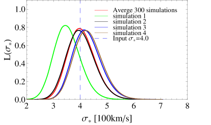
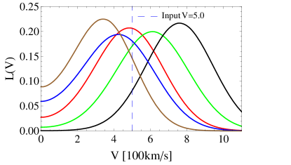
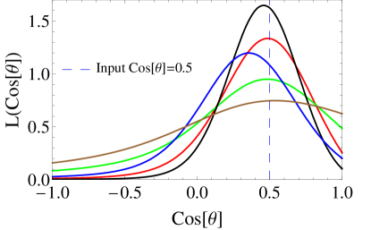
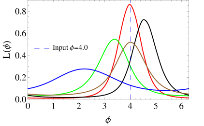
To assess performance of this likelihood function, we simulate 300 mock catalogues and test the behaviour of the likelihood with these simulated data. In each mock catalogue, we simulate 100 Type-Ia supernovae data as one data set. The way we simulate each data set is as follows. We assume that in each data set, the supernovae share a bulk flow velocity ($V=500\,{\rm km}\,{\rm s}^{-1}$) towards the direction of ($\cos(\theta)=0.5$,$\phi=4.0$) , while each line of sight velocity has $\sigma_{\ast}=400\,{\rm km}\,{\rm s}^{-1}$ random motion. We also take the measurement error of 100 samples in the “First Amendment Type-Ia Supernovae” (in abbreviation ‘A1SN’) catalogue (see Section 3.1) as the measurement errors in our simulated data sets because these quoted errors are realistic representatives of the noise of Type-Ia supernovae. Therefore, in each mock catalogue, we simulate the line of sight velocity of 100 Type-Ia supernovae samples, which share a streaming motion while each has both random error and measurement error.

We then use each mock catalogue to constrain ($V,\sigma_{\ast},\cos(\theta),\phi$) parameters, and plot the marginalized likelihood of each parameter. The constraints from four mock catalogues are demonstrated with green, black, blue and brown lines in Fig. 1. All of these distribution functions are centred around the input value of the parameters, the scattering of their peak positions is determined by the number of each sample, which scales as $1/\sqrt{N}$ with $N$ being the number of objects in the mock. In addition, the width of each distribution is determined by the measurement noise and intrinsic dispersion, as they get smaller, the width of distribution becomes narrower. We choose to simulate 100 samples in each mock catalogue is because the simulation and the maximum-likelihood analysis can be complete at relatively light expense of computing. Indeed, averaging the likelihoods of 300 mock catalogues, we find that the average distribution (red line in Fig. 1) perfectly peaks at the input values of preset parameters, which at least numerically prove that the maximum-likelihood method (Eq. (8)) can produce unbiased estimates of the bulk flow.

There are other methods designed to measure bulk flow from peculiar velocity surveys than the maximum-likelihood method. The ‘All Space Constrained Estimate’ (ASCE, 2011) is one of such methods. The method is proposed in consideration of the observational limitation that distance indicators of peculiar velocity survey, such as Tully-Fisher relation and the Fundamental Plane method, can only probe a small fraction of galaxies around our local volume ($d\lesssim 100\,{h^{-1}{\rm Mpc}}$) (, 2011). To overcome this problem, the ASCE method first generates large number of realizations of Gaussian random velocity fields based on the velocity power spectrum, these simulations are averaged to obtain a series of basis functions of bulk motion. Then they fit these basis of bulk motion with the apparent magnitude and line width of inverse Tully-Fisher relation to estimate coefficients of these basis. From these measured coefficients, one can therefore reconstruct the bulk flow in our real local Universe. (2011) confirmed the validity of this method with their mock catalogues.

Another method, proposed by Branchini et al. (2012), is to use the galaxy luminosity function at different redshifts to fit the bulk flow velocity. Redshifts of the object may be biased by the Kaiser rocket effect, Branchini et al. (2012) provides an analytical tool to correct this bias, and claims that it can lead to an unbiased reconstruction of bulk flows.

We will compare our reconstruction of the bulk flow with those found in previous studies (, 2009, 2010, 2011; Branchini et al., 2012; , 2012, 2013) in Section 4.1.

3 Peculiar velocity samples and relevant treatment

3.1 Peculiar velocity catalogues

Four different peculiar velocity catalogues from recent surveys are adopted to estimate bulk flows. The four samples are Early-type NEARby galaxies (in abbreviation ENEAR, characteristic depth $29\,{h^{-1}{\rm Mpc}}$, typical distance error $\sim 20$ per cent; 2000, 2002, 2003, 1994), SFI++ ($34\,{h^{-1}{\rm Mpc}}$,$\sim 23$ per cent; 2007), A1SN ($58\,{h^{-1}{\rm Mpc}},\sim 8$ per cent; 2007, 2009, 2010, 2012) and SC catalogue ($57\,{h^{-1}{\rm Mpc}},\sim 20$ per cent; (Giovanelli et al., 1998; Dale et al., 1999)). For details of these samples, including characteristic depths, typical distance errors and data compilation, please refer to section 3 of (2012) and section 2 of (2009).

In (2010) and (2009), there are five other catalogues employed, namely the SBF (, 2001), SN (, 2003), SMAC (, 1999, 2004), EFAR (, 2001) and Willick sample (, 1999). Here we opt to abandon these five catalogues, and the reasons are as follows. For SMAC, EFAR and Willick, these samples are either very distant, in which case the distance errors are very large, or too sparse to support robust estimation, and their survey geometry is so complicated that make it hard to measure. In addition, as the survey goes deeper, the simple model of assuming Gaussian errors of distances is almost certainly inappropriate, and will become a dominant systematic effect in the distance estimation; velocity data beyond $100\,{h^{-1}{\rm Mpc}}$ are thus too noisy to reliably reconstruct bulk flow. For SBF data, it is too close to our own galaxy, some galxies fall into our local non-linear structures, therefore it could strongly bias our estimation of bulk velocity on large scales. Since we will use the newly compiled A1SN catalogue (see 2012 and 2012) which includes three Type-Ia supernovae data sets, we will not use its old sub data set, the SN set (, 2003), in our study.

3.2 Malmquist bias correction

In the catalogues described above, there are three different classes of distance indicators, the Tully-Fisher relation (SFI++, SC), the Fundamental Plane method (ENEAR) and the Type-Ia SN luminosity function (A1SN). These distance indicators all have their intrinsic errors. For Tully-Fisher selected samples, such as SFI++ and SC, their distance errors are around $23$ per cent, which is slightly larger than the distance error of the Fundamental Plane-selected ENEAR sample ($\sim 18$ per cent). For Type-Ia supernovae data, the luminosity function can be used to calibrate the distance in better precision, the distance errors of A1SN catalogue are only $\sim 7$ per cent. The uncertainty of distance indicators, especially for Tully-Fisher and Fundamental Plane-selected objects, suggests that an object with its measured distance $d$ may actually deviate from its true distance by a broad range of possible values. This is the effect of Malmquist bias (, 1920), which characterizes the fact that inhomogeneous distribution of matter and distance (or magnitude) errors can in general bias the distance (magnitude) measurement. As a result, the probability function of the true distance $r$ given the measured distance $d$ strongly depends on the intrinsic errors of distance indicators, and the underlying density distribution (, 1920, 1988). Taking the IRAS-PSC$z$ (Point Source Catalogue with redshift) catalogue which probes the full-sky underlying density field out to $192\,{h^{-1}{\rm Mpc}}$ as the model of cosmic matter distribution, we follow the guideline in section 3.1 of (2012) and section 2.3 of (2013) to correct Malmquist bias for A1SN, SC and ENEAR catalogues. Note that the SFI++ catalogue (, 2007) is already corrected for Malmquist bias.

Once the Malmquist bias is corrected, our next step is to select samples. In the four catalogues, objects with distance beyond $100\,{h^{-1}{\rm Mpc}}$ are very sparse and suffer from large errors due to uncertainties in the distance indicators, which are consequently discarded from the sample. Additionally, several SFI++ galaxies with $d\lesssim 30\,{h^{-1}{\rm Mpc}}$ are strongly affected by local non-linear structures, showing very large velocities (, 2012), we also excluded these high-velocity members ($|v|>3000\,{\rm km}\,{\rm s}^{-1}$) from the SFI++ catalogue since they are clearly close to some local non-linear structures. Our final samples for the maximum-likelihood analysis are listed in Table 1.

catalogues	$d\leq 100$	$d>100$	$R_{\rm min}$	$R_{\rm max}$	$b_{\rm cut}$
ENEAR	$690$	$7$	$6$	$100$	$3.6$
A1SN	$175$	$100$	$5$	$100$	$0$
SFI++	$2915$	$541$	$0$	$100$	$8$
SC	$28$	$42$	$13$	$90$	$18$

Table 1: Final samples for analysis extracted from the four peculiar velocity catalogues. The first two columns give the number of galaxies within the range $d\leq 100\,{h^{-1}{\rm Mpc}}$ (used in this paper) and $d>100\,{h^{-1}{\rm Mpc}}$ (considered as outliers). The last three columns delimit geometry of samples after Malmquist bias correction and selection, $R_{\rm{min}}$ and $R_{\rm{max}}$ are the minimal and maximal distances of samples in unit of $\,{h^{-1}{\rm Mpc}}$, $|b|\leq b_{\rm{cut}}$ defines the cut-off region in galactic latitude for each survey.

3.3 Geometry of the survey

Figure 2: Upper two panels: the distance histogram of the four catalogues; lower two panels: the distribution of the ENEAR, A1SN, SFI++ and SC samples on the sky. The data are quite homogeneous across the full sky therefore robust tests of local anisotropy can be made.

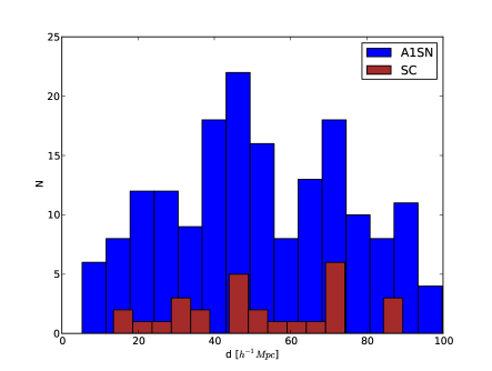
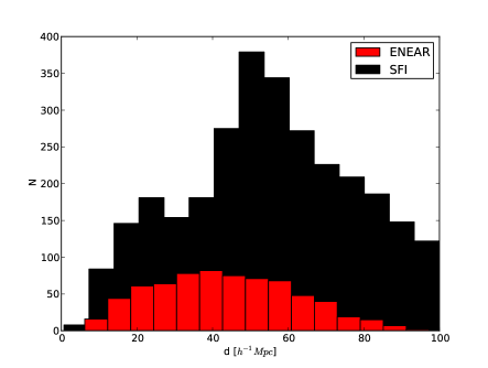
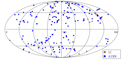
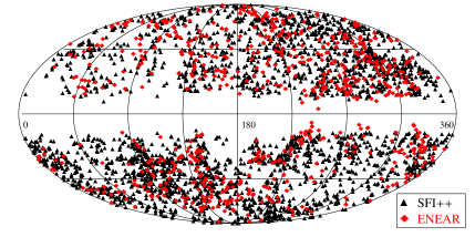
In Fig. 2 we show the histogram of the distances for each sample along the radial direction (upper two panels), and spatial distribution of the four samples on the sky (lower two panels). From the upper two panels of Fig. 2, one can see that the four samples have different distance histogram, the ENEAR catalogue is effectively the shallowest sample with the median distance around $40\,{h^{-1}{\rm Mpc}}$, while the A1SN and SFI++ catalogues all have median distance around $50\,{h^{-1}{\rm Mpc}}$. The lower two panels show that the four catalogues have nearly coverage the full sky, except for the small blank region along the galactic plane. Geometry information of the four peculiar velocity catalogues are tabulated in Table 1.

Now let us turn into the issue of calculating characteristic depth of each catalogue. The galaxy peculiar velocity survey can probe only limited depth with full or partial sky coverage. Therefore, the characteristic depth of the samples are strongly affected by this effective survey volume. (2013) and (2012) calculated the effective depth as the average of distances of all member objects. They weighted the distance of every object with the square of the inverse of its distance error, i.e.

$$\overline{r}=\frac{\sum_{n}r_{n}/\sigma^{2}_{n}}{\sum_{n}1/\sigma^{2}_{n}}\ .$$ (9)

However, the weighted-average distance does not take into account the radial distribution of the survey, as well as the influence of partial sky coverage. In this work, we adopt an alternative approach for the characteristic depth calculation proposed by Li et al. (2012) to take care of these effects. Considering the real survey geometry (Table 1) and the radial distribution function, we identify that the ‘true’ survey window function is $W_{\rm{true}}(\mathbf{x})=W(\mathbf{x})n(\mathbf{x})$, where $n(\mathbf{x})$ is the 3D density distribution. Fourier transforming the ‘true’ window function gives

$$\tilde{W}(k)=\int W_{\rm{true}}(\mathbf{x}){\rm e}^{-{\rm i}\mathbf{k}\cdot\mathbf{x}}\,{\rm d}^{3}\mathbf{x}\ ,$$ (10)

which can be plugged into Eq. (2) to yield an effective rms of bulk flow velocity (detailed calculation is in Appendix A)

$$\tilde{V}_{\rm{rms}}^{2}(R)=\frac{1}{(2\pi)^{3}}\int P_{\rm vv}(k)\tilde{W}^{2}(k)\,{\rm d}^{3}k\ .$$ (11)

The value of this velocity rms is the expectation of linear theory for the true window function. The effective depth of the sample is defined as the radius $R$ of the top-hat window function which offers the same theoretical velocity rms (Eq. (4)) as the true window function does. The effective depth is so in the sense that it filters the same modes of perturbation as the true survey window function. We list our findings of effective depth in the first column of Table 2. This characteristic depth will be used to locate the position of the bulk flow magnitude on the velocity–distance diagram (Fig. 4).

4 Results

4.1 Reconstructed bulk flow

Figure 3: Marginalized likelihood function of magnitude $V$, direction ($\cos(\theta)$,$\phi$) of the bulk flow, and the small-scale dispersion $\sigma_{\ast}$. (We marginalize Eq. (8) with respect to other parameters to obtain the likelihood of parameters of interest.) We use $\theta=\pi/2-b$,$\phi=l$, since ($\cos(\theta)$,$\phi$) are Gaussian-distributed variables. Panel (c) shows that different catalogues prefer different values of $\sigma_{\ast}$, but they all provide consistent constraints on bulk flow magnitude $V$. From panel (f), one can see that the bulk flow directions reconstructed by us are consistent with other works.

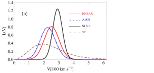
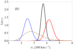
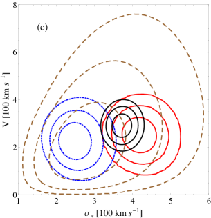
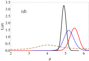
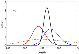
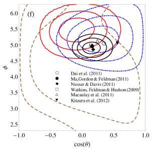
The likelihood function (Eqs. (7) and (8)) is applied for estimation of ($V$,$\cos(\theta),\phi$,$\sigma_{\ast}$) to the four peculiar velocity samples. In Fig. 3, we plot the constraints on the bulk flow $\mathbf{V}$ (panels a, d and e), the small-scale dispersion $\sigma_{\ast}$ (panel b), and joint likelihood contours on planes of ($V$,$\sigma_{\ast}$) and ($\cos(\theta)$,$\phi$) (panels c and f).

From Fig. 3a, one can see that since different surveys probe different volumes of the Universe, peaks of the likelihood functions locate at different values, reasonable comparison ought to be made together by their characteristic depths. Comparison of the constraints with the theoretical model is in Section 4.2.

In Fig. 3b, we plot the likelihood of the small-scale intrinsic velocity dispersion. It is apparent that each catalogue prefers different $\sigma_{\ast}$. For the Type-Ia supernovae sample (A1SN) and the SC catalogue, $\sigma_{\ast}$ is around $250\,{\rm km}\,{\rm s}^{-1}$, but for the SFI++ and the ENEAR, $\sigma_{\ast}$ is around $400\,{\rm km}\,{\rm s}^{-1}$. The value of $\sigma_{\ast}$ reflects the disturbance on very small scales, whilst bulk motion reflects perturbation on large scales. Thus, the bulk motion $V$ and the $\sigma_{\ast}$ should not correlate with each other, which is verified by the (nearly) orthogonal contours shown in Fig. 3c.

We further plot the likelihood of the direction angle $\cos(\theta)$ (Fig. 3e) and $\phi$ (Fig. 3d), and their correlation contours (Fig. 3f). By comparing the ($\cos(\theta)$,$\phi$) contours in Fig. 3f, with the direction angle probes by the previous studies, we can find that the direction angles constrained from our A1SN, ENEAR and SFI++ catalogues are pretty well consistent with the Type-Ia supernovae constraints by (2011), the SFI++ constraints by (2011), the combined catalogue constraints by (2009) and (2011), and the reconstructed Two-Micron All-Sky Redshift Survey density field (2012).

We list the results of our constraints in Table 2. Comparison of our results with other reconstructed bulk flow of the top-hat window function is in Table 3. In comparison, we also list the reconstructed bulk flow of Gaussian window function in Table 4.

Catalogues	$R(\,{h^{-1}{\rm Mpc}})$	$V$ ($100\,{\rm km}\,{\rm s}^{-1}$)	$\sigma_{\ast}$ ($100\,{\rm km}\,{\rm s}^{-1}$)	$l$ (∘)	$b$ (∘)
ENEAR	$49$	$2.5\pm 0.5$	$4.2\pm 0.3$	$314\pm 14$	$-6^{+11}_{-9}$
SFI++	$58$	$2.9\pm 0.3$	$3.7\pm 0.2$	$281\pm 7$	$8^{+6}_{-5}$
A1SN	$62$	$2.3\pm 0.5$	$2.5\pm 0.3$	$296\pm 16$	$15^{+13}_{-12}$
SC	$63$	$1.9^{+1.2}_{-0.9}$	$2.8^{+0.8}_{-0.6}$	$231^{\times}_{\times}$	$-2^{+35}_{-31}$

Table 2: The results of constraints from four catalogues. The $R$ is the effective top-hat window size of the sample after the Malmquist bias correct and sample selection. The error bars listed are quoted for $1\sigma$ confidence level (CL).

Samples	Numbers	$R(\,{h^{-1}{\rm Mpc}})$	$V$ ($100\,{\rm km}\,{\rm s}^{-1}$)	$l$ (∘)	$b$ (∘)	Method	References
SFI++	$2915$	$58$	$2.9\pm 0.3$	$281\pm 7$	$8^{+6}_{-5}$	MLE	This study
SFI++	$2895$	$40.0$	$3.3\pm 0.4$	$276\pm 3$	$14\pm 3$	ASCE	(2011)
SFI++	$2895$	$100.0$	$2.6\pm 0.4$	$279\pm 6$	$10\pm 6$	ASCE	(2011)
ENEAR	$690$	$49$	$2.5\pm 0.5$	$314\pm 14$	$-6^{+11}_{-9}$	MLE	This study
A1SN	$175$	$62$	$2.3\pm 0.5$	$296\pm 16$	$15^{+13}_{-12}$	MLE	This study
SN	$133$	$45.0$	$2.8\pm 0.7$	$285\pm 18$	$-10\pm 15$	MCVF	(2007)

Table 3: Comparison of the reconstructed bulk flow of the top-hat window function with the studies in the literature. The error bars listed are for $1\sigma$ CL. ‘MLE’ stands for ‘Maximum-Likelihood Estimate’; ‘ASCE’ stands for ‘All Space Constrained Estimate’; ‘MCVF’ stands for the method of extracting Multipole Components of the Velocity Field. The sample used in (2007) is the Type-Ia supernovae data from (2009) and (2007) respectively.

Samples	Numbers	$R(\,{h^{-1}{\rm Mpc}})$	$V$ ($100\,{\rm km}\,{\rm s}^{-1}$)	$l$ (∘)	$b$ (∘)	Method	References
SFI++	$2404$	$50.0$	$3.4\pm 0.4$	$280\pm 8$	$5.1\pm 6$	MV	(2013)
SFI++	$3401$	$34.0$	$4.3\pm 1.0$	N/A	N/A	MV	(2009)
ENEAR	$669$	$50.0$	$2.2\pm 0.6$	$310\pm 30$	$-9.8\pm 14$	MV	(2013)
A1SN	$153$	$50.0$	$2.2\pm 0.7$	$290\pm 60$	$12.1\pm 60$	MV	(2013)
A1SN	$245$	$58.0$	$2.5\pm 0.7$	$319\pm 18$	$7\pm 14$	MV	(2012)
SN	$557$	$150.0$	$1.9^{+1.2}_{-1.0}$	$290^{+39}_{-31}$	$20\pm 32$	MCMC	(2011)
SN	$112$	$40.0$	$5.4\pm 0.9$	$258\pm 10$	$36\pm 11$	WLS	(2011)
SN	$112$	$40.0$	$4.5\pm 1.0$	$273\pm 11$	$46\pm 8$	CU	(2011)
COMPO	$4356$	$50.0$	$4.1\pm 0.8$	$287\pm 9$	$8\pm 6$	MV	(2009)

Table 4: Comparison of the reconstructed bulk flow of the Gaussian window function with the studies in the literature. The error bars listed are for $1\sigma$ CL. ‘MLE’ stands for ‘Maximum-likelihood Estimate’; ‘MV’ stands for the ‘Minimal Variance’ method; ‘MCMC’ stands for the Bayesian Markov Chain Monte Carlo method; ‘WLS’ stands for ‘weighted least squares’; ‘CU’ stands for the ‘coefficient unbiased’ method. The sample used in (2011) is the Union2 catalogue of Type-Ia supernovae (, 2010), and the samples used in (2011) are the Type-Ia supernovae data from (2009) and (2007) respectively. The final row shows the result of COMPOSITE data set, which is a combined catalogue from eight different peculiar velocity surveys (SBF, ENEAR, SFI++, SN, SC, SMAC, EFAR, Willick).

4.2 Comparing with theoretical prediction

Figure 4: The comparison between the velocity magnitude from the likelihood function (Eq. (8)), and the theoretical evaluation (Eq. (6)) given different depths of survey.

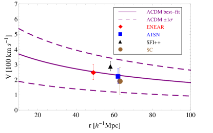
We plot our results of the constraints (Table 2) in Fig. 4 together with the predictions of the $\Lambda$CDM model. The solid line is the peak ($V_{\rm p}$) of the distribution (Eq. (6)), and the dashed lines are the $\pm 1\sigma$ confidence interval. One can see that the data are consistent with the expectation for the $\Lambda$CDM cosmology. Note that the SFI++ catalogue, with its nearly full-sky coverage and dense sampling, provides the tightest constraint of the bulk flow amplitude. In addition, by comparing our constraints with the other studies in Table 1 and the earlier works (, 1993, 1997, 2000) by using Mark III and Shallflow catalogues, we can see that they all provide constraints on bulk flow amplitude ($\sim 300\,{\rm km}\,{\rm s}^{-1}$) on scales of $50\,{h^{-1}{\rm Mpc}}$ that are consistent with the prediction for the $\Lambda$CDM model.

If the data are improved by prospective new surveys, such as 6dF survey (, 2009) or Square Kilometer Array (, ), the data can be used to constrain any possible deviation from general relativity, i.e. the standard gravity theory. This is because any alternative theory of gravity would change the growth rate of structure, which will boost or diminish the power of the velocity field on intermediate scales ($0.01\,{h{\rm Mpc}^{-1}}\lesssim k\lesssim 100\,{h{\rm Mpc}^{-1}}$) (see fig. 2 in 2012). While doing the constraints on the modified gravity model, one needs to keep in mind of the sample variance at different scales, which is plotted as the dashed line in Fig. 4. For each scale $R$, there is a certain level of uncertainty of fluctuations which reflects the variation of the number of velocity modes filtered by the window function. The sample variance limits the capacity of the reconstructed bulk flow to infer the underlying physics, one needs to consider this variance term in the full covariance matrix when the bulk flow is used to constrain cosmology.

5 Conclusion

As introduced in Section 1, bulk flow is the coherent motion of sampled galaxies, galaxy clusters or supernovae, which can be used as a test of the growth of structure. Yet there are some tentative observational evidences from the peculiar velocity surveys and the CMB observation suggesting possible excess power on scales around $50\,{h^{-1}{\rm Mpc}}$ (in radius). Here, we show that data of current peculiar velocity surveys actually do not provide strong evidence against the $\Lambda$CDM model.

In this paper we adopted a maximum-likelihood method to peculiar velocity catalogues for the bulk flow estimation. Different from just using the ‘peak’ of the maximum-likelihood method as in Kaiser (1988), we employ the full likelihood function with simulated data sets and the state-of-the-art peculiar velocity survey. Numerical test with simulations indicates that the estimator is unbiased in the limit that no complicated survey geometry is involved, which is approximately true for the four catalogues.

We apply our likelihood function to the four catalogues, ENEAR, SFI++, A1SN and SC all of which are Malmquist bias corrected and properly trimmed, to obtain the magnitude and direction of the bulk flows. We find: (1) for the largest and densest Tully-Fisher selected catalogue, SFI++ survey constrain the magnitude of bulk flow as $V=290\pm 30\,{\rm km}\,{\rm s}^{-1}$ towards $l=281^{\circ}\pm 7^{\circ}$ at an effective depth of $58\,{h^{-1}{\rm Mpc}}$, $b=8^{\circ+6^{\circ}}_{-5^{\circ}}$; (2) for the largest Fundamental Plane selected catalogue, ENEAR samples constrain the bulk flow as $V=250\pm 50\,{\rm km}\,{\rm s}^{-1}$ towards $l=314^{\circ}\pm 14^{\circ}$, $b=-6^{\circ+11^{\circ}}_{-9^{\circ}}$ at an effective depth $49\,{h^{-1}{\rm Mpc}}$. Directions of the bulk flow we find here are well consistent with the previous probes, while amplitudes of estimated bulk flows confirm an earlier investigation with the same data sets but different estimation method (, 2013).

From the geometry of the selected peculiar velocity samples, incorporating the radial distribution of sampled objects, we calculate the effective depth for the four velocity samples. Our estimated bulk speeds are placed together with the theoretical prediction of the flow at the effective depths we computed, and we find that the two matches pretty well on all scales till $50\,{h^{-1}{\rm Mpc}}$. The results of this paper clearly show that, the bulk flow velocities constrained from currently available peculiar velocity surveys do not demonstrate sign of excess large amplitudes, but rather are in full agreement with the gravitationally induced bulk flow as predicted by the concordance model of $\Lambda$CDM cosmology.

Acknowledgements: We would like to thank the discussion with Neta Bahcall, Anthony Challinor, William Saslaw, Jasper Wall and Gongbo Zhao and the two anomalous referees. YZM is supported by a CITA National Fellowship. This research is supported by the Natural Science and Engineering Research Council of Canada.

Appendix A The filtered window function

In Section 3.3, we want to take the specific survey volume into account and calculate its real window function and rms of the velocity. We identify the true survey window function as

$$W_{\rm{true}}(\mathbf{x})=W(\mathbf{x})n(\mathbf{x}),$$ (12)

where $n(\mathbf{x})=n(r,\theta,\phi)$ is the normalized density distribution

$$\int n(\mathbf{x})\,{\rm d}^{3}\mathbf{x}=1.$$ (13)

If assuming the angular distribution of samples is isotropic, the radial distribution becomes $\tilde{n}(r)=4\pi r^{2}n(r)$. But what we are interested is the “true” survey window function, by taking into account of the effective sample depth ($R_{\rm{min}}$,$R_{\rm{max}}$) and partial sky coverage ($b_{\rm{cut}}$),

$$\tilde{W}(k) = \frac{1}{\rm Vol}\int W(\mathbf{x})n(\mathbf{x})\cos(kr(\hat{\theta}\cdot\hat{\theta_{k}}))$$ (14)

$$\times r^{2}\sin(\theta)\,{\rm d}r\,{\rm d}\theta\,{\rm d}\phi,$$

where we have used the real part of the plane wave $\exp({\rm i}\mathbf{k}\cdot\mathbf{x})$ as the Fourier transform kernel. Here we express the $\mathbf{k}=(k,\theta_{k},\phi_{k})$, and Vol is the volume of the survey. Substituting the survey geometry and the cosine angle of $\theta$ and $\theta_{k}$ (i.e. $\hat{\theta}\cdot\hat{\theta_{k}}=\cos\theta\cos\theta_{k}+\sin\theta\sin\theta_{k}\cos\phi$), the radial distribution Eq. (14) becomes

$$\tilde{W}(k) = \frac{1}{4\pi\textrm{Vol}}\int^{R_{\rm{max}}}_{R_{\rm{min}}}\tilde{n}(r)$$ (15)

$$\times \cos\left(kr\left(\cos\theta\cos\theta_{k}+\sin\theta\sin\theta_{k}\cos\phi\right)\right)$$

$$\times \Theta(|\cos\theta|-\sin(b_{\rm{cut}}))\sin(\theta)\,{\rm d}r\,{\rm d}\theta\,{\rm d}\phi,$$

where $\Theta(x)$ is the Heaviside step function. The Vol in the denominator is the average factor, which ensure the $\tilde{W}(k)$ is properly normalized

Vol $$= \int W(\mathbf{x})n(\mathbf{x})\,{\rm d}^{3}x$$ (16)

$$= \left[\int^{R_{\rm{max}}}_{R_{\rm{min}}}\tilde{n}(r)\,{\rm d}r\right]$$

$$\times \left[\frac{1}{2}\int^{1}_{-1}\Theta(|\cos\theta|-\sin(b_{\rm{cut}}))\right]\,{\rm d}\cos\theta$$

$$= \left[\int^{R_{\rm{max}}}_{R_{\rm{min}}}\tilde{n}(r)\,{\rm d}r\right]\times(1-\sin(b_{\rm{cut}})).$$

Then we can substitute Eqs. (15) and (16) into Eq. (11) to calculate the rms of the bulk flow velocity $V_{\rm{rms}}$ corresponding for the true survey volume and samples.

References

- (1) Afshordi N., Geshnizjani G., & Khoury J., 2009, JCAP, 8, 30
- Ahmad et al. (2002) Ahmad F., Saslaw W. C., & Bhat N. I., 2002, ApJ, 571, 576
- (3) Amanullah R., et al., 2010, ApJ, 716, 712
- Bahcall et al. (1994) Bahcall N.A., Cen R. & Gramann M., 1994, ApJ, 430, L13
- (5) Bernardi M. et al., 2002, AJ, 123, 2990
- Branchini et al. (2012) Branchini E., Davis M., Nusser A., 2012, MNRAS, 424, 472
- Coles & Lucchine (2002) Coles P., Luccine F., Cosmology: The Origin and Evolution of Cosmic Structure, Wiley, New York, LTD, 2002
- (8) Colless M. et al., 2001, MNRAS, 321, 277
- (9) Courteau S., Faber S. M., Dressler A., Willick J. A., 1993, ApJ, 412, L51-L54
- (10) Courteau S., Willick J. A., Strauss M. A., Schlegel D, Postman M., 2000, ApJ, 544, 636
- (11) da Costa L.N. et al., 2000, AJ, 120, 95
- (12) Dai D. C., Kinney, W. H., & Stojkovic D., 2011, JCAP, 4, 15
- Dale et al. (1999) Dale D. A., Giovanelli R., Haynes M. P., Campusano L. E., Hardy E., 1999, AJ, 118, 1489
- (14) Dodelson S., Modern Cosmology (Academic Press, San Diego, 2003).
- (15) Feldman H., Watkins R., Hudson M.J., 2010, MNRAS, 407, 2328
- (16) Folatelli G. et al., 2010, AJ, 139, 120
- Giovanelli et al. (1998) Giovanelli R., Haynes M. P., Salzer J. J., Wegner G., da Costa L. N., Freudling W., 1998, AJ, 116, 2632
- (18) Haugboelle T., Hannestad S., Thomsen B., Fynbo J., Sollerman J., Jha S., 2007, ApJ, 661, 650
- (19) Hicken M. et al., 2009, ApJ, 700, 1097
- (20) Hudson M.J., 1994, MNRAS, 266, 468
- (21) Hudson M.J., 1999, PASP, 111, 57
- (22) Hudson M.J., Smith R.J., Lucey J.R., Branchini E., 2004, MNRAS, 352, 61
- (23) Jha S., Riess A.G., Kirshner R.P., 2007, ApJ, 659, 122
- (24) Jones D. H., et al., 2009, MNRAS, 399, 683
- (25) Juszkiewicz R., Vittorio N., & Wyse R. F. G., 1990, ApJ, 349, 408
- Kaiser (1988) Kaiser N., 1988, MNRAS, 231, 149
- (27) Kashlinsky A., Atrio-Barandela F., Ebeling H., Edge A., & Kocevski D., 2010, ApJ, 712, L81
- (28) Kashlinsky A., Atrio-Barandela F., Ebeling H., 2011, ApJ, 732, 1
- (29) Kitaura F.-S. et al., 2012, MNRAS, 427, 35
- (30) Komatsu E. et al., 2011, ApJS, 192, 18
- Lahav et al. (1991) Lahav, O., Lilje, P. B., Primack, J. R., & Rees, M. J. 1991, MNRAS, 251, 128
- Leong & Saslaw (2004) Leong B., & Saslaw W. C., 2004, ApJ, 608, 636
- (33) Lewis A., Challinor A., & Lasenby A., 2000, ApJ, 538, 473
- Li et al. (2012) Li M., et al., 2012, ApJ, 761, 151.
- (35) Lynden-Bell D., Faber S. M., Burstein D., Davis R. L., Dressler A., Terlevich R.J., Wegner G., 1988, ApJ, 326, 19
- (36) Ma Y. Z., Gordon C., & Feldman H. A., 2011, Phys. Rev. D, 83, 103002
- (37) Ma Y. Z., Ostriker J., & Zhao G. B., 2012a, JCAP, 06, 026
- (38) Ma Y. Z., Branchini E., & Scott D., 2012b, MNRAS, 425, 2880
- (39) Ma Y. Z., & Scott D., 2013, MNRAS, 428, 2017
- (40) Macaulay E., Feldman H., Ferreira P. G., Hudson M. J., & Watkins R., 2011, MNRAS, 414, 621
- (41) Macaulay E., Feldman H., Ferreira P. G., Jaffe A. H., Agarwal S., Hudson M. J., & Watkins R., 2012, MNRAS, 425, 1709
- (42) Malmquist K. G., 1920 Medd. Lund. Astron. Obs., Ser II, 22, 1
- (43) Mersini-Houghton L., & Holman R., 2009, JCAP, 2, 6
- Nusser & Davis (1994) Nusser, A., & Davis, M. 1994, ApJ, 421, L1
- (45) Nusser A., Davis M., 2011, ApJ, 736, 93
- (46) Peebles P. J. E., Principles of Physical Cosmology. Princeton University Press, Princeton, NJ, 1993
- Raychaudhury & Saslaw (1996) Raychaudhury S., & Saslaw W. C., 1996, ApJ, 461, 514
- (48) Sandage A., Reindl B., & Tammann G. A., 2010, ApJ, 714, 1441
- (49) Sarkar D., Feldman H.A., Watkins R., 2007, MNRAS, 375, 691
- Saslaw (2000) Saslaw W. C., 2000, The Distribution of the Galaxies: Gravitational Clustering in Cosmology, Cambridge: Cambridge Univ. Press, Cambridge
- Saslaw & Ahmad (2010) Saslaw W. C., & Ahmad F., 2010, ApJ, 720, 1246
- Sivakoff & Saslaw (2005) Sivakoff G. R., & Saslaw W. C. 2005, ApJ, 626, 795
- (53) Square Kilometre Array: http://www.skatelescope.org
- (54) Springob C.M., Masters K. L., Haynes M. P., Giovanelli R., Marinoni C., 2007, ApJS, 172, 599
- (55) Strauss M. A., Willick J. A., 1995, Phys. Rep., 261, 271
- (56) Tonry J.L. et al., 2001, ApJ, 546 681
- (57) Tonry J.L. et al., 2003, ApJ, 594, 1
- (58) Turnbull S.J., Hudson M.J., Feldman H.A., Hicken M., Kirshner R.P., Watkins R., 2012, MNRAS, 420, 447
- Turner (1991) Turner M. S., 1991, Phys. Rev. D, 44, 3737
- (60) Watkins R., Feldman H.A., Hudson M.J., 2009, MNRAS, 392, 743
- (61) Wenger G. et al., 2003, AJ, 126, 2268
- (62) Weyant A., Wood-Vasey M., Wasserman L., Freeman P., 2011, ApJ, 732, 65
- (63) Willick J. A., 1999, ApJ, 522, 647
- (64) Willick J. A., Courteau S., Faber S. M., Burstein D, Dekel A, Strauss M. A., 1997, ApJS, 109, 333