Variational approach vs accessible soliton approximation in nonlocal nonlinear media

Abstract

We discuss differences between the variational approach to solitons and the accessible soliton approximaion in a highly nonlocal nonlinear medium. We compare results of both approximations by considering the same system of equations in the same spatial region, under the same boundary conditions. We also compare these approximations with the numerical solution of the equations. We find that the variational highly nonlocal approximation provides more accurate results and as such is more appropriate solution than the accessible soliton approximation. The accessible soliton model offers a radical simplification in the treatment of highly nonlocal nonlinear media, with easy comprehension and convenient parallels to quantum harmonic oscillator, however with a hefty price tag: a systematic numerical discrepancy of up to 100% with the numerical results.

I Introduction

Self-localized wave packets which propagate in a nonlinear medium without changing their structure are known as the optical spatial solitons yuri . Their existence is a consequence of the robust balance between dispersion and nonlinearity or between diffraction and nonlinearity or between the all three in the propagation of spatiotemporal solitons or light bullets. An important characteristic of many nonlinear media is their nonlocality, i.e. the fact that the characteristic size of the response of the medium is wider than the size of the excitation itself. Strong nonlocality is of special interest, because it is observed in many media. For example, in nematic liquid crystals (NLCs) both experimental and theoretical studies demonstrated that the nonlinearity is highly nonlocal hen ; cyril ; beec .

In 1997, Snyder and Mitchell introduced a model of nonlinearity whose response is highly nonlocal snyder – in fact, infinitely nonlocal. They proposed an elegant theoretical model, intimately connected with the linear harmonic oscillator, which describes complex soliton-like dynamics (collisions, interactions, and deformations) in simple terms, even in two and three dimensions. Because of the simplicity of the theory, they coined the term ”accessible solitons” (AS) for these optical spatial solitary waves. But straightforward application of the AS theory, even in nonlinear media with almost infinite range of nonlocality, inevitably led to additional problems assanto 2003 ; assanto 2004 ; henninot , because there exists no physical medium without boundaries and without noise.

To include interactions between solitons within boundaries, as well the impact of the finite size of the sample, we developed a variational approach (VA) to solitons in nonlinear media with long-range nonlocality, such as NLCs aleksic . Starting from a convenient ansatz, this approach delivers a stationary solution for the beam amplitude and width, as well as the period of small oscillations about the stationary state. It provides for natural explanation of oscillations seen when, e.g. noise is included into the nonlocal nonlinear models. The noise is inevitable in any real physical system and causes a regular oscillation of soliton parameters with the period well predicted by our VA calculus aleksic . It may even destroy solitons petrovic . Even though our VA results were corroborated by numerics and experiments, they still attracted a volatile exchange with other researchers comment ; reply . We have further investigated the destructive influence of noise on the shape-invariant solitons in a highly nonlocal NLCs in petrovic .

In this study of VA and AS approximations to the fundamental soliton solutions in a (2+1)-dimensional highly nonlocal medium, we adopt the following model of coupled normalized equations yuri ; aleksic :

$$2i{\frac{\partial E}{\partial z}}+\Delta E+\vartheta E=0,$$ (1)

$$2\Delta\vartheta+\left|E\right|^{2}=\alpha\vartheta,$$ (2)

with zero boundary conditions on the border of a square transverse region $\left|x\right|\leq d$ and $\left|y\right|\leq d.$ Here $z$ is the propagation direction and $\Delta$ the transverse Laplacian. The system of equations of interest consists of the nonlinear Schrödinger equation for the propagation of the optical field $E$ and the diffusion equation for the nonlocal response of the medium $\vartheta$. This is a fairly general model for the nonlinear optical media with a diffusive nonlocality, widely used in the literature yuri ; assanto 2003 ; aleksic . In the local limit, the first term in Eq. (2) can be neglected and the model reduces to the Schrödinger equation with the Kerr nonlinearity. In the opposite limit, the third term in Eq. (2) can be neglected and the highly nonlocal model is reached. Since we are interested in the strong nonlocality, we will omit in our analysis the term on the right-hand side of Eq. (2).

II Variational Approach

In this approach, to derive equations describing evolution of an approximate field beam, a Lagrangian density is introduced, corresponding to equations (1, 2):

$$\mathcal{L}=i\left({\frac{\partial E^{\ast}}{\partial z}}E-{\frac{\partial E}{\partial z}}E^{\ast}\right)+\left|\nabla E\right|^{2}+\left|\nabla\vartheta\right|^{2}-\vartheta\left|E\right|^{2}.\qquad$$ (3)

Thus, the problem is reformulated into a variational problem

$$\delta\iiint\mathcal{L}dxdydz=0,$$ (4)

whose solution is equivalent to equations (1, 2). To obtain evolution equations for an approximate field in the highly nonlocal region, an ansatz is introduced in the form of a Gaussian beam for the field aleksic :

$$E=A\exp[-{\frac{r^{2}}{2R^{2}}}+iCr^{2}+i\psi],$$ (5)

in which $A$ is the amplitude, $R$ is the beam width, $C$ is the wave front curvature along the transverse coordinate, and $\psi$ is the phase shift. Variational optimization of these beam parameters will lead to the most appropriate VA solution of the problem. Likewise, a trial function for the nonlocal response of the medium is introduced, in the form

$$\vartheta=B\ \left[\textrm{Ei}(-r^{2}/T^{2})-\ln(r^{2}/d^{2})\right],$$ (6)

which is characterized by the amplitude $B$ and the width $T$. Here, Ei is the exponential integral function. Note that $T$ does not represent the total width of $\vartheta$. The form of $\vartheta$ corresponds to a radially-symmetric solution of Eq. (2), with zero boundary conditions on a circle of radius $d\gg R$ (the limit of a thick cell) abramowitz . We take this expression as an approximate solution on a square sample.

Let $\delta=\max{R^{2}/d^{2}}\ll 1$; then the averaged Lagrangian $L=\iint\mathcal{L}dxdy$ is given by:

$$\begin{split}L&=2P\psi^{\prime}+2PR^{2}\left(C^{\prime}+2C^{2}\right)+\frac{P}{R^{2}}+\\ &+4\pi B^{2}\ln\left(\frac{e^{\gamma}d^{2}}{2T^{2}}\right)-PB\ln\left(\frac{e^{\gamma}d^{2}}{R^{2}+T^{2}}\right)+O(\delta).\end{split}$$ (7)

where $\gamma$ is Euler’s constant and the prime denotes the derivative with respect to $z$. In the process of optimization from the averaged Lagrangian, one obtains four ODEs:

$$\frac{dP}{dz}=0,$$ (8)

$$C=\frac{1}{2R}\frac{dR}{dz},$$ (9)

$$\frac{d^{2}R}{dz^{2}}=\frac{1}{R^{3}}-\frac{P}{16\pi R}+O(\delta),$$ (10)

$$\frac{d\psi}{dz}=-\frac{1}{R^{2}}+\frac{P}{16\pi}\ln\left(\frac{e^{\gamma+1/2}d^{2}}{2R^{2}}\right)+O(\delta),$$ (11)

and two algebraic relations $T=R+O(\delta)$ and $B=P/8\pi+O(\delta)$. The beam power $P=\int d\varphi\int|E|^{2}rdr=\pi A^{2}R^{2}$ is conserved, according to Eq. (8). The system of equations (8-10) describes the dynamics of the beam around a stationary state.

In the stationary state $(dR/dz=dC/dz=0)$, we find the equilibrium beam width $R_{0}$ as a function of the beam power only:

$$R_{0VA}=4\sqrt{\frac{\pi}{P}}+O(\delta).$$ (12)

From relations (6, 11) we also find the maximum value of $\vartheta$:

$$\vartheta_{\max(0)}=\frac{P}{8\pi}\ln\left(\frac{e^{\gamma}}{16\pi}d^{2}P^{2}\right)+O(\delta),$$ (13)

and the propagation constant $\mu=\left(d\psi/dz\right)_{0}$ can be written as:

$$\mu=\frac{P}{16\pi}\ln\left(\frac{e^{\gamma-1/2}}{32\pi}d^{2}P^{2}\right)+O(\delta).$$ (14)

It should perhaps be mentioned that the integral quantity $\Theta=2\pi\int_{0}^{d}\vartheta rdr=P\left(d^{2}-R^{2}\right)/8+O(\delta)$ $\approx Pd^{2}/8$, which is proportional to the power, is also conserved.

The period of small oscillations of the perturbation around the equilibrium position ($R=R_{0}$, $C=C_{0}$) is given by the following relation:

$$\Lambda_{VA}=\frac{16\sqrt{2}\pi^{2}}{P}.$$ (15)

Relations (12 - 15) completely define the VA approximate solution in the highly nonlocal case. It remains to do the same for the AS approximation and then to compare the two.

III Accessible soliton approximation

In the AS approximation, the basic assumptions are that the shape of the nonlocal response of the medium is a parabolic function of the transverse distance,

$$\vartheta=\theta_{0}\ -\theta_{2}r^{2},$$ (16)

and that the shape function of the field $E$ is still a Gaussian, given by equation (5). The only refractive index ”seen” by the beam is that confined near its propagation axis snyder .

The parameters of the trial function (5) are now given by equations:

$$\frac{dA}{dz}=2AC,$$ (17)

$$C=\frac{1}{2R}\frac{dR}{dz},$$ (18)

$$\frac{d^{2}R}{dz^{2}}=\frac{1}{R^{3}}-\theta_{2}R,$$ (19)

$$\frac{d\psi}{dz}=-\frac{1}{R^{2}}+\frac{\theta_{0}}{2},$$ (20)

and equation (16), which exactly satisfy equation (1).

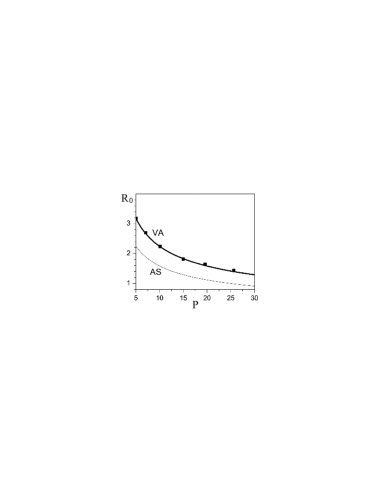
Figure 1: Stationary beam width as a function of the beam power, in both approximations. Dots represent results obtained in numerical simulations. The box width is $d=40$.

The parameter $\theta_{0}$ is only a phase shift and as such quite arbitrary. On the other hand, the value of $\theta_{2}$ is much more important; it is determined from equation (2). By replacing (5) and (16) in equation (2), in the limit $r\rightarrow 0$ one obtains $\theta_{2}=A^{2}/8$ assanto 2004 . Then, equation (19) becomes:

$$\frac{d^{2}R}{dz^{2}}=\frac{1}{R^{3}}-\frac{P}{8\pi R}.$$ (21)

The equilibrium width $R_{0}$ in the AS approximation is:

$$R_{0AS}=\sqrt{\frac{8\pi}{P}},$$ (22)

and it is $\sqrt{2}$ times less than in the VA approximation at a same power, figure 1. The corresponding stationary amplitudes in both approximations are presented in figure 2. Because of the relation $P=\pi A_{0}^{2}R_{0}^{2}$, the equilibrium amplitude $A_{0}$ in the AS approximation is $\sqrt{2}$ times greater than the one in the VA approximation at the same power.

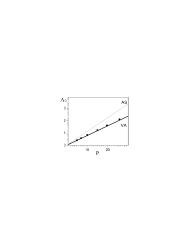
Figure 2: Stationary amplitude as a function of the beam power, in both approximations.

The period of small oscillations of the width perturbation around the equilibrium can be obtained from (21):

$$\Lambda_{AS}=\frac{8\sqrt{2}\pi^{2}}{P}.$$ (23)

The period in the AS approximation is $2$ times less than that in the VA approximation at the same power, figure 3. Thus, the values of the beam parameters for AS are systematically off the values for the VA approximation, which, on the other hand, happen to be very close to the full numerical solution for the same values of parameters.

Figure 3: Period of small oscillations as a function of the beam power, in both approximations.

Another useful approximation to AS is based on the solution of equation (2) when the parameter $\theta_{2}$ is independent of $z$. In contrast to equation (19), in which $\theta_{2}$ may depend on $z$, the equation for $R$ has an exact oscillatory solution guo

$$R=R_{0}\sqrt{\cos^{2}(\pi z/\Lambda)+\frac{P_{0}}{P}\sin^{2}(\pi z/\Lambda)},$$ (24)

from which the solutions for $C$ and $\psi$ immediately follow:

$$C=\frac{\pi}{\Lambda}\frac{\left(P_{0}/P-1\right)\sin(2\pi z/\Lambda)}{4\left(\cos^{2}(\pi z/\Lambda)+\left(P_{0}/P\right)\sin^{2}(\pi z/\Lambda)\right)},$$ (25)

$$\psi=-\arctan\left(\sqrt{P_{0}/P}\tan(\pi z/\Lambda)\right).$$ (26)

Here $R_{0}$ and $P_{0}$ are the width and the power of the AS solution, respectively. When $P=P_{0}$, one obtains stationary AS; otherwise, the approximate solution oscillates. The quantity $\Lambda=\Lambda_{AS2}\sqrt{P_{0}/P}$ represents the period of harmonic oscillations around the equilibrium (soliton) state, while $\Lambda_{AS2}$ is the period of small oscillations of the width perturbation,

$$\Lambda_{AS2}\equiv\frac{8\sqrt{2}\pi^{2}}{P}=\pi R_{0}^{2},$$ (27)

which is the same as before. Thus, in the AS approximation one obtains nice dependencies in closed form, but of little benefit, in view of the large discrepancy with the VA and the numerical solution to the full problem.

IV Conclusions

In conclusion, we have discussed the differences between the VA and AS approximate solutions to the propagation of solitons in highly nonlocal nonlinear media. The AS model provides a radical simplification and allows for an elegant description, but has a limited practical relevance, mainly because of the competition between the nonlocality and the finite size of the sample. The VA solution is not so simple, but works very well in the limited region of large nonlocality. We have found that the AS approximation can differ up to two times, when compared to the more realistic VA approximation and the numerical solution.

- (1) Kivshar Yu S and Agrawal G 2003 Optical solitons: From fibers to photonic crystals (Academic, San Diego)
- (2) Henninot J F, Blach J F and Warenghem M 2007 Experimental study of the nonlocality of spatial optical solitons excited in nematic liquid crystal J. Opt. A 9 20-25
- (3) Hutsebaut X, Cambournac C, Haelterman M, Beeckman J and Neyts K 2005 Measurement of the self-induced waveguide of a solitonlike optical beam in a nematic liquid crystal J. Opt. Soc. Am. B 22 1424-31
- (4) Beeckman J, Neyts K, Hutsebaut X, Cambournac C and Haelterman M 2004 Simulations and experiments on self-focusing conditions in nematic liquid-crystal planar cells Opt. Express 12 1011-18
- (5) Snyder A W and Mitchell D J 1997 Accessible Solitons Science 276 1538-41
- (6) Conti C, Peccianti M and Assanto G 2003 Route to Nonlocality and Observation of Accessible Solitons Phys. Rev. Lett. 91 073901
- (7) Conti C, Peccianti M and Assanto G 2004 Observation of Optical Spatial Solitons in a Highly Nonlocal Medium Phys. Rev. Lett. 92 113902
- (8) Henninot J F, Blach J F and Warenghem M 2008 The investigation of an electrically stabilized optical spatial soliton induced in a nematic liquid crystal J. Opt. A 10 085104
- (9) Aleksić N, Petrović M, Strinić A and Belić M 2012 Solitons in highly nonlocal nematic liquid crystals: Variational approach Phys. Rev. A 85 033826
- (10) Petrović M, Aleksić N, Strinić A and Belić M 2013 Destruction of shape-invariant solitons in nematic liquid crystals by noise Phys. Rev. A 87 043825
- (11) Assanto G and Smyth N 2013 Comment on ”Solitons in highly nonlocal nematic liquid crystals: Variational approach” Phys. Rev. A 87 047801
- (12) Aleksić N, Petrović M, Strinić A and Belić M 2013 Reply to ”Comment on ’Solitons in highly nonlocal nematic liquid crystals: Variational approach’ ” Phys. Rev. A 87 047802
- (13) Abramowitz M and Stegun I A 1972 Handbook of Mathematical Functions with Formulas, Graphs, and Mathematical Tables (Dover, New York)
- (14) Guo Q, Luo B, Yi F, Chi S and Xie Y 2004 Large phase shift of nonlocal optical spatial solitons Phys. Rev. E 69 016602