A Novel Family of Adaptive Filtering Algorithms Based on The Logarithmic Cost

Muhammed O. Sayin, N. Denizcan Vanli, Suleyman S. Kozat*, Senior Member, IEEE This work is in part supported by the Outstanding Researcher Programme of Turkish Academy of Sciences and TUBITAK project 112E161.The authors are with the Department of Electrical and Electronics Engineering, Bilkent University, Bilkent, Ankara 06800 Turkey, Tel: +90 (312) 290-2336, Fax: +90 (312) 290-1223 (e-mail: sayin@ee.bilkent.edu.tr, vanli@ee.bilkent.edu.tr, kozat@ee.bilkent.edu.tr).
Abstract

We introduce a novel family of adaptive filtering algorithms based on a relative logarithmic cost. The new family intrinsically combines the higher and lower order measures of the error into a single continuous update based on the error amount. We introduce important members of this family of algorithms such as the least mean logarithmic square (LMLS) and least logarithmic absolute difference (LLAD) algorithms that improve the convergence performance of the conventional algorithms. However, our approach and analysis are generic such that they cover other well-known cost functions as described in the paper. The LMLS algorithm achieves comparable convergence performance with the least mean fourth (LMF) algorithm and extends the stability bound on the step size. The LLAD and least mean square (LMS) algorithms demonstrate similar convergence performance in impulse-free noise environments while the LLAD algorithm is robust against impulsive interferences and outperforms the sign algorithm (SA). We analyze the transient, steady state and tracking performance of the introduced algorithms and demonstrate the match of the theoretical analyzes and simulation results. We show the extended stability bound of the LMLS algorithm and analyze the robustness of the LLAD algorithm against impulsive interferences. Finally, we demonstrate the performance of our algorithms in different scenarios through numerical examples.

Index Terms:
Logarithmic cost function, robustness against impulsive noise, stable adaptive method.

EDICS Category: MLR-LEAR, ASP-ANAL, MLR-APPL

I Introduction

Adaptive filtering applications such as channel equalization, noise removal or echo cancellation utilize a certain statistical measure of the error signal111Time index appears as a subscript. etsubscript𝑒𝑡e_{t} denoting the difference between the desired signal dtsubscript𝑑𝑡d_{t} and the estimation output d^tsubscript^𝑑𝑡\hat{d}_{t}. Usually, the mean square error E[et2]𝐸delimited-[]subscriptsuperscript𝑒2𝑡E[e^{2}_{t}] is used as the cost function due to its mathematical tractability and relative ease of analysis. The least mean square (LMS) and normalized least mean square (NLMS) algorithms are the members of this class [1]. In the literature, different powers of the error are commonly used as the cost function in order to provide stronger convergence or steady-state performance than the least-squares algorithms under certain settings [1].

The least mean fourth (LMF) algorithm and its family use the even powers of the error as the cost function, i.e., E[et2n]𝐸delimited-[]subscriptsuperscript𝑒2𝑛𝑡E[e^{2n}_{t}] [2]. This family achieves a better trade-off between the transient and steady-state performance, however, has stability issues [3, 4, 5]. The stability of the LMF algorithm depends on the input and noise power, and the initial value of the adaptive filter weights [6]. On the other hand, the stability of the conventional LMS algorithm depends only on the input power for a given step-size [1]. The normalized filters improve the performance of the algorithms under certain settings by removing dependency to the input statistics in the updates [7]. However, note that the normalized least mean fourth (NLMF) algorithm does not solve the stability issues [6]. In [6], authors propose the stable NLMF algorithm, which might also be derived through the proposed relative logarithmic error cost framework as shown in this paper.

The performance of the least-squares algorithms degrades severely when the input and desired signal pairs are perturbed by heavy tailed impulsive interferences, e.g., in applications involving high power noise signals [8]. In this context, we define robustness as the insensitivity of the algorithms against the impulsive interferences encountered in the practical applications and provide a theoretical framework [9]. Note that, usually, the algorithms using lower-order measures of the error in their cost function are relatively less sensitive to such perturbations. For example, the well-known sign algorithm (SA) uses the L1subscript𝐿1L_{1} norm of the error and is robust against impulsive interferences since its update involves only the sign of etsubscript𝑒𝑡e_{t}. However, the SA usually exhibits slower convergence performance especially for highly correlated input signals [10].

The mixed-norm algorithms minimize a combination of different error norms in order to achieve improved convergence performance [11, 12]. For example, [12] combines the robust L1subscript𝐿1L_{1} norm and the more sensitive but better converging L2subscript𝐿2L_{2} norm through a mixing parameter. Even though the combination parameter brings in an extra degree of freedom, the design of the mixed norm filters requires the optimization of the mixing parameter based on a priori knowledge of the input and noise statistics. On the other hand, the mixture of experts algorithms adaptively combine different algorithms and provide improved performance irrespective of the environment statistics [13, 14, 15, 16]. However, note that such mixture approaches require to operate several different algorithms on parallel, which may be infeasible in different applications [17]. In [18], authors propose an adaptive combination of L1subscript𝐿1L_{1} and L2subscript𝐿2L_{2} norms of the error in parallel, however, the resulting algorithm demonstrates impulsive perturbations on the learning curves. This results since the impulsive interferences severely degrade the algorithmic updates. In general, the samples contaminated with impulses contain little useful information [9]. Hence, the robust algorithms need to be less sensitive only against large perturbations on the error and can be as sensitive as the conventional least squares algorithms for small error values. The switched-norm algorithms switch between the L1subscript𝐿1L_{1} and L2subscript𝐿2L_{2} norms based on the error amount such as the robust Huber filter [19]. This approach combines the better convergence of L2subscript𝐿2L_{2} and the robustness of L1subscript𝐿1L_{1} together in a discrete manner with a breaking point in the cost function, however, requires optimization of certain parameters as detailed in this paper.

In this paper, we use diminishing return functions, e.g., the logarithm function, as a normalization (or a regularization) term, i.e., as a subtracting term, in the cost function in order to improve the convergence performances. We particularly choose the logarithm function as the normalizing diminishing return function [20] in our cost definitions since the logarithmic function is differentiable and results efficient and mathematically tractable adaptive algorithms. As shown in the paper, by using the logarithm function, we are able to use of the higher-order statistics of the error for small perturbations. On the other hand, for larger error values, the introduced algorithms seek to minimize the conventional cost functions due to the decreasing weight of the logarithmic term with the increasing error amount. In this sense, the new framework is akin to a continuous generalization of the switched norm algorithms, hence greatly improve the convergence performance of the mixed-norm methods as shown in this paper.

Our main contributions include: 1) We propose the least mean logarithmic square (LMLS) algorithm, which achieves a similar trade-off between the transient and steady-state performance of the LMF algorithm and as stable as the LMS algorithm; 2) We propose the least logarithmic absolute difference (LLAD) algorithm, which significantly improves the convergence performance of the SA while exhibiting comparable performance with the SA in the impulsive noise environments; 3) We analyze the transient, steady-state and tracking performance of the introduced algorithms; 4) We demonstrate the extended stability bound on the step-sizes with the logarithmic error cost framework; 5) We introduce an impulsive noise framework and analyze the robustness of the LLAD algorithm in the impulsive noise environments; 6) We demonstrate the significantly improved convergence performances of the introduced algorithms in several different scenarios in our simulations.

We organize the paper as follows. In Section II, we introduce the relative logarithmic error cost framework. In Section III, the important members of the novel family are derived. We analyze the transient, steady-state and tracking performances of those members in Section IV. In Section V, we compare the stability bound on the step-sizes and the robustness of the proposed algorithms. In Section VI, we provide the numerical examples demonstrating the improved performance of the conventional algorithms in the new logarithmic error cost framework. We conclude the paper in Section VII with several remarks.

Notation: Bold lower (or upper) case letters denote the vectors (or matrices). For a vector 𝐚𝐚\mathbf{a} (or matrix 𝐀𝐀\mathbf{A}), 𝐚Tsuperscript𝐚𝑇\mbox{$\mathbf{a}$}^{T} (or 𝐀Tsuperscript𝐀𝑇\mbox{$\mathbf{A}$}^{T}) is its ordinary transpose. \|\cdot\| and 𝐀\|\cdot\|_{\mbox{$\mathbf{A}$}} denote the L2subscript𝐿2L_{2} norm and the weighted L2subscript𝐿2L_{2} norm with the matrix 𝐀𝐀\mathbf{A}, respectively (provided that 𝐀𝐀\mathbf{A} is positive-definite). |||\cdot| is the absolute value operator. We work with real data for notational simplicity. For a random variable x𝑥x (or vector 𝐱𝐱\mathbf{x}), E[x]𝐸delimited-[]𝑥E[x] (or E[𝐱]𝐸delimited-[]𝐱E[\mbox{$\mathbf{x}$}]) represents its expectation. Here, Tr(𝐀)Tr𝐀\mathrm{Tr}(\mbox{$\mathbf{A}$}) denotes the trace of the matrix 𝐀𝐀\mathbf{A} and 𝐱f(𝐱)subscript𝐱𝑓𝐱\nabla_{\mbox{$\mathbf{x}$}}f(\mbox{$\mathbf{x}$}) is the gradient operator.

Refer to caption
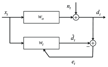
Figure 1: General system identification configuration.

II Cost Function With Logarithmic Error

We consider the system identification framework shown in Fig. 1, where we denote the input signal by 𝐱tsubscript𝐱𝑡\mbox{$\mathbf{x}$}_{t} and the desired signal by dtsubscript𝑑𝑡d_{t}. Here, we observe an unknown vector222Although we assume a time invariant unknown system vector here, we also provide the tracking performance analysis for certain non-stationary models later in the paper. 𝐰opsubscript𝐰𝑜superscript𝑝\mbox{$\mathbf{w}$}_{o}\in\mbox{$\mathbbm{R}^{p}$} through a linear model

dt=𝐰oT𝐱t+nt,subscript𝑑𝑡superscriptsubscript𝐰𝑜𝑇subscript𝐱𝑡subscript𝑛𝑡\displaystyle d_{t}=\mbox{$\mathbf{w}$}_{o}^{T}\mbox{$\mathbf{x}$}_{t}+n_{t},

where ntsubscript𝑛𝑡n_{t} represents the noise and we define the error signal as et=dtd^t=dt𝐰tT𝐱tsuperscriptsubscript𝑒𝑡subscript𝑑𝑡subscript^𝑑𝑡subscript𝑑𝑡subscriptsuperscript𝐰𝑇𝑡subscript𝐱𝑡e_{t}\stackrel{{\scriptstyle\bigtriangleup}}{{=}}d_{t}-\hat{d}_{t}=d_{t}-\mbox{$\mathbf{w}$}^{T}_{t}\mbox{$\mathbf{x}$}_{t}. In this framework, adaptive filtering algorithms estimate the unknown system vector 𝐰osubscript𝐰𝑜\mbox{$\mathbf{w}$}_{o} through the minimization of a certain cost function. The gradient descent methods usually employ convex and uni-modal cost functions in order to converge to the global minimum of the error surfaces, e.g., the mean square error E[et2]𝐸delimited-[]subscriptsuperscript𝑒2𝑡E[e^{2}_{t}] [1]. The different powers of etsubscript𝑒𝑡e_{t} [2, 10] or a linear combination of different error powers [11, 12] are also widely used.

In this framework, we use a normalized error cost function using the logarithm function given by

J(et)=F(et)1αln(1+αF(et)),superscript𝐽subscript𝑒𝑡𝐹subscript𝑒𝑡1𝛼1𝛼𝐹subscript𝑒𝑡\displaystyle J\left(e_{t}\right)\stackrel{{\scriptstyle\bigtriangleup}}{{=}}F\left(e_{t}\right)-\frac{1}{\alpha}\ln\left(1+\alpha F\left(e_{t}\right)\right), (1)

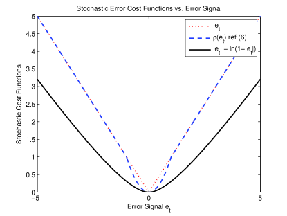
where α>0𝛼0\alpha>0 is a design parameter and F(et)𝐹subscript𝑒𝑡F\left(e_{t}\right) is a conventional cost function of the error signal etsubscript𝑒𝑡e_{t}, e.g., F(et)=E[|et|]𝐹subscript𝑒𝑡𝐸delimited-[]subscript𝑒𝑡F(e_{t})=E\left[|e_{t}|\right]. As an illustration, in Fig. 2, we compare |et|subscript𝑒𝑡|e_{t}| and |et|ln(1+|et|)subscript𝑒𝑡1subscript𝑒𝑡|e_{t}|-\ln(1+|e_{t}|). From this plot, we observe that the logarithm based cost function is less steep for small perturbations on the error while both logarithmic square and absolute difference cost functions exhibit comparable steepness for large error values. Indeed, this new family intrinsically combines the benefits of using lower and higher-order measures of the error into a single adaptation algorithm. Our algorithms provide comparable convergence rate with a conventional algorithm minimizing the cost function F(et)𝐹subscript𝑒𝑡F(e_{t}) and achieve smaller steady-state mean square errors through the use of higher-order statistics for small perturbations of the error.
Refer to caption
Figure 2: Here, we plot stochastic cost functions to illustrate decreased steepness of the least squares algorithms in the logarithmic error cost framework for small error amounts.

Remark 2.1: In [21], the authors propose a stochastic cost function using the logarithm function as follows

J[21](et)=12γln(1+γ(et𝐱t)2).superscriptsubscript𝐽[21]subscript𝑒𝑡12𝛾1𝛾superscriptsubscript𝑒𝑡normsubscript𝐱𝑡2\displaystyle J_{\mbox{\cite[cite]{[\@@bibref{}{song2013}{}{}]}}}(e_{t})\stackrel{{\scriptstyle\bigtriangleup}}{{=}}\frac{1}{2\gamma}\ln\left(1+\gamma\left(\frac{e_{t}}{\|\mbox{$\mathbf{x}$}_{t}\|}\right)^{2}\right).

Note that the cost function J[21](et)subscript𝐽[21]subscript𝑒𝑡J_{\mbox{\cite[cite]{[\@@bibref{}{song2013}{}{}]}}}(e_{t}) is the subtracted term in (1) for F(et)=et2𝐱t2𝐹subscript𝑒𝑡subscriptsuperscript𝑒2𝑡superscriptnormsubscript𝐱𝑡2F(e_{t})=\frac{e^{2}_{t}}{\|\mbox{$\mathbf{x}$}_{t}\|^{2}}. The Hessian matrix of J[21](et)subscript𝐽[21]subscript𝑒𝑡J_{\mbox{\cite[cite]{[\@@bibref{}{song2013}{}{}]}}}(e_{t}) is given by

𝐇(J[21](et))=𝐇subscript𝐽[21]subscript𝑒𝑡absent\displaystyle\mbox{$\mathbf{H}$}\left(J_{\mbox{\cite[cite]{[\@@bibref{}{song2013}{}{}]}}}(e_{t})\right)= 𝐱t𝐱tT𝐱t2(1+γ(et𝐱t)2)subscript𝐱𝑡superscriptsubscript𝐱𝑡𝑇superscriptnormsubscript𝐱𝑡21𝛾superscriptsubscript𝑒𝑡normsubscript𝐱𝑡2\displaystyle\frac{\mbox{$\mathbf{x}$}_{t}\mbox{$\mathbf{x}$}_{t}^{T}}{\|\mbox{$\mathbf{x}$}_{t}\|^{2}\left(1+\gamma\left(\frac{e_{t}}{\|\mbox{$\mathbf{x}$}_{t}\|}\right)^{2}\right)}
×(12γet2𝐱t2(1+γ(et𝐱t)2)).absent12𝛾superscriptsubscript𝑒𝑡2superscriptnormsubscript𝐱𝑡21𝛾superscriptsubscript𝑒𝑡normsubscript𝐱𝑡2\displaystyle\times\left(1-\frac{2\gamma e_{t}^{2}}{\|\mbox{$\mathbf{x}$}_{t}\|^{2}\left(1+\gamma\left(\frac{e_{t}}{\|\mbox{$\mathbf{x}$}_{t}\|}\right)^{2}\right)}\right).

We emphasize that 𝐇(J[21](et))𝐇subscript𝐽[21]subscript𝑒𝑡\mbox{$\mathbf{H}$}\left(J_{\mbox{\cite[cite]{[\@@bibref{}{song2013}{}{}]}}}(e_{t})\right) is positive semi-definite provided that γ(et𝐱t)21𝛾superscriptsubscript𝑒𝑡normsubscript𝐱𝑡21\gamma\left(\frac{e_{t}}{\|\mbox{$\mathbf{x}$}_{t}\|}\right)^{2}\leq 1, thus, the parameter γ𝛾\gamma should be chosen carefully to be able to efficiently use the gradient descent algorithms. On the other hand, we show that the new cost function in (1) is a convex function enabling the use of the diminishing return property [20] of the logarithm function for stable and robust updates.

The relative logarithmic error cost we introduce in (1) can also be expressed as

J(et)=1αln(exp(αF(et))1+αF(et)).𝐽subscript𝑒𝑡1𝛼𝛼𝐹subscript𝑒𝑡1𝛼𝐹subscript𝑒𝑡\displaystyle J(e_{t})=\frac{1}{\alpha}\ln\left(\frac{\exp\left(\alpha F(e_{t})\right)}{1+\alpha F(e_{t})}\right). (2)

Since exp(αF(et))=m=01m!αmFm(et)𝛼𝐹subscript𝑒𝑡superscriptsubscript𝑚01𝑚superscript𝛼𝑚superscript𝐹𝑚subscript𝑒𝑡\exp(\alpha F(e_{t}))=\sum_{m=0}^{\infty}\frac{1}{m!}\alpha^{m}F^{m}(e_{t}), we obtain

J(et)=1αln(1+α22!F2(et)+α33!F3(et)+1+αF(et)).𝐽subscript𝑒𝑡1𝛼1superscript𝛼22superscript𝐹2subscript𝑒𝑡superscript𝛼33superscript𝐹3subscript𝑒𝑡1𝛼𝐹subscript𝑒𝑡\displaystyle J(e_{t})=\frac{1}{\alpha}\ln\left(1+\frac{\frac{\alpha^{2}}{2!}F^{2}(e_{t})+\frac{\alpha^{3}}{3!}F^{3}(e_{t})+\cdots}{1+\alpha F(e_{t})}\right). (3)

Since F(et)𝐹subscript𝑒𝑡F(e_{t}) is a non-negative function, J(et)𝐽subscript𝑒𝑡J(e_{t}) is also a non-negative function by (3).

Remark 2.2: The Hessian matrix of J(et)𝐽subscript𝑒𝑡J(e_{t}) is given by

𝐇(J(et))=𝐇(F(et))αF(et)1+αF(et)+α𝐰F(et)𝐰F(et)T(1+αF(et))2,𝐇𝐽subscript𝑒𝑡𝐇𝐹subscript𝑒𝑡𝛼𝐹subscript𝑒𝑡1𝛼𝐹subscript𝑒𝑡𝛼subscript𝐰𝐹subscript𝑒𝑡subscript𝐰𝐹superscriptsubscript𝑒𝑡𝑇superscript1𝛼𝐹subscript𝑒𝑡2\displaystyle\mbox{$\mathbf{H}$}\left(J(e_{t})\right)=\mbox{$\mathbf{H}$}\left(F(e_{t})\right)\frac{\alpha F(e_{t})}{1+\alpha F(e_{t})}+\frac{\alpha\nabla_{\mbox{$\mathbf{w}$}}F(e_{t})\nabla_{\mbox{$\mathbf{w}$}}F(e_{t})^{T}}{\left(1+\alpha F(e_{t})\right)^{2}},

which is positive semi-definite provided that 𝐇(F(et))𝐇𝐹subscript𝑒𝑡\mbox{$\mathbf{H}$}\left(F(e_{t})\right) is a positive semi-definite matrix.

We obtain the first gradient of (1) as follows

𝐰J(et)=𝐰F(et)αF(et)1+αF(et),subscript𝐰𝐽subscript𝑒𝑡subscript𝐰𝐹subscript𝑒𝑡𝛼𝐹subscript𝑒𝑡1𝛼𝐹subscript𝑒𝑡\displaystyle\nabla_{\mbox{$\mathbf{w}$}}J(e_{t})=\nabla_{\mbox{$\mathbf{w}$}}F(e_{t})\frac{\alpha F(e_{t})}{1+\alpha F(e_{t})},

which yields zero if 𝐰F(et)subscript𝐰𝐹subscript𝑒𝑡\nabla_{\mbox{$\mathbf{w}$}}F(e_{t}) or F(et)𝐹subscript𝑒𝑡F(e_{t}) is zero. Note that the optimal solution for the cost function F(et)𝐹subscript𝑒𝑡F(e_{t}) minimizes F(et)𝐹subscript𝑒𝑡F(e_{t}) and is obtained by

𝐰=𝐰oF(et)=0.subscript𝐰subscript𝐰𝑜𝐹subscript𝑒𝑡0\displaystyle\nabla_{\mbox{$\mathbf{w}$}=\mbox{$\mathbf{w}$}_{o}}F(e_{t})=0.

Since F(et)𝐹subscript𝑒𝑡F(e_{t}) is a non-negative convex function, the global minimum and the value yielding zero gradient coincide if the latter exits. Hence, the optimal solution for the relative logarithmic error cost function is the same with the cost function F(et)𝐹subscript𝑒𝑡F(e_{t}) since as shown in Remark 2.2 the Hessian matrix of the logarithmic cost function is positive semi-definite. For example, the mean-square error cost function F(et)=E[et2]𝐹subscript𝑒𝑡𝐸delimited-[]subscriptsuperscript𝑒2𝑡F(e_{t})=E[e^{2}_{t}] yields to the Wiener solution 𝐰o=E[𝐱t𝐱tT]1E[𝐱tdt]subscript𝐰𝑜𝐸superscriptdelimited-[]subscript𝐱𝑡superscriptsubscript𝐱𝑡𝑇1𝐸delimited-[]subscript𝐱𝑡subscript𝑑𝑡\mbox{$\mathbf{w}$}_{o}=E[\mbox{$\mathbf{x}$}_{t}\mbox{$\mathbf{x}$}_{t}^{T}]^{-1}E[\mbox{$\mathbf{x}$}_{t}d_{t}].

Remark 2.3: By Maclaurin series of the natural logarithm for αF(et)1𝛼𝐹subscript𝑒𝑡1\alpha F(e_{t})\leq 1, (1) yields

J(et)𝐽subscript𝑒𝑡\displaystyle J(e_{t}) =F(et)1α(αF(et)α22F2(et)+)absent𝐹subscript𝑒𝑡1𝛼𝛼𝐹subscript𝑒𝑡superscript𝛼22superscript𝐹2subscript𝑒𝑡\displaystyle=F(e_{t})-\frac{1}{\alpha}\left(\alpha F(e_{t})-\frac{\alpha^{2}}{2}F^{2}(e_{t})+\cdots\right)
=α2F2(et)α23F3(et)+,absent𝛼2superscript𝐹2subscript𝑒𝑡superscript𝛼23superscript𝐹3subscript𝑒𝑡\displaystyle=\frac{\alpha}{2}F^{2}(e_{t})-\frac{\alpha^{2}}{3}F^{3}(e_{t})+\cdots, (4)

which is an infinite combination of the conventional cost function for small values of F(et)𝐹subscript𝑒𝑡F(e_{t}). We emphasize that the cost function (4) yields to the second power of the cost function F(et)𝐹subscript𝑒𝑡F(e_{t}) for small values of the error while for large error values, the cost function J(et)𝐽subscript𝑒𝑡J(e_{t}) resembles F(et)𝐹subscript𝑒𝑡F(e_{t}) as follows:

F(et)1αln(1+αF(et))F(et)aset.𝐹subscript𝑒𝑡1𝛼1𝛼𝐹subscript𝑒𝑡𝐹subscript𝑒𝑡assubscript𝑒𝑡\displaystyle F(e_{t})-\frac{1}{\alpha}\ln\left(1+\alpha F(e_{t})\right)\rightarrow F(e_{t})\;\mbox{as}\;e_{t}\rightarrow\infty.

Hence, the new methods are the combinations of the algorithms with mainly F2(et)superscript𝐹2subscript𝑒𝑡F^{2}(e_{t}) or F(et)𝐹subscript𝑒𝑡F(e_{t}) cost functions based on the error amount. It is important to note that the objective functions F2(et)superscript𝐹2subscript𝑒𝑡F^{2}(e_{t}), e.g., E[et2]2,𝐸superscriptdelimited-[]superscriptsubscript𝑒𝑡22E[e_{t}^{2}]^{2}, and F(et2)𝐹superscriptsubscript𝑒𝑡2F(e_{t}^{2}), e.g., E[et4],𝐸delimited-[]superscriptsubscript𝑒𝑡4E[e_{t}^{4}], yields the same stochastic gradient update after removing the expectation in this paper. The switched norm algorithms also combine two different norms into a single update in a discrete manner based on the error amount. As an example, the Huber objective function combining L1subscript𝐿1L_{1} and L2subscript𝐿2L_{2} norms of the error is defined as [19]

ρ(et)={12et2for|et|γ,γ|et|12γ2for|et|>γ,superscript𝜌subscript𝑒𝑡cases12superscriptsubscript𝑒𝑡2forsubscript𝑒𝑡𝛾𝛾subscript𝑒𝑡12superscript𝛾2forsubscript𝑒𝑡𝛾\displaystyle\rho(e_{t})\stackrel{{\scriptstyle\bigtriangleup}}{{=}}\left\{\begin{array}[]{ll}\frac{1}{2}e_{t}^{2}&\mbox{for}\;|e_{t}|\leq\gamma,\\ \gamma|e_{t}|-\frac{1}{2}\gamma^{2}&\mbox{for}\;|e_{t}|>\gamma,\end{array}\right. (7)

where γ>0𝛾0\gamma>0 denotes the cut-off value. In Fig. 2, we also compare the Huber objective function (for γ=1𝛾1\gamma=1) and the introduced cost (1) with F(et)=E[|et|]𝐹subscript𝑒𝑡𝐸delimited-[]subscript𝑒𝑡F(e_{t})=E[|e_{t}|] (for α=1𝛼1\alpha=1). Note that (7) uses a piecewise-function combining two different algorithms based on the comparison of the error with the cut-off value γ𝛾\gamma. On the other hand, logarithm based cost function J(et)𝐽subscript𝑒𝑡J(e_{t}) intrinsically combines the functions with different order of powers in a continuous manner into a single update and avoids possible anomalies that might arise due to the breaking point in the cost function.

Remark 2.4: Instead of a logarithmic normalization term, it is also possible to use various functions having diminishing returns property in order to provide stability and robustness to the conventional algorithms. For example, one can choose the cost function as

Jarctan(et)=F(et)1αarctan(αF(et))superscriptsubscript𝐽arctansubscript𝑒𝑡𝐹subscript𝑒𝑡1𝛼𝛼𝐹subscript𝑒𝑡\displaystyle J_{\mathrm{arctan}}(e_{t})\stackrel{{\scriptstyle\bigtriangleup}}{{=}}F(e_{t})-\frac{1}{\alpha}\arctan\left(\alpha F(e_{t})\right) (8)

and the Taylor series expansion of the second term in (8) around F(et)=0𝐹subscript𝑒𝑡0F(e_{t})=0 is given by

1αarctan(1+αF(et))=F(et)α23F3(et)+.1𝛼1𝛼𝐹subscript𝑒𝑡𝐹subscript𝑒𝑡superscript𝛼23superscript𝐹3subscript𝑒𝑡\displaystyle\frac{1}{\alpha}\arctan\left(1+\alpha F(e_{t})\right)=F(e_{t})-\frac{\alpha^{2}}{3}F^{3}(e_{t})+\cdots.

Thus, the resulting algorithm combines the algorithms using mainly F3(et)superscript𝐹3subscript𝑒𝑡F^{3}(e_{t}) (for small perturbations on the error) and F(et)𝐹subscript𝑒𝑡F(e_{t}). We note that the algorithms using (8) are also as stable as F(et)𝐹subscript𝑒𝑡F(e_{t}), however, they behave like minimizing the higher-order measures, i.e., F3(et)superscript𝐹3subscript𝑒𝑡F^{3}(e_{t}), for small error values.

In the next section, we propose important members of this novel adaptive filter family.

III Novel Algorithms

Based on the gradient of J(et)𝐽subscript𝑒𝑡J(e_{t}) we obtain the general steepest descent update as

𝐰t+1=𝐰tμ𝐰F(et)αF(et)1+αF(et),subscript𝐰𝑡1subscript𝐰𝑡𝜇subscript𝐰𝐹subscript𝑒𝑡𝛼𝐹subscript𝑒𝑡1𝛼𝐹subscript𝑒𝑡\displaystyle\mbox{$\mathbf{w}$}_{t+1}=\mbox{$\mathbf{w}$}_{t}-\mu\,\nabla_{\mbox{$\mathbf{w}$}}F(e_{t})\frac{\alpha F(e_{t})}{1+\alpha F(e_{t})},

where μ>0𝜇0\mu>0 is the step size and α>0𝛼0\alpha>0 is the design parameter.

Remark 3.1: In the previous section, we motivate the logarithm based error cost framework as a continuous generalization of the switched norm algorithms. The switched norm update involves a cut-off γ𝛾\gamma in the comparison of the error amount. Similarly, we utilize a design parameter α𝛼\alpha in (1) in order to determine the asymptotic cut-off value. For example, a larger α𝛼\alpha decreases the weight of the logarithmic term in the cost (1) and the resulting algorithm behaves more like minimizing the cost F(et)𝐹subscript𝑒𝑡F(e_{t}). In the performance analyzes, we show that a sufficiently small design parameter, i.e., α=1𝛼1\alpha=1, does not have determinative influence on the steady-state convergence performance under the Gaussian noise signal assumption. Hence, in the following algorithms we choose α=1𝛼1\alpha=1. On the other hand, we resort to the usage of α𝛼\alpha in order to facilitate the performance analyzes of the algorithms. Additionally, in the impulsive noise environments, we show that the optimization of α𝛼\alpha improves the steady-state convergence performance of the introduced algorithms.

If we assume that after removing the expectation to generate stochastic gradient updates F(et)𝐹subscript𝑒𝑡F(e_{t}) yields f(et)𝑓subscript𝑒𝑡f(e_{t}), e.g., F(et)=E[f(et)]𝐹subscript𝑒𝑡𝐸delimited-[]𝑓subscript𝑒𝑡F(e_{t})=E[f(e_{t})], then the general stochastic gradient update is given by

𝐰t+1subscript𝐰𝑡1\displaystyle\mbox{$\mathbf{w}$}_{t+1} =𝐰tμ𝐰etetf(et)f(et)1+f(et),absentsubscript𝐰𝑡𝜇subscript𝐰subscript𝑒𝑡subscriptsubscript𝑒𝑡𝑓subscript𝑒𝑡𝑓subscript𝑒𝑡1𝑓subscript𝑒𝑡\displaystyle=\mbox{$\mathbf{w}$}_{t}-\mu\,\nabla_{\mbox{$\mathbf{w}$}}e_{t}\nabla_{e_{t}}f(e_{t})\frac{f(e_{t})}{1+f(e_{t})},
=𝐰t+μ𝐱tetf(et)f(et)1+f(et).absentsubscript𝐰𝑡𝜇subscript𝐱𝑡subscriptsubscript𝑒𝑡𝑓subscript𝑒𝑡𝑓subscript𝑒𝑡1𝑓subscript𝑒𝑡\displaystyle=\mbox{$\mathbf{w}$}_{t}+\mu\,\mbox{$\mathbf{x}$}_{t}\nabla_{e_{t}}f(e_{t})\frac{f(e_{t})}{1+f(e_{t})}. (9)

In the following subsections, we introduce algorithms improving the performance of the conventional algorithms such as the LMS (i.e. f(et)=et2𝑓subscript𝑒𝑡subscriptsuperscript𝑒2𝑡f(e_{t})=e^{2}_{t}), sign algorithm (i.e. f(et)=|et|𝑓subscript𝑒𝑡subscript𝑒𝑡f(e_{t})=|e_{t}|) and normalized updates.

III-A The Least Mean Logarithmic Square (LMLS) Algorithm

For F(et)=E[et2]𝐹subscript𝑒𝑡𝐸delimited-[]subscriptsuperscript𝑒2𝑡F(e_{t})=E[e^{2}_{t}], the stochastic gradient update yields

𝐰t+1subscript𝐰𝑡1\displaystyle\mbox{$\mathbf{w}$}_{t+1} =𝐰t+μ𝐱tetet21+et2absentsubscript𝐰𝑡𝜇subscript𝐱𝑡subscript𝑒𝑡subscriptsuperscript𝑒2𝑡1subscriptsuperscript𝑒2𝑡\displaystyle=\mbox{$\mathbf{w}$}_{t}+\mu\mbox{$\mathbf{x}$}_{t}e_{t}\frac{e^{2}_{t}}{1+e^{2}_{t}}
=𝐰t+μ𝐱tet31+et2.absentsubscript𝐰𝑡𝜇subscript𝐱𝑡subscriptsuperscript𝑒3𝑡1subscriptsuperscript𝑒2𝑡\displaystyle=\mbox{$\mathbf{w}$}_{t}+\mu\frac{\mbox{$\mathbf{x}$}_{t}e^{3}_{t}}{1+e^{2}_{t}}. (10)

Note that we include the multiplier ‘222’ coming from the gradient etet2=2etsubscriptsubscript𝑒𝑡subscriptsuperscript𝑒2𝑡2subscript𝑒𝑡\nabla_{e_{t}}e^{2}_{t}=2e_{t} into the step-size μ𝜇\mu. The algorithm (10) resembles a least-mean fourth update for the small error values while it behaves like the least-mean square algorithm for large perturbations on the error. This provides smaller steady-state mean square error thanks to the fourth-order statistics of the error for small perturbations and stability of the least-squares algorithms for large perturbations. Hence, the LMLS algorithm intrinsically combines the least mean-square and least-mean fourth algorithms based on the error amount instead of mixed LMF + LMS algorithms [11] that need artificial combination parameter in the cost definition.

III-B The Least Logarithmic Absolute Difference (LLAD) Algorithm

The SA utilizes F(et)=E[|et|]𝐹subscript𝑒𝑡𝐸delimited-[]subscript𝑒𝑡F(e_{t})=E[|e_{t}|] as the cost function, which provides robustness against impulsive interferences [1]. However, the SA has slower convergence rate since the L1subscript𝐿1L_{1} norm is the smallest possible error power for a convex cost function. In the logarithmic cost framework, for F(et)=E[|et|]𝐹subscript𝑒𝑡𝐸delimited-[]subscript𝑒𝑡F(e_{t})=E[|e_{t}|], (9) yields

𝐰t+1subscript𝐰𝑡1\displaystyle\mbox{$\mathbf{w}$}_{t+1} =𝐰t+μ𝐱tsign(et)|et|1+|et|absentsubscript𝐰𝑡𝜇subscript𝐱𝑡signsubscript𝑒𝑡subscript𝑒𝑡1subscript𝑒𝑡\displaystyle=\mbox{$\mathbf{w}$}_{t}+\mu\mbox{$\mathbf{x}$}_{t}\mathrm{sign}(e_{t})\frac{|e_{t}|}{1+|e_{t}|}
=𝐰t+μ𝐱tet1+|et|.absentsubscript𝐰𝑡𝜇subscript𝐱𝑡subscript𝑒𝑡1subscript𝑒𝑡\displaystyle=\mbox{$\mathbf{w}$}_{t}+\mu\frac{\mbox{$\mathbf{x}$}_{t}e_{t}}{1+|e_{t}|}. (11)

The algorithm (11) combines the LMS algorithm and SA into a single robust algorithm with improved convergence performance. We note that in Section V we calculate the optimum αoptsubscript𝛼opt\alpha_{\mathrm{opt}} in order to achieve better convergence performance than the SA in the impulsive noise environments.

III-C Normalized Updates

We introduce normalized updates with respect to the regressor signal in order to provide independence from the input data correlation statistics under certain settings. We define the new objective function as

Jnew(et)=F(et𝐱t)1αln(1+αF(et𝐱t)),superscriptsubscript𝐽newsubscript𝑒𝑡𝐹subscript𝑒𝑡normsubscript𝐱𝑡1𝛼1𝛼𝐹subscript𝑒𝑡normsubscript𝐱𝑡\displaystyle J_{\mathrm{new}}(e_{t})\stackrel{{\scriptstyle\bigtriangleup}}{{=}}F\left(\frac{e_{t}}{\|\mbox{$\mathbf{x}$}_{t}\|}\right)-\frac{1}{\alpha}\ln\left(1+\alpha F\left(\frac{e_{t}}{\|\mbox{$\mathbf{x}$}_{t}\|}\right)\right),

for example F(et𝐱t)=E[et2𝐱t2]𝐹subscript𝑒𝑡normsubscript𝐱𝑡𝐸delimited-[]superscriptsubscript𝑒𝑡2superscriptnormsubscript𝐱𝑡2F\left(\frac{e_{t}}{\|\mbox{$\mathbf{x}$}_{t}\|}\right)=E\left[\frac{e_{t}^{2}}{\|\mbox{$\mathbf{x}$}_{t}\|^{2}}\right]. The Hessian matrix of the new cost function Jnew(et)subscript𝐽newsubscript𝑒𝑡J_{\mathrm{new}}(e_{t}) is also positive semi-definite provided that the Hessian matrix of F(et𝐱t)𝐹subscript𝑒𝑡normsubscript𝐱𝑡F\left(\frac{e_{t}}{\|\mbox{$\mathbf{x}$}_{t}\|}\right) is positive semi-definite as shown in Remark 2.2.

The steepest-descent update is given by

𝐰t+1=𝐰tμ𝐰F(et𝐱t)αF(et𝐱t)1+αF(et𝐱t).subscript𝐰𝑡1subscript𝐰𝑡𝜇subscript𝐰𝐹subscript𝑒𝑡normsubscript𝐱𝑡𝛼𝐹subscript𝑒𝑡normsubscript𝐱𝑡1𝛼𝐹subscript𝑒𝑡normsubscript𝐱𝑡\displaystyle\mbox{$\mathbf{w}$}_{t+1}=\mbox{$\mathbf{w}$}_{t}-\mu\nabla_{\mbox{$\mathbf{w}$}}F\left(\frac{e_{t}}{\|\mbox{$\mathbf{x}$}_{t}\|}\right)\frac{\alpha F\left(\frac{e_{t}}{\|\mbox{$\mathbf{x}$}_{t}\|}\right)}{1+\alpha F\left(\frac{e_{t}}{\|\mbox{$\mathbf{x}$}_{t}\|}\right)}.

For F(et𝐱t)=E[(et𝐱t)]2F(\frac{e_{t}}{\|\mbox{$\mathbf{x}$}_{t}\|})=E\left[\right(\frac{e_{t}}{\|\mbox{$\mathbf{x}$}_{t}\|}\left){}^{2}\right], we get the normalized least mean logarithmic square (NLMLS) algorithm given by

𝐰t+1=𝐰t+μ𝐱tet3𝐱t2(𝐱t2+et2).subscript𝐰𝑡1subscript𝐰𝑡𝜇subscript𝐱𝑡subscriptsuperscript𝑒3𝑡superscriptnormsubscript𝐱𝑡2superscriptnormsubscript𝐱𝑡2subscriptsuperscript𝑒2𝑡\displaystyle\mbox{$\mathbf{w}$}_{t+1}=\mbox{$\mathbf{w}$}_{t}+\mu\frac{\mbox{$\mathbf{x}$}_{t}e^{3}_{t}}{\|\mbox{$\mathbf{x}$}_{t}\|^{2}\left(\|\mbox{$\mathbf{x}$}_{t}\|^{2}+e^{2}_{t}\right)}. (12)

We point out that (12) is also proposed as the stable normalized least mean-fourth algorithm in [6].

For F(et𝐱t)=E[|et|𝐱t]𝐹subscript𝑒𝑡normsubscript𝐱𝑡𝐸delimited-[]subscript𝑒𝑡normsubscript𝐱𝑡F(\frac{e_{t}}{\|\mbox{$\mathbf{x}$}_{t}\|})=E\left[\frac{|e_{t}|}{\|\mbox{$\mathbf{x}$}_{t}\|}\right], we obtain the normalized least logarithmic absolute difference (NLLAD) algorithm as

𝐰t+1=𝐰t+μ𝐱tet𝐱t(𝐱t+|et|).subscript𝐰𝑡1subscript𝐰𝑡𝜇subscript𝐱𝑡subscript𝑒𝑡normsubscript𝐱𝑡normsubscript𝐱𝑡subscript𝑒𝑡\displaystyle\mbox{$\mathbf{w}$}_{t+1}=\mbox{$\mathbf{w}$}_{t}+\frac{\mu\,\mbox{$\mathbf{x}$}_{t}e_{t}}{\|\mbox{$\mathbf{x}$}_{t}\|\left(\|\mbox{$\mathbf{x}$}_{t}\|+|e_{t}|\right)}.

In the next section, we analyze the transient and steady state performance of the introduced algorithms.

IV Performance Analysis

We define a priori estimation error and the weighted form as

ea,t=𝐱tT𝐰~tandea,t𝚺=𝐱tT𝚺𝐰~t,superscriptsubscript𝑒𝑎𝑡subscriptsuperscript𝐱𝑇𝑡subscript~𝐰𝑡andsuperscriptsubscript𝑒𝑎𝑡𝚺superscriptsubscriptsuperscript𝐱𝑇𝑡𝚺subscript~𝐰𝑡\displaystyle e_{a,t}\stackrel{{\scriptstyle\bigtriangleup}}{{=}}\mbox{$\mathbf{x}$}^{T}_{t}\tilde{\mbox{$\mathbf{w}$}}_{t}\;\mbox{and}\;e_{a,t}^{\mbox{$\mathbf{\Sigma}$}}\stackrel{{\scriptstyle\bigtriangleup}}{{=}}\mbox{$\mathbf{x}$}^{T}_{t}\mbox{$\mathbf{\Sigma}$}\tilde{\mbox{$\mathbf{w}$}}_{t},

where 𝐰~t=𝐰o𝐰tsuperscriptsubscript~𝐰𝑡subscript𝐰𝑜subscript𝐰𝑡\tilde{\mbox{$\mathbf{w}$}}_{t}\stackrel{{\scriptstyle\bigtriangleup}}{{=}}\mbox{$\mathbf{w}$}_{o}-\mbox{$\mathbf{w}$}_{t} and 𝚺𝚺\mathbf{\Sigma} is a symmetric positive definite weighting matrix. Different choice of 𝚺𝚺\mathbf{\Sigma} leads to the different performance measures of the algorithm [1]. In the analyzes, we include the design parameter α𝛼\alpha in order to facilitate the theoretical analyzes. After some algebra, we obtain the weighted-energy recursion [1, 22, 23] as

E[𝐰~t+1𝚺2]𝐸delimited-[]superscriptsubscriptnormsubscript~𝐰𝑡1𝚺2\displaystyle E\left[\|\tilde{\mbox{$\mathbf{w}$}}_{t+1}\|_{\mbox{$\mathbf{\Sigma}$}}^{2}\right] =E[𝐰~t𝚺2]absent𝐸delimited-[]superscriptsubscriptnormsubscript~𝐰𝑡𝚺2\displaystyle=E\left[\|\tilde{\mbox{$\mathbf{w}$}}_{t}\|_{\mbox{$\mathbf{\Sigma}$}}^{2}\right]
μ2𝜇2\displaystyle-\mu 2 E[ea,t𝚺etf(et)αf(et)1+αf(et)]𝐸delimited-[]superscriptsubscript𝑒𝑎𝑡𝚺subscriptsubscript𝑒𝑡𝑓subscript𝑒𝑡𝛼𝑓subscript𝑒𝑡1𝛼𝑓subscript𝑒𝑡\displaystyle E\left[e_{a,t}^{\mbox{$\mathbf{\Sigma}$}}\nabla_{e_{t}}f(e_{t})\frac{\alpha f(e_{t})}{1+\alpha f(e_{t})}\right]
+μ2superscript𝜇2\displaystyle+\mu^{2} E[𝐱t𝚺2(etf(et)αf(et)1+αf(et))2].𝐸delimited-[]superscriptsubscriptnormsubscript𝐱𝑡𝚺2superscriptsubscriptsubscript𝑒𝑡𝑓subscript𝑒𝑡𝛼𝑓subscript𝑒𝑡1𝛼𝑓subscript𝑒𝑡2\displaystyle E\left[\|\mbox{$\mathbf{x}$}_{t}\|_{\mbox{$\mathbf{\Sigma}$}}^{2}\left(\nabla_{e_{t}}f(e_{t})\frac{\alpha f(e_{t})}{1+\alpha f(e_{t})}\right)^{2}\right]. (13)

For notational simplicity, we define

g(et)=etf(et)αf(et)1+αf(et).superscript𝑔subscript𝑒𝑡subscriptsubscript𝑒𝑡𝑓subscript𝑒𝑡𝛼𝑓subscript𝑒𝑡1𝛼𝑓subscript𝑒𝑡g(e_{t})\stackrel{{\scriptstyle\bigtriangleup}}{{=}}\nabla_{e_{t}}f(e_{t})\frac{\alpha f(e_{t})}{1+\alpha f(e_{t})}. (14)

Then, (13) yields the general weighted-energy recursion [23] as follows

E[𝐰~t+1𝚺2]=𝐸delimited-[]superscriptsubscriptnormsubscript~𝐰𝑡1𝚺2absent\displaystyle E\left[\|\tilde{\mbox{$\mathbf{w}$}}_{t+1}\|_{\mbox{$\mathbf{\Sigma}$}}^{2}\right]= E[𝐰~t𝚺2]μ2E[ea,t𝚺g(et)]𝐸delimited-[]superscriptsubscriptnormsubscript~𝐰𝑡𝚺2𝜇2𝐸delimited-[]superscriptsubscript𝑒𝑎𝑡𝚺𝑔subscript𝑒𝑡\displaystyle\,E\left[\|\tilde{\mbox{$\mathbf{w}$}}_{t}\|_{\mbox{$\mathbf{\Sigma}$}}^{2}\right]-\mu 2E\left[e_{a,t}^{\mbox{$\mathbf{\Sigma}$}}g(e_{t})\right]
+μ2E[𝐱t𝚺2g2(et)].superscript𝜇2𝐸delimited-[]superscriptsubscriptnormsubscript𝐱𝑡𝚺2superscript𝑔2subscript𝑒𝑡\displaystyle+\mu^{2}E\left[\|\mbox{$\mathbf{x}$}_{t}\|_{\mbox{$\mathbf{\Sigma}$}}^{2}g^{2}(e_{t})\right]. (15)

In the subsequent analysis of (13), we use the following assumptions:

Assumption 1:

The observation noise ntsubscript𝑛𝑡n_{t} is zero-mean independently and identically distributed (i.i.d.) Gaussian random variable and independent from 𝐱tsubscript𝐱𝑡\mbox{$\mathbf{x}$}_{t}. The regressor signal 𝐱tsubscript𝐱𝑡\mbox{$\mathbf{x}$}_{t} is also zero-mean i.i.d. Gaussian random variable with the auto-correlation matrix 𝐑=E[𝐱t𝐱tT]superscript𝐑𝐸delimited-[]subscript𝐱𝑡subscriptsuperscript𝐱𝑇𝑡\mbox{$\mathbf{R}$}\stackrel{{\scriptstyle\bigtriangleup}}{{=}}E\left[\mbox{$\mathbf{x}$}_{t}\mbox{$\mathbf{x}$}^{T}_{t}\right].

Assumption 2:

The estimation error etsubscript𝑒𝑡e_{t} and the noise ntsubscript𝑛𝑡n_{t} are jointly Gaussian. The Gaussian estimation error assumption is acceptable for sufficiently small step size μ𝜇\mu and through the Assumption 1 [1].

Assumption 3:

The estimation error etsubscript𝑒𝑡e_{t} is jointly Gaussian with the weighted a priori estimation error ea,t𝚺superscriptsubscript𝑒𝑎𝑡𝚺e_{a,t}^{\mbox{$\mathbf{\Sigma}$}} for any constant matrix 𝚺𝚺\mathbf{\Sigma}. The assumption is reasonable for long filters, i.e. p𝑝p is large, sufficiently small step size μ𝜇\mu [23], and by Assumption 2.

Assumption 4:

The random variables 𝐱t𝚺2superscriptsubscriptnormsubscript𝐱𝑡𝚺2\|\mbox{$\mathbf{x}$}_{t}\|_{\mbox{$\mathbf{\Sigma}$}}^{2} and g2(et)superscript𝑔2subscript𝑒𝑡g^{2}(e_{t}) are uncorrelated, which enables the following split as

E[𝐱t𝚺2g2(et)]=E[𝐱t𝚺2]E[g2(et)].𝐸delimited-[]superscriptsubscriptnormsubscript𝐱𝑡𝚺2superscript𝑔2subscript𝑒𝑡𝐸delimited-[]superscriptsubscriptnormsubscript𝐱𝑡𝚺2𝐸delimited-[]superscript𝑔2subscript𝑒𝑡\displaystyle E\left[\|\mbox{$\mathbf{x}$}_{t}\|_{\mbox{$\mathbf{\Sigma}$}}^{2}g^{2}(e_{t})\right]=E\left[\|\mbox{$\mathbf{x}$}_{t}\|_{\mbox{$\mathbf{\Sigma}$}}^{2}\right]E\left[g^{2}(e_{t})\right].

We next analyze the transient behavior of the new algorithms through the energy recursion (13).

IV-A Transient Analysis

In the following we evaluate (13) term by term. We first consider the second term in the right hand side (RHS) of (IV) and introduce the following lemma

Lemma 1: Under Assumptions 1-4, we have

E[ea,t𝚺g(et)]=E[ea,t𝚺et]E[etg(et)]E[et2].𝐸delimited-[]superscriptsubscript𝑒𝑎𝑡𝚺𝑔subscript𝑒𝑡𝐸delimited-[]superscriptsubscript𝑒𝑎𝑡𝚺subscript𝑒𝑡𝐸delimited-[]subscript𝑒𝑡𝑔subscript𝑒𝑡𝐸delimited-[]subscriptsuperscript𝑒2𝑡E[e_{a,t}^{\mbox{$\mathbf{\Sigma}$}}g(e_{t})]=E[e_{a,t}^{\mbox{$\mathbf{\Sigma}$}}e_{t}]\frac{E[e_{t}g(e_{t})]}{E[e^{2}_{t}]}. (16)

Proof: The proof of Lemma 1 follows from the Price’s result [24, 25]. That is, for any Borel function g(b)𝑔𝑏g(b) we can write

E[xg(y)]=E[xy]E[y2]E[yg(y)],𝐸delimited-[]𝑥𝑔𝑦𝐸delimited-[]𝑥𝑦𝐸delimited-[]superscript𝑦2𝐸delimited-[]𝑦𝑔𝑦\displaystyle E[xg(y)]=\frac{E[xy]}{E[y^{2}]}E[yg(y)],

where x𝑥x and y𝑦y are zero-mean jointly Gaussian random variables [26]. Hence by Assumptions 2 and 3, we obtain (16) and the proof is concluded. \square

Since et=ea,t+ntsubscript𝑒𝑡subscript𝑒𝑎𝑡subscript𝑛𝑡e_{t}=e_{a,t}+n_{t}, we obtain

E[ea,t𝚺et]=E[ea,t𝚺ea,t]=E[𝐰~t𝚺𝐱t𝐱tT2],𝐸delimited-[]superscriptsubscript𝑒𝑎𝑡𝚺subscript𝑒𝑡𝐸delimited-[]superscriptsubscript𝑒𝑎𝑡𝚺subscript𝑒𝑎𝑡𝐸delimited-[]superscriptsubscriptnormsubscript~𝐰𝑡subscript𝚺𝐱𝑡subscriptsuperscript𝐱𝑇𝑡2\displaystyle E\left[e_{a,t}^{\mbox{$\mathbf{\Sigma}$}}e_{t}\right]=E\left[e_{a,t}^{\mbox{$\mathbf{\Sigma}$}}e_{a,t}\right]=E\left[\|\tilde{\mbox{$\mathbf{w}$}}_{t}\|_{\mbox{$\mathbf{\Sigma}$}\mbox{$\mathbf{x}$}_{t}\mbox{$\mathbf{x}$}^{T}_{t}}^{2}\right], (17)

by Assumption 1. Additionally, by the independence assumption for the regressor 𝐱tsubscript𝐱𝑡\mbox{$\mathbf{x}$}_{t} (i.e., Assumptions 1 and 4), we can simplify the third term in the RHS of (IV). Hence, the weighted-error recursion (IV) could be written as follows [23]

E[𝐰~t+1𝚺2]=𝐸delimited-[]superscriptsubscriptnormsubscript~𝐰𝑡1𝚺2absent\displaystyle E\left[\|\tilde{\mbox{$\mathbf{w}$}}_{t+1}\|_{\mbox{$\mathbf{\Sigma}$}}^{2}\right]=\, E[𝐰~t𝚺2]μ2hG(et)E[𝐰~t𝚺𝐑2]𝐸delimited-[]superscriptsubscriptnormsubscript~𝐰𝑡𝚺2𝜇2subscript𝐺subscript𝑒𝑡𝐸delimited-[]superscriptsubscriptnormsubscript~𝐰𝑡𝚺𝐑2\displaystyle E\left[\|\tilde{\mbox{$\mathbf{w}$}}_{t}\|_{\mbox{$\mathbf{\Sigma}$}}^{2}\right]-\mu 2h_{G}\left(e_{t}\right)E\left[\|\tilde{\mbox{$\mathbf{w}$}}_{t}\|_{\mbox{$\mathbf{\Sigma}$}\mbox{$\mathbf{R}$}}^{2}\right]
+μ2E[𝐱t𝚺2]hU(et),superscript𝜇2𝐸delimited-[]superscriptsubscriptnormsubscript𝐱𝑡𝚺2subscript𝑈subscript𝑒𝑡\displaystyle+\mu^{2}E\left[\|\mbox{$\mathbf{x}$}_{t}\|_{\mbox{$\mathbf{\Sigma}$}}^{2}\right]h_{U}\left(e_{t}\right), (18)

where

hG(et)=E[etg(et)]E[et2],hU(et)=E[g2(et)].formulae-sequencesuperscriptsubscript𝐺subscript𝑒𝑡𝐸delimited-[]subscript𝑒𝑡𝑔subscript𝑒𝑡𝐸delimited-[]subscriptsuperscript𝑒2𝑡superscriptsubscript𝑈subscript𝑒𝑡𝐸delimited-[]superscript𝑔2subscript𝑒𝑡\displaystyle h_{G}(e_{t})\stackrel{{\scriptstyle\bigtriangleup}}{{=}}\frac{E[e_{t}g(e_{t})]}{E[e^{2}_{t}]},\;\;h_{U}(e_{t})\stackrel{{\scriptstyle\bigtriangleup}}{{=}}E\left[g^{2}(e_{t})\right].
TABLE I: hG(et)subscript𝐺subscript𝑒𝑡h_{G}(e_{t}) and hU(et)subscript𝑈subscript𝑒𝑡h_{U}(e_{t}) corresponding to the stochastic costs et2subscriptsuperscript𝑒2𝑡e^{2}_{t} and |et|subscript𝑒𝑡|e_{t}|, where σe2=E[et2]superscriptsubscript𝜎𝑒2𝐸delimited-[]subscriptsuperscript𝑒2𝑡\sigma_{e}^{2}=E[e^{2}_{t}] and λ=12ασe2=ακ𝜆12𝛼superscriptsubscript𝜎𝑒2𝛼𝜅\lambda=\frac{1}{2\alpha\sigma_{e}^{2}}=\alpha\kappa.
Algorithm hG(et)subscript𝐺subscript𝑒𝑡h_{G}(e_{t}) hU(et)subscript𝑈subscript𝑒𝑡h_{U}(e_{t})
LMF 3σe23superscriptsubscript𝜎𝑒23\sigma_{e}^{2} 15σe615superscriptsubscript𝜎𝑒615\sigma_{e}^{6}
LMLS 12λ(1πλexp(λ)erfc(λ))12𝜆1𝜋𝜆exp𝜆erfc𝜆1-2\lambda\left(1-\sqrt{\pi\lambda}\mathrm{exp}(\lambda)\mathrm{erfc}(\sqrt{\lambda})\right) σe2(12λ(λ+2)+λ(2λ+5)πλexp(λ)erfc(λ))superscriptsubscript𝜎𝑒212𝜆𝜆2𝜆2𝜆5𝜋𝜆exp𝜆erfc𝜆\sigma_{e}^{2}\left(1-2\lambda(\lambda+2)+\lambda(2\lambda+5)\sqrt{\pi\lambda}\mathrm{exp}(\lambda)\mathrm{erfc}\left(\sqrt{\lambda}\right)\right)
LMS 1 σe2superscriptsubscript𝜎𝑒2\sigma_{e}^{2}
LLAD 1σe2π(1κπ+κπerfi(κ)Ei(κ)exp(κ))1subscript𝜎𝑒2𝜋1𝜅𝜋𝜅𝜋erfi𝜅Ei𝜅exp𝜅\frac{1}{\sigma_{e}}\sqrt{\frac{2}{\pi}}\left(1-\sqrt{\kappa\pi}+\kappa\frac{\pi\mathrm{erfi}(\sqrt{\kappa})-\mathrm{Ei}(\kappa)}{\mathrm{exp}(\kappa)}\right) 12κ+2κπ(1+(κ1)πerfi(κ)Ei(κ)exp(κ))12𝜅2𝜅𝜋1𝜅1𝜋erfi𝜅Ei𝜅exp𝜅1-2\kappa+2\sqrt{\frac{\kappa}{\pi}}\left(1+(\kappa-1)\frac{\pi\mathrm{erfi}\left(\sqrt{\kappa}\right)-\mathrm{Ei}(\kappa)}{\mathrm{exp}(\kappa)}\right)
SA 1σe2π1subscript𝜎𝑒2𝜋\frac{1}{\sigma_{e}}\sqrt{\frac{2}{\pi}} 111

Remark 4.1: In the Appendices we evaluate the functions hG(et)subscript𝐺subscript𝑒𝑡h_{G}(e_{t}) and hU(et)subscript𝑈subscript𝑒𝑡h_{U}(e_{t}) for the LMLS and LLAD algorithms and tabulate the evaluated results with the results for the LMS algorithm, LMF algorithm and SA in Table I.

Using (18), in the following we construct the learning curves for the new algorithms:

i) For the white regression data for which 𝐑=σx2𝐈𝐑superscriptsubscript𝜎𝑥2𝐈\mbox{$\mathbf{R}$}=\sigma_{x}^{2}\mbox{$\mathbf{I}$}, the time-evolution of the mean square deviation (MSD) E[𝐰~t2]𝐸delimited-[]superscriptnormsubscript~𝐰𝑡2E[\|\tilde{\mbox{$\mathbf{w}$}}_{t}\|^{2}] is given by

E[𝐰~t+12]=(1μ2σx2hG(et))E[𝐰~t2]+μ2pσx2hU(et).𝐸delimited-[]superscriptnormsubscript~𝐰𝑡121𝜇2superscriptsubscript𝜎𝑥2subscript𝐺subscript𝑒𝑡𝐸delimited-[]superscriptnormsubscript~𝐰𝑡2superscript𝜇2𝑝superscriptsubscript𝜎𝑥2subscript𝑈subscript𝑒𝑡\displaystyle E\left[\|\tilde{\mbox{$\mathbf{w}$}}_{t+1}\|^{2}\right]=\left(1-\mu 2\sigma_{x}^{2}h_{G}(e_{t})\right)E\left[\|\tilde{\mbox{$\mathbf{w}$}}_{t}\|^{2}\right]+\mu^{2}p\sigma_{x}^{2}h_{U}(e_{t}).

This completes the transient analysis of the MSD for the white regressor data since hU(et)subscript𝑈subscript𝑒𝑡h_{U}(e_{t}) and hG(et)subscript𝐺subscript𝑒𝑡h_{G}(e_{t}) are given in Table I, and the right hand side only depends on E[𝐰~t2]𝐸delimited-[]superscriptnormsubscript~𝐰𝑡2E[\|\tilde{\mbox{$\mathbf{w}$}}_{t}\|^{2}].

ii) For the correlated regression data, by the Cayley-Hamilton theorem after some algebra we get the state-space recursion

𝒲t+1=𝒜𝒲t+μ2𝒴subscript𝒲𝑡1𝒜subscript𝒲𝑡superscript𝜇2𝒴\displaystyle{\cal W}_{t+1}={\cal A}{\cal W}_{t}+\mu^{2}\cal Y

where the vectors are defined as

𝒲t=[E[𝐰~t2]E[𝐰~t𝐑p12]],𝒴=hU(et)[E[𝐱t2]E[𝐱t𝚺p12]].formulae-sequencesuperscriptsubscript𝒲𝑡matrix𝐸delimited-[]superscriptnormsubscript~𝐰𝑡2𝐸delimited-[]superscriptsubscriptnormsubscript~𝐰𝑡superscript𝐑𝑝12superscript𝒴subscript𝑈subscript𝑒𝑡matrix𝐸delimited-[]superscriptnormsubscript𝐱𝑡2𝐸delimited-[]superscriptsubscriptnormsubscript𝐱𝑡superscript𝚺𝑝12\displaystyle{\cal W}_{t}\stackrel{{\scriptstyle\bigtriangleup}}{{=}}\begin{bmatrix}E\left[\|\tilde{\mbox{$\mathbf{w}$}}_{t}\|^{2}\right]\\ \vdots\\ E\left[\|\tilde{\mbox{$\mathbf{w}$}}_{t}\|_{\mbox{$\mathbf{R}$}^{p-1}}^{2}\right]\end{bmatrix},\;{\cal Y}\stackrel{{\scriptstyle\bigtriangleup}}{{=}}h_{U}(e_{t})\begin{bmatrix}E\left[\|\mbox{$\mathbf{x}$}_{t}\|^{2}\right]\\ \vdots\\ E\left[\|\mbox{$\mathbf{x}$}_{t}\|_{\mbox{$\mathbf{\Sigma}$}^{p-1}}^{2}\right]\end{bmatrix}.

The coefficient matrix 𝒜𝒜\cal A is given by

𝒜=[12μhG(et)00102μc0hG(et)2μc1hG(et)1+2μcp1hG(et)].superscript𝒜matrix12𝜇subscript𝐺subscript𝑒𝑡00102𝜇subscript𝑐0subscript𝐺subscript𝑒𝑡2𝜇subscript𝑐1subscript𝐺subscript𝑒𝑡12𝜇subscript𝑐𝑝1subscript𝐺subscript𝑒𝑡\displaystyle{\cal A}\stackrel{{\scriptstyle\bigtriangleup}}{{=}}\begin{bmatrix}1&-2\mu h_{G}(e_{t})&\cdots&0\\ 0&1&\cdots&0\\ \vdots&\vdots&\ddots&\vdots\\ 2\mu c_{0}h_{G}(e_{t})&2\mu c_{1}h_{G}(e_{t})&\cdots&1+2\mu c_{p-1}h_{G}(e_{t})\end{bmatrix}.

where the cisubscript𝑐𝑖c_{i}’s for i{0,1,,p1}𝑖01𝑝1i\in\{0,1,...,p-1\} are the coefficients of the characteristic polynomial of 𝐑𝐑\mathbf{R}. Note that the top entry of the state vector 𝒲tsubscript𝒲𝑡{\cal W}_{t} yields the time-evolution of the mean square deviation E[𝐰~t2]𝐸delimited-[]superscriptnormsubscript~𝐰𝑡2E\left[\|\tilde{\mbox{$\mathbf{w}$}}_{t}\|^{2}\right] and the second entry gives the learning curves for the excess mean square error E[ea,t2]𝐸delimited-[]superscriptsubscript𝑒𝑎𝑡2E\left[e_{a,t}^{2}\right].

In the following subsection, we analyze the steady state excess mean square error (EMSE) and MSD of the LMLS and LLAD algorithms.
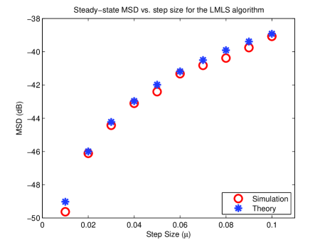
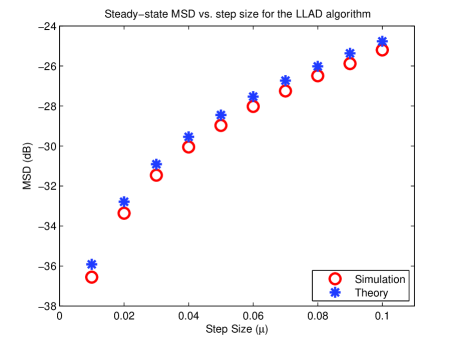
Refer to caption
(a) The LMLS Algorithm
Refer to caption
(b) The LLAD Algorithm
Figure 3: Dependence of the steady-state MSD on the step size μ𝜇\mu for the LMLS and LLAD algorithms.
Refer to caption
(a) MSD
Refer to caption
(b) EMSE
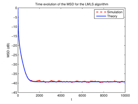
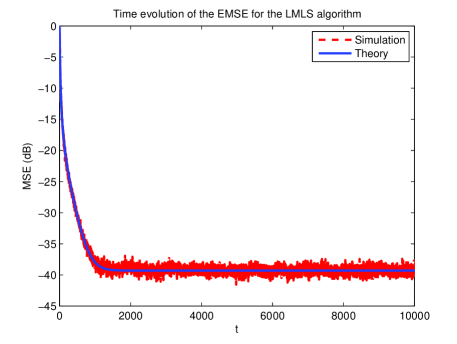
Figure 4: Theoretical and simulated MSD and EMSE for the LMLS algorithm.
Refer to caption
(a) MSD
Refer to caption
(b) EMSE
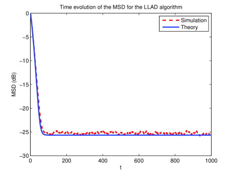
Figure 5: Theoretical and simulated MSD and EMSE for the LLAD algorithm.

IV-B Steady State Analysis

At the steady state, (13) and (17) yields

μE[𝐱t𝚺2]hU(et)=2hG(et)E[ea,t𝚺ea,t].𝜇𝐸delimited-[]superscriptsubscriptnormsubscript𝐱𝑡𝚺2subscript𝑈subscript𝑒𝑡2subscript𝐺subscript𝑒𝑡𝐸delimited-[]superscriptsubscript𝑒𝑎𝑡𝚺subscript𝑒𝑎𝑡\displaystyle\mu E\left[\|\mbox{$\mathbf{x}$}_{t}\|_{\mbox{$\mathbf{\Sigma}$}}^{2}\right]h_{U}(e_{t})=2\,h_{G}(e_{t})E\left[e_{a,t}^{\mbox{$\mathbf{\Sigma}$}}e_{a,t}\right]. (19)

Without loss of generality, we set the weight matrix 𝚺=𝐈𝚺𝐈\mbox{$\mathbf{\Sigma}$}=\mbox{$\mathbf{I}$}, then (19) leads the steady state EMSE

ζ𝜁\displaystyle\zeta =E[ea,t2]superscriptabsent𝐸delimited-[]superscriptsubscript𝑒𝑎𝑡2\displaystyle\stackrel{{\scriptstyle\bigtriangleup}}{{=}}E[e_{a,t}^{2}]
=μ2E[𝐱t2]hU(et)hG(et)absent𝜇2𝐸delimited-[]superscriptnormsubscript𝐱𝑡2subscript𝑈subscript𝑒𝑡subscript𝐺subscript𝑒𝑡\displaystyle=\frac{\mu}{2}E\left[\|\mbox{$\mathbf{x}$}_{t}\|^{2}\right]\frac{h_{U}(e_{t})}{h_{G}(e_{t})}
=μ2Tr(𝐑)hU(et)hG(et).absent𝜇2Tr𝐑subscript𝑈subscript𝑒𝑡subscript𝐺subscript𝑒𝑡\displaystyle=\frac{\mu}{2}\mathrm{Tr}(\mbox{$\mathbf{R}$})\frac{h_{U}(e_{t})}{h_{G}(e_{t})}. (20)

By Assumption 1, the steady state MSD is given by [23]

η𝜂\displaystyle\eta =E[𝐰~t2]superscriptabsent𝐸delimited-[]superscriptnormsubscript~𝐰𝑡2\displaystyle\stackrel{{\scriptstyle\bigtriangleup}}{{=}}E\left[\|\tilde{\mbox{$\mathbf{w}$}}_{t}\|^{2}\right]
=pTr(𝐑)ζ,absent𝑝Tr𝐑𝜁\displaystyle=\frac{p}{\mathrm{Tr}(\mbox{$\mathbf{R}$})}\zeta,

where p𝑝p denotes the filter length.

At the steady state, we additionally use the following assumptions, which directly follow from the property of a learning algorithm that as t𝑡t goes to infinity, etsubscript𝑒𝑡e_{t} goes to zero.

Assumption 5:

For sufficiently small μ𝜇\mu, hG(et)subscript𝐺subscript𝑒𝑡h_{G}(e_{t}) and hU(et)subscript𝑈subscript𝑒𝑡h_{U}(e_{t}) functions of the LMLS algorithm as t𝑡t\rightarrow\infty is given by

hG(et)=1σe2E[αet41+αet2]ασe2E[et4],subscript𝐺subscript𝑒𝑡1superscriptsubscript𝜎𝑒2𝐸delimited-[]𝛼superscriptsubscript𝑒𝑡41𝛼superscriptsubscript𝑒𝑡2𝛼superscriptsubscript𝜎𝑒2𝐸delimited-[]superscriptsubscript𝑒𝑡4\displaystyle h_{G}(e_{t})=\frac{1}{\sigma_{e}^{2}}E\left[\frac{\alpha e_{t}^{4}}{1+\alpha e_{t}^{2}}\right]\rightarrow\frac{\alpha}{\sigma_{e}^{2}}E\left[e_{t}^{4}\right],
hU(et)=E[α2et6(1+αet2)2]α2E[et6].subscript𝑈subscript𝑒𝑡𝐸delimited-[]superscript𝛼2superscriptsubscript𝑒𝑡6superscript1𝛼superscriptsubscript𝑒𝑡22superscript𝛼2𝐸delimited-[]superscriptsubscript𝑒𝑡6\displaystyle h_{U}(e_{t})=E\left[\frac{\alpha^{2}e_{t}^{6}}{\left(1+\alpha e_{t}^{2}\right)^{2}}\right]\rightarrow\alpha^{2}E\left[e_{t}^{6}\right].
Assumption 6:

For sufficiently small μ𝜇\mu, hG(et)subscript𝐺subscript𝑒𝑡h_{G}(e_{t}) and hU(et)subscript𝑈subscript𝑒𝑡h_{U}(e_{t}) functions of the LLAD algorithm as t𝑡t\rightarrow\infty is given by

hG(et)=1σe2E[αet21+α|et|]ασe2E[et2],subscript𝐺subscript𝑒𝑡1superscriptsubscript𝜎𝑒2𝐸delimited-[]𝛼superscriptsubscript𝑒𝑡21𝛼subscript𝑒𝑡𝛼superscriptsubscript𝜎𝑒2𝐸delimited-[]superscriptsubscript𝑒𝑡2\displaystyle h_{G}(e_{t})=\frac{1}{\sigma_{e}^{2}}E\left[\frac{\alpha e_{t}^{2}}{1+\alpha|e_{t}|}\right]\rightarrow\frac{\alpha}{\sigma_{e}^{2}}E\left[e_{t}^{2}\right],
hU(et)=E[α2et2(1+α|et|)2]α2E[et2].subscript𝑈subscript𝑒𝑡𝐸delimited-[]superscript𝛼2superscriptsubscript𝑒𝑡2superscript1𝛼subscript𝑒𝑡2superscript𝛼2𝐸delimited-[]superscriptsubscript𝑒𝑡2\displaystyle h_{U}(e_{t})=E\left[\frac{\alpha^{2}e_{t}^{2}}{\left(1+\alpha|e_{t}|\right)^{2}}\right]\rightarrow\alpha^{2}E\left[e_{t}^{2}\right].

Now, we explicitly derive the steady state analysis of the LMLS and LLAD algorithms, respectively.

The LMLS Algorithm: For the LMLS algorithm, by Assumption 5, (20) leads

ζLMLS=μ2αTr(𝐑)σe2E[et6]E[et4].subscript𝜁LMLS𝜇2𝛼Tr𝐑superscriptsubscript𝜎𝑒2𝐸delimited-[]subscriptsuperscript𝑒6𝑡𝐸delimited-[]subscriptsuperscript𝑒4𝑡\displaystyle\zeta_{\mathrm{LMLS}}=\frac{\mu}{2}\alpha\mathrm{Tr}(\mbox{$\mathbf{R}$})\sigma_{e}^{2}\frac{E\left[e^{6}_{t}\right]}{E\left[e^{4}_{t}\right]}. (21)

By Assumption 2, etsubscript𝑒𝑡e_{t} is a Gaussian random variable and σe2=ζ+σn2superscriptsubscript𝜎𝑒2𝜁superscriptsubscript𝜎𝑛2\sigma_{e}^{2}=\zeta+\sigma_{n}^{2}, we have

ζLMLSsubscript𝜁LMLS\displaystyle\zeta_{\mathrm{LMLS}} =μ2αTr(𝐑)σe215σe63σe4,absent𝜇2𝛼Tr𝐑superscriptsubscript𝜎𝑒215superscriptsubscript𝜎𝑒63superscriptsubscript𝜎𝑒4\displaystyle=\frac{\mu}{2}\alpha\mathrm{Tr}(\mbox{$\mathbf{R}$})\sigma_{e}^{2}\frac{15\sigma_{e}^{6}}{3\sigma_{e}^{4}},
=5μ2αTr(𝐑)(ζLMLS+σn2)2.absent5𝜇2𝛼Tr𝐑superscriptsubscript𝜁𝐿𝑀𝐿𝑆superscriptsubscript𝜎𝑛22\displaystyle=\frac{5\mu}{2}\alpha\mathrm{Tr}(\mbox{$\mathbf{R}$})\left(\zeta_{LMLS}+\sigma_{n}^{2}\right)^{2}.

Hence, after some algebra, the EMSE and MSD for the LMLS algorithm are given by

ζLMLS=15αμTr(𝐑)σn2±110αμTr(𝐑)σn25αμTr(𝐑),subscript𝜁LMLSplus-or-minus15𝛼𝜇Tr𝐑superscriptsubscript𝜎𝑛2110𝛼𝜇Tr𝐑superscriptsubscript𝜎𝑛25𝛼𝜇Tr𝐑\displaystyle\zeta_{\mathrm{LMLS}}=\frac{1-5\alpha\mu\mathrm{Tr}(\mbox{$\mathbf{R}$})\sigma_{n}^{2}\pm\sqrt{1-10\alpha\mu\mathrm{Tr}(\mbox{$\mathbf{R}$})\sigma_{n}^{2}}}{5\alpha\mu\mathrm{Tr}(\mbox{$\mathbf{R}$})}, (22)
ηLMLS=p15αμTr(𝐑)σn2±110αμTr(𝐑)σn25αμTr(𝐑)2,subscript𝜂LMLS𝑝plus-or-minus15𝛼𝜇Tr𝐑superscriptsubscript𝜎𝑛2110𝛼𝜇Tr𝐑superscriptsubscript𝜎𝑛25𝛼𝜇Trsuperscript𝐑2\displaystyle\eta_{\mathrm{LMLS}}=p\frac{1-5\alpha\mu\mathrm{Tr}(\mbox{$\mathbf{R}$})\sigma_{n}^{2}\pm\sqrt{1-10\alpha\mu\mathrm{Tr}(\mbox{$\mathbf{R}$})\sigma_{n}^{2}}}{5\alpha\mu\mathrm{Tr}(\mbox{$\mathbf{R}$})^{2}},

where the smaller roots match with the simulations. Note that (22) for α=1𝛼1\alpha=1 is the same with the EMSE of the LMF algorithm [23].

Remark 4.2: In (22), let μ~=μαsuperscript~𝜇𝜇𝛼\tilde{\mu}\stackrel{{\scriptstyle\bigtriangleup}}{{=}}\mu\alpha, then

ζLMLS=15μ~Tr(𝐑)σn2±110μ~Tr(𝐑)σn25μ~Tr(𝐑).subscript𝜁LMLSplus-or-minus15~𝜇Tr𝐑superscriptsubscript𝜎𝑛2110~𝜇Tr𝐑superscriptsubscript𝜎𝑛25~𝜇Tr𝐑\displaystyle\zeta_{\mathrm{LMLS}}=\frac{1-5\tilde{\mu}\mathrm{Tr}(\mbox{$\mathbf{R}$})\sigma_{n}^{2}\pm\sqrt{1-10\tilde{\mu}\mathrm{Tr}(\mbox{$\mathbf{R}$})\sigma_{n}^{2}}}{5\tilde{\mu}\mathrm{Tr}(\mbox{$\mathbf{R}$})}. (23)

By (23), we could achieve similar steady state convergence performance for different α𝛼\alpha by changing the step size μ𝜇\mu, e.g., μ~=μα=μ1010α~𝜇𝜇𝛼𝜇1010𝛼\tilde{\mu}=\mu\alpha=\frac{\mu}{10}10\alpha, however, smaller α𝛼\alpha results in a slower convergence rate. Hence, without loss of generality, we propose the algorithms with α=1𝛼1\alpha=1 under the Gaussianity assumption.

The LLAD Algorithm: Similarly, for the LLAD algorithm, by Assumption 6, (20) yields

ζLLADsubscript𝜁LLAD\displaystyle\zeta_{\mathrm{LLAD}} =μ2Tr(𝐑)σe2αE[et2]E[et2],absent𝜇2Tr𝐑superscriptsubscript𝜎𝑒2𝛼𝐸delimited-[]subscriptsuperscript𝑒2𝑡𝐸delimited-[]subscriptsuperscript𝑒2𝑡\displaystyle=\frac{\mu}{2}\mathrm{Tr}(\mbox{$\mathbf{R}$})\sigma_{e}^{2}\alpha\frac{E[e^{2}_{t}]}{E[e^{2}_{t}]},
=μα2Tr(𝐑)σe2.absent𝜇𝛼2Tr𝐑superscriptsubscript𝜎𝑒2\displaystyle=\frac{\mu\alpha}{2}\mathrm{Tr}(\mbox{$\mathbf{R}$})\sigma_{e}^{2}.

By Assumption 2, the EMSE and MSD for the LLAD algorithm is given by

ζLLAD=μαTr(𝐑)σn22μαTr(𝐑).subscript𝜁LLAD𝜇𝛼Tr𝐑superscriptsubscript𝜎𝑛22𝜇𝛼Tr𝐑\displaystyle\zeta_{\mathrm{LLAD}}=\frac{\mu\alpha\mathrm{Tr}(\mbox{$\mathbf{R}$})\sigma_{n}^{2}}{2-\mu\alpha\mathrm{Tr}(\mbox{$\mathbf{R}$})}. (24)
ηLLAD=μαpσn22μαTr(𝐑)subscript𝜂LLAD𝜇𝛼𝑝superscriptsubscript𝜎𝑛22𝜇𝛼Tr𝐑\displaystyle\eta_{\mathrm{LLAD}}=\frac{\mu\alpha p\sigma_{n}^{2}}{2-\mu\alpha\mathrm{Tr}(\mbox{$\mathbf{R}$})}

Note that (24) is the same with the EMSE of the LMS algorithm [23]. Hence, for sufficiently small α𝛼\alpha, the LLAD algorithm achieves similar steady-state convergence performance with the LMS algorithm under the zero-mean Gaussian error signal assumption.

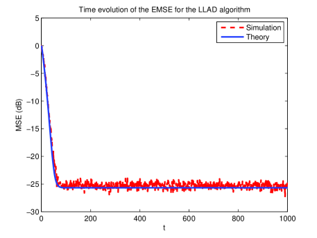
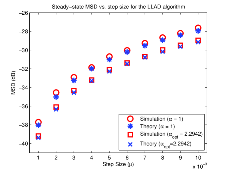
In Fig. 3, we plot the theoretical and simulated MSD vs. step size for the LMLS and LLAD algorithms. In the system identification framework, we choose the regressor and noise signals as i.i.d. zero mean Gaussian with the variances σx2=1superscriptsubscript𝜎𝑥21\sigma_{x}^{2}=1 and σn2=0.01superscriptsubscript𝜎𝑛20.01\sigma_{n}^{2}=0.01, respectively. The parameter of interest 𝐰o5subscript𝐰𝑜superscript5\mbox{$\mathbf{w}$}_{o}\in\mathbbm{R}^{5} is randomly chosen. We observe that the theoretical steady-state MSD matches with the simulation results generated through the ensemble average of the last 103superscript10310^{3} iterations of 105superscript10510^{5} (for the LMLS algorithm) and 104superscript10410^{4} (for the LLAD algorithm) iterations of 200 independent trials. In. Fig. 4 and Fig. 5, under the same configurations, we compare the simulated MSD and EMSE curves generated through the ensemble average of 200 independent trials with the theoretical results for the step-size μ=0.1𝜇0.1\mu=0.1. We note that theoretical performance analyzes match with our simulation results.

IV-C Tracking Performance

In this subsection, we investigate the tracking performance of the introduced algorithms in a non-stationary environment. We assume a random walk model [1] for 𝐰o,tsubscript𝐰𝑜𝑡\mbox{$\mathbf{w}$}_{o,t} such that

𝐰o,t+1=𝐰o,t+𝐪tsubscript𝐰𝑜𝑡1subscript𝐰𝑜𝑡subscript𝐪𝑡\displaystyle\mbox{$\mathbf{w}$}_{o,t+1}=\mbox{$\mathbf{w}$}_{o,t}+\mbox{$\mathbf{q}$}_{t} (25)

where 𝐪tpsubscript𝐪𝑡superscript𝑝\mbox{$\mathbf{q}$}_{t}\in\mbox{$\mathbbm{R}^{p}$} is a zero-mean vector process with covariance matrix E[𝐪t𝐪tT]=𝐐𝐸delimited-[]subscript𝐪𝑡superscriptsubscript𝐪𝑡𝑇𝐐E[\mbox{$\mathbf{q}$}_{t}\mbox{$\mathbf{q}$}_{t}^{T}]=\mbox{$\mathbf{Q}$}. We note that the model (25) has not changed the definitions of a priori error. Hence, by the Assumption 5, the tracking EMSE of the LMLS is the same with the tracking EMSE of the LMF and is approximately given by [1]

ζLMLS3αμσn4Tr(𝐑)+μ1Tr(𝐐)6σn2.superscriptsubscript𝜁LMLS3𝛼𝜇superscriptsubscript𝜎𝑛4Tr𝐑superscript𝜇1Tr𝐐6superscriptsubscript𝜎𝑛2\displaystyle\zeta_{\mathrm{LMLS}}^{\prime}\approx\frac{3\alpha\mu\sigma_{n}^{4}\mathrm{Tr}(\mbox{$\mathbf{R}$})+\mu^{-1}\mathrm{Tr}(\mbox{$\mathbf{Q}$})}{6\sigma_{n}^{2}}.

Similarly, through the Assumption 6, we obtain the tracking EMSE of the LLAD as

ζLLAD=αμσn2Tr(𝐑)+μ1Tr(𝐐)2αμTr(𝐑).superscriptsubscript𝜁LLAD𝛼𝜇superscriptsubscript𝜎𝑛2Tr𝐑superscript𝜇1Tr𝐐2𝛼𝜇Tr𝐑\displaystyle\zeta_{\mathrm{LLAD}}^{\prime}=\frac{\alpha\mu\sigma_{n}^{2}\mathrm{Tr}(\mbox{$\mathbf{R}$})+\mu^{-1}\mathrm{Tr}(\mbox{$\mathbf{Q}$})}{2-\alpha\mu\mathrm{Tr}(\mbox{$\mathbf{R}$})}.

In the next section, we compare the new algorithms with the conventional LMS and SA in terms of the stability bound and robustness.

V Comparison with the Conventional Algorithms

We re-emphasize that the cost function J(et)𝐽subscript𝑒𝑡J(e_{t}) intrinsically combines the costs, mainly, F(et)𝐹subscript𝑒𝑡F(e_{t}) and F2(et)superscript𝐹2subscript𝑒𝑡F^{2}(e_{t}) based on the relative error amount since for small perturbations on the error, the updates are mainly using the cost F2(et)superscript𝐹2subscript𝑒𝑡F^{2}(e_{t}). Based on our stochastic gradient approach, i.e., removing the expectation in the gradient descent, F2(et)superscript𝐹2subscript𝑒𝑡F^{2}(e_{t}) and F(et2)𝐹superscriptsubscript𝑒𝑡2F(e_{t}^{2}) results in the same algorithm. Hence, in this section we compare the stability of the LMLS algorithm with the LMF and LMS algorithms and analyze the robustness of the LLAD algorithm in the impulsive noise environments.

V-A Stability Bound for the LMLS Algorithm

We again refer to the stochastic gradient update (9), which we rewrite as

𝐰t+1=𝐰t+μ𝐱tetf(et),subscript𝐰𝑡1subscript𝐰𝑡superscript𝜇subscript𝐱𝑡subscriptsubscript𝑒𝑡𝑓subscript𝑒𝑡\displaystyle\mbox{$\mathbf{w}$}_{t+1}=\mbox{$\mathbf{w}$}_{t}+\mu^{\prime}\mbox{$\mathbf{x}$}_{t}\nabla_{e_{t}}f(e_{t}),

where μ=μαf(et)1+αf(et)superscriptsuperscript𝜇𝜇𝛼𝑓subscript𝑒𝑡1𝛼𝑓subscript𝑒𝑡\mu^{\prime}\stackrel{{\scriptstyle\bigtriangleup}}{{=}}\mu\frac{\alpha f(e_{t})}{1+\alpha f(e_{t})}. Note that μμsuperscript𝜇𝜇\mu^{\prime}\leq\mu irrespective of the design parameter α𝛼\alpha. Hence, intuitively we can state that for the introduced algorithms the step-size bound is at least as large as the step-size bound for the corresponding conventional algorithm.

Analytically, for stable updates the step size μ𝜇\mu should satisfy

E[𝐰~t+12]E[𝐰~t2].𝐸delimited-[]superscriptnormsubscript~𝐰𝑡12𝐸delimited-[]superscriptnormsubscript~𝐰𝑡2\displaystyle E\left[\|\tilde{\mbox{$\mathbf{w}$}}_{t+1}\|^{2}\right]\leq E\left[\|\tilde{\mbox{$\mathbf{w}$}}_{t}\|^{2}\right].

By (13), the Assumption 3, and 𝚺=𝐈𝚺𝐈\mbox{$\mathbf{\Sigma}$}=\mbox{$\mathbf{I}$}, the stability bound on the step size is given by

μ2E[𝐱t2]infE[ea,t2]Ω{E[ea,tet]hG(et)hU(et)},𝜇2𝐸delimited-[]superscriptnormsubscript𝐱𝑡2𝐸delimited-[]superscriptsubscript𝑒𝑎𝑡2Ωinf𝐸delimited-[]subscript𝑒𝑎𝑡subscript𝑒𝑡subscript𝐺subscript𝑒𝑡subscript𝑈subscript𝑒𝑡\displaystyle\mu\leq\frac{2}{E\left[\|\mbox{$\mathbf{x}$}_{t}\|^{2}\right]}\underset{E[e_{a,t}^{2}]\in\Omega}{\mathrm{inf}}\left\{E[e_{a,t}e_{t}]\frac{h_{G}(e_{t})}{h_{U}(e_{t})}\right\},

where

Ω={E[ea,t2]:λE[ea,t2]14Tr(𝐑)E[𝐰~02]},superscriptΩconditional-set𝐸delimited-[]superscriptsubscript𝑒𝑎𝑡2𝜆𝐸delimited-[]superscriptsubscript𝑒𝑎𝑡214Tr𝐑𝐸delimited-[]superscriptnormsubscript~𝐰02\displaystyle\Omega\stackrel{{\scriptstyle\bigtriangleup}}{{=}}\left\{E[e_{a,t}^{2}]:\lambda\leq E[e_{a,t}^{2}]\leq\frac{1}{4}\mathrm{Tr}(\mbox{$\mathbf{R}$})E[\|\tilde{\mbox{$\mathbf{w}$}}_{0}\|^{2}]\right\},

with the Cramer-Rao lower bound λ𝜆\lambda [27]. For example the step size bound for the LMLS yields

μ1E[𝐱t2]infE[ea,t2]Ω{E[ea,tet]E[et2]β},𝜇1𝐸delimited-[]superscriptnormsubscript𝐱𝑡2𝐸delimited-[]superscriptsubscript𝑒𝑎𝑡2Ωinf𝐸delimited-[]subscript𝑒𝑎𝑡subscript𝑒𝑡𝐸delimited-[]subscriptsuperscript𝑒2𝑡𝛽\displaystyle\mu\leq\frac{1}{E\left[\|\mbox{$\mathbf{x}$}_{t}\|^{2}\right]}\underset{E[e_{a,t}^{2}]\in\Omega}{\mathrm{inf}}\left\{\frac{E[e_{a,t}e_{t}]}{E\left[e^{2}_{t}\right]}\beta\right\},

where

β=superscript𝛽absent\displaystyle\beta\stackrel{{\scriptstyle\bigtriangleup}}{{=}} E[αet41+αet2]E[α2et6(1+αet2)2]𝐸delimited-[]𝛼subscriptsuperscript𝑒4𝑡1𝛼subscriptsuperscript𝑒2𝑡𝐸delimited-[]superscript𝛼2subscriptsuperscript𝑒6𝑡superscript1𝛼subscriptsuperscript𝑒2𝑡2\displaystyle\frac{E\left[\frac{\alpha e^{4}_{t}}{1+\alpha e^{2}_{t}}\right]}{E\left[\frac{\alpha^{2}e^{6}_{t}}{\left(1+\alpha e^{2}_{t}\right)^{2}}\right]}
=\displaystyle= E[αet4(1+αet2)2]+E[α2et6(1+αet2)2]E[α2et6(1+αet2)2]1.𝐸delimited-[]𝛼subscriptsuperscript𝑒4𝑡superscript1𝛼subscriptsuperscript𝑒2𝑡2𝐸delimited-[]superscript𝛼2subscriptsuperscript𝑒6𝑡superscript1𝛼subscriptsuperscript𝑒2𝑡2𝐸delimited-[]superscript𝛼2subscriptsuperscript𝑒6𝑡superscript1𝛼subscriptsuperscript𝑒2𝑡21\displaystyle\frac{E\left[\frac{\alpha e^{4}_{t}}{\left(1+\alpha e^{2}_{t}\right)^{2}}\right]+E\left[\frac{\alpha^{2}e^{6}_{t}}{\left(1+\alpha e^{2}_{t}\right)^{2}}\right]}{E\left[\frac{\alpha^{2}e^{6}_{t}}{\left(1+\alpha e^{2}_{t}\right)^{2}}\right]}\geq 1.

We re-emphasize that the LMLS extends the stability bound of the LMS algorithm (the same bound with β=1𝛽1\beta=1) while performing comparable performance with the LMF algorithm, which has several stability issues [3, 4, 5].

V-B Robustness Analysis for the LLAD Algorithm

Although the performance analysis of the adaptive filters assumes the white Gaussian noise signals, in practical applications the impulsive noise is a common problem [8]. In order to analyze the performance in the impulsive noise environments, we use the following model.

Impulsive noise model: We model the noise as a summation of two independent random terms [28, 29] as

nt=no,t+btni,t,subscript𝑛𝑡subscript𝑛𝑜𝑡subscript𝑏𝑡subscript𝑛𝑖𝑡\displaystyle n_{t}=n_{o,t}+b_{t}n_{i,t},

where no,tsubscript𝑛𝑜𝑡n_{o,t} is the ordinary noise signal that is zero-mean Gaussian with variance σno2superscriptsubscript𝜎subscript𝑛𝑜2\sigma_{n_{o}}^{2} and ni,tsubscript𝑛𝑖𝑡n_{i,t} is the impulse-noise that is also zero-mean Gaussian with significantly large variance σni2superscriptsubscript𝜎subscript𝑛𝑖2\sigma_{n_{i}}^{2}. Here, btsubscript𝑏𝑡b_{t} is generated through a Bernoulli random process and determines the occurrence of the impulses in the noise signal with pB(bt=1)=νisubscript𝑝𝐵subscript𝑏𝑡1subscript𝜈𝑖p_{B}(b_{t}=1)=\nu_{i} and pB(bt=0)=1νisubscript𝑝𝐵subscript𝑏𝑡01subscript𝜈𝑖p_{B}(b_{t}=0)=1-\nu_{i} where νisubscript𝜈𝑖\nu_{i} is the frequency of the impulses in the noise signal. The corresponding probability density function is given by

pn(nt)=1νi2πσnoexp(nt22σno2)+νi2πσnexp(nt22σn2),subscript𝑝𝑛subscript𝑛𝑡1subscript𝜈𝑖2𝜋subscript𝜎subscript𝑛𝑜expsubscriptsuperscript𝑛2𝑡2superscriptsubscript𝜎subscript𝑛𝑜2subscript𝜈𝑖2𝜋subscript𝜎𝑛expsubscriptsuperscript𝑛2𝑡2superscriptsubscript𝜎𝑛2\displaystyle p_{n}(n_{t})=\frac{1-\nu_{i}}{\sqrt{2\pi}\sigma_{n_{o}}}\mathrm{exp}\left(-\frac{n^{2}_{t}}{2\sigma_{n_{o}}^{2}}\right)+\frac{\nu_{i}}{\sqrt{2\pi}\sigma_{n}}\mathrm{exp}\left(-\frac{n^{2}_{t}}{2\sigma_{n}^{2}}\right),

where σn2=σno2+σni2superscriptsubscript𝜎𝑛2superscriptsubscript𝜎subscript𝑛𝑜2superscriptsubscript𝜎subscript𝑛𝑖2\sigma_{n}^{2}=\sigma_{n_{o}}^{2}+\sigma_{n_{i}}^{2}.

We particularly analyze the steady-state performance of the LLAD algorithm (for which f(et)=|et|𝑓subscript𝑒𝑡subscript𝑒𝑡f(e_{t})=|e_{t}|) in the impulsive noise environments since we motivate the LLAD algorithm as improving the steady state convergence performance of the SA. Since the noise is not a Gaussian random variable in impulsive noise environment, the Gaussianity assumption of the estimation error etsubscript𝑒𝑡e_{t} and the Price’s Theorem are not applicable. At the steady-state, for 𝚺=𝐈𝚺𝐈\mbox{$\mathbf{\Sigma}$}=\mbox{$\mathbf{I}$}, (13) yields

E[𝐱t2]=2E[αea,tet1+α|et|]μE[α2et2(1+α|et|)2].𝐸delimited-[]superscriptnormsubscript𝐱𝑡22𝐸delimited-[]𝛼subscript𝑒𝑎𝑡subscript𝑒𝑡1𝛼subscript𝑒𝑡𝜇𝐸delimited-[]superscript𝛼2subscriptsuperscript𝑒2𝑡superscript1𝛼subscript𝑒𝑡2\displaystyle E\left[\|\mbox{$\mathbf{x}$}_{t}\|^{2}\right]=\frac{2E\left[\frac{\alpha e_{a,t}e_{t}}{1+\alpha|e_{t}|}\right]}{\mu E\left[\frac{\alpha^{2}e^{2}_{t}}{\left(1+\alpha|e_{t}|\right)^{2}}\right]}. (26)

We now evaluate the each term in (26) separately. We first consider the nominator of the RHS of (26), and write

E[αea,tet1+α|et|]𝐸delimited-[]𝛼subscript𝑒𝑎𝑡subscript𝑒𝑡1𝛼subscript𝑒𝑡\displaystyle E\left[\frac{\alpha e_{a,t}e_{t}}{1+\alpha|e_{t}|}\right]
=αea,t(ea,t+nt)1+α|ea,t+nt|exp(ea,t22σea2)2πσeapn(nt)𝑑ea,t𝑑nt.absentsuperscriptsubscriptsuperscriptsubscript𝛼subscript𝑒𝑎𝑡subscript𝑒𝑎𝑡subscript𝑛𝑡1𝛼subscript𝑒𝑎𝑡subscript𝑛𝑡expsuperscriptsubscript𝑒𝑎𝑡22superscriptsubscript𝜎subscript𝑒𝑎22𝜋subscript𝜎subscript𝑒𝑎subscript𝑝𝑛subscript𝑛𝑡differential-dsubscript𝑒𝑎𝑡differential-dsubscript𝑛𝑡\displaystyle=\int_{-\infty}^{\infty}\int_{-\infty}^{\infty}\frac{\alpha e_{a,t}(e_{a,t}+n_{t})}{1+\alpha|e_{a,t}+n_{t}|}\frac{\mathrm{exp}\left(-\frac{e_{a,t}^{2}}{2\sigma_{e_{a}}^{2}}\right)}{\sqrt{2\pi}\sigma_{e_{a}}}p_{n}(n_{t})de_{a,t}dn_{t}.
=αea,tetexp(ea,t22σea2nt22σno2)2πσeaσno(1νi)𝑑ea,t𝑑ntabsent𝛼superscriptsubscriptsuperscriptsubscriptsubscript𝑒𝑎𝑡subscript𝑒𝑡expsuperscriptsubscript𝑒𝑎𝑡22superscriptsubscript𝜎subscript𝑒𝑎2subscriptsuperscript𝑛2𝑡2superscriptsubscript𝜎subscript𝑛𝑜22𝜋subscript𝜎subscript𝑒𝑎subscript𝜎subscript𝑛𝑜1subscript𝜈𝑖differential-dsubscript𝑒𝑎𝑡differential-dsubscript𝑛𝑡\displaystyle=\alpha\int_{-\infty}^{\infty}\int_{-\infty}^{\infty}e_{a,t}e_{t}\frac{\mathrm{exp}\left(-\frac{e_{a,t}^{2}}{2\sigma_{e_{a}}^{2}}-\frac{n^{2}_{t}}{2\sigma_{n_{o}}^{2}}\right)}{2\pi\sigma_{e_{a}}\sigma_{n_{o}}}(1-\nu_{i})de_{a,t}dn_{t}
+ea,tsign(ea,t+nt)exp(ea,t22σea2nt22σn2)2πσeaσnνi𝑑ea,t𝑑nt,superscriptsubscriptsuperscriptsubscriptsubscript𝑒𝑎𝑡signsubscript𝑒𝑎𝑡subscript𝑛𝑡expsuperscriptsubscript𝑒𝑎𝑡22superscriptsubscript𝜎subscript𝑒𝑎2subscriptsuperscript𝑛2𝑡2superscriptsubscript𝜎𝑛22𝜋subscript𝜎subscript𝑒𝑎subscript𝜎𝑛subscript𝜈𝑖differential-dsubscript𝑒𝑎𝑡differential-dsubscript𝑛𝑡\displaystyle\hskip 2.84544pt+\int_{-\infty}^{\infty}\int_{-\infty}^{\infty}e_{a,t}\mathrm{sign}(e_{a,t}+n_{t})\frac{\mathrm{exp}\left(-\frac{e_{a,t}^{2}}{2\sigma_{e_{a}}^{2}}-\frac{n^{2}_{t}}{2\sigma_{n}^{2}}\right)}{2\pi\sigma_{e_{a}}\sigma_{n}}\nu_{i}de_{a,t}dn_{t},

where in the last step of the equation we assume that in the impulse-free environment, αea,tet1+α|et|αea,tet𝛼subscript𝑒𝑎𝑡subscript𝑒𝑡1𝛼subscript𝑒𝑡𝛼subscript𝑒𝑎𝑡subscript𝑒𝑡\frac{\alpha e_{a,t}e_{t}}{1+\alpha|e_{t}|}\approx\alpha e_{a,t}e_{t} since at steady state, the error is assumed to take relatively small values whereas if the impulse-noise occurs, αea,tet1+α|et|ea,tsign(et)𝛼subscript𝑒𝑎𝑡subscript𝑒𝑡1𝛼subscript𝑒𝑡subscript𝑒𝑎𝑡signsubscript𝑒𝑡\frac{\alpha e_{a,t}e_{t}}{1+\alpha|e_{t}|}\approx e_{a,t}\mathrm{sign}(e_{t}) due to the large perturbation on the error. Hence, since σn2σea2much-greater-thansuperscriptsubscript𝜎𝑛2superscriptsubscript𝜎subscript𝑒𝑎2\sigma_{n}^{2}\gg\sigma_{e_{a}}^{2}, the expectation leads

E[αea,tet1+α|et|]=α(1νi)σea2+2πνiσea2σn.𝐸delimited-[]𝛼subscript𝑒𝑎𝑡subscript𝑒𝑡1𝛼subscript𝑒𝑡𝛼1subscript𝜈𝑖superscriptsubscript𝜎subscript𝑒𝑎22𝜋subscript𝜈𝑖superscriptsubscript𝜎subscript𝑒𝑎2subscript𝜎𝑛\displaystyle E\left[\frac{\alpha e_{a,t}e_{t}}{1+\alpha|e_{t}|}\right]=\alpha(1-\nu_{i})\sigma_{e_{a}}^{2}+\sqrt{\frac{2}{\pi}}\nu_{i}\frac{\sigma_{e_{a}}^{2}}{\sigma_{n}}. (27)

Following similar steps for the denominator of the RHS of (26), we obtain

E[α2et2(1+α|et|)2]=α2(1νi)(σea2+σno2)+νi.𝐸delimited-[]superscript𝛼2subscriptsuperscript𝑒2𝑡superscript1𝛼subscript𝑒𝑡2superscript𝛼21subscript𝜈𝑖superscriptsubscript𝜎subscript𝑒𝑎2superscriptsubscript𝜎subscript𝑛𝑜2subscript𝜈𝑖\displaystyle E\left[\frac{\alpha^{2}e^{2}_{t}}{\left(1+\alpha|e_{t}|\right)^{2}}\right]=\alpha^{2}(1-\nu_{i})\left(\sigma_{e_{a}}^{2}+\sigma_{n_{o}}^{2}\right)+\nu_{i}. (28)

By (26), (27) and (28), the EMSE of the LLAD algorithm in the impulsive noise environment is given by

ζLLAD=μTr(𝐑)(νi+α2(1νi)σno2)α(1νi)(2αμTr(𝐑))+8πνiσn.superscriptsubscript𝜁LLAD𝜇Tr𝐑subscript𝜈𝑖superscript𝛼21subscript𝜈𝑖superscriptsubscript𝜎subscript𝑛𝑜2𝛼1subscript𝜈𝑖2𝛼𝜇Tr𝐑8𝜋subscript𝜈𝑖subscript𝜎𝑛\displaystyle\zeta_{\mathrm{LLAD}}^{*}=\frac{\mu\mathrm{Tr}(\mbox{$\mathbf{R}$})\left(\nu_{i}+\alpha^{2}(1-\nu_{i})\sigma_{n_{o}}^{2}\right)}{\alpha(1-\nu_{i})(2-\alpha\mu\mathrm{Tr}(\mbox{$\mathbf{R}$}))+\sqrt{\frac{8}{\pi}}\frac{\nu_{i}}{\sigma_{n}}}. (29)

Note that for νi=0subscript𝜈𝑖0\nu_{i}=0 (impulse-free) (29) yields (24).

Refer to caption
Figure 6: Dependence of the steady-state MSD on the step size μ𝜇\mu for the LLAD algorithm in the 5% impulsive noise environment.

Remark 5.1: Increasing νisubscript𝜈𝑖\nu_{i} or in other words more frequent impulses cause larger steady state EMSE. However, through the optimization of α𝛼\alpha, we can minimize the steady state EMSE. After some algebra, the optimum design parameter in impulsive noise environment is roughly given by

αoptνi1νi1σno.subscript𝛼optsubscript𝜈𝑖1subscript𝜈𝑖1subscript𝜎subscript𝑛𝑜\displaystyle\alpha_{\mathrm{opt}}\approx\sqrt{\frac{\nu_{i}}{1-\nu_{i}}}\frac{1}{\sigma_{n_{o}}}.

In Fig. 6, we plot the dependence of the steady-state MSD with the step size in 5%, i.e., νi=0.05subscript𝜈𝑖0.05\nu_{i}=0.05, impulsive noise environment where σx2=1superscriptsubscript𝜎𝑥21\sigma_{x}^{2}=1, σno2=0.01superscriptsubscript𝜎subscript𝑛𝑜20.01\sigma_{n_{o}}^{2}=0.01 and σni2=104superscriptsubscript𝜎subscript𝑛𝑖2superscript104\sigma_{n_{i}}^{2}=10^{4} after 200 independent trials. We observe that αoptsubscript𝛼opt\alpha_{\mathrm{opt}} improves the convergence performance and the theoretical analyzes through the impulsive noise model matches with the simulation results. We next demonstrate the performance of the introduced algorithms in different applications.

VI Numerical Examples

In this section, we particularly compare the convergence rate of the algorithms for the same steady state MSD through the specific choice of the step sizes for a fair comparison. Here, we have a stationary data dt=𝐰oT𝐱t+ntsubscript𝑑𝑡superscriptsubscript𝐰𝑜𝑇subscript𝐱𝑡subscript𝑛𝑡d_{t}=\mbox{$\mathbf{w}$}_{o}^{T}\mbox{$\mathbf{x}$}_{t}+n_{t} where 𝐱tsubscript𝐱𝑡\mbox{$\mathbf{x}$}_{t} is zero-mean Gaussian i.i.d. regression signal with variance σx2=1superscriptsubscript𝜎𝑥21\sigma_{x}^{2}=1, ntsubscript𝑛𝑡n_{t} represent zero-mean i.i.d. noise signal and the parameter of interest 𝐰o5subscript𝐰𝑜superscript5\mbox{$\mathbf{w}$}_{o}\in\mbox{$\mathbbm{R}$}^{5} is randomly chosen. In following scenarios, we compare the algorithms under Gaussian noise and impulsive noise models subsequently.

Scenario 1 (impulse-free environment):
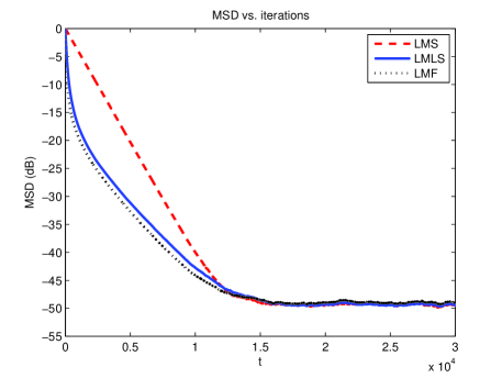
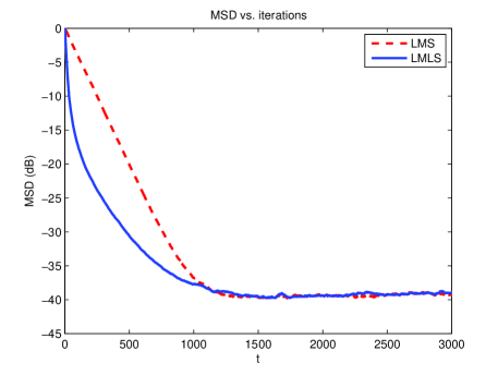
In that scenario, we use a zero-mean Gaussian i.i.d. noise signal with the variance σn2=0.01superscriptsubscript𝜎𝑛20.01\sigma_{n}^{2}=0.01 and the design parameter α=1𝛼1\alpha=1. In Fig. 7, we compare the convergence rate of the LMLS, LMF and LMS algorithms for relatively small step sizes. We observe that LMLS and LMF algorithms achieve comparable performance and LMLS achieves better convergence performance than the LMS algorithm. In Fig. 8, we compare the LMLS and LMS algorithms for relatively large step sizes, i.e., μLMLS=0.1subscript𝜇LMLS0.1\mu_{\mathrm{LMLS}}=0.1 and μLMS=0.0047subscript𝜇LMS0.0047\mu_{\mathrm{LMS}}=0.0047. We only compare the LMLS and LMS algorithms since the LMF algorithm is not stable for such a step-size. Hence, the LMLS algorithm demonstrate comparable convergence performance with the LMF algorithm with extended stability bound.

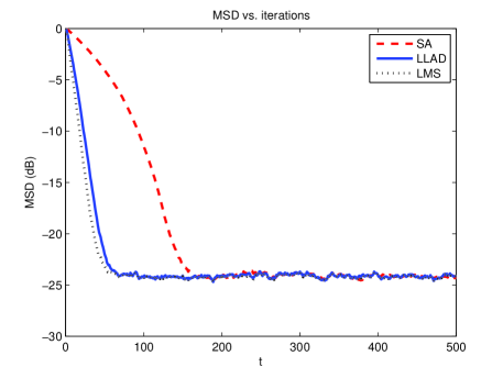
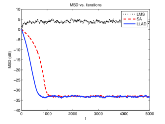
In Fig. 9, we compare the LLAD, SA and LMS algorithms in impulse-free noise environment. We observe that the LLAD algorithm shows comparable convergence performance with the LMS algorithm, in other words, the logarithmic error cost framework improves the convergence performance of the SA.
Refer to caption
Figure 7: Comparison of the MSD of the LMLS, LMS and LMF algorithms for the same steady state MSD where μLMLS=μLMF=0.01subscript𝜇LMLSsubscript𝜇LMF0.01\mu_{\mathrm{LMLS}}=\mu_{\mathrm{LMF}}=0.01 and μLMS=0.00047subscript𝜇LMS0.00047\mu_{\mathrm{LMS}}=0.00047.
Refer to caption
Figure 8: Comparison of the MSD of the LMLS and LMS algorithms for the same steady state MSD where μLMLS=0.1subscript𝜇LMLS0.1\mu_{\mathrm{LMLS}}=0.1 and μLMS=0.0047subscript𝜇LMS0.0047\mu_{\mathrm{LMS}}=0.0047.
Refer to caption
Figure 9: Comparison of the MSD of the LLAD, SA and LMS algorithms in impulse-free noise environment with μLLAD=0.12subscript𝜇LLAD0.12\mu_{\mathrm{LLAD}}=0.12, μSA=0.01subscript𝜇SA0.01\mu_{\mathrm{SA}}=0.01 and μLMS=0.1subscript𝜇LMS0.1\mu_{\mathrm{LMS}}=0.1.

Scenario 2 (impulsive noise environment):
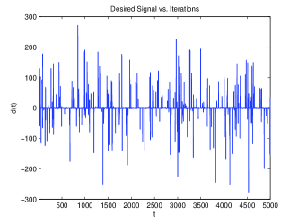
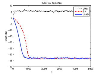
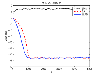
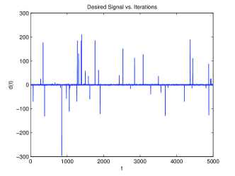
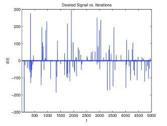
Here, we use the impulsive noise model with σni2=104superscriptsubscript𝜎subscript𝑛𝑖2superscript104\sigma_{n_{i}}^{2}=10^{4}. In that configuration, we resort to the design parameter since through the optimization of α𝛼\alpha, the LLAD algorithm could achieve smaller steady-state MSD. In Fig. 10, we plot sample desired signals in 1%, 2% and 5% impulsive noise environments and Fig. 11 shows the corresponding time evolution of the MSD of the LLAD, SA and LMS algorithms. The step sizes are chosen as μLLAD=μLMS=0.0097,0.007,0.0043formulae-sequencesubscript𝜇LLADsubscript𝜇LMS0.00970.0070.0043\mu_{\mathrm{LLAD}}=\mu_{\mathrm{LMS}}=0.0097,0.007,0.0043 for 1%, 2% and 5% impulsive noise environments, respectively, and μSA=0.0015subscript𝜇SA0.0015\mu_{\mathrm{SA}}=0.0015. The figures show that in the impulsive noise environments, the LMS algorithm does not converge while the LLAD algorithm, which achieves comparable convergence performance with the LMS algorithm in the impulse free environment, performs still better than the SA.
Refer to caption
(a) 1%
Refer to caption
(b) 2%
Refer to caption
(c) 5%
Figure 10: Desired signal in 1%, 2% and 5% impulsive noise environments.
Refer to caption
(a) 1% (αopt=1.005subscript𝛼𝑜𝑝𝑡1.005\alpha_{opt}=1.005)
Refer to caption
(b) 2% (αopt=1.4286subscript𝛼𝑜𝑝𝑡1.4286\alpha_{opt}=1.4286)
Refer to caption
(c) 5% (αopt=2.2942subscript𝛼𝑜𝑝𝑡2.2942\alpha_{opt}=2.2942)
Figure 11: Comparison of the MSD of the LLAD, SA and LMS algorithms in 1%, 2% and 5% impulsive noise environments.

VII Concluding Remarks

In this paper, we present a novel family of adaptive filtering algorithms based on the logarithmic error cost framework. We propose important members of the new family, i.e., the LMLS and LLAD algorithms. The LMLS algorithm achieves comparable convergence performance with the LMF algorithm with far larger stability bound on the step size. In the impulse-free environment, the LLAD algorithm has a similar convergence performance with the LMS algorithm. Furthermore, the LLAD algorithm is robust against impulsive interferences and outperforms the SA. We also provide comprehensive performance analyzes of the introduced algorithms, which match with our simulation results. For example, the steady-state analyzes in the impulse-free and impulsive noise environments. Finally, we show the improved convergence performance of the new algorithms in several different system identification scenarios.

Appendix A Evaluation of hG(et)subscript𝐺subscript𝑒𝑡h_{G}(e_{t})

The LMLS algorithm: We have

hG(et)subscript𝐺subscript𝑒𝑡\displaystyle h_{G}(e_{t}) =1σe2E[αet41+αet2],absent1superscriptsubscript𝜎𝑒2𝐸delimited-[]𝛼superscriptsubscript𝑒𝑡41𝛼superscriptsubscript𝑒𝑡2\displaystyle=\frac{1}{\sigma_{e}^{2}}E\left[\frac{\alpha e_{t}^{4}}{1+\alpha e_{t}^{2}}\right],
=1σe2(σe2α1+α1E[11+αet2]),absent1superscriptsubscript𝜎𝑒2superscriptsubscript𝜎𝑒2superscript𝛼1superscript𝛼1𝐸delimited-[]11𝛼superscriptsubscript𝑒𝑡2\displaystyle=\frac{1}{\sigma_{e}^{2}}\left(\sigma_{e}^{2}-\alpha^{-1}+\alpha^{-1}E\left[\frac{1}{1+\alpha e_{t}^{2}}\right]\right), (30)

where σe2=E[et2]superscriptsubscript𝜎𝑒2𝐸delimited-[]subscriptsuperscript𝑒2𝑡\sigma_{e}^{2}=E[e^{2}_{t}] and the first line of the equation follows according to the definition of g(et)𝑔subscript𝑒𝑡g(e_{t}) in (14). According to Assumption 2, we obtain the last term in (A) as follows

E[11+αet2]𝐸delimited-[]11𝛼subscriptsuperscript𝑒2𝑡\displaystyle E\left[\frac{1}{1+\alpha e^{2}_{t}}\right] =12πσe11+αet2exp(et22σe2)𝑑etabsent12𝜋subscript𝜎𝑒superscriptsubscript11𝛼subscriptsuperscript𝑒2𝑡expsubscriptsuperscript𝑒2𝑡2superscriptsubscript𝜎𝑒2differential-dsubscript𝑒𝑡\displaystyle=\frac{1}{\sqrt{2\pi}\sigma_{e}}\int_{-\infty}^{\infty}\frac{1}{1+\alpha e^{2}_{t}}\mathrm{exp}\left(-\frac{e^{2}_{t}}{2\sigma_{e}^{2}}\right)de_{t}
=12απσeexp(λu2)1+u2𝑑uabsent12𝛼𝜋subscript𝜎𝑒superscriptsubscriptexp𝜆superscript𝑢21superscript𝑢2differential-d𝑢\displaystyle=\frac{1}{\sqrt{2\alpha\pi}\sigma_{e}}\int_{-\infty}^{\infty}\frac{\mathrm{exp}\left(-\lambda u^{2}\right)}{1+u^{2}}du
=12απσeπexp(λ)erfc(λ),absent12𝛼𝜋subscript𝜎𝑒𝜋exp𝜆erfc𝜆\displaystyle=\frac{1}{\sqrt{2\alpha\pi}\sigma_{e}}\pi\mathrm{exp}(\lambda)\mathrm{erfc}(\sqrt{\lambda}), (31)

where u=αetsuperscript𝑢𝛼subscript𝑒𝑡u\stackrel{{\scriptstyle\bigtriangleup}}{{=}}\sqrt{\alpha}e_{t}, λ=12ασe2superscript𝜆12𝛼superscriptsubscript𝜎𝑒2\lambda\stackrel{{\scriptstyle\bigtriangleup}}{{=}}\frac{1}{2\alpha\sigma_{e}^{2}}, and the third line follows from [30] with erfc()erfc\mathrm{erfc}(\cdot) denoting the complementary error function. Hence, putting (A) in (A), we obtain hG(et)subscript𝐺subscript𝑒𝑡h_{G}(e_{t}) for the LMLS update

hG(et)=12λ(1πλexp(λ)erfc(λ)).subscript𝐺subscript𝑒𝑡12𝜆1𝜋𝜆exp𝜆erfc𝜆\displaystyle h_{G}(e_{t})=1-2\lambda\left(1-\sqrt{\pi\lambda}\mathrm{exp}(\lambda)\mathrm{erfc}(\sqrt{\lambda})\right).

The LLAD algorithm: We have

hG(et)subscript𝐺subscript𝑒𝑡\displaystyle h_{G}(e_{t}) =1σe2E[αet21+α|et|],absent1superscriptsubscript𝜎𝑒2𝐸delimited-[]𝛼superscriptsubscript𝑒𝑡21𝛼subscript𝑒𝑡\displaystyle=\frac{1}{\sigma_{e}^{2}}E\left[\frac{\alpha e_{t}^{2}}{1+\alpha|e_{t}|}\right],
=1σe2(E[|et|]α1+α1E[11+α|et|]),absent1superscriptsubscript𝜎𝑒2𝐸delimited-[]subscript𝑒𝑡superscript𝛼1superscript𝛼1𝐸delimited-[]11𝛼subscript𝑒𝑡\displaystyle=\frac{1}{\sigma_{e}^{2}}\left(E[|e_{t}|]-\alpha^{-1}+\alpha^{-1}E\left[\frac{1}{1+\alpha|e_{t}|}\right]\right), (32)

where the first line follows according to the definition of g(et)𝑔subscript𝑒𝑡g(e_{t}) in (14). According to Assumption 2, we obtain the last term in (A) as follows

E[11+α|et|]𝐸delimited-[]11𝛼subscript𝑒𝑡\displaystyle E\left[\frac{1}{1+\alpha|e_{t}|}\right] =12πσe11+α|et|exp(et22σe2)𝑑etabsent12𝜋subscript𝜎𝑒superscriptsubscript11𝛼subscript𝑒𝑡expsubscriptsuperscript𝑒2𝑡2superscriptsubscript𝜎𝑒2differential-dsubscript𝑒𝑡\displaystyle=\frac{1}{\sqrt{2\pi}\sigma_{e}}\int_{-\infty}^{\infty}\frac{1}{1+\alpha|e_{t}|}\mathrm{exp}\left(-\frac{e^{2}_{t}}{2\sigma_{e}^{2}}\right)de_{t}
=12πασe11+|u|exp(κu2)𝑑uabsent12𝜋𝛼subscript𝜎𝑒superscriptsubscript11𝑢exp𝜅superscript𝑢2differential-d𝑢\displaystyle=\frac{1}{\sqrt{2\pi}\alpha\sigma_{e}}\int_{-\infty}^{\infty}\frac{1}{1+|u|}\mathrm{exp}\left(-\kappa u^{2}\right)du
=12πασeπerfi(κ)Ei(κ)exp(κ),absent12𝜋𝛼subscript𝜎𝑒𝜋erfi𝜅Ei𝜅𝜅\displaystyle=\frac{1}{\sqrt{2\pi}\alpha\sigma_{e}}\frac{\pi\mathrm{erfi}(\sqrt{\kappa})-\mathrm{Ei}(\kappa)}{\exp(\kappa)}, (33)

where u=αetsuperscript𝑢𝛼subscript𝑒𝑡u\stackrel{{\scriptstyle\bigtriangleup}}{{=}}\alpha e_{t}, and κ=12α2σe2superscript𝜅12superscript𝛼2superscriptsubscript𝜎𝑒2\kappa\stackrel{{\scriptstyle\bigtriangleup}}{{=}}\frac{1}{2\alpha^{2}\sigma_{e}^{2}}, and the third line follows from [30] with erfi(z)=jerf(jz)erfi𝑧𝑗erf𝑗𝑧\mathrm{erfi}(z)=-j\mathrm{erf}(jz) denoting the imaginary error function and Ei(x)Ei𝑥\mathrm{Ei}(x) denoting the exponential integral, i.e.,

Ei(x)=xexp(t)t𝑑t.Ei𝑥superscriptsubscript𝑥exp𝑡𝑡differential-d𝑡\mathrm{Ei}(x)=-\int_{-x}^{\infty}\frac{\mathrm{exp}(-t)}{t}dt.

As a result, putting (A) in (A), we obtain hG(et)subscript𝐺subscript𝑒𝑡h_{G}(e_{t}) for the LLAD update

hG(et)=1σe2π(1κπ+κπerfi(κ)Ei(κ)exp(κ)).subscript𝐺subscript𝑒𝑡1subscript𝜎𝑒2𝜋1𝜅𝜋𝜅𝜋erfi𝜅Ei𝜅exp𝜅\displaystyle h_{G}(e_{t})=\frac{1}{\sigma_{e}}\sqrt{\frac{2}{\pi}}\left(1-\sqrt{\kappa\pi}+\kappa\frac{\pi\mathrm{erfi}(\sqrt{\kappa})-\mathrm{Ei}(\kappa)}{\mathrm{exp}(\kappa)}\right).

Appendix B Evaluation of hU(et)subscript𝑈subscript𝑒𝑡h_{U}(e_{t})

The LMLS Algorithm: We have

hU(et)subscript𝑈subscript𝑒𝑡\displaystyle h_{U}(e_{t}) =E[α2et6(1+αet2)2]absent𝐸delimited-[]superscript𝛼2subscriptsuperscript𝑒6𝑡superscript1𝛼subscriptsuperscript𝑒2𝑡2\displaystyle=E\left[\frac{\alpha^{2}e^{6}_{t}}{\left(1+\alpha e^{2}_{t}\right)^{2}}\right]
=E[α2α(et41+αet2)]absent𝐸delimited-[]superscript𝛼2𝛼subscriptsuperscript𝑒4𝑡1𝛼subscriptsuperscript𝑒2𝑡\displaystyle=E\left[-\alpha^{2}\frac{\partial}{\partial\alpha}\left(\frac{e^{4}_{t}}{1+\alpha e^{2}_{t}}\right)\right]
=α2α(E[et41+αet2]),absentsuperscript𝛼2𝛼𝐸delimited-[]subscriptsuperscript𝑒4𝑡1𝛼subscriptsuperscript𝑒2𝑡\displaystyle=-\alpha^{2}\frac{\partial}{\partial\alpha}\left(E\left[\frac{e^{4}_{t}}{1+\alpha e^{2}_{t}}\right]\right),

where in the last line we applied the interchange of integration and differentiation property since θ(et,α)=et41+αet2superscript𝜃subscript𝑒𝑡𝛼subscriptsuperscript𝑒4𝑡1𝛼subscriptsuperscript𝑒2𝑡\theta(e_{t},\alpha)\stackrel{{\scriptstyle\bigtriangleup}}{{=}}\frac{e^{4}_{t}}{1+\alpha e^{2}_{t}} and θ(et,α)α𝜃subscript𝑒𝑡𝛼𝛼\frac{\partial\theta(e_{t},\alpha)}{\partial\alpha} are both continuous in 2superscript2\mbox{$\mathbbm{R}$}^{2}. From Appendix A, we obtain

hU(et)subscript𝑈subscript𝑒𝑡\displaystyle h_{U}(e_{t}) =α2α(α1E[αet41+αet2])absentsuperscript𝛼2𝛼superscript𝛼1𝐸delimited-[]𝛼subscriptsuperscript𝑒4𝑡1𝛼subscriptsuperscript𝑒2𝑡\displaystyle=-\alpha^{2}\frac{\partial}{\partial\alpha}\left(\alpha^{-1}E\left[\frac{\alpha e^{4}_{t}}{1+\alpha e^{2}_{t}}\right]\right)
=α2α(α1σe2hG(et))absentsuperscript𝛼2𝛼superscript𝛼1superscriptsubscript𝜎𝑒2subscript𝐺subscript𝑒𝑡\displaystyle=-\alpha^{2}\frac{\partial}{\partial\alpha}\left(\alpha^{-1}\sigma_{e}^{2}h_{G}(e_{t})\right)
=σe2(12λ(λ+2)+λ(2λ+5)πλexp(λ)erfc(λ)).absentsuperscriptsubscript𝜎𝑒212𝜆𝜆2𝜆2𝜆5𝜋𝜆exp𝜆erfc𝜆\displaystyle=\sigma_{e}^{2}\left(1-2\lambda(\lambda+2)+\lambda(2\lambda+5)\sqrt{\pi\lambda}\mathrm{exp}(\lambda)\mathrm{erfc}\left(\sqrt{\lambda}\right)\right).

The LLAD Algorithm: Following similar lines to LMLS algorithm, we have

hU(et)subscript𝑈subscript𝑒𝑡\displaystyle h_{U}(e_{t}) =E[α2et2(1+α|et|)2]absent𝐸delimited-[]superscript𝛼2subscriptsuperscript𝑒2𝑡superscript1𝛼subscript𝑒𝑡2\displaystyle=E\left[\frac{\alpha^{2}e^{2}_{t}}{\left(1+\alpha|e_{t}|\right)^{2}}\right]
=E[α2α(|et|1+α|et|)]absent𝐸delimited-[]superscript𝛼2𝛼subscript𝑒𝑡1𝛼subscript𝑒𝑡\displaystyle=E\left[-\alpha^{2}\frac{\partial}{\partial\alpha}\left(\frac{|e_{t}|}{1+\alpha|e_{t}|}\right)\right]
=α2α(E[|et|1+α|et|]),absentsuperscript𝛼2𝛼𝐸delimited-[]subscript𝑒𝑡1𝛼subscript𝑒𝑡\displaystyle=-\alpha^{2}\frac{\partial}{\partial\alpha}\left(E\left[\frac{|e_{t}|}{1+\alpha|e_{t}|}\right]\right),

where in the last line we applied the interchange of integration and differentiation property since θ(et,α)=|et|1+α|et|superscript𝜃subscript𝑒𝑡𝛼subscript𝑒𝑡1𝛼subscript𝑒𝑡\theta(e_{t},\alpha)\stackrel{{\scriptstyle\bigtriangleup}}{{=}}\frac{|e_{t}|}{1+\alpha|e_{t}|} and θ(et,α)α𝜃subscript𝑒𝑡𝛼𝛼\frac{\partial\theta(e_{t},\alpha)}{\partial\alpha} are both continuous in 2superscript2\mbox{$\mathbbm{R}$}^{2}. From Appendix A, we obtain

hU(et)subscript𝑈subscript𝑒𝑡\displaystyle h_{U}(e_{t}) =α2α(α1E[α|et|1+α|et|])absentsuperscript𝛼2𝛼superscript𝛼1𝐸delimited-[]𝛼subscript𝑒𝑡1𝛼subscript𝑒𝑡\displaystyle=-\alpha^{2}\frac{\partial}{\partial\alpha}\left(\alpha^{-1}E\left[\frac{\alpha|e_{t}|}{1+\alpha|e_{t}|}\right]\right)
=α2α(α1(1E[11+α|et|]))absentsuperscript𝛼2𝛼superscript𝛼11𝐸delimited-[]11𝛼subscript𝑒𝑡\displaystyle=-\alpha^{2}\frac{\partial}{\partial\alpha}\left(\alpha^{-1}\left(1-E\left[\frac{1}{1+\alpha|e_{t}|}\right]\right)\right)
=α2α(α1(112πασeπerfi(κ)Ei(κ)exp(κ)))absentsuperscript𝛼2𝛼superscript𝛼1112𝜋𝛼subscript𝜎𝑒𝜋erfi𝜅Ei𝜅𝜅\displaystyle=-\alpha^{2}\frac{\partial}{\partial\alpha}\left(\alpha^{-1}\left(1-\frac{1}{\sqrt{2\pi}\alpha\sigma_{e}}\frac{\pi\mathrm{erfi}(\sqrt{\kappa})-\mathrm{Ei}(\kappa)}{\exp(\kappa)}\right)\right)
=12κ+2κπ(1+(κ1)πerfi(κ)Ei(κ)exp(κ)),absent12𝜅2𝜅𝜋1𝜅1𝜋erfi𝜅Ei𝜅exp𝜅\displaystyle=1-2\kappa+2\sqrt{\frac{\kappa}{\pi}}\left(1+(\kappa-1)\frac{\pi\mathrm{erfi}\left(\sqrt{\kappa}\right)-\mathrm{Ei}(\kappa)}{\mathrm{exp}(\kappa)}\right),

where the third line follows from (A).

References

  • [1] A. H. Sayed, Fundamentals of Adaptive Filtering.   John Wiley and Sons, 2003.
  • [2] E. Walach and B. Widrow, “The least mean fourth (LMF) adaptive algorithm and its family,” IEEE Trans. Inform. Theory, vol. 30, no. 2, pp. 275–283, 1984.
  • [3] V. Nascimento and J. Bermudez, “When is the least-mean fourth algorithm mean-square stable?” in Acoustics, Speech, and Signal Processing, 2005. Proceedings. (ICASSP ’05). IEEE International Conference on, vol. 4, 2005, pp. iv/341–iv/344 Vol. 4.
  • [4] V. Nascimento and J. C. M. Bermudez, “Probability of divergence for the least-mean fourth algorithm,” IEEE Trans. Signal Processing, vol. 54, no. 4, pp. 1376–1385, 2006.
  • [5] P. Hubscher, J. Bermudez, and V. Nascimento, “A mean-square stability analysis of the least mean fourth adaptive algorithm,” IEEE Trans. on Signal Processing, vol. 55, no. 8, pp. 4018–4028, 2007.
  • [6] E. Eweda and N. Bershad, “Stochastic analysis of a stable normalized least mean fourth algorithm for adaptive noise canceling with a white gaussian reference,” IEEE Trans. Signal Processing, vol. 60, no. 12, pp. 6235–6244, 2012.
  • [7] V. Nascimento, “A simple model for the effect of normalization on the convergence rate of adaptive filters,” in IEEE International Conference on Acoustics, Speech, and Signal Processing, 2004. Proceedings. (ICASSP ’04)., vol. 2, 2004, pp. ii–453–6 vol.2.
  • [8] M. Shao and C. Nikias, “Signal processing with fractional lower order moments: stable processes and their applications,” Proceedings of the IEEE, vol. 81, no. 7, pp. 986–1010, 1993.
  • [9] S. R. Kim and A. Efron, “Adaptive robust impulse noise filtering,” IEEE Trans. Signal Processing, vol. 43, no. 8, pp. 1855–1866, 1995.
  • [10] V. J. Mathews and S.-H. Cho, “Improved convergence analysis of stochastic gradient adaptive filters using the sign algorithm,” IEEE Trans. Acoust., Speech, Signal Processing, vol. 35, no. 4, pp. 450–454, 1987.
  • [11] J. Chambers, O. Tanrikulu, and A. Constantinides, “Least mean mixed-norm adaptive filtering,” Electron. Lett., vol. 30, no. 19, pp. 1574–1575, 1994.
  • [12] J. Chambers and A. Avlonitis, “A robust mixed-norm adaptive filter algorithm,” IEEE Signal Processing Lett., vol. 4, no. 2, pp. 46–48, 1997.
  • [13] J. Arenas-Garcia, V. Gomez-Verdejo, M. Martinez-Ramon, and A. Figueiras-Vidal, “Separate-variable adaptive combination of lms adaptive filters for plant identification,” in 2003 IEEE 13th Workshop on Neural Networks for Signal Processing, 2003. NNSP’03., 2003, pp. 239–248.
  • [14] J. Arenas-Garcia, V. Gomez-Verdejo, and A. Figueiras-Vidal, “New algorithms for improved adaptive convex combination of lms transversal filters,” IEEE Trans. Instrumentation and Measurement, vol. 54, no. 6, pp. 2239–2249, 2005.
  • [15] J. Arenas-Garcia, A. Figueiras-Vidal, and A. Sayed, “Mean-square performance of a convex combination of two adaptive filters,” IEEE Trans. Signal Processing, vol. 54, no. 3, pp. 1078–1090, 2006.
  • [16] M. T. M. Silva and V. Nascimento, “Improving the tracking capability of adaptive filters via convex combination,” IEEE Trans. Signal Processing, vol. 56, no. 7, pp. 3137–3149, 2008.
  • [17] S. Kozat, A. Erdogan, A. Singer, and A. Sayed, “Steady-state mse performance analysis of mixture approaches to adaptive filtering,” IEEE Trans. Signal Processing, vol. 58, no. 8, pp. 4050–4063, 2010.
  • [18] J. Arenas-Garcia and A. Figueiras-Vidal, “Adaptive combination of normalised filters for robust system identification,” Electron. Lett., vol. 41, no. 15, pp. 874–875, 2005.
  • [19] P. Petrus, “Robust huber adaptive filter,” IEEE Trans. Signal Processing, vol. 47, no. 4, pp. 1129–1133, 1999.
  • [20] R. G. Bartle and D. R. Scherbert, Introduction to Real Analysis.   John Wiley and Sons, 2011.
  • [21] I. Song, P. Park, and R. Newcomb, “A normalized least mean squares algorithm with a step-size scaler against impulsive measurement noise,” IEEE Trans. Circuits Syst. II: Express Briefs, vol. 60, no. 7, pp. 442–445, 2013.
  • [22] T. Y. Al-Naffouri and A. Sayed, “Transient analysis of data-normalized adaptive filters,” IEEE Trans. Signal Processing, vol. 51, no. 3, pp. 639–652, 2003.
  • [23] ——, “Transient analysis of adaptive filters with error nonlinearities,” IEEE Trans. Signal Processing, vol. 51, no. 3, pp. 653–663, 2003.
  • [24] R. Price, “A useful theorem for nonlinear devices having gaussian inputs,” IEEE Trans. Inform. Theory, vol. 4, no. 2, pp. 69–72, 1958.
  • [25] E. McMahon, “An extension of price’s theorem (corresp.),” IEEE Trans. Inform. Theory, vol. 10, no. 2, pp. 168–168, 1964.
  • [26] T. Koh and E. Powers, “Efficient methods of estimate correlation functions of gaussian processes and their performance analysis,” IEEE Trans. Acoust., Speech, Signal Processing, vol. 33, no. 4, pp. 1032–1035, 1985.
  • [27] H. Van Trees, Detection, Estimation, and Modulation Theory, ser. Detection, Estimation, and Modulation Theory.   Wiley, 2004, no. pt. 1.
  • [28] X. Wang and H. Poor, “Joint channel estimation and symbol detection in rayleigh flat-fading channels with impulsive noise,” IEEE Comm. Lett., vol. 1, no. 1, pp. 19–21, 1997.
  • [29] S.-C. Chan and Y.-X. Zou, “A recursive least m-estimate algorithm for robust adaptive filtering in impulsive noise: fast algorithm and convergence performance analysis,” IEEE Trans. Signal Processing, vol. 52, no. 4, pp. 975–991, 2004.
  • [30] W. Grobner and N. Hofreiter, Bestimmte Integrale.   Springer-Verlag, 1966.