Topological susceptibility in lattice Yang-Mills theory with open boundary condition

Abstract

We find that using open boundary condition in the temporal direction can yield the expected value of the topological susceptibility in lattice SU(3) Yang-Mills theory. As a further check, we show that the result agrees with numerical simulations employing the periodic boundary condition. Our results support the preferability of the open boundary condition over the periodic boundary condition as the former allows for computation at smaller lattice spacings needed for continuum extrapolation at a lower computational cost.

1 Motivation

An open problem in numerical simulation of lattice QCD is that sampling gauge configurations over different topological sectors becomes more and more difficult as the continuum limit is approached. As a consequence, autocorrelation times of physical quantities grow rapidly making the calculation of expectation values time consuming. To partially overcome this problem, using open boundary conditions (instead of the usual periodic or anti-periodic ones) in the temporal direction of the lattice has been proposed open0 . Lattice gauge theory with such boundary conditions have no barriers between different topological sectors. This has been shown by extensive simulations in SU(3) gauge theory open1 . Even though the open boundary conditions introduce boundary effects and thus complicate the physics analysis, their advantage from the point of view of ergodicity and efficiency have been addressed in simulations of 2+1 flavours of $O(a)$ improved Wilson quarks open2 . Advantages of using open boundary conditions have also been studied in the investigation of SU(2) lattice gauge theory at weak coupling grady .

In the context of topology of gauge fields, an interesting quantity to study is the topological susceptibility ($\chi$) in pure Yang-Mills theory which is related to the $\eta^{\prime}$ mass by the famous Witten-Veneziano formula witten ; veneziano ; seiler . For recent high precision calculations of $\chi$ with periodic boundary condition see, for example, Refs. del ; durr ; lspb . Ref. del uses Ginsparg-Wilson fermion for the topological charge density operator whereas Ref. durr uses the algebraic definition based on field strength tensor. A proposal to overcome the problem of short distance singularity in the computation of topological susceptibility is given in Refs. lus2004 ; gl . Ref. lspb employs a spectral-projector formula which is designed to be free from singularity and compares the result with that using the algebraic definition. The results using different approaches are in agreement with each other within statistical uncertainties.

In this work we address the question whether an open boundary condition in the temporal direction can yield the expected value of the topological susceptibility in SU(3) Yang-Mills theory. We employ the algebraic definition for the topological charge density used in Ref.lspb and for a meaningful comparison with Ref.lspb Wilson flow is used to smoothen the gauge field. We also perform simulations with periodic boundary conditions. We find that using an open boundary condition is advantageous as it allows one to sample different topological sectors by removing the barrier between them.

Unlike the periodic lattice, any physical quantity measured on a lattice with open boundary also has the additional boundary term along with the bulk part (see for example Ref. as ). In a simulation with all other parameters kept identical, the difference between the results for some physical quantity measured on a finite volume system with open and periodic boundary gives the boundary contribution for the system with the open boundary. As this boundary contribution diminishes with increasing volume, result from a system with open boundary approaches the same from a system with periodic boundary conditions.

Lattice	Volume	$\beta$	$N_{\rm cnfg}$	$N_{0}$	$\tau$	$a[{\rm fm}]$	$t_{0}/a^{2}$
$O_{1}$	$24^{3}\times 48$	6.21	3970	12	3	0.0667(5)	6.207(15)
$O_{2}$	$32^{3}\times 64$	6.42	3028	20	4	0.0500(4)	11.228(31)
$O_{3}$	$48^{3}\times 96$	6.59	2333	26	5	0.0402(3)	17.630(53)
$P_{1}$	$24^{3}\times 48$	6.21	3500	12	3	0.0667(5)	6.197(15)
$P_{2}$	$32^{3}\times 64$	6.42	1958	20	4	0.0500(4)	11.270(38)

Table 1: Simulation parameters for the HMC algorithm. $N_{0}$ is the number of integration steps, $\tau$ is the trajectory length and $t_{0}/a^{2}$ is the dimensionless reference Wilson flow time.

2 Simulation details

We have generated gauge configurations in SU(3) lattice gauge theory at different lattice volumes and gauge couplings using the openQCD program openqcd . Gauge configurations using periodic boundary conditions also have been generated for several of the same lattice parameters (necessary changes to implement periodic boundary condition in temporal direction were made in the openQCD package for pure Yang-Mills case). Details of the simulation parameters are summarized in table 1. In this table, $O$ and $P$ correspond to open and periodic boundary configurations respectively.

Topological susceptibility is measured over $N_{\rm cnfg}$ number of configurations with two successive ones separated by $32$ thus making the total length of simulation time to be $N_{\rm cnfg}\times 32$. The lattice spacings quoted in table 1 are determined using the results from Refs. gsw ; necco . To smoothen the gauge configurations, Wilson flow wf1 ; wf2 ; wf3 is used and the reference flow time $t_{0}$ is determined through the implicit equation

$$\big{\{}t^{2}\langle\overline{E}(T/2)\rangle\big{\}}_{t=t_{0}}=0.3$$ (1)

where $t$ is the Wilson flow time, $T$ is the temporal extent of the lattice and $\overline{E}$ is the time slice average of the action density given in Ref. open1 . Through this equation, the reference flow time provides a reference scale to calculate the physical quantities from lattice data. An alternative to the $t_{0}$ scale is the $w_{0}$ scale proposed in Ref. wscale . We don’t see any significant difference in our results using the two different scales.

3 Numerical Results

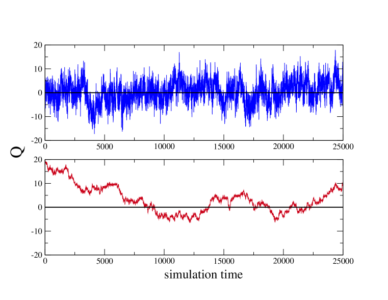
Figure 1: Trajectory history of topological charge ($Q$) versus simulation time at $\beta=6.59$ and lattice volume $48^{3}\times 96$ for open boundary condition (top) and periodic boundary condition (bottom). The data shown is at Wilson flow time $t/a^{2}=2$.

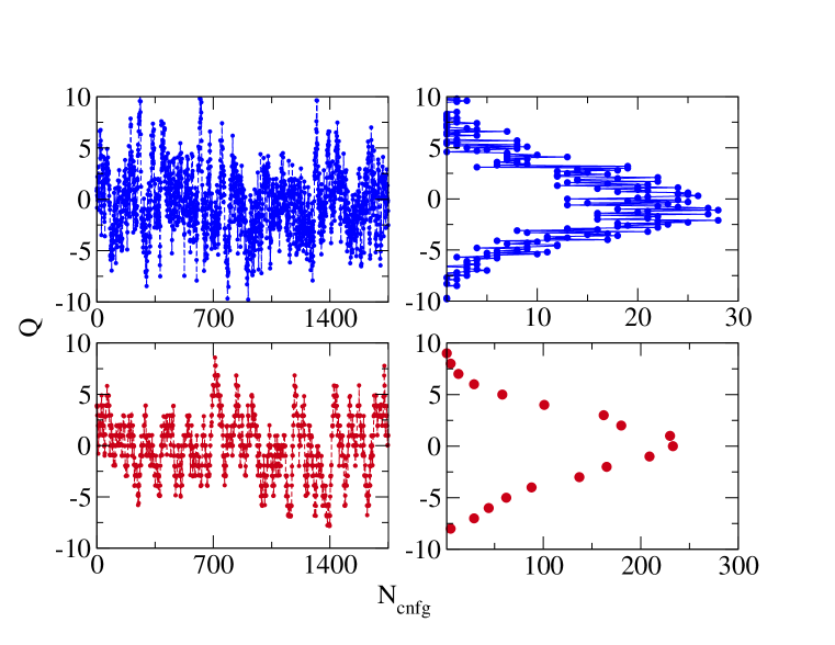
Figure 2: Distribution of $Q$ versus $N_{cnfg}$. Top one (blue) is open boundary condition and bottom (red) is periodic boundary condition at $\beta=6.42$ and lattice volume is $32^{3}\times 64$.

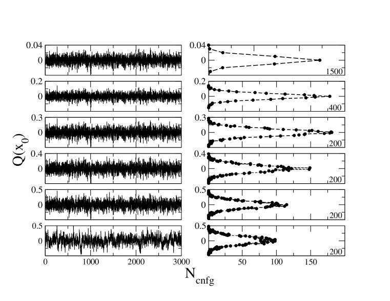
Figure 3: Distribution of $Q(x_{0})$ versus $N_{cnfg}$ for the ensemble $O_{2}$ where $x_{0}~{}=~{}0,~{}1,~{}2,~{}3,~{}4~{}{\rm and}~{}24$ from top to bottom respectively at $\beta=6.42$ and lattice volume $32^{3}\times 64$.

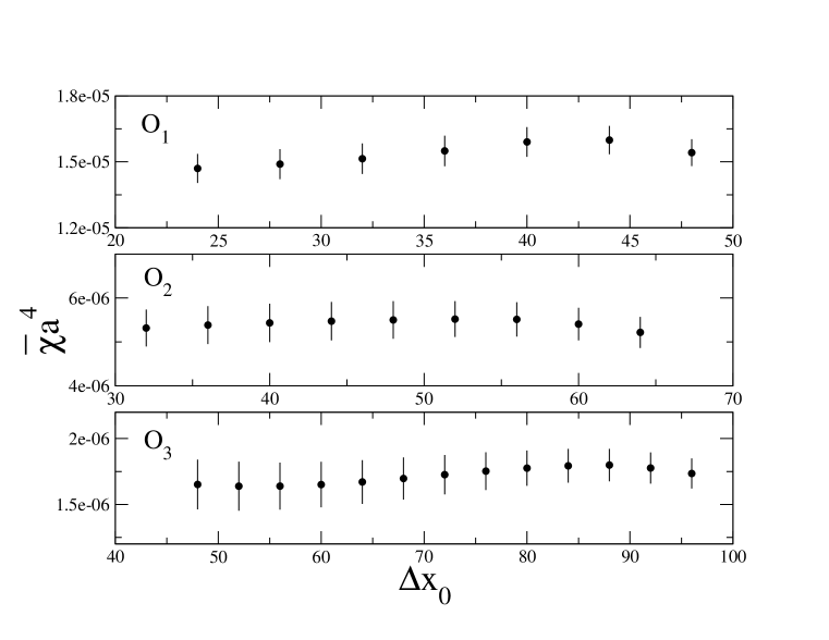
Figure 4: Subvolume susceptibility ($\overline{\chi}$) versus temporal length ($\Delta x_{0}$) for the ensembles $O_{1}$, $O_{2}$ and $O_{3}$.

Figure 5: Behaviour of topological susceptibility for both open and periodic boundary condition under Wilson flow plotted versus the flow time for different lattice spacings and lattice volumes.

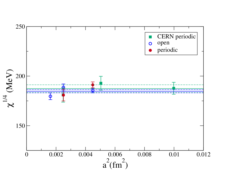
Figure 6: $\chi^{1/4}$ in dimensionful unit plotted versus $a^{2}$ for both open and periodic boundary condition for different lattice spacings and lattice volumes. For comparison, data from Ref.lspb for periodic boundary condition is also plotted. Also shown are the linear fits to the data Ref.lspb (green lines) and the data for open boundary condition (blue lines).

The open boundary condition has been proposed to help the tunneling of the system between different topological sectors characterized by the corresponding topological charge ($Q$) as one approaches the continuum limit. To that end we first compare the trajectory history of $Q$ for open versus periodic boundary conditions for a reasonably small lattice spacing. In figure 1 we plot the fluctuation of $Q$ versus simulation time at $\beta=6.59~{}(a=0.0402)$ and lattice volume $48^{3}\times 96$ for open boundary condition (top) and periodic boundary condition (bottom) both starting from random configurations. The data shown is at Wilson flow time $t/a^{2}=2$. Unless otherwise stated, all the data presented in the following are at the reference Wilson flow time ($t_{0}$). It is evident that with open boundary condition, thermalization is reached very fast whereas with periodic boundary condition it takes a long time just to reach thermalization. It is also evident that after thermalization, autocorrelation length is much larger for the periodic boundary condition compared to the open boundary condition. We have checked that the variation is not so marked for periodic boundary conditions at larger lattice spacings.

Next we look at the distribution of $Q$. In figure 2 along with time histories, we plot the histogram obtained for $Q$. Top one (blue) is open boundary condition and bottom (red) is periodic boundary condition at $\beta=6.42$ and lattice volume is $32^{3}\times 64$. We note that (1) as expected from the boundary conditions, top (blue) $Q$ is not an integer whereas for bottom (red), it is an integer and (2) even for this coupling ($\beta=6.42$) which is lower compared to figure 1, taking the same number of configurations, the top one gives much better spanning than the bottom. In the plot of histograms in this figure, we have used bin sizes of $0.1$ (top) and $1$ (bottom).

One needs to investigate the effect of open boundary condition on topological charge density ($q(x)$). We denote $q(x)$ integrated over the spatial volume at fixed Euclidean time $x_{0}$ by $Q(x_{0})$. The change in the behaviour of $Q(x_{0})$ as a function of time slice $x_{0}$ reveals the effect of open boundary in the temporal direction. The distribution of $Q(x_{0})$ versus $N_{cnfg}$ is presented in figure 3 for the ensemble $O_{2}$ where $x_{0}~{}=~{}0,~{}1,~{}2,~{}3,~{}4~{}{\rm and}~{}24$ from top to bottom respectively at $\beta=6.42$ and lattice volume $32^{3}\times 64$. The distribution of $Q(x_{0})$ is calculated with bin size of $0.01$. As we move from close to the boundary to deeper in the bulk, the spanning of $Q(x_{0})$ steadily increases and finally settles down in the bulk region. The same behaviour is also observed at the other end of the temporal lattice.

The topological susceptibility is defined as

$$\chi=\frac{\langle Q^{2}\rangle}{V}$$

where $V$ is the space-time volume. To investigate the effect of open boundary on susceptibility we define a subvolume susceptibility forcrand as follows:

$$\overline{\chi}\left(\Delta x_{0}\right)=\frac{\langle{\tilde{Q}}^{2}\rangle}{{\tilde{V}}}$$

where ${\tilde{Q}}$ is the $q(x)$ integrated over the spatial volume and temporal length ($\Delta x_{0}$) which is taken symmetrically over the mid point of the temporal direction. The subvolume ${\tilde{V}}$ is the product of spatial volume and $\Delta x_{0}$. In figure 4 we plot $\overline{\chi}$ versus $\Delta x_{0}$ for the ensembles $O_{1}$, $O_{2}$ and $O_{3}$. Due to open boundary in the temporal direction, there is slight dip close to the temporal boundary which is consistent with the behaviour of $Q(x_{0})$ as shown in figure 3. We find that, overall, the effect of the open boundary on the subvolume susceptibility is within the statistical uncertainties.

It is interesting to study the stability of $\chi$ with respect to Wilson flow time. In figure 5, we show the behaviour of $\chi$ for both open and periodic boundary condition under Wilson flow plotted versus the flow time for different lattice spacings and lattice volumes. For very early flow times, $\chi$ shows non-monotonous behaviour for both open and periodic boundary condition. For later flow times, $\chi$ converges from above to a plateau for open boundary condition whereas it converges from below for the periodic boundary condition. The values of susceptibility extracted at the reference flow time $t_{0}$ are given in table 2 and plotted in figure 6. In the figure 6, we show $\chi^{1/4}$ in dimensionful unit plotted against $a^{2}$ for both open and periodic boundary condition for different lattice spacings and volumes. We find that the results for open and periodic lattices are very close to each other at a given physical volume.

For comparison, data from Ref. lspb for periodic boundary condition is also plotted. Also shown are the linear fits to the data Ref. lspb (green lines) and the data for open boundary condition (blue lines). The extracted value of $\chi^{1/4}$ for the open boundary condition data is 184.7 (1.7) MeV which compares well with the result 187.4 (3.9) MeV of Ref. lspb .

Lattice	$a^{4}\chi/10^{-5}$	$\chi^{1/4}[{\rm MeV}]$
$O_{1}$	1.5418 (610)	185.4 (2.3)
$O_{2}$	0.5217 (354)	188.6 (3.5)
$O_{3}$	0.1794 (125)	179.6 (3.4)
$P_{1}$	1.7430 (973)	191.1 (3.0)
$P_{2}$	0.4407 (554)	180.8 (5.9)

Table 2: Topological susceptibility.

4 Conclusions

In this work we have shown that the open boundary condition in the temporal direction can yield the expected value of the topological susceptibility in lattice SU(3) Yang-Mills theory. The results agree with numerical simulations employing periodic boundary condition. The advantage of open boundary conditions over periodic boundary conditions (see, however, Ref. mm ) are illustrated in figure 1.

As further avenues of investigation, detailed comparison between Wilson flow and conventional smearing techniques used for smoothening gauge fields and the same between different algebraic as well as chirally improved fermionic definitions of topological charge density are in progress. It is also interesting to compute the topological charge density correlator (see Ref.topocorr and the references therein) using open boundary.

Acknowledgements Numerical calculations are carried out on the Cray XT5 and Cray XE6 systems supported by the 11th-12th Five Year Plan Projects of the Theory Division, SINP under the DAE, Govt. of India. We thank Richard Chang for the prompt maintenance of the systems and the help in data management. This work was in part based on the publicly available lattice gauge theory code openQCD openqcd .

References

- (1) M. Luscher, PoS LATTICE 2010, 015 (2010) [arXiv:1009.5877 [hep-lat]].
- (2) M. Luscher and S. Schaefer, JHEP 1107, 036 (2011) [arXiv:1105.4749 [hep-lat]].
- (3) M. Luscher and S. Schaefer, Comput. Phys. Commun. 184, 519 (2013) [arXiv:1206.2809 [hep-lat]].
- (4) M. Grady, arXiv:1104.3331 [hep-lat].
- (5) E. Witten, Nucl. Phys. B 156, 269 (1979).
- (6) G. Veneziano, Nucl. Phys. B 159, 213 (1979).
- (7) E. Seiler, Phys. Lett. B 525, 355 (2002) [hep-th/0111125].
- (8) L. Del Debbio, L. Giusti and C. Pica, Phys. Rev. Lett. 94, 032003 (2005) [hep-th/0407052].
- (9) S. Durr, Z. Fodor, C. Hoelbling and T. Kurth, JHEP 0704, 055 (2007) [hep-lat/0612021].
- (10) M. Luscher and F. Palombi, JHEP 1009, 110 (2010) [arXiv:1008.0732 [hep-lat]].
- (11) M. Luscher, Phys. Lett. B 593, 296 (2004) [hep-th/0404034].
- (12) L. Giusti and M. Luscher, JHEP 0903, 013 (2009) [arXiv:0812.3638 [hep-lat]].
- (13) H. Asakawa and M. Suzuki, J. Phys. A: Math. Gen. 29, 7811 (1996).
- (14) http://luscher.web.cern.ch/luscher/openQCD/
- (15) M. Guagnelli et al. [ALPHA Collaboration], Nucl. Phys. B 535, 389 (1998) [hep-lat/9806005].
- (16) S. Necco and R. Sommer, Nucl. Phys. B 622, 328 (2002) [hep-lat/0108008].
- (17) M. Luscher, Commun. Math. Phys. 293, 899 (2010) [arXiv:0907.5491 [hep-lat]].
- (18) M. Luscher, JHEP 1008, 071 (2010) [arXiv:1006.4518 [hep-lat]].
- (19) M. Luscher and P. Weisz, JHEP 1102, 051 (2011) [arXiv:1101.0963 [hep-th]].
- (20) S. Borsanyi, S. Durr, Z. Fodor, C. Hoelbling, S. D. Katz, S. Krieg, T. Kurth and L. Lellouch et al., JHEP 1209, 010 (2012) [arXiv:1203.4469 [hep-lat]].
- (21) P. de Forcrand, M. Garcia Perez, J. E. Hetrick, E. Laermann, J. F. Lagae and I. O. Stamatescu, Nucl. Phys. Proc. Suppl. 73, 578 (1999) [hep-lat/9810033].
- (22) G. McGlynn and R. D. Mawhinney, arXiv:1311.3695 [hep-lat].
- (23) A. Chowdhury, A. K. De, A. Harindranath, J. Maiti and S. Mondal, JHEP 1211, 029 (2012) [arXiv:1208.4235 [hep-lat]].