Lattice Boltzmann method for bosons and fermions and the fourth order Hermite polynomial expansion

Abstract

The Boltzmann equation with the Bhatnagar-Gross-Krook collision operator is considered for the Bose-Einstein and Fermi-Dirac equilibrium distribution functions. We show that the expansion of the microscopic velocity in terms of Hermite polynomials must be carried until the fourth order to correctly describe the energy equation. The viscosity and thermal coefficients, previously obtained by J.Y. Yang et al Shi20089389 ; PhysRevE.79.056708 through the Uehling-Uhlenbeck approach, are also derived here. Thus the construction of a lattice Boltzmann method for the quantum fluid is possible provided that the Bose-Einstein and Fermi-Dirac equilibrium distribution functions are expanded until fourth order in the Hermite polynomials.

I introduction

One of the greatest achievements of the Boltzmann equation gilberto is to determine the macroscopic hydrodynamical equations of a fluid from a phase space distribution function, $f(\boldsymbol{\chi},\boldsymbol{x},t)$, which describes the probability to find particles with microscopic velocity $\boldsymbol{\chi}$ in position $\boldsymbol{x}$ at time $t$. Nearly eighty years have passed since E. A. Uehling and G. E. Uhlenbeck PhysRev.43.552 solved the Boltzmann equation for the quantum fluid approximately by determining the small correction to the distribution function of non-interacting particles in case of a weak interaction. From this solution they derived the macroscopic hydrodynamical equations through the so-called Chapman-Enskog analysis and obtained the viscosity, $\eta$, and the thermal conductivity, $\kappa$, coefficients of the quantum fluid. The Uehling-Uhlenbeck approach was later revisited by T. Nikuni and A. Griffin nikuni98 who derived the macroscopic hydrodynamic equations, and the corresponding $\eta$ and $\kappa$ coefficients, of a trapped Bose gas above the Bose-Einstein condensation with damping. C. H. Lepienski and G. M. Kremer lepienski96 also determined these coefficients in case of specific two-body potentials, namely, Lennard-Jones and hard spheres. Recently the Boltzmann equation was found applicable to describe the collective oscillations of the two-dimensional Fermi gas PhysRevLett.108.070404 . All the above studies of the quantum fluid take the assumption of a two-body collision operator, as in the original Bolztmann equation. A simplifying assumption for the collision operator was introduced in the fifties by Bhatnagar-Gross-Krook (BGK) bgk54 , who considered it just as a simple drive to an equilibrium distribution function under a single relaxation time $\tau$. Nevertheless only recently the Uehling-Uhlenbeck approach was applied to solve the BGK-Boltzman equation for the quantum fluid Shi20089389 ; PhysRevE.79.056708 by J.Y. Yang et al., who derived its $\eta$ and $\kappa$ coefficients.

In the late eighties a numerical scheme was formulated to solve the Boltzmann equation with the BGK collision term succi ; sukop-thorne ; wolf-gladrow ; mohamad under the assumption of a discrete phase space where both the microscopic velocity and the position are restricted to a discrete set of values defined by a lattice. This method became widely known as the lattice Boltzmann method (LBM) and is used to simulate fluids with numerous advantages, such as easy implementation, inherent parallelization, and flexible treatment of the boundary conditions. The position space falls on a regular lattice where each point has a discrete set of microscopic velocity vectors that points towards a selected set of nearest nodes. To this discrete set of directions we associate the index $\alpha$, such that the microscopic velocities become $\boldsymbol{\chi}_{\alpha}$. The neighbor points are reached after a time $\Delta t$. The discreteness and rigidity of the microscopic velocity in the LBM makes the distribution function also become a discrete set, and instead of $f(\boldsymbol{\chi},\boldsymbol{x},t)$, one has $f_{\alpha}(\boldsymbol{x},t)$, fact that is of great numerical advantage. Then the lattice BGK-Boltzmann equation is derived from the continuous Boltzmann equation under a discretization procedure PhysRevE.56.6811,

$$f_{\alpha}(\boldsymbol{x}+\boldsymbol{\chi}_{\alpha}\Delta t,t+\Delta t)-f_{\alpha}(\boldsymbol{x},t)=$$

$$=-\frac{\Delta t}{\tau}\left[f_{\alpha}(\boldsymbol{x},t)-f_{\alpha}^{(0)}(\boldsymbol{x},t)\right],$$ (1)

which constantly drives the non-equilibrium distribution $f_{\alpha}(\boldsymbol{x},t)$ to the equilibrium distribution function $f_{\alpha}^{(0)}(\boldsymbol{x},t)$. Despite the tremendous success of the LBM method to describe the mass and momentum (Navier-Stokes) equations, the inclusion of a energy equation remained a challenge for sometime. The energy equation is needed to describe, for instance, the conversion of friction due to motion into heat, that increases the fluid temperature. This means that the transport of matter by particle diffusion is intertwined with the advected transport of enthalpy in such a way that the total energy is conserved for a closed system. The macroscopic hydrodynamical equations of the classical thermal compressible fluid are well-known, and can be derived from general macroscopic principles, as shown in the book of Landau & Lifshitz landau , for instance.

Many years after the development of the Uehling-Uhlenbeck approach, H. Grad grad49 ; PhysRevLett.78.243 devised another method to solve the continuous Boltzmann equation based on a sequence of approximations, obtained through the expansion of the distribution function in terms of the microscopic velocity space, expressed as a gaussian times a linear expansion in Hermite polynomials. Grad’s approach turned to be of paramount importance for the understanding of the properties of the LBM. For this reason the Hermite polynomial expansion method found a renewal of interest, such as in Refs. PhysRevLett.80.65, ; FLM:409537, . Despite the understanding brought by these references, the ingredients to describe the thermal compressible classical fluid were still missing, since the Hermite polynomial expansion was only carried there until third order ($N=3$), which is just insufficient. It was not until recently that the LBM for the thermal compressible fluid with a single BGK relaxation time, as described in Eq.(I), was derived. Philippi et al. (Ref. PhysRevE.73.056702, ), Siebert et al. (Ref. philippi07, ), and Shan and Chen (Ref. shan-chen07, ), succeeded to show that the thermal compressible properties of the classical fluid are correctly described if the Hermite polynomial expansion is carried until fourth order ($N=4$). Then the Chapman-Enskog analysis PhysRevE.73.056702 ; philippi07 ; shan-chen07 , applied to the BGK-Boltzmann equation with the Maxwell-Boltzmann equilibrium distribution function, gives the macroscopic hydrodynamical equations for the mass, momentum and energy balance, as obtained in the book of Landau & Lifshitz landau .

In this paper we apply the $N=4$ order Hermite polynomial expansion procedure to the quantum fluid and obtain its macroscopic hydrodynamical equations from a Chapman-Enskog analysis of the BGK-Boltzmann equation. We conclude that the construction of an LBM for the quantum fluid, similarly to the classical fluid, requires the Hermite polynomial expansion be carried until $N=4$ order to reach the correct energy equation, which besides the mass and momentum equations, is also needed for a full description of friction-heating processes. The coefficients $\eta$ and $\kappa$ of the BGK-Boltzmann quantum fluid, obtained through the Uehling-Uhlenbeck approach Shi20089389 ; PhysRevE.79.056708 , can only be retrieved in the $N=4$ order, and not in lowest order, as shown here. Therefore the halt of the Hermite polynomial expansion in $N=3$ order, as done in Ref. PhysRevE.79.056708, , impairs the derivation of the correct energy equation of the quantum fluid. Similarly the macroscopic hydrodynamical equations of Ref. yang10, do not correctly describe the energy balance equation because they are limited to $N=3$ order. Ref. PhysRevE.79.056708, provides the general form of the macroscopic hydrodynamical equations for the BGK-Boltzmann quantum fluid, but not the formulation of these equations in terms of the local macroscopic fields, namely, the chemical potential $\mu(\boldsymbol{x})$ (or the fugacity $z(\boldsymbol{x})$), the local temperature $\theta(\boldsymbol{x})$, and the local velocity $\boldsymbol{u}(\boldsymbol{x})$. In this paper we obtain the macroscopic hydrodynamical equation in terms of the above macroscopic variables.

We summarize the main achievements of this paper as follows. We obtain the equilibrium distribution function of the Bose-Einstein (BE) and Fermi-Dirac (FD) expanded until $N=4$ order in Hermite polynomials, namely, Eq.(III), or equivalently, Eq.(IV). We also obtain the Maxwell-Boltzmann (MB) equilibrium distribution function by Taylor expansion, namely, Eq.(B). In the classical limit the $N=4$ BE-FD equilibrium distribution function becomes the Taylor expanded MB equilibrium distribution function. All our results are obtained in $D$ dimensions, a feature that generalizes previous results discussed in the literature Shi20089389 ; PhysRevE.79.056708 . Next we derive the macroscopic hydrodynamical equations for the BE-FD cases, Eq.(21) and Eq.(II.3), and show that they become their MB counterparts, Eq.(5) and Eq.(6) in the classical limit, where BE, FD and MB statistics coincide. The viscosity and the thermal coefficients, given by Eq.(19) and Eq.(34), respectively, are the ones previously derived in Ref. Shi20089389, by another method. We show in Section VI that the $N=3$ Hermite expansion yields an incorrect energy equation and therefore this order is not suitable to describe either the classical or the quantum fluid. The $N=4$ order quantum fluid equations cannot be generally mapped into the classical ones for arbitrary fugacity, and only at the classical limit. However this mapping, as found in this paper, is always possible for the $N=3$. This shows, once again, that the $N=3$ order can not give a correct description of the quantum fluid. We find here an interesting property of the macroscopic hydrodynamical equations of the quantum fluid. To better understand this property we introduce the notation of pseudo variables, represented by a bar on the top of the corresponding variable. The property corresponds to the mapping of the pseudo variables into their counterparts, which leads the quantum into the classical equations. This mapping of the quantum into the classical equations is not complete though, as a single term in the heat flow term of the energy equation spoils it, as seen in Eq.(23). Finally we explicitly construct a LBM for the quantum fluids using the corresponding $N=4$ order LBM scheme and obtain some numerical results in the limit of dilute quantum fluids. In this dilute limit the BE and FD are small corrections to the MB statistics. Our numerical analysis is based on some two-dimensional lattices FLM:409537 ; PhysRevE.77.026707 , the so-called d2q17 and d2q37 lattices. Thus we are able to check that indeed quantum fluid motion generates friction and the heat created results into a temperature change such that the total energy remains conserved during a time evolution process. Our numerical study is restricted to an adiabatic process as there is no external contact or force. We treat a two-dimensional system under periodic boundary conditions, thus without external borders and with no external applied force, just an initial displacement from equilibrium set by the initial conditions.

The paper is organized as follows. In section II we review the classical macroscopic hydrodynamical equations as described by Landau & Lifshitz’s landau and also those obtained from a Chapman-Enskog analysis of the $N=4$ order Hermite polynomial expansion PhysRevE.73.056702 ; philippi07 ; shan-chen07 . We also present in section II the macroscopic hydrodynamical equations of the quantum fluids and discuss several of their aspects, such as the introduction of the pseudo variables and the viscosity and thermal coefficients. The dimensionless units are also introduced in section II. In the next section III the Hermite polynomial decomposition is performed on the BE and FD equilibrium distribution functions. The derivation of the MB equilibrium distribution function by Taylor expansion is left for the appendix B. Some properties of the Hermite polynomials are discussed in appendix A. The passage from the continuum to the discrete through the Gauss-Hermite quadrature is the subject of section IV. The Chapman-Enskog analysis is performed in section V and the relations required to determine several tensors are listed in the appendix D. To obtain the macroscopic hydrodynamical equations one needs some position and time cross derivative terms derived in appendix C. In section VI we obtain a no go theorem for the Hermite polynomial expansion to order $N=3$. The dilute quantum fluid is treated in section VII and numerical results in this limit are studied in section VIII.

There has been in the past years attempts to construct a LBM for the classical thermal compressible fluid starting from ad hoc assumptions of the equilibrium distribution function PhysRevE.47.R2249 ; qian93 ; PhysRevE.50.2776 ; wolf-gladrow ; PhysRevE.76.016702 . This approach was never attempted for the quantum fluid.

II Macroscopic equations for classical and quantum fluids

In this section we present the macroscopic hydrodynamical equations of the quantum fluid obtained in this paper through the $N=4$ Hermite polynomial expansion of the BE and FD equilibrium distribution functions. We express them almost entirely in terms of the pseudo variables, with the exception of a single term in the heat flow. From these equations we obtain the thermal coefficients, and the classical MB limit. The actual derivation of these equations is done in sections III and V, with the help of appendices D and C. In order to best convey our results we review the derivation of the macroscopic hydrodynamical equations for the classical fluid, both from the point of view of the macroscopic principles and of the N=4 Hermite polynomial expansion of the Maxwell-Boltzmann equilibrium distribution function PhysRevE.73.056702 ; philippi07 ; shan-chen07 . Thus the first two subsections are reviews while the last one contains our original results.

II.1 Derivation of the macroscopic equation from general principles

For the ideal fluid (no viscosity) the equations describing the conservation of mass, momentum and energy follow straightforwardly from general macroscopic principles of thermodynamics and newtonian mechanics, as well described, for instance, in the book of Landau & Lifshitz landau . For the conservation of mass one obtains that

$$\frac{\partial\rho}{\partial t}+\frac{\partial}{\partial x^{i}}(\rho u^{i})=0.$$ (2)

For the conservation of momentum one obtains Euler’s equation,

$$\frac{\partial\rho u^{i}}{\partial t}+\frac{\partial}{\partial x^{j}}(p\delta^{ij}+\rho u^{i}u^{j})=0,$$ (3)

and the law of conservation of energy is

$$\frac{\partial\left(\rho\boldsymbol{u}^{2}/2+\rho\varepsilon\right)}{\partial t}+\frac{\partial}{\partial x^{j}}[u^{j}(\rho\boldsymbol{u}^{2}/2+\rho\varpi)]=0,$$ (4)

where $p$, $\varepsilon$ and $\varpi$ describe the pressure, the internal energy and the enthalpy of the fluid, $\varpi\equiv\varepsilon+p/\rho$. These equations describe the time evolution of the density, $\rho$, the macroscopic velocity, $u^{i}$, and the local temperature, $\theta$, in some reduced units, which are explained in this paper. The presence of viscosity and thermal conduction in a fluid changes the equations for momentum and energy, which become

$$\frac{\partial(\rho u^{i})}{\partial t}+\frac{\partial}{\partial x^{j}}\left(p\delta^{ij}+\rho u^{i}u^{j}-\sigma^{ij}\right)=0,$$ (5)

and

$$\frac{\partial\left(\rho\boldsymbol{u}^{2}/2+\rho\varepsilon\right)}{\partial t}+\frac{\partial}{\partial x^{j}}\left[u^{j}\left(\rho\boldsymbol{u}^{2}/2+\rho\varpi\right)+\right.$$

$$\left.+Q^{j}-u^{k}\sigma^{jk}\right]=0,$$ (6)

respectively. The momentum flux tensor becomes $p\delta^{ij}+\rho u^{i}u^{j}-\sigma^{ij}$, thus is changed by the presence of the viscosity stress tensor,

$$\sigma^{ij}=\eta\left(\frac{\partial u^{i}}{\partial x^{j}}+\frac{\partial u^{j}}{\partial x^{i}}-\frac{2}{D}\delta^{ij}\frac{\partial u^{l}}{\partial x^{l}}\right)+\zeta\delta^{ij}\frac{\partial u^{l}}{\partial x^{l}}$$ (7)

where $\eta$ and $\zeta$ being the dynamic and volumetric viscosities, respectively, and $D$ the number of space dimensions. Similarly, the total energy flux becomes $u^{j}(\rho\boldsymbol{u}^{2}/2+\rho\varpi)+Q^{j}-u^{k}\sigma^{jk}$, where

$$Q^{j}=-\kappa\frac{\partial\theta}{\partial x^{j}}$$ (8)

is the heat flux flow due to thermal conduction, and $\kappa$ is the thermal conductivity. The presence of viscosity introduces irreversible transfer of momentum within the fluid and Eq.(5) is essentially the Navier-Stokes equation. From the other side notice that Eq.(6) shows that in a viscous fluid the friction that stems from the loss of momentum results into an increase of temperature thus conserving the total energy in the process.

For the sake of completeness we express the equations for momentum and energy in a different fashion. obtained by simple manipulation of Eqs. (2), (5) and (6). The resulting equations are expressed in terms of the stress tensor

$$P^{i\,j}\equiv\rho\theta\delta^{i\,j}-\sigma^{i\,j}.$$ (9)

The momentum conservation equation becomes,

$$\rho\left(\frac{\partial}{\partial t}+u^{j}\frac{\partial}{\partial x^{j}}\right)u^{i}+\frac{\partial}{\partial x^{j}}P^{i\,j}=0.$$ (10)

The energy conservation equation becomes,

$$\frac{\partial}{\partial t}\left(\frac{D}{2}\rho\theta\right)+\frac{\partial}{\partial x^{j}}\left(\frac{D}{2}\rho\theta u^{j}\right)+$$

$$+\frac{1}{2}\left(\frac{\partial u^{i}}{\partial x^{j}}+\frac{\partial u^{j}}{\partial x^{i}}\right)P^{i\,j}+\frac{\partial}{\partial x^{i}}Q^{i}=0.$$ (11)

II.2 Macroscopic equations from the Maxwell-Boltzmann distribution function

The Hermite polynomial expansion of the Maxwell-Boltzmann equilibrium distribution function carried until $N=4$ order PhysRevE.73.056702 ; philippi07 ; shan-chen07 , and the subsequent Chapman-Enskog analysis applied to the BGK-Boltzmann equation, exactly reproduce the above equations obtained by general macroscopic principles. Thus the equations for the density, Eq.(2), the macroscopic velocity, Eq.(5), and the temperature, Eq.(6) also hold here, and so do Eq(10) and Eq.(II.1). However thermodynamic functions and coefficients acquire special features. The viscosity stress tensor has a null volumetric viscosity ($\zeta=0$), and the dynamic viscosity is given by,

$$\eta\equiv\rho\theta\tau\left(1-\frac{\Delta t}{2\tau}\right),$$ (12)

and the thermal conductivity by,

$$\kappa\equiv\left(\frac{D+2}{2}\right)\rho\theta\tau\left(1-\frac{\Delta t}{2\tau}\right).$$ (13)

such that $\kappa/\eta=(D+2)/2$. Notice that these coefficients are local because of their $\theta$ and $\rho$ dependence. The pressure is $p=\rho\,\theta$, the internal energy is, $\varepsilon\equiv D\theta/2$, such that the enthalpy becomes , $\varpi\equiv(D+2)\theta/2$.

II.3 Macroscopic equations from the Bose-Einstein and Fermi-Dirac distribution functions

The $N=4$ Hermite polynomial expansion of the BE and FD equilibrium distribution functions, followed by the Chapman-Enskog analysis done in the BGK-Boltzmann equation, leads to the macroscopic hydrodynamical equations for the quantum fluid in terms of the temperature $\theta$, the velocity $u^{i}$, and the chemical potential $\mu$. The fugacity can be used instead of the chemical potential, and is defined as,

$$z\equiv e^{\frac{\mu}{\theta}}.$$ (14)

We find that the quantum equations are very similar to the classical ones, provided that some auxiliary variables are introduced, starting with the pseudo-temperature defined below.

$$\bar{\theta}=\theta\frac{g_{\frac{D}{2}+1}(z)}{g_{\frac{D}{2}}(z)}$$ (15)

where,

$$g_{\nu}(z)\equiv\frac{1}{\Gamma(\nu)}\int^{\infty}_{0}\frac{x^{\nu-1}\,dx}{z^{-1}e^{x}\pm 1}.$$ (16)

The $+$ and $-$ signs in the denominator correspond to FD and BE statistics, respectively. Indeed the MB limit is retrieved from the FD and MB statistics in the limit that $z^{-1}e^{x}\pm 1\approx z^{-1}e^{x}$, thus the term $\pm 1$ becomes irrelevant in the denominator. Since $\Gamma(\nu)=\int^{\infty}_{0}e^{-x}x^{\nu-1}\,dx$, one obtains that $g_{\nu}(z)=z$ for the MB limit. Thus we conclude that in the classical limit the pseudo-temperature is the temperature itself. The BE-FD density is not an independent parameter, as in the MB case, but a function of the the temperature $\theta$ and the fugacity $z$,

$$\rho=(2\pi\theta)^{\frac{D}{2}}g_{\frac{D}{2}}(z).$$ (17)

Based on the above definitions of $\rho$ and $\bar{\theta}$ we introduce the pseudo viscosity stress tensor

$${\bar{\sigma}}^{ij}\equiv\bar{\eta}\left(\frac{\partial u^{i}}{\partial x^{j}}+\frac{\partial u^{j}}{\partial x^{i}}-\frac{2}{D}\delta^{ij}\right),$$ (18)

which depends on the pseudo dynamic viscosity defined as,

$$\bar{\eta}\equiv\rho\bar{\theta}\tau\left(1-\frac{\Delta t}{2\tau}\right).$$ (19)

We also define the pseudo thermal conductivity,

$$\bar{\kappa}\equiv\frac{D+2}{2}\rho\bar{\theta}\tau\left(1-\frac{\Delta t}{2\tau}\right).$$ (20)

Their ratio is constant, $\bar{\kappa}/\bar{\eta}=(D+2)/2$, meaning that, like in the MB case, thermal and mechanical transfers are done by the same distribution and at the same rate, as there is only one BGK time relaxation parameter.

The conservation of mass is given by Eq.(2) and the momentum balance equation for quantum fluids is described by,

$$\frac{\partial}{\partial t}(\rho u^{i})+\frac{\partial}{\partial x^{j}}\left[\rho\left(\bar{\theta}\delta^{ij}+u^{i}u^{j}\right)\right]-\frac{\partial{\bar{\sigma}}^{ij}}{\partial x^{j}}=0$$ (21)

Comparison between Eq.(5) and Eq.(21) shows that the classical and the quantum equations are the same provided that the true temperature $\theta$ is mapped into the pseudo temperature, $\bar{\theta}$. The same does not hold for the energy equations, namely, Eq.(6) and Eq.(II.3), as the dependence of the quantum case in the true temperature cannot collapse into the pseudo temperature. The fugacity $z$ explicitly appears there through the function $g(z)$, as seen below.

$$\frac{\partial}{\partial t}\left(\frac{\rho}{2}\boldsymbol{u}^{2}+\frac{\rho}{2}D\bar{\theta}\right)+\frac{\partial}{\partial x^{j}}\left[\left(\frac{\rho}{2}\boldsymbol{u}^{2}+\frac{\rho}{2}\bar{\theta}(D+2)\right)u^{j}+\right.$$

$$\left.+{\tilde{Q}}^{j}-u^{k}{\bar{\sigma}}^{j\,k}\right]=0,$$ (22)

where the true heat flux vector is given by,

$${\tilde{Q}}^{j}={\bar{Q}}^{j}-\frac{\partial}{\partial x^{j}}\left[\bar{\kappa}\left(g(z)-1\right)\bar{\theta}\right],\,{\bar{Q}}^{j}\equiv-\bar{\kappa}\frac{\partial}{\partial x^{i}}\bar{\theta}.$$ (23)

Thus the writing of the energy equation solely in terms of pseudo variables is spoiled just by the extra term, that must be added to the pseudo heat flux vector, ${\bar{Q}}^{j}$, to obtain the true one, ${\tilde{Q}}^{j}$. The function $g(z)$ is defined as,

$$g(z)\equiv\frac{g_{\frac{D}{2}}(z)\cdot g_{\frac{D}{2}+2}(z)}{\left(g_{\frac{D}{2}+1}(z)\right)^{2}}.$$ (24)

In conclusion we find remarkable that the replacement of ${\tilde{Q}}^{j}$ by ${\bar{Q}}^{j}$ in Eq.(II.3) renders the mass, momentum and energy equations for the quantum and classical fluids formally identical, provided that the density and the temperature are replaced by Eqs.(17) and (15), respectively. Another way to see this connection is by noticing that for the quantum problem all the explicit and linear dependence in the temperature appears through the pseudo temperature. This is the reason why the mass and momentum equations of quantum and classical cases are formally equivalent, but not the energy equation. The quantum energy equation has an extra quadratic dependence on the temperature brought by the function $g(z)-1$, as discussed in the coming sections. There is a link between this quadratic behavior in the temperature and the $g(z)$ function, as shown by the identity below.

$$\theta^{2}\frac{g_{\frac{D}{2}+2}(z)}{g_{\frac{D}{2}}(z)}={\bar{\theta}}^{2}g(z).$$ (25)

The quantum counterparts of the classical momentum and energy equations, namely, Eqs.(10) and (II.1), are given by

$$\rho\left(\frac{\partial}{\partial t}+u^{j}\frac{\partial}{\partial x^{j}}\right)u^{i}+\frac{\partial}{\partial x^{j}}{\bar{P}}^{i\,j}=0,$$ (26)

and,

$$\frac{\partial}{\partial t}\left(\frac{D}{2}\rho\bar{\theta}\right)+\frac{\partial}{\partial x^{j}}\left(\frac{D}{2}\rho\bar{\theta}u^{j}\right)+$$

$$+\frac{1}{2}\left(\frac{\partial u^{i}}{\partial x^{j}}+\frac{\partial u^{j}}{\partial x^{i}}\right){\bar{P}}^{i\,j}+\frac{\partial}{\partial x^{i}}{\tilde{Q}}^{i}=0,$$ (27)

respectively. We also define the pseudo stress tensor,

$${\bar{P}}^{i\,j}\equiv\rho\bar{\theta}\delta^{i\,j}-\bar{\sigma}^{i\,j}.$$ (28)

We obtain the true thermal conductivity coefficient, $\kappa_{\theta}$, and the chemical potential coefficient, $\kappa_{\mu}$, through their definition:

$${\tilde{Q}}^{j}=-\kappa_{\theta}\frac{\partial\theta}{\partial x^{j}}-\kappa_{\mu}\frac{\partial\mu}{\partial x^{j}}.$$ (29)

To derive the above coefficients, we write the pseudo heat flux vector as,

$${\tilde{Q}}^{j}=\bar{\theta}\frac{\partial\bar{\kappa}}{\partial x^{j}}-\frac{\partial}{\partial x^{j}}\left[\bar{\kappa}g(z)\bar{\theta}\right].$$ (30)

Firstly derive the function $g_{\mu}(z)$ of Eq.(16):

$$\frac{\partial g_{\mu}(z)}{\partial x^{j}}=g_{\mu-1}(z)\left(-\frac{\mu}{\theta}\frac{\partial\theta^{2}}{\partial x^{j}}+\frac{1}{\theta}\frac{\partial\mu}{\partial x^{j}}\right),$$ (31)

which leads to,

$$\frac{\partial\bar{\kappa}}{\partial x^{j}}=\rho\tau^{\prime}\left\{\left[\left(\frac{D}{2}+1\right)\frac{g_{\frac{D}{2}+1}(z)}{g_{\frac{D}{2}}(z)}-\frac{\mu}{\theta}\right]\frac{\partial\theta}{\partial x^{j}}+\frac{\partial\mu}{\partial x^{j}}\right\},$$

where $\tau^{\prime}\equiv(D/2+1)\tau(1-\Delta t/2\tau)$. One also obtains that,

$$\frac{\partial\left(\bar{\kappa}\bar{\theta}g(z)\right)}{\partial x^{j}}=\rho\tau^{\prime}\left\{\left[\left(\frac{D}{2}+2\right)\theta\frac{g_{\frac{D}{2}+2}(z)}{g_{\frac{D}{2}}(z)}-\mu\frac{g_{\frac{D}{2}+1}(z)}{g_{\frac{D}{2}}(z)}\right]\cdot\right.$$

$$\left.\cdot\frac{\partial\theta}{\partial x^{j}}+\theta\frac{g_{\frac{D}{2}+1}(z)}{g_{\frac{D}{2}}(z)}\frac{\partial\mu}{\partial x^{j}}\right\}.$$ (33)

The last two equations are introduced in Eq.(30) to obtain the coefficients $\kappa_{\theta}$ and $\kappa_{\mu}$:

$$\kappa_{\theta}=\kappa\left[\left(\frac{D}{2}+2\right)\frac{g_{\frac{D}{2}+2}(z)}{g_{\frac{D}{2}+1}(z)}-\left(\frac{D}{2}+1\right)\frac{g_{\frac{D}{2}+1}(z)}{g_{\frac{D}{2}}(z)}\right]$$

(34)

$$\kappa_{\mu}=0,$$ (35)

where $\kappa$ is the MB (classical) thermal conductivity, given by Eq.(13). These are the coefficients obtained in Ref. Shi20089389, for the BGK-Boltzmann equation using the Uehling-Uhlenbeck approach.

III Expansion of the quantum equilibrium distribution functions by Hermite polynomials to $N=4$ order

Here we expand the quantum equilibrium distribution functions until $N=4$ order of Hermite polynomials. Consider the BE and FD distribution functions, given by,

$$f^{(0)}(\boldsymbol{\chi})=\frac{1}{\exp\left[\frac{\left(\boldsymbol{\chi}-\boldsymbol{v}\right)^{2}m}{2k_{B}T}-\frac{\mu^{\prime}}{k_{B}T}\right]\pm 1},$$ (36)

which depend on the microscopic velocity $\boldsymbol{\chi}$ and other three locally defined quantities, namely, the temperature $T(\boldsymbol{x})$, the macroscopic velocity $\boldsymbol{v}(\boldsymbol{x})$ and the chemical potential $\mu^{\prime}(\boldsymbol{x})$.

We define the following dimensionless quantities, based on a reference temperature $T_{r}$, and a reference velocity:

$$c_{r}\equiv\sqrt{\frac{kT_{r}}{m}},$$ (37)

both not present in the original BE-FD equilibrium distribution functions. Then the dimensionless temperature is

$$\theta\equiv\frac{T}{T_{r}},$$ (38)

and the microscopic and macroscopic dimensionless velocities are defined as

$$\boldsymbol{\xi}\equiv\frac{\boldsymbol{\chi}}{c_{r}},\,\,\mbox{and}$$ (39)

$$\boldsymbol{u}\equiv\frac{\boldsymbol{v}}{c_{r}}.$$ (40)

The dimensionless chemical potential is,

$$\mu\equiv\frac{\mu^{\prime}}{k_{B}T_{r}},$$ (41)

and the fugacity can be expressed in two ways,

$$z\equiv e^{\frac{\mu^{\prime}}{k_{B}T}}=e^{\frac{\mu}{\theta}}.$$ (42)

The BE-FD function expressed in terms of dimensionless parameters becomes,

$$f^{(0)}(\boldsymbol{\xi})=\frac{1}{z^{-1}\exp\left[\frac{\left(\boldsymbol{\xi}-\boldsymbol{u}\right)^{2}}{2\theta}\right]\pm 1}.$$ (43)

The first three moments of the BE-FD function, obtained by integrating over the microscopic velocity $\boldsymbol{\chi}$, give that,

$$n(\boldsymbol{x})=m\left(\frac{m}{2\pi\hbar}\right)^{D}\int d^{D}\boldsymbol{\chi}\;f^{0}(\boldsymbol{\chi}),$$ (44)

$$\boldsymbol{v}(\boldsymbol{x})=\frac{1}{\rho(\boldsymbol{x})}\int d^{D}\boldsymbol{\chi}\;\boldsymbol{\chi}f^{0}(\boldsymbol{\chi}),\,\mbox{and}$$ (45)

$$\frac{D}{2}k_{B}\bar{T}(\boldsymbol{x})=\frac{1}{\rho(\boldsymbol{x})}\int d^{D}\boldsymbol{\chi}\;\frac{1}{2}m\left[\boldsymbol{\chi}-\boldsymbol{v}(\boldsymbol{x})\right]^{2}f^{0}(\boldsymbol{\chi}).$$ (46)

We define the pseudo temperature $\bar{T}$ because the third moment is the internal energy, $\varepsilon=Dk_{B}\bar{T}/2$, and in the classical case we know that $\bar{T}=T$. Notice that the density $n$ has the dimension of a $D$ dimensional space density, as expected, namely, of $mass/(length)^{D}$, because $mv/2\pi\hbar$ has the dimension of $length^{-1}$. Thus through the following constant, which has the dimension of density,

$$n_{0}\equiv m\left(\frac{mc_{r}}{2\pi\hbar}\right)^{D}.$$ (47)

By taking averages over the quantum equilibrium distribution function we obtain the dimensionless density $\rho$ of Eq.(17), the macroscopic velocity $\boldsymbol{u}$, and the pseudo-temperature $\bar{\theta}$ of Eq.(15):

$$\rho(\boldsymbol{x})\equiv\frac{n(\boldsymbol{x})}{n_{0}}=\int d^{D}\boldsymbol{\xi}\;f^{(0)}(\boldsymbol{\xi}),$$ (48)

$$\boldsymbol{u}(\boldsymbol{x})=\frac{1}{\rho(\boldsymbol{x})}\int d^{D}\boldsymbol{\xi}\;\boldsymbol{\xi}f^{(0)}(\boldsymbol{\xi}),\,\mbox{and}$$ (49)

$$\frac{D}{2}\bar{\theta}(\boldsymbol{x})=\frac{1}{\rho(\boldsymbol{x})}\int d^{D}\boldsymbol{\xi}\;\frac{1}{2}\left[\boldsymbol{\xi}-\boldsymbol{u}(\boldsymbol{x})\right]^{2}f^{(0)}(\boldsymbol{\xi}).$$ (50)

The explicit calculation of these moments are done below.

The N${}^{\mbox{th}}$ order Hermite polynomial is defined by the Rodrigues’ formula,

$$H^{i_{1}i_{2}...i_{N}}(\boldsymbol{\xi})=\frac{(-1)^{N}}{\omega(\boldsymbol{\xi})}\frac{\partial^{N}\omega(\boldsymbol{\xi})}{\partial\xi^{i_{1}}\xi^{i_{2}}...\xi^{i_{N}}},$$ (51)

where,

$$\omega(\boldsymbol{\xi})\equiv\frac{1}{(2\pi)^{\frac{D}{2}}}\exp{\left(-\frac{\boldsymbol{\xi}^{2}}{2}\right)},$$ (52)

is the gaussian function. The orthonormality of the Hermite polynomials, $H^{i_{1}i_{2}...i_{N}}(\boldsymbol{\xi})$, is given by,

$$\int d^{D}\boldsymbol{\xi}\,\omega(\boldsymbol{\xi})H^{i_{1}i_{2}...i_{N}}(\boldsymbol{\xi})H^{j_{1}j_{2}...j_{M}}(\boldsymbol{\xi})=$$ (53)

$$=\delta^{NM}(\delta^{i_{1}j_{1}}\delta^{i_{2}j_{2}}...\delta^{i_{N}j_{N}}+\mbox{all permutations of j's}).$$

We seek the decomposition of the BE-FD function $f^{(0)}$ of Eq.(43) in powers of Hermite polynomials.

$$f^{(0)}(\boldsymbol{x},\boldsymbol{\xi})=\omega(\boldsymbol{\xi})\sum^{\infty}_{N=0}\frac{1}{N!}a^{i_{1}i_{2}...i_{N}}(\boldsymbol{x})H^{i_{1}i_{2}...i_{N}}(\boldsymbol{\xi}).$$ (54)

Notice that this decomposition splits the dependence on the dimensionless microscopic velocity, which falls in the Hermite polynomials, from the other variables, since the coefficients of this expansion carry all the information about the local macroscopic fields. For this reason the following notation is employed, $a^{i_{1}\,i_{2}...i_{N}}(\boldsymbol{x})\equiv a^{i_{1}\,i_{2}...i_{N}}[z(\boldsymbol{x}),\boldsymbol{u}(\boldsymbol{x}),\theta(\boldsymbol{x})]$. Applying the orthonormality of the Hermite polynomials one obtains an expression for the coefficients:

$$a^{i_{1}i_{2}...i_{N}}(\boldsymbol{x})=\int f^{(0)}(\boldsymbol{x},\boldsymbol{\xi})H^{i_{1}i_{2}...i_{N}}(\boldsymbol{\xi})d^{D}\boldsymbol{\xi}$$ (55)

More details about properties of the Hermite polynomials are given in Appendix A. Notice that the BE-FD function is even in the difference between the macroscopic and the microscopic velocities, $f^{(0)}(\boldsymbol{x},\boldsymbol{\xi-u})=f^{(0)}(\boldsymbol{x},\boldsymbol{u-\xi})$, a helpful property to compute the coefficients of Eq.(55). Then the coefficient associated to any odd Hermite polynomial vanishes since $\int d^{D}\boldsymbol{\xi}\,f(\boldsymbol{\xi-u})H^{i_{1}\ldots i_{2L+1}}(\boldsymbol{\xi-u})=0$. A discussion of such properties is done in the appendix A. We introduce the variable $\boldsymbol{\eta}=\boldsymbol{\xi}-\boldsymbol{u}$ and write the BE-FD distribution function as $f(\boldsymbol{\eta})=1/\left(z^{-1}e^{\frac{\eta^{2}}{2\theta}}\pm 1\right)$ to express the coefficients as,

$$a^{i_{1}i_{2}...i_{N}}=\int f^{(0)}(\boldsymbol{\eta})H^{i_{1}i_{2}...i_{N}}(\boldsymbol{\xi})d^{D}\boldsymbol{\eta}.$$ (56)

Coefficient N=0 - The integration over a spherical shell in D dimensions is $d^{D}\boldsymbol{\eta}=\frac{D\pi^{\frac{D}{2}}}{\Gamma\left(\frac{D}{2}+1\right)}\eta^{D-1}d\eta$ and the lowest Hermite coefficient becomes,

$$a=\int\frac{Hd^{D}\boldsymbol{\eta}}{z^{-1}e^{\frac{\eta^{2}}{2\theta}}\pm 1}=\frac{D\pi^{\frac{D}{2}}}{\Gamma\left(\frac{D}{2}\pm 1\right)}\int^{\infty}_{0}\frac{\eta^{D-1}d\eta}{z^{-1}e^{\frac{\eta^{2}}{2\theta}}\pm 1}.$$ (57)

since $H=1$. Defining $x=\eta^{2}/2\theta$, one obtains that,

$$a=(2\pi)^{\frac{D}{2}}\theta^{\frac{D}{2}}g_{\frac{D}{2}}(z)$$ (58)

where in the last line we have introduced the function $g_{\nu}(z)$ of Eq.(16). This coefficient is the density itself, $a=\rho=\int d^{D}\boldsymbol{\xi}\;f^{(0)}(\boldsymbol{\xi})$, as given by Eq.(17).

Coefficient N=1 - To obtain this coefficient take Eq.(173) such that,

$$a^{i}=\int f^{(0)}(\boldsymbol{\eta})H^{i}(\boldsymbol{\xi})d^{D}\boldsymbol{\eta}=$$

$$=\int f^{(0)}(\boldsymbol{\eta})\left[H^{i}(\boldsymbol{\eta})+Hu^{i}\right]d^{D}\boldsymbol{\eta}=u^{i}\int f^{(0)}(\boldsymbol{\eta})d^{D}\boldsymbol{\eta}=$$

$$=u^{i}\rho$$ (59)

as the first integral vanishes because it is odd. Using analogous arguments, we find the next coefficients.

Coefficient N=2 - One gets from Eq.(174) that,

$$a^{ij}=\int f^{(0)}(\boldsymbol{\eta})H^{ij}(\boldsymbol{\xi})d^{D}\boldsymbol{\eta}=\int f^{(0)}(\boldsymbol{\eta})\left[H^{ij}(\boldsymbol{\eta})+\right.$$

$$\left.+u^{i}H^{j}(\boldsymbol{\eta})+u^{j}H^{i}(\boldsymbol{\eta})+u^{i}u^{j}H\right]d^{D}\boldsymbol{\eta}=$$

$$=\int f^{(0)}(\boldsymbol{\eta})H^{ij}(\boldsymbol{\eta})d^{D}\boldsymbol{\eta}+\rho u^{i}u^{j}.$$ (60)

The terms proportional to $u^{j}$ vanish because of the odd integrals and it remains to calculate the integrals below.

$$\int f^{(0)}(\boldsymbol{\eta})\eta^{i}\eta^{j}d^{D}\boldsymbol{\eta}=\frac{\delta^{ij}}{D}\int f^{(0)}(\boldsymbol{\eta})\eta^{2}d^{D}\boldsymbol{\eta}=$$

$$=\theta\rho\frac{g_{\frac{D}{2}+1}(z)}{g_{\frac{D}{2}}(z)}\delta^{ij}.$$ (61)

The other integral to compute is,

$$\int f^{(0)}(\boldsymbol{\eta})H^{ij}(\boldsymbol{\eta})d^{D}\boldsymbol{\eta}=\rho\delta^{ij}\left(\theta\frac{g_{\frac{D}{2}+1}(z)}{g_{\frac{D}{2}}(z)}-1\right).$$ (62)

Introducing the pseudo temperature of Eq.(15), the second order coefficient becomes,

$$a^{ij}=\rho\left[\delta^{ij}\left(\bar{\theta}-1\right)+u^{i}u^{j}\right].$$ (63)

Hereafter we directly use Eq.(15) to shorten the notation.
Coefficient N=3 - One gets from Eq.(175) that,

$$a^{ijk}=\int f^{(0)}(\boldsymbol{\eta})H^{ijk}(\boldsymbol{\xi})d^{D}\boldsymbol{\eta}=$$

$$=\int f^{(0)}(\boldsymbol{\eta})\left[H^{ijk}(\boldsymbol{\eta})+u^{i}H^{jk}(\boldsymbol{\eta})+u^{j}H^{ik}(\boldsymbol{\eta})+u^{k}H^{ij}(\boldsymbol{\eta})+\right.$$

$$\left.+u^{i}u^{j}H^{k}(\boldsymbol{\eta})+u^{i}u^{k}H^{j}(\boldsymbol{\eta})+u^{j}u^{k}H^{i}(\boldsymbol{\eta})+u^{i}u^{j}u^{k}H\right]d^{D}\boldsymbol{\eta}=$$

$$=\rho\left[(u^{i}\delta^{jk}+u^{j}\delta^{ik}+u^{k}\delta^{ij})\bar{\theta}+u^{i}u^{j}u^{k}\right].$$

Terms proportional to $u^{i}u^{j}$ vanish because they are proportional to integrals over a Hermite polynomial of odd order.

Coefficient N=4 - One gets from Eq.(176) that,

$$a^{ijkl}=\int f^{(0)}(\boldsymbol{\eta})H^{ijkl}(\boldsymbol{\xi})d^{D}\boldsymbol{\eta}=\int f^{(0)}(\boldsymbol{\eta})\left[H^{ijkl}(\boldsymbol{\eta})+\right.$$

$$+u^{i}H^{jkl}(\boldsymbol{\eta})+u^{j}H^{ijk}(\boldsymbol{\eta})+u^{k}H^{ijl}(\boldsymbol{\eta})+u^{l}H^{ijk}(\boldsymbol{\eta})+$$

$$+u^{i}u^{j}H^{kl}(\boldsymbol{\eta})+u^{i}u^{k}H^{jl}(\boldsymbol{\eta})+u^{i}u^{l}H^{jk}(\boldsymbol{\eta})+u^{k}u^{l}H^{ij}(\boldsymbol{\eta})+$$

$$+u^{j}u^{l}H^{ik}(\boldsymbol{\eta})+u^{j}u^{k}H^{il}(\boldsymbol{\eta})+u^{i}u^{j}u^{k}H^{l}(\boldsymbol{\eta})+u^{i}u^{j}u^{l}H^{k}(\boldsymbol{\eta})+$$

$$\left.+u^{j}u^{k}u^{l}H^{i}(\boldsymbol{\eta})+u^{i}u^{k}u^{l}H^{j}(\boldsymbol{\eta})+u^{i}u^{j}u^{k}u^{l}H\right]d^{D}\boldsymbol{\eta}.$$ (65)

Because of the odd integrals the terms proportional to $u^{j}$ and $u^{i}u^{j}u^{k}$ do not contribute, and so,

$$a^{ijkl}=\int f^{(0)}(\boldsymbol{\eta})H^{ijkl}(\boldsymbol{\eta})d^{D}\boldsymbol{\eta}+$$

$$+u^{i}u^{j}\int f^{(0)}(\boldsymbol{\eta})H^{kl}(\boldsymbol{\eta})d^{D}\boldsymbol{\eta}+u^{i}u^{k}\int f^{(0)}(\boldsymbol{\eta})H^{jl}(\boldsymbol{\eta})d^{D}\boldsymbol{\eta}+$$

$$+u^{i}u^{l}\int f^{(0)}(\boldsymbol{\eta})H^{jk}(\boldsymbol{\eta})d^{D}\boldsymbol{\eta}+u^{k}u^{l}\int f^{(0)}(\boldsymbol{\eta})H^{ij}(\boldsymbol{\eta})d^{D}\boldsymbol{\eta}+$$

$$+u^{j}u^{l}\int f^{(0)}(\boldsymbol{\eta})H^{ik}(\boldsymbol{\eta})d^{D}\boldsymbol{\eta}+u^{j}u^{k}\int f^{(0)}(\boldsymbol{\eta})H^{il}(\boldsymbol{\eta})d^{D}\boldsymbol{\eta}+$$

$$+\rho u^{i}u^{j}u^{k}u^{l}.$$ (66)

Defining the first integral as,

$$I_{1}\equiv\int f^{(0)}(\boldsymbol{\eta})H^{ijkl}(\boldsymbol{\eta})d^{D}\boldsymbol{\eta}=\int\eta^{i}\eta^{j}\eta^{k}\eta^{l}f^{(0)}(\boldsymbol{\eta})d^{D}\boldsymbol{\eta}-$$

$$-\delta^{kl}\int\eta^{i}\eta^{j}f^{(0)}(\boldsymbol{\eta})d^{D}\boldsymbol{\eta}-\delta^{jl}\int\eta^{i}\eta^{k}f^{(0)}(\boldsymbol{\eta})d^{D}\boldsymbol{\eta}-$$

$$-\delta^{jk}\int\eta^{i}\eta^{l}f^{(0)}(\boldsymbol{\eta})d^{D}\boldsymbol{\eta}-\delta^{il}\int\eta^{j}\eta^{k}f^{(0)}(\boldsymbol{\eta})d^{D}\boldsymbol{\eta}-$$

$$-\delta^{ik}\int\eta^{j}\eta^{l}f^{(0)}(\boldsymbol{\eta})d^{D}\boldsymbol{\eta}-\delta^{ij}\int\eta^{k}\eta^{l}f^{(0)}(\boldsymbol{\eta})d^{D}\boldsymbol{\eta}+$$

$$+\rho\delta^{ijkl},$$ (67)

where the last symbol is defined in Eq.(166). Then use Eq.(61) and call the first integral as $I_{2}$,

$$I_{1}=I_{2}+\rho\left(1-2\bar{\theta}\right)\delta^{ijkl}.$$ (68)

where,

$$I_{2}\equiv\int\frac{\eta^{i}\eta^{j}\eta^{k}\eta^{l}}{z^{-1}e^{\frac{\eta^{2}}{2\theta}}\pm 1}d^{D}\boldsymbol{\eta}=\rho\theta^{2}\frac{g_{\frac{D}{2}+2}(z)}{g_{\frac{D}{2}}(z)}\delta^{ijkl}.$$ (69)

We stress that only the $N=4$ coefficient contains contributions proportional to $\theta^{2}$. Thus an expansion of the BE-FD function limited to the $N=3$ coefficient has the temperature only inside the pseudo temperature. At this point we introduce the notation defined in Eq.(25) which brings the function $g(z)$ of Eq.(24) into the $N=4$ coefficient,

$$I_{1}=\rho\left({\bar{\theta}}^{2}g(z)-2\bar{\theta}+1\right)\delta^{ijkl}.$$ (70)

Finally, we obtain that the fourth coefficient,

$$a^{ijkl}=\rho\left({\bar{\theta}}^{2}g(z)-2\bar{\theta}+1\right)\delta^{ijkl}+$$

$$+\rho\bar{\theta}\left(u^{i}u^{j}\delta^{kl}+u^{i}u^{k}\delta^{jl}+u^{i}u^{l}\delta^{jk}+\right.$$

$$\left.+u^{k}u^{l}\delta^{ij}+u^{j}u^{l}\delta^{ik}+u^{j}u^{k}\delta^{il}\right)+\rho u^{i}u^{j}u^{k}u^{l}.$$ (71)

In power of the four Hermite coefficients we write their contractions to the Hermite polynomials themselves,

$$aH=\rho$$ (72)

$$a^{i}H^{i}=\rho(\boldsymbol{\xi\cdot u})$$ (73)

$$a^{ij}H^{ij}=\rho\big{[}\big{(}\bar{\theta}-1\big{)}(\boldsymbol{\xi}^{2}-D)+(\boldsymbol{\xi\cdot u})^{2}-\boldsymbol{u}^{2}\big{]}$$

(74)

$$a^{ijk}H^{ijk}=\rho\{(\boldsymbol{\xi\cdot u})^{3}-3\boldsymbol{u}^{2}(\boldsymbol{\xi\cdot u})+\big{(}\bar{\theta}-1\big{)}\cdot$$

$$\cdot\big{[}3(\boldsymbol{\xi\cdot u})\boldsymbol{\xi}^{2}-3(\boldsymbol{\xi\cdot u})D-6\big{(}\boldsymbol{\xi\cdot u}\big{)}\big{]}\}$$

(75)

$$a^{ijkl}H^{ijkl}=\rho\{\left[{\bar{\theta}}^{2}g(z)-2\bar{\theta}+1\right]\cdot$$

$$\cdot\big{(}3\boldsymbol{\xi}^{4}-6D\boldsymbol{\xi}^{2}-12\boldsymbol{\xi}^{2}+3D^{2}+6D\big{)}+6\big{(}\bar{\theta}-1\big{)}\cdot$$

$$\cdot\big{[}(\boldsymbol{\xi\cdot u})^{2}(\boldsymbol{\xi}^{2}-D-4)+\boldsymbol{u}^{2}\big{(}D+2-\boldsymbol{\xi}^{2}\big{)}\big{]}+$$

$$+\big{[}(\boldsymbol{\xi\cdot u})^{4}-6(\boldsymbol{\xi\cdot u})^{2}\boldsymbol{u}^{2}+3\boldsymbol{u}^{4}\big{]}\}.$$ (76)

From Eqs.(54) and (52), one obtains that,

$$\ f^{(0)}(\boldsymbol{x,\xi})=\omega(\boldsymbol{\xi})\left(aH+a^{i}H^{i}+\frac{1}{2!}a^{ij}H^{ij}+\right.$$

$$\left.+\frac{1}{3!}a^{ijk}H^{ijk}+\frac{1}{4!}a^{ijkl}H^{ijkl}\right).$$ (77)

Therefore the BE-FD function expanded in Hermite polynomials until the fourth order is,

$$f^{(0)}(\boldsymbol{x},\boldsymbol{\xi})=\omega(\boldsymbol{\xi})\rho\Bigg{\{}1+(\boldsymbol{\xi\cdot u})\left(1-\frac{1}{2}\boldsymbol{u}^{2}\right)+$$

$$+\frac{1}{6}(\boldsymbol{\xi\cdot u})^{3}+(\boldsymbol{\xi\cdot u})^{2}\left(\frac{1}{2}-\frac{1}{4}\boldsymbol{u}^{2}\right)-\frac{1}{2}\boldsymbol{u}^{2}+\frac{1}{8}\boldsymbol{u}^{4}+$$

$$+\frac{1}{24}(\boldsymbol{\xi\cdot u})^{4}+$$

$$+\left(\bar{\theta}-1\right)\cdot\bigg{[}\frac{1}{2}(\boldsymbol{\xi}^{2}-D)+\frac{1}{2}(\boldsymbol{\xi\cdot u})(\boldsymbol{\xi}^{2}-D-2)+$$

$$+\frac{1}{4}(\boldsymbol{\xi\cdot u})^{2}(\boldsymbol{\xi}^{2}-D-4)+\frac{1}{4}\boldsymbol{u}^{2}(D+2-\boldsymbol{\xi}^{2})\bigg{]}$$

$$+\frac{1}{8}\left[{\bar{\theta}}^{2}g(z)-2\bar{\theta}+1\right][\boldsymbol{\xi}^{4}+(D+2)(D-2\boldsymbol{\xi}^{2})]\Bigg{\}},$$ (78)

where the definition of $\rho$, $\bar{\theta}$, and $g(z)$, are given in Eqs.(17), (15) and (24), respectively. In the appendix B we Taylor expand the MB distribution function thus providing an independent check that BE-FD and MB coincide in the limit that $g_{\nu}(z)\rightarrow z$.

IV Gauss-Hermite quadrature

We review the Gauss-Hermite quadrature, which is a way to obtain the values of integrals through discrete sums. In this way we transform our equilibrium distribution functions obtained in the previous section in a LBM scheme to numerically solve the BGK-Boltzmann equation. The Gauss-Hermite quadrature preserves the orthogonality of the Hermite polynomial tensors in the Hilbert space PhysRevE.73.056702 . Then the gaussian integrals can be performed in a D-dimensional discrete space where the microscopic velocity only takes the fixed set of values, $\boldsymbol{\xi}_{\alpha}$, $\alpha=0,1,\cdots,M_{\alpha}-1$, provided that we introduce the set of weights $w_{\alpha}$. Essentially this means that the gaussian integral over an arbitrary function $G\left(\boldsymbol{\xi}\right)$ can be performed as a sum over a set of $M_{\alpha}$ velocities:

$$\int d^{D}\boldsymbol{\xi}\,\omega(\boldsymbol{\xi})G\left(\boldsymbol{\xi}\right)=\sum\limits_{\alpha}w_{\alpha}G\left(\boldsymbol{\xi}_{\alpha}\right)$$ (79)

Thus the orthonormality condition of the Hermite polynomials, shown in Eq.(53), also holds in this discrete space:

$$\sum\limits_{\alpha}w_{\alpha}H^{i_{1}i_{2}...i_{N}}(\boldsymbol{\xi}_{\alpha})H^{j_{1}j_{2}...j_{M}}(\boldsymbol{\xi}_{\alpha})=$$ (80)

$$=\delta^{NM}(\delta^{i_{1}j_{1}}\delta^{i_{2}j_{2}}...\delta^{i_{N}j_{N}}+\mbox{all permutations of j's})$$

Notice the two distinct integers, the truncation order of the Hermite expansion of the equilibrium distribution, $N$, and also $M$, the number of relations that the discrete set of velocities and weights $w_{\alpha}$ must satisfy PhysRevE.73.056702 . For instance, we show below the $M=8$ relations that replace the continuum Eqs. (159)-(165).

$$\sum\limits_{\alpha}w_{\alpha}=1$$ (81)

$$\sum\limits_{\alpha}w_{\alpha}\xi^{i}_{\alpha}=0$$ (82)

$$\sum\limits_{\alpha}w_{\alpha}\xi^{i}_{\alpha}\xi^{j}_{\alpha}=\delta^{ij}$$ (83)

$$\sum\limits_{\alpha}w_{\alpha}\xi^{i}_{\alpha}\xi^{j}_{\alpha}\xi^{k}_{\alpha}=0$$ (84)

$$\sum\limits_{\alpha}w_{\alpha}\xi^{i}_{\alpha}\xi^{j}_{\alpha}\xi^{k}_{\alpha}\xi^{l}_{\alpha}=\delta^{ijkl}$$ (85)

$$\sum\limits_{\alpha}w_{\alpha}\xi^{i}_{\alpha}\xi^{j}_{\alpha}\xi^{k}_{\alpha}\xi^{l}_{\alpha}\xi^{m}_{\alpha}=0$$ (86)

$$\sum\limits_{\alpha}w_{\alpha}\xi^{i}_{\alpha}\xi^{j}_{\alpha}\xi^{k}_{\alpha}\xi^{l}_{\alpha}\xi^{m}_{\alpha}\xi^{n}_{\alpha}=\delta^{ijklmn},$$ (87)

where the tensors $\delta^{i_{1}\cdots i_{N}}$ have been previously defined. In this case the equilibrium distribution function of Eq.(III) becomes

$$f^{(0)}_{\alpha}=w_{\alpha}\rho\Bigg{\{}1+(\boldsymbol{\xi}_{\alpha}\boldsymbol{\cdot u})\left(1-\frac{1}{2}\boldsymbol{u}^{2}\right)+$$

$$+\frac{1}{6}(\boldsymbol{\xi}_{\alpha}\boldsymbol{\cdot u})^{3}+(\boldsymbol{\xi}_{\alpha}\boldsymbol{\cdot u})^{2}\left(\frac{1}{2}-\frac{1}{4}\boldsymbol{u}^{2}\right)-\frac{1}{2}\boldsymbol{u}^{2}+\frac{1}{8}\boldsymbol{u}^{4}+$$

$$+\frac{1}{24}(\boldsymbol{\xi}_{\alpha}\boldsymbol{\cdot u})^{4}+\left(\bar{\theta}-1\right)\cdot$$

$$\cdot\bigg{[}\frac{1}{2}(\boldsymbol{\xi}_{\alpha}^{2}-D)+\frac{1}{2}(\boldsymbol{\xi}_{\alpha}\boldsymbol{\cdot u})(\boldsymbol{\xi}_{\alpha}^{2}-D-2)+$$

$$+\frac{1}{4}(\boldsymbol{\xi}_{\alpha}\boldsymbol{\cdot u})^{2}(\boldsymbol{\xi}_{\alpha}^{2}-D-4)+\frac{1}{4}\boldsymbol{u}^{2}(D+2-\boldsymbol{\xi}_{\alpha}^{2})\bigg{]}$$

$$+\frac{1}{8}\left[{\bar{\theta}}^{2}g(z)-2\bar{\theta}+1\right]\cdot$$

$$\cdot[\boldsymbol{\xi}_{\alpha}^{4}+(D+2)(D-2\boldsymbol{\xi}_{\alpha}^{2})]\Bigg{\}}.$$ (88)

Thus the continuum and discrete distribution functions basically differ by the replacement of the gaussian function $\omega(\boldsymbol{\xi})$ by the weights $w_{\alpha}$.

V Multi-scale expansion

In this section we perform the Chapman-Enskog analysis of the $N=4$ order BGK-Boltzmann theory and obtain the macroscopic hydrodynamical equations. The local density, macroscopic velocity and energy are obtained at any time and at any grid point through the definitions:

$$\rho(\boldsymbol{x},t)=\sum\limits_{\alpha}f_{\alpha}(\boldsymbol{x},t)$$ (89)

$$\boldsymbol{u}(\boldsymbol{x},t)=\frac{1}{\rho(\boldsymbol{x},t)}\sum\limits_{\alpha}\boldsymbol{\xi}f_{\alpha}(\boldsymbol{x},t)$$ (90)

$$\frac{D}{2}\bar{\theta}(\boldsymbol{x,t})=\frac{1}{\rho(\boldsymbol{x},t)}\sum\limits_{\alpha}\frac{\left[\boldsymbol{\xi}_{\alpha}-\boldsymbol{u}(\boldsymbol{x})\right]^{2}}{2}f_{\alpha}(\boldsymbol{x},t).$$ (91)

The last expression truly defines $\bar{\theta}$ and can be expressed as,

$$\frac{D}{2}\bar{\theta}(\boldsymbol{x,t})+\frac{1}{2}\boldsymbol{u}(\boldsymbol{x},t)^{2}=\frac{1}{\rho(\boldsymbol{x},t)}\sum\limits_{\alpha}\frac{\boldsymbol{\xi}_{\alpha}^{2}}{2}f_{\alpha}(\boldsymbol{x},t).$$ (92)

The so-called Chapman-Enskog relations must hold to assure the macroscopic thermodynamic equations succi ; wolf-gladrow :

$$\sum_{\alpha}f_{\alpha}=\sum_{\alpha}f_{\alpha}^{(0)}$$ (93)

$$\sum_{\alpha}f_{\alpha}\boldsymbol{\xi_{\alpha}}=\sum_{\alpha}f_{\alpha}^{(0)}\boldsymbol{\xi_{\alpha}}$$ (94)

$$\sum_{\alpha}f_{\alpha}\boldsymbol{\xi}_{\alpha}^{2}=\sum_{\alpha}f_{\alpha}^{(0)}\boldsymbol{\xi}_{\alpha}^{2}.$$ (95)

These equations imply that $\rho=\sum\limits_{\alpha}f_{\alpha}^{(0)}$, $\rho\boldsymbol{u}=\sum\limits_{\alpha}\boldsymbol{\xi}f_{\alpha}^{(0)}$, and $D\rho\bar{\theta}/2+\rho\boldsymbol{u}^{2}/2=\sum\limits_{\alpha}\boldsymbol{\xi}_{\alpha}^{2}f_{\alpha}^{(0)}/2$. The quantities $\rho$, $\boldsymbol{u}$, and $\theta$, obtained from Eqs.(89), (90) and (91), respectively, must be fed back into $f_{\alpha}^{(0)}$, which, by its turn, sets the evolution to a new $f_{\alpha}(\boldsymbol{x},t)$, according to Eq.(I). Next we seek a formal solution of the distribution $f_{\alpha}$ in terms of $f_{\alpha}^{(0)}$. To obtain this solution two key ingredients must be considered. Firstly we Taylor expand $f_{\alpha}$ until second order in the time step:

$$f_{\alpha}(\boldsymbol{x}+\boldsymbol{\xi_{\alpha}}\Delta t,t+\Delta t)\cong f_{\alpha}(\boldsymbol{x},t)+\Delta t\left[\xi_{\alpha}^{i}\frac{\partial f_{\alpha}}{\partial x^{i}}+\frac{\partial f_{\alpha}}{\partial t}\right]+$$

$$+\frac{(\Delta t)^{2}}{2}\left[\frac{\partial^{2}f_{\alpha}}{\partial t^{2}}+\xi_{\alpha}^{i}\xi_{\alpha}^{j}\frac{\partial^{2}f_{\alpha}}{\partial x^{i}\partial x^{j}}+2\xi^{i}_{\alpha}\frac{\partial^{2}f_{\alpha}}{\partial x^{i}\partial t}\right].$$ (96)

Then the discrete Boltzmann equation, Eq.(I), becomes in this approximation,

$$\xi_{\alpha}^{i}\frac{\partial f_{\alpha}}{\partial x^{i}}+\frac{\partial f_{\alpha}}{\partial t}+\frac{\Delta t}{2}\left[\frac{\partial^{2}f_{\alpha}}{\partial t^{2}}+\xi_{\alpha}^{i}\xi_{\alpha}^{j}\frac{\partial^{2}f_{\alpha}}{\partial x^{i}\partial x^{j}}+2\xi^{i}_{\alpha}\frac{\partial^{2}f_{\alpha}}{\partial x^{i}\partial t}\right]\cong$$

$$\cong-\frac{1}{\tau}\left(f_{\alpha}-f^{(0)}_{\alpha}\right).$$ (97)

Secondly we introduce the Chapman-Enskog expansion, which means to expand the distribution function in terms of a parameter $\epsilon$ that represents the Knudsen’s number.

$$f_{\alpha}=f_{\alpha}^{(0)}+\epsilon f_{\alpha}^{(1)}+\epsilon^{2}f_{\alpha}^{(2)}+...$$ (98)

Notice that because of the Chapman-Enskog relations, Eqs.(93), (94) and (95), the $\epsilon$ dependent terms must satisfy the following relations:

$$\sum_{\alpha}f_{\alpha}^{(1)}=\sum_{\alpha}f_{\alpha}^{(2)}=0,$$ (99)

$$\sum_{\alpha}\boldsymbol{\xi}_{\alpha}f_{\alpha}^{(1)}=\sum_{\alpha}\boldsymbol{\xi}_{\alpha}f_{\alpha}^{(2)}=0,$$ (100)

$$\sum_{\alpha}\boldsymbol{\xi}_{\alpha}^{2}f_{\alpha}^{(1)}=\sum_{\alpha}\boldsymbol{\xi}_{\alpha}^{2}f_{\alpha}^{(2)}=0.$$ (101)

The parameter $\epsilon$ also sets the scale for the derivatives of time and space that are expanded in Eq.(98):

$$\frac{\partial}{\partial t}=\epsilon\frac{\partial}{\partial t_{1}}+\epsilon^{2}\frac{\partial}{\partial t_{2}},$$ (102)

$$\frac{\partial}{\partial x^{i}}=\epsilon\frac{\partial}{\partial x^{i}_{1}}.$$ (103)

We stress for later purposes that the cross time and position derivative is given by,

$$\frac{\partial}{\partial x^{i}}\frac{\partial}{\partial t}=\epsilon^{2}\frac{\partial}{\partial t_{1}}\frac{\partial}{\partial x_{1}^{i}},$$ (104)

to the studied order $\epsilon^{2}$. Applying (98), (102) and (103) in (97),

$$\epsilon\left[\xi^{i}_{\alpha}\frac{\partial f^{(0)}_{\alpha}}{\partial x^{i}_{1}}+\frac{\partial f^{(0)}_{\alpha}}{\partial t_{1}}\right]+\epsilon^{2}\left[\xi^{i}_{\alpha}\frac{\partial f_{\alpha}^{(1)}}{\partial x^{i}_{1}}+\frac{\partial f_{\alpha}^{(1)}}{\partial t_{1}}+\frac{\partial f_{\alpha}^{(0)}}{\partial t_{2}}+\right.$$

$$\left.+\frac{\Delta t}{2}\frac{\partial^{2}f_{\alpha}^{(0)}}{\partial t_{1}^{2}}+\frac{\Delta t}{2}\xi^{i}_{\alpha}\xi^{j}_{\alpha}\frac{\partial^{2}f_{\alpha}^{(0)}}{\partial x^{i}_{1}\partial x^{j}_{1}}+\Delta t\xi^{i}_{\alpha}\frac{\partial^{2}f_{\alpha}^{(0)}}{\partial x^{i}_{1}\partial t_{1}}\right]=$$

$$-\frac{1}{\tau}[\epsilon f_{\alpha}^{(1)}+\epsilon^{2}f^{(2)}_{\alpha}+...].$$ (105)

Next we collect the terms of same order, and the first order terms give that,

$$-\frac{1}{\tau}f_{\alpha}^{(1)}=\left[\xi_{\alpha}^{i}\frac{\partial f_{\alpha}^{(0)}}{\partial x^{i}_{1}}+\frac{\partial f_{\alpha}^{(0)}}{\partial t_{1}}\right].$$ (106)

For second order one obtains that,

$$-\frac{1}{\tau}f_{\alpha}^{(2)}=\xi_{\alpha}^{i}\frac{\partial f_{\alpha}^{(1)}}{\partial x^{i}_{1}}+\frac{f_{\alpha}^{(1)}}{\partial t_{1}}+\frac{\partial f_{\alpha}^{(0)}}{\partial t_{2}}+\frac{\Delta t}{2}\frac{\partial^{2}f_{\alpha}^{(0)}}{\partial t_{1}^{2}}+$$

$$+\frac{\Delta t}{2}\xi_{\alpha}^{i}\xi_{\alpha}^{j}\frac{\partial^{2}f_{\alpha}^{(0)}}{\partial x^{i}_{1}\partial x^{j}_{1}}+\Delta t\xi_{\alpha}^{i}\frac{\partial^{2}f_{\alpha}^{(0)}}{\partial x^{i}_{1}\partial t_{1}}.$$ (107)

We derive Eq.(106) with respect to $t_{1}$ and $x^{i}_{1}$ to find that Eq.(107) becomes,

$$-\frac{1}{\tau}f_{\alpha}^{(2)}=\frac{\partial f_{\alpha}^{(0)}}{\partial t_{2}}+\left(1-\frac{\Delta t}{2\tau}\right)\left[\frac{\partial f_{\alpha}^{(1)}}{\partial t_{1}}+\xi_{\alpha}^{i}\frac{\partial f_{\alpha}^{(1)}}{\partial x^{i}_{1}}\right].$$ (108)

In summary we found a solution for the discrete Boltzmann (Eq.(V)), which is the distribution $f_{\alpha}$, given by Eq.(98), as a function of $f_{\alpha}^{(0)}$ and its derivatives through Eqs.(106) and (108). It remains to reconstruct the time and the position, which are defined by Eqs.(102) and (103). This will be done separately for the mass, momentum and energy.

V.1 Conservation of mass

To obtain the continuity equation, one must sum over all directions $\alpha$ in Eq.(106),

$$\frac{1}{\tau}\sum_{\alpha}f_{\alpha}^{(1)}=-\frac{\partial}{\partial t_{1}}\sum_{\alpha}f_{\alpha}^{(0)}-\frac{\partial}{\partial x^{i}_{1}}\sum_{\alpha}f_{\alpha}^{0}\xi^{i}_{\alpha}.$$ (109)

Recall the definitions of $\rho$, $\boldsymbol{u}$, Eqs.(89) and (90), and the Chapman-Enskog relations of Eqs.(93) and (94):

$$\frac{\partial\rho}{\partial t_{1}}+\frac{\partial}{\partial x^{i}_{1}}(\rho u^{i})=0.$$ (110)

This is not yet the continuity equation as the time derivative is over $t_{1}$ instead of $t$. To fix it, sum over $\alpha$ in Eq.(108):

$$-\frac{1}{\tau}\sum_{\alpha}f_{\alpha}^{(2)}=\frac{\partial}{\partial t_{2}}\sum_{\alpha}f_{\alpha}^{(0)}+$$

$$+\left(1-\frac{\Delta t}{2\tau}\right)\left[\frac{\partial}{\partial t_{1}}\sum_{\alpha}f^{(1)}_{\alpha}+\sum_{\alpha}\xi_{\alpha}^{i}\frac{\partial f_{\alpha}^{(1)}}{\partial x^{i}_{1}}\right].$$ (111)

The above equation is no more than,

$$\frac{\partial\rho}{\partial t_{2}}=0.$$ (112)

To reconstruct the time and space derivative, take Eqs.(102) and (103) applied to the density, respectively,

$$\frac{\partial\rho}{\partial t}=\epsilon\frac{\partial\rho}{\partial t_{1}}+\epsilon^{2}\frac{\partial\rho}{\partial t_{2}}=\epsilon\frac{\partial\rho}{\partial t_{1}}$$ (113)

$$\frac{\partial\rho}{\partial x^{i}}=\epsilon\frac{\partial\rho}{\partial x^{i}_{1}}.$$ (114)

Then the continuity equation, Eq.(2) is obtained.

V.2 Conservation of momentum

The derivation of the conservation of momentum equation follows similar steps, which means that Eqs.(106) and (108) are multiplied by $\xi_{\alpha}^{i}$ and next summed over $\alpha$.

$$-\frac{1}{\tau}\sum_{\alpha}\xi^{i}_{\alpha}f^{(1)_{\alpha}}=\frac{\partial}{\partial x^{j}_{1}}\sum_{\alpha}\xi^{i}_{\alpha}\xi^{j}_{\alpha}f_{\alpha}^{(0)}+\frac{\partial}{\partial t_{1}}\sum_{\alpha}\xi_{\alpha}^{i}f^{(0)}_{\alpha}.$$ (115)

Using the Chapman-Enskog relation of Eq.(94), it follows that,

$$\frac{\partial}{\partial t_{1}}\sum_{\alpha}\xi_{\alpha}^{i}f^{(0)}_{\alpha}+\frac{\partial}{\partial x^{j}_{1}}\sum_{\alpha}\xi_{\alpha}^{i}\xi^{j}_{\alpha}f^{(0)}_{\alpha}=0.$$ (116)

Next from Eq.(108) one obtains that,

$$-\frac{1}{\tau}\sum_{\alpha}\xi_{\alpha}^{i}f^{(2)}_{\alpha}=\frac{\partial}{\partial t_{2}}\sum_{\alpha}\xi_{\alpha}^{i}f_{\alpha}^{(0)}+$$ (117)

$$+\left(1-\frac{\Delta t}{2\tau}\right)\left[\frac{\partial}{\partial t_{1}}\sum_{\alpha}\xi_{\alpha}^{i}f_{\alpha}^{(1)}+\frac{\partial}{\partial x^{j}_{1}}\sum_{\alpha}\xi_{\alpha}^{i}\xi^{j}_{\alpha}f^{(1)}_{\alpha}\right].$$

We apply Eq.(100) twice in the above equation to obtain that,

$$\frac{\partial}{\partial t_{2}}\sum_{\alpha}\xi_{\alpha}^{i}f^{(0)}_{\alpha}+\left(1-\frac{\Delta t}{2\tau}\right)\frac{\partial}{\partial x^{j}_{1}}\sum_{\alpha}\xi_{\alpha}^{i}\xi_{\alpha}^{j}f^{(1)}_{\alpha}=0.$$

(118)

Next consider the construction $\epsilon$ times Eq.(116) plus $\epsilon^{2}$ times Eq.(118):

$$\left(\epsilon\frac{\partial}{\partial t_{1}}+\epsilon^{2}\frac{\partial}{\partial t_{2}}\right)\sum_{\alpha}\xi_{\alpha}^{i}f^{(0)}_{\alpha}+\epsilon\frac{\partial}{\partial x^{j}_{1}}\sum_{\alpha}\xi_{\alpha}^{i}\xi_{\alpha}^{j}f^{(0)}_{\alpha}+$$

$$+\epsilon^{2}\left(1-\frac{\Delta t}{2\tau}\right)\frac{\partial}{\partial x^{j}_{1}}\sum_{\alpha}\xi_{\alpha}^{i}\xi_{\alpha}^{j}f^{(1)}_{\alpha}=0.$$ (119)

We use Eqs.(90), (94) and introduce Eq.(106) into the above equation to write it solely in terms of moments of $f_{\alpha}^{(0)}$:

$$\left(\epsilon\frac{\partial}{\partial t_{1}}+\epsilon^{2}\frac{\partial}{\partial t_{2}}\right)(\rho u^{i})+\epsilon\frac{\partial}{\partial x_{1}^{j}}\sum_{\alpha}\xi_{\alpha}^{i}\xi_{\alpha}^{j}f_{\alpha}^{(0)}-$$

$$-\tau\epsilon^{2}\left(1-\frac{\Delta t}{2\tau}\right)\frac{\partial}{\partial x_{1}^{j}}\frac{\partial}{\partial x^{k}_{1}}\sum_{\alpha}\xi_{\alpha}^{i}\xi_{\alpha}^{j}\xi_{\alpha}^{k}f_{\alpha}^{(0)}-$$

$$-\tau\epsilon^{2}\left(1-\frac{\Delta t}{2\tau}\right)\frac{\partial}{\partial x_{1}^{j}}\frac{\partial}{\partial t_{1}}\sum_{\alpha}\xi_{\alpha}^{i}\xi_{\alpha}^{j}f^{(0)}_{\alpha}=0.$$ (120)

The true time and position derivatives are given by Eqs.(102), (103) and (104), and the above equation acquires the form,

$$\frac{\partial}{\partial t}(\rho u^{i})+\frac{\partial}{\partial x^{j}}\pi^{ij}-\tau\left(1-\frac{\Delta t}{2\tau}\right)\frac{\partial}{\partial x^{j}}\frac{\partial}{\partial x^{k}}\pi^{ijk}-\noindent$$ (121)

$$-\tau\left(1-\frac{\Delta t}{2\tau}\right)\frac{\partial}{\partial x^{i}}\frac{\partial}{\partial t}\pi^{ij}=0,$$ (122)

by definition of $\pi^{ij}\equiv\sum_{\alpha}\xi_{\alpha}^{i}\xi_{\alpha}^{j}f^{(0)}_{\alpha}$, $\pi^{ijk}\equiv\sum_{\alpha}\xi_{\alpha}^{i}\xi_{\alpha}^{j}\xi_{\alpha}^{k}f^{(0)}_{\alpha}$. We call it the master equation for the conservation of momentum. To determine the tensors $\pi^{ij}$ and $\pi^{ijk}$ in terms of the macroscopic quantities one must introduce $f_{\alpha}^{(0)}$ given by Eq.(IV). To accomplish such task one must invoke some relations calculated in appendix D. These are Eqs.(205), (206), (207), (208) and (209) to calculate $\pi^{ij}$ and Eqs.(210), (211) and (212) to derive $\pi^{ijk}$. After some algebra we find that,

$$\pi^{ij}=\rho\left(\bar{\theta}\delta^{ij}+u^{i}u^{j}\right)$$ (123)

$$\pi^{ijk}=\rho\left[\bar{\theta}\left(u^{k}\delta^{ij}+u^{j}\delta^{ik}+u^{i}\delta^{jk}\right)+u^{i}u^{j}u^{k}\right].$$

Substituting these results in equation (122), we find that the equation for the momentum conservation is,

$$\frac{\partial}{\partial t}\left(\rho u^{i}\right)+\frac{\partial}{\partial x^{j}}\left[\rho\left(\bar{\theta}\delta^{ij}+u^{i}u^{j}\right)\right]-\tau\left(1-\frac{\Delta t}{2\tau}\right)\cdot$$

$$\cdot\frac{\partial}{\partial x^{j}}\frac{\partial}{\partial x^{k}}\left\{\rho\left[\bar{\theta}\left(u^{k}\delta^{ij}+u^{j}\delta^{ik}+u^{i}\delta^{jk}\right)+u^{i}u^{j}u^{k}\right]\right\}-$$

$$-\tau\left(1-\frac{\Delta t}{2\tau}\right)\frac{\partial}{\partial x^{i}}\frac{\partial}{\partial t}\left[\rho\left(\bar{\theta}\delta^{ij}+u^{i}u^{j}\right)\right]=0.$$ (124)

Notice that in the above equation the temperature is only present through the pseudo temperature. The last step is to replace the cross derivative term $\partial^{2}/\partial t\partial x^{k}$ by a positional derivative term, $\partial^{2}/\partial x^{i}\partial x^{j}$ . This task is carried in the appendix C and leads to the momentum equation of Eq.(21).

V.3 Conservation of energy

The derivation of the conservation of energy equation also follows from Eqs.(106) and (108), but in this case multiplied by $\boldsymbol{\xi}_{\alpha}^{2}$ instead, and summed over $\alpha$.

$$-\frac{1}{\tau}\sum_{\alpha}f_{\alpha}^{(1)}\boldsymbol{\xi}_{\alpha}^{2}=\sum_{\alpha}\boldsymbol{\xi}_{\alpha}^{2}\xi_{\alpha}^{j}\frac{\partial f_{\alpha}^{(0)}}{\partial x^{j}_{1}}+\sum_{\alpha}\boldsymbol{\xi}_{\alpha}^{2}\frac{\partial f_{\alpha}^{(0)}}{\partial t_{1}}.$$ (125)

The Chapman-Enskog relation of Eq.(95) renders the left side of the above equation equal to zero, and so,

$$\frac{\partial}{\partial t_{1}}\sum_{\alpha}\boldsymbol{\xi}_{\alpha}^{2}f_{\alpha}^{(0)}+\frac{\partial}{\partial x^{j}_{1}}\sum_{\alpha}\boldsymbol{\xi}_{\alpha}^{2}\xi^{j}_{\alpha}f_{\alpha}^{(0)}=0.$$ (126)

Similarly Eq.(108) leads to the following equation.

$$-\frac{1}{\tau}\sum_{\alpha}\boldsymbol{\xi}_{\alpha}^{2}f_{\alpha}^{(2)}=\frac{\partial}{\partial t_{2}}\sum_{\alpha}\boldsymbol{\xi}_{\alpha}^{2}f_{\alpha}^{(0)}+$$

$$+\left(1-\frac{\Delta t}{2\tau}\right)\frac{\partial}{\partial t_{1}}\sum_{\alpha}\boldsymbol{\xi}_{\alpha}^{2}f_{\alpha}^{(1)}+$$

$$+\left(1-\frac{\Delta t}{2\tau}\right)\frac{\partial}{\partial x^{j}_{1}}\sum_{\alpha}\boldsymbol{\xi}_{\alpha}^{2}\xi_{\alpha}^{j}f_{\alpha}^{(1)}.$$ (127)

The Chapman-Enskog relation of Eq.(95) renders two terms null, including the left side.

$$\frac{\partial}{\partial t_{2}}\sum_{\alpha}\boldsymbol{\xi}_{\alpha}^{2}f_{\alpha}^{(0)}+\left(1-\frac{\Delta t}{2\tau}\right)\frac{\partial}{\partial x^{j}_{1}}\sum_{\alpha}\boldsymbol{\xi}_{\alpha}^{2}\xi_{\alpha}^{j}f_{\alpha}^{(1)}=0.$$ (128)

To get the time and the position derivatives consider Eqs.(102) and (103), and so, take Eq.(126) times $\epsilon$ plus Eq. (128) times $\epsilon^{2}$.

$$\left(\epsilon\frac{\partial}{\partial t_{1}}+\epsilon^{2}\frac{\partial}{\partial t_{2}}\right)\sum_{\alpha}\boldsymbol{\xi}_{\alpha}^{2}f_{\alpha}^{(0)}+\epsilon\frac{\partial}{\partial x_{1}^{j}}\sum_{\alpha}\boldsymbol{\xi}_{\alpha}^{2}\xi_{\alpha}^{j}f_{\alpha}^{(0)}+$$

$$+\epsilon^{2}\left(1-\frac{\Delta t}{2\tau}\right)\frac{\partial}{\partial x_{1}^{j}}\sum_{\alpha}\boldsymbol{\xi}_{\alpha}^{2}\xi_{\alpha}^{j}f_{\alpha}^{(1)}=0.$$ (129)

Introduce Eq.(92) and Eq.(106) to obtain that,

$$\left(\epsilon\frac{\partial}{\partial t_{1}}+\epsilon^{2}\frac{\partial}{\partial t_{2}}\right)\sum_{\alpha}\boldsymbol{\xi}_{\alpha}^{2}f_{\alpha}^{(0)}+\epsilon\frac{\partial}{\partial x_{1}^{j}}\sum_{\alpha}\boldsymbol{\xi}_{\alpha}^{2}\xi_{\alpha}^{j}f_{\alpha}^{(0)}-$$

$$-\tau\epsilon^{2}\left(1-\frac{\Delta t}{2\tau}\right)\frac{\partial}{\partial x_{1}^{j}}\frac{\partial}{\partial x^{k}_{1}}\sum_{\alpha}\boldsymbol{\xi}_{\alpha}^{2}\xi_{\alpha}^{j}\xi_{\alpha}^{k}f_{\alpha}^{(0)}-$$

$$-\tau\epsilon^{2}\left(1-\frac{\Delta t}{2\tau}\right)\frac{\partial}{\partial x_{1}^{j}}\frac{\partial}{\partial t_{1}}\sum_{\alpha}\boldsymbol{\xi}_{\alpha}^{2}\xi_{\alpha}^{j}f^{(0)}_{\alpha}=0.$$ (130)

Then one gets,

$$\frac{\partial}{\partial t}\phi+\frac{\partial}{\partial x^{j}}\phi^{j}-$$ (131)

$$-\tau\left(1-\frac{\Delta t}{2\tau}\right)\frac{\partial}{\partial x^{j}}\frac{\partial}{\partial x^{k}}\phi^{jk}-\tau\left(1-\frac{\Delta t}{2\tau}\right)\frac{\partial}{\partial x^{j}}\frac{\partial}{\partial t}\phi^{j}=0.$$

This is the master equation for the conservation of energy. We define $\phi\equiv\sum_{\alpha}\boldsymbol{\xi_{\alpha}}^{2}f_{\alpha}^{(0)}/2$, $\phi^{j}\equiv\sum_{\alpha}\boldsymbol{\xi_{\alpha}}^{2}\xi_{\alpha}^{j}f_{\alpha}^{(0)}/2$ and $\phi^{jk}\equiv\sum_{\alpha}\boldsymbol{\xi_{\alpha}}^{2}\xi_{\alpha}^{j}\xi_{\alpha}^{k}f_{\alpha}^{(0)}/2$ and use Eq.(104). It is straightforward to calculate $\phi$, $\phi^{j}$ and $\phi^{jk}$ from the expressions developed in the appendix. Then one determines these tensors in terms of the macroscopic quantities contained in $f_{\alpha}^{(0)}$, given by Eq.(IV).

$$\phi=\frac{1}{2}\rho\boldsymbol{u}^{2}+\frac{D}{2}\rho\bar{\theta}$$ (132)

$$\phi^{j}=\frac{\rho}{2}\left[u^{j}\boldsymbol{u}^{2}+\bar{\theta}\left(D+2\right)u^{j}\right]$$ (133)

$$\phi^{jk}=\frac{\rho}{2}\left[\boldsymbol{u}^{2}u^{j}u^{k}+\bar{\theta}\left(D+4\right)u^{j}u^{k}+\right.$$

$$\left.+\bar{\theta}\boldsymbol{u}^{2}\delta^{jk}+{\bar{\theta}}^{2}g(z)\left(D+2\right)\delta^{jk}\right].$$ (134)

Notice that among the above three tensors only $\phi^{jk}$ contains an explicit quadratic term in the temperature, which leads to the presence of the $g(z)$ function in Eq.(24). Thus the energy equation cannot be purely expressed in terms of $\rho$, $\boldsymbol{u}$ and $\bar{\theta}$. We write it with a $g(z)-1$ term intentionally in its right side. The left side corresponds to the classical (MB) case, replacing $\bar{\theta}$ by $\theta$,

$$\frac{\partial}{\partial t}\left(\frac{\rho}{2}\boldsymbol{u}^{2}+\frac{\rho}{2}D\bar{\theta}\right)+\frac{\partial}{\partial x^{j}}\left[\left(\frac{\rho}{2}\boldsymbol{u}^{2}+\frac{\rho}{2}\bar{\theta}(D+2)\right)u^{j}\right]-$$

$$-\tau\left(1-\frac{\Delta t}{2\tau}\right)\frac{\partial}{\partial x^{j}}\frac{\partial}{\partial x^{k}}\left[\frac{\rho}{2}\boldsymbol{u}^{2}u^{j}u^{k}+\right.$$

$$\left.+\frac{\rho}{2}\bar{\theta}(D+4)u^{j}u^{k}+\frac{\rho}{2}\bar{\theta}\boldsymbol{u}^{2}\delta^{jk}+\frac{\rho}{2}{\bar{\theta}}^{2}(D+2)\delta^{jk}\right]-$$

$$-\tau\left(1-\frac{\Delta t}{2\tau}\right)\frac{\partial}{\partial x^{j}}\frac{\partial}{\partial t}\left[\left(\frac{\rho}{2}\boldsymbol{u}^{2}+\frac{\rho}{2}\bar{\theta}(D+2)\right)u^{j}\right]=$$

$$=\tau\left(1-\frac{\Delta t}{2\tau}\right)\frac{\partial}{\partial x^{j}}\frac{\partial}{\partial x^{k}}\left[\frac{\rho}{2}{\bar{\theta}}^{2}\left(g(z)-1\right)(D+2)\delta^{jk}\right].$$

(135)

Similarly to the momentum case, the cross derivative term $\partial^{2}/\partial t\partial x^{k}$ is replaced by a positional derivative term, $\partial^{2}/\partial x^{i}\partial x^{j}$, in the appendix C, and this leads to Eq.(II.3).

VI The Hermite polynomial expansion to order N=3

Here we show that the Hermite polynomial expansion of the BE-FD equilibrium distribution function must be carried until $N=4$ order to obtain meaningful results. The $N=3$ order simply does not correctly describe the energy equation. The BE-FD function equilibrium distribution function expanded until order $N=3$ is given by,

$${\hat{f}}^{(0)}_{\alpha}=w_{\alpha}\rho\Bigg{\{}1-\frac{1}{2}\boldsymbol{u}^{2}+(\boldsymbol{\xi}_{\alpha}\boldsymbol{\cdot u})\left(1-\frac{1}{2}\boldsymbol{u}^{2}\right)+$$

$$+\frac{1}{2}(\boldsymbol{\xi}_{\alpha}\boldsymbol{\cdot u})^{2}+\frac{1}{6}(\boldsymbol{\xi}_{\alpha}\boldsymbol{\cdot u})^{3}+$$ (136)

$$+\left(\bar{\theta}-1\right)\cdot\bigg{[}\frac{1}{2}(\boldsymbol{\xi}_{\alpha}^{2}-D)+\frac{1}{2}(\boldsymbol{\xi}_{\alpha}\boldsymbol{\cdot u})(\boldsymbol{\xi}_{\alpha}^{2}-D-2)\bigg{]}\Bigg{\}}.$$

Notice that for the above equilibrium distribution function the fugacity $z$ is only present through the pseudo temperature $\bar{\theta}$ of Eq.(15), but this is not so for the equilibrium distribution function of Eq.(III). This shows that the quantum and the classical macroscopic hydrodynamical equations are identical until $N=3$ order by mapping the pseudo variables into their counterparts. In order $N=4$ this mapping holds for the mass and momentum but not for the energy equation. This conclusion can be reached by analysing the $N=3$ order construction of the momentum and energy tensors, given by Eqs.(123), (132), (133) and (134). Interestingly, the momentum tensors of Eq.(123) are the same in order $N=3$ and $N=4$, as seen below.

$$\sum_{\alpha}\xi_{\alpha}^{i}{\hat{f}}^{(0)}_{\alpha}=\rho u^{i}$$ (137)

$$\sum_{\alpha}\xi_{\alpha}^{i}\xi_{\alpha}^{j}{\hat{f}}^{(0)}_{\alpha}=\rho\left(\bar{\theta}\delta^{ij}+u^{i}u^{j}\right)$$ (138)

$$\sum_{\alpha}\xi_{\alpha}^{i}\xi_{\alpha}^{j}\xi_{\alpha}^{k}{\hat{f}}^{(0)}_{\alpha}=\rho\left[\bar{\theta}\left(u^{k}\delta^{ij}+u^{j}\delta^{ik}+u^{i}\delta^{jk}\right)+u^{i}u^{j}u^{k}\right].$$

Thus we conclude that to obtain Eq.(122) and Eq.(124) it is just enough to go in the expansion to order $N=3$. Consequently the quantum Navier Stokes equation, namely, Eq.(21), is obtained in order $N=3$ and higher order terms, such as $N=4$ terms, do not contribute to it. Thus concerning the momentum equation, classical and quantum fluids have formally the same macroscopic description. However the same does not hold for the energy equation, as we learn by the expressions of the energy tensors in $N=3$ order. They are given by,

$$\frac{1}{2}\sum_{\alpha}\boldsymbol{\xi_{\alpha}}^{2}{\hat{f}}_{\alpha}^{(0)}=\frac{1}{2}\rho\boldsymbol{u}^{2}+\frac{D}{2}\rho\bar{\theta}$$ (140)

$$\frac{1}{2}\sum_{\alpha}\boldsymbol{\xi_{\alpha}}^{2}\xi_{\alpha}^{j}{\hat{f}}_{\alpha}^{(0)}=\frac{\rho}{2}\left[u^{j}\boldsymbol{u}^{2}+\bar{\theta}\left(D+2\right)u^{j}\right]$$ (141)

$$\frac{1}{2}\sum_{\alpha}\boldsymbol{\xi_{\alpha}}^{2}\xi_{\alpha}^{j}\xi_{\alpha}^{k}{\hat{f}}_{\alpha}^{(0)}=\frac{\rho}{2}\left[\left(D+4\right)u^{j}u^{k}+\right.$$

$$\left.+\boldsymbol{u}^{2}\delta^{jk}+\left(2{\bar{\theta}}-1\right)\left(D+2\right)\delta^{jk}\right].$$ (142)

The last tensor, $\sum_{\alpha}\boldsymbol{\xi_{\alpha}}^{2}\xi_{\alpha}^{j}\xi_{\alpha}^{k}{\hat{f}}_{\alpha}^{(0)}/2$, differs from its $N=4$ counterpart, as seen by comparison to Eq.(134). The first two other tensors are identical in $N=3$ and $N=4$ order, as seen by comparison to Eqs.(132) and (133). Thus with the exception of a single energy tensor all other ones are identical in $N=3$ and $N=4$ order. Nevertheless this single tensor renders the $N=3$ energy equation unfit to describe the energy evolution of the quantum fluid. Hereafter we develop a heuristic procedure to obtain the $N=3$ tensor from its $N=4$ counterpart, given by Eq.(134). Consider the following approximations in the $N=4$ tensor, $\sum_{\alpha}\boldsymbol{\xi_{\alpha}}^{2}\xi_{\alpha}^{j}\xi_{\alpha}^{k}{\hat{f}}_{\alpha}^{(0)}/2=\rho[\boldsymbol{u}^{2}u^{j}u^{k}+\bar{\theta}(D+4)u^{j}u^{k}+\bar{\theta}\boldsymbol{u}^{2}\delta^{jk}+{\bar{\theta}}^{2}g(z)(D+2)\delta^{jk}]$. Firstly drop the fourth power terms in the velocity. Notice that $\bar{\theta}-1$ is of the order of velocity square, as shown in appendix B, and so, terms multiplied by the second power in the velocity are of maximum order, and therefore, also dropped. Apply $g(z)=1$, as we know that such function does not exist in $N=3$ order because it is not contained in ${\hat{f}}^{(0)}_{\alpha}$. Therefore take the above tensor in the limit that $\bar{\theta}=(\bar{\theta}-1)+1\rightarrow 1$ and $\bar{\theta}^{2}=(\bar{\theta}-1)^{2}+2\bar{\theta}-1\rightarrow 2\bar{\theta}-1$ to obtain the above $N=3$ expression for this tensor. In conclusion, contributions of $N=4$ order to the last tensor, $\sum_{\alpha}\boldsymbol{\xi_{\alpha}}^{2}\xi_{\alpha}^{j}\xi_{\alpha}^{k}{\hat{f}}_{\alpha}^{(0)}/2$, are important and necessary to reach the energy equation of Eq.(135). Hence neither the energy of Eq.(II.3) nor the thermal coefficient of Eq.(34) can be obtained in $N=3$ order. This can only be done in order $N=4$, as shown in this paper.

VII The dilute quantum fluid

We develop here the approximation of the dilute quantum (BE-FD) system, which is very near to the classical (MB) limit. This is the limit of small fugacity, $z\ll 1$ taken in the function of Eq.(16) pathria :

$$g_{\nu}(z)=z\mp\frac{z^{2}}{2^{\nu}}+\cdots$$ (143)

where the assignment is (+) BE and (-) FD, respectively. We intend to carry here just the first order corrections to the classical (MB) fluid which are linear in the fugacity. Then we Taylor expand the function $g(z)$ to obtain that,

$$g(z)=1\mp\frac{z}{2^{\frac{D}{2}+2}}+\cdots$$ (144)

In this order the density and the pseudo temperature are given by,

$$\rho=\left(2\pi\theta\right)^{\frac{D}{2}}z+\cdots$$ (145)

$$\bar{\theta}=\theta\left(1\pm\frac{z}{2^{\frac{D}{2}+2}}+\cdots\right).$$ (146)

Within this order we can write the fugacity and so the function $g(z)$ in terms of the density and of the pseudo temperature,

$$g\approx 1\mp\frac{1}{2^{\frac{D}{2}+2}}\frac{\rho}{\left(2\pi\bar{\theta}\right)^{\frac{D}{2}}}$$ (147)

under the assumption that

$$z\approx\frac{\rho}{\left(2\pi\bar{\theta}\right)^{\frac{D}{2}}}\ll 1.$$ (148)

Under this approximation the function $g$ can be brought back to the BE-FD equilibrium distribution function of Eq.(IV) that becomes a function of $\rho$, $\bar{\theta}$ and $\boldsymbol{u}$.

$$f^{(0)}_{\alpha}=w_{\alpha}\rho\Bigg{\{}1+(\boldsymbol{\xi}_{\alpha}\boldsymbol{\cdot u})\left(1-\frac{1}{2}\boldsymbol{u}^{2}\right)+$$

$$+\frac{1}{6}(\boldsymbol{\xi}_{\alpha}\boldsymbol{\cdot u})^{3}+(\boldsymbol{\xi}_{\alpha}\boldsymbol{\cdot u})^{2}\left(\frac{1}{2}-\frac{1}{4}\boldsymbol{u}^{2}\right)-\frac{1}{2}\boldsymbol{u}^{2}+\frac{1}{8}\boldsymbol{u}^{4}+$$

$$+\frac{1}{24}(\boldsymbol{\xi}_{\alpha}\boldsymbol{\cdot u})^{4}+\left(\bar{\theta}-1\right)\cdot$$

$$\cdot\bigg{[}\frac{1}{2}(\boldsymbol{\xi}_{\alpha}^{2}-D)+\frac{1}{2}(\boldsymbol{\xi}_{\alpha}\boldsymbol{\cdot u})(\boldsymbol{\xi}_{\alpha}^{2}-D-2)+$$

$$+\frac{1}{4}(\boldsymbol{\xi}_{\alpha}\boldsymbol{\cdot u})^{2}(\boldsymbol{\xi}_{\alpha}^{2}-D-4)+\frac{1}{4}\boldsymbol{u}^{2}(D+2-\boldsymbol{\xi}_{\alpha}^{2})\bigg{]}$$

$$+\frac{1}{8}\left[{\bar{\theta}}^{2}\left(1\mp\frac{1}{2^{\frac{D}{2}+2}}\frac{\rho}{\left(2\pi\bar{\theta}\right)^{\frac{D}{2}}}\right)-2\bar{\theta}+1\right]\cdot$$

$$\cdot[\boldsymbol{\xi}_{\alpha}^{4}+(D+2)(D-2\boldsymbol{\xi}_{\alpha}^{2})]\Bigg{\}}.$$ (149)

Thus the LBM for the dilute quantum fluid can be developed through the variables density $\rho$, macroscopic velocity $\boldsymbol{u}$ and pseudo temperature $\bar{\theta}$. The latter is related to the true temperature $\theta$ through the relation,

$$\overline{\theta}\cong\theta\pm\frac{\rho}{16\pi},$$ (150)

where the $+$ and $-$ signs applies to fermions and bosons, respectively.

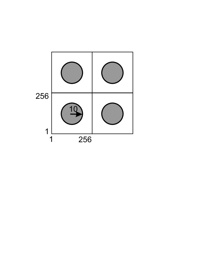
Figure 1: Pictorial view of the initial condition taken in a two-dimensional cell of 256² points with periodic boundary conditions. The outward velocity (or the density) takes distinct values inside and outside the circle of radius 10, while the remaining variables are taken homogeneous throughout the cell.

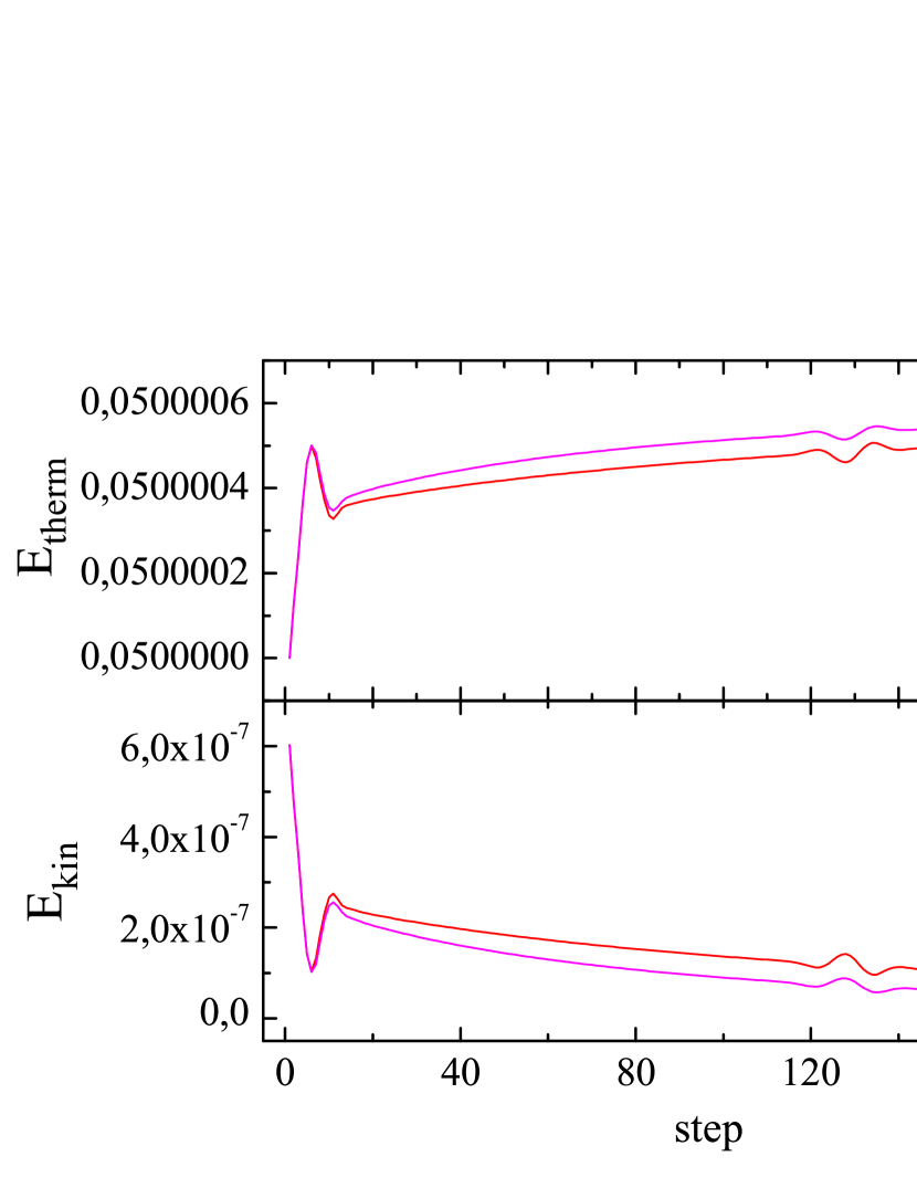
Figure 2: The thermal and the kinetic energies for the Maxwell-Boltzmann distribution, with the circle of radial velocity as initial condition, are shown here for the first 200 time steps, using both the d2q17 and d2q37 lattices. For time step 118 the travelling front wave hits the side of the unit cell.

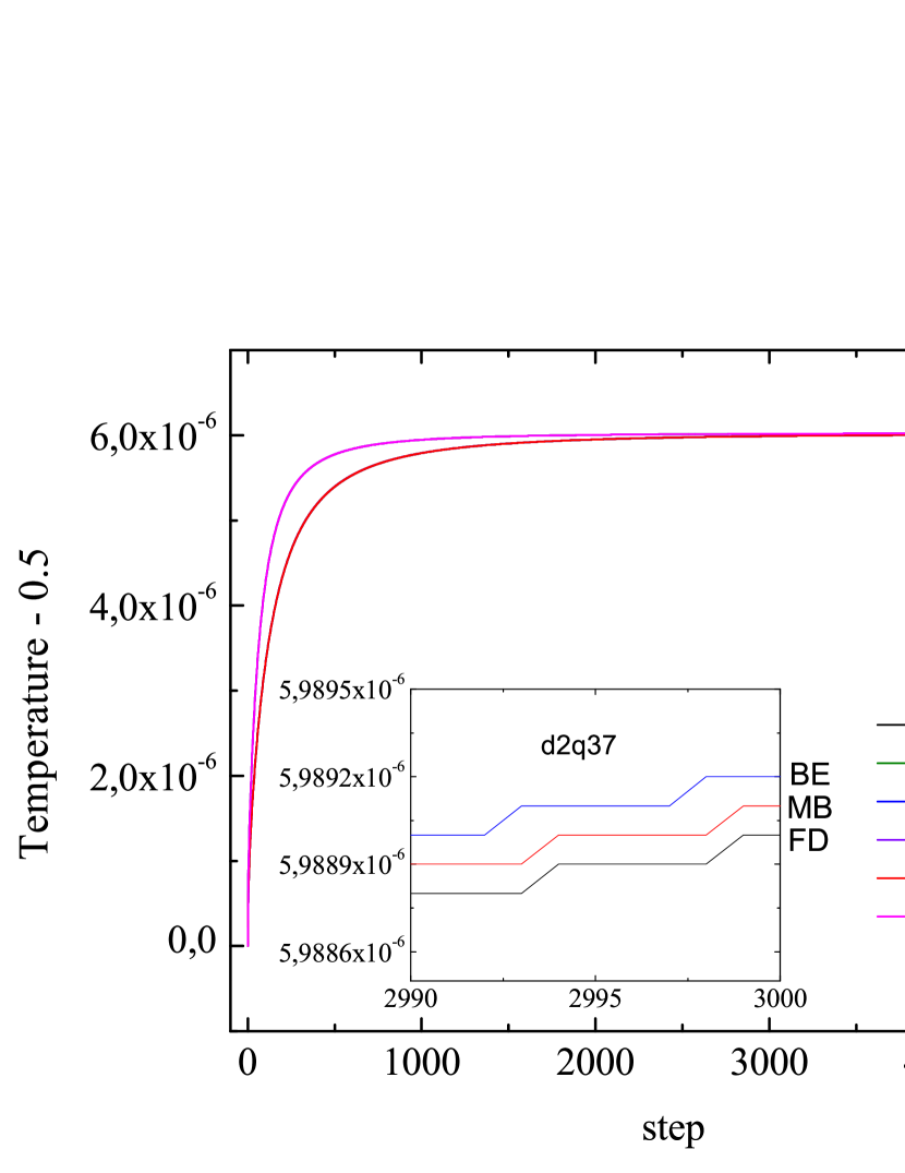
Figure 3: The deviation of the temperature from its initial value is shown here for the first 5000 time steps using the circle of velocity as initial condition. The the splitting among the FD, MB and BE distribution curves is very small in comparison to the d2q17 and d2q37 lattice splitting and for this reason not observable. The inset shows for a particular time step window the splitting of the temperature deviation among the three distributions for the d2q37 lattice.

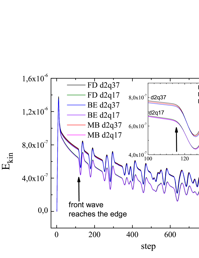
Figure 4: The Kinetic energy of the FD, MB and BE distributions using the d2q17 and d2q37 lattices is shown here for the first 1000 time steps. The initial condition used is of the circle of density. The inset shows in a particular time step window the splitting of the kinetic energy among the three distributions for both d2q17 and d2q37 lattices.

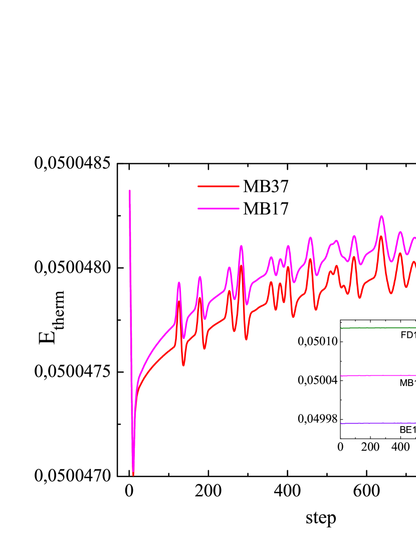
Figure 5: The thermal energy of the MB distribution using the d2q17 and d2q37 lattices is shown here for the first 1000 time steps. The initial condition used is that of the circle of density. The inset shows in a particular time step window the splitting of the kinetic energy among the three distributions for the d2q17 lattice.

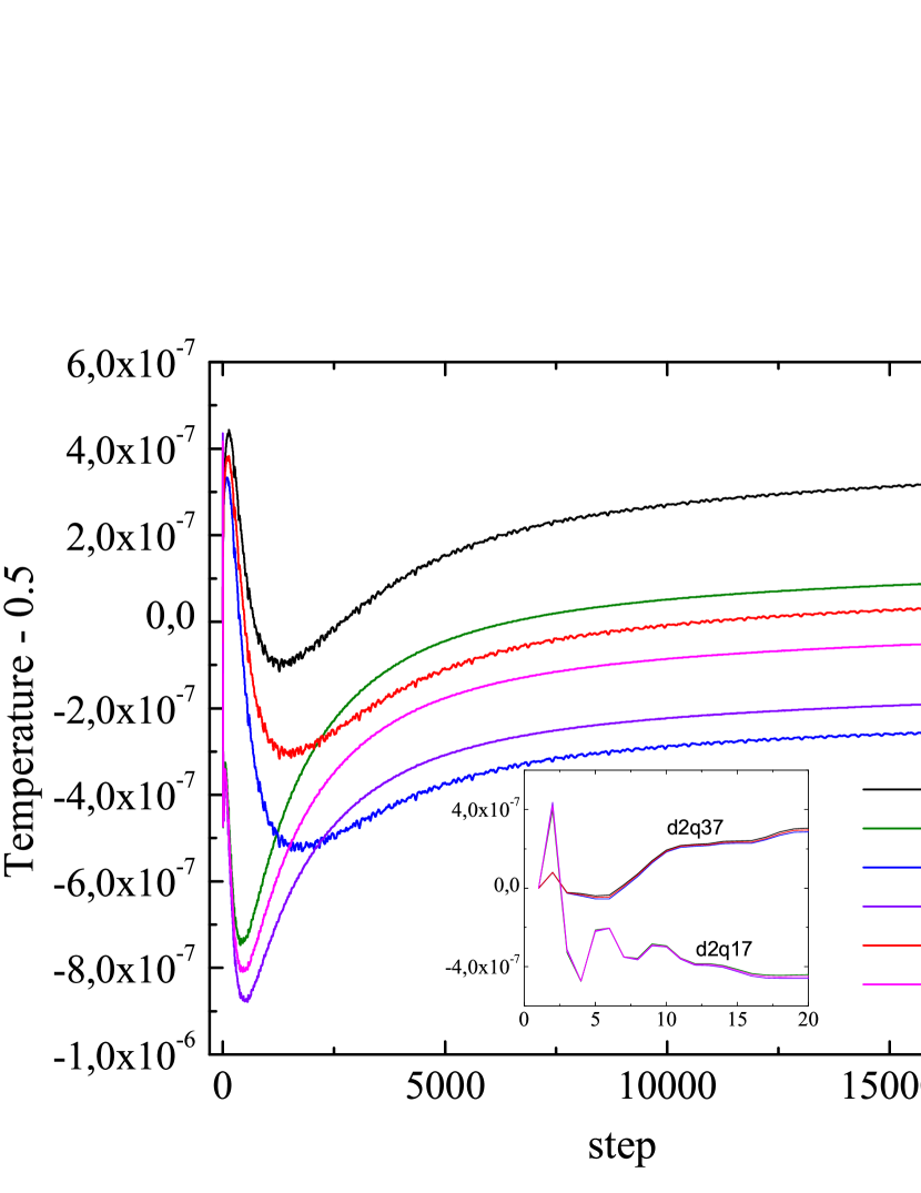
Figure 6: The temperature deviation from its initial value is shown here for the case of a circle of density as initial condition for the first 20000 time steps. The curves for the three distributions and the two lattices are clearly seen here. The inset shows the first 20 time steps.

VIII Numerical results

In this section we use the LBM based on the present $N=4$ order theory to numerically solve the dilute quantum fluid. We find that the energy is indeed conserved in $D=2$ under periodic boundary conditions and some initial conditions that trigger a time evolution where motion and heat occur simultaneously. The initial conditions are associated to a circle of radius $R$ located at the center of the cell, where one of the variables, among the temperature $\theta$, velocity $\boldsymbol{u}$, and the density $\rho$, assumes a special value, whereas the other two are taken constant throughout the cell. A pictorial view of such initial conditions is shown in Fig. 1. We work with a grid of $A_{cell}=256^{2}$ points, and in these units $R=10$. We take for the time step of Eq.(I) $\tau/\Delta t=0.58$. We use in this section the concept of a real temperature $T$ connected to the reduced one by $T\equiv c_{s}^{2}\theta$, where $c_{s}$ is a distinct numerical parameter for each of the lattices d2q17 and d2q37, This parameter makes equal to one the smallest non-zero microscopic velocity along the axis PhysRevE.77.026707 . In dimensionless units $c_{s}$ plays the role of the speed $c_{r}$, defined by Eq.(37). The time evolution of the system is a multiple of the computer steps performed in our numerical procedure. Since our goal is to verify that the total energy remains constant in the cell at any time step, we define the following sums over all cell points, which are the average values of the kinetic and the thermal energies in the cell.

$$E_{kin}\equiv\frac{1}{A_{cell}}\sum_{cell}\frac{1}{2}\rho\boldsymbol{u}^{2}$$ (151)

$$E_{therm}\equiv\frac{1}{A_{cell}}\sum_{cell}\frac{D}{2}\rho\bar{\theta},\,\mbox{and}$$ (152)

$$E_{total}\equiv E_{kin}+E_{therm},$$ (153)

In our numerical study we assume identical initial conditions for the BE, FD and MB cases, which means that they start with the same density, temperature and velocity. Thus the initial kinetic energy of Eq.(151) is the same for the three cases, but not the thermal energy of Eq.(152) since the initial pseudo temperature is not the same for the three cases, according to Eq.(150), being greater for fermions and smaller for bosons, as compared to the classical case.

To perform numerical calculations we must employ a concrete realization of the weights and microscopic velocities that satisfy the algebra of Eqs.(81) to (87). This assures that the Gauss-Hermite quadrature is being correctly performed. We choose the so-called d2q17 FLM:409537 and d2q37 PhysRevE.77.026707 microscopic velocity lattices. It is important to make a few considerations about these lattices regarding their ability to give the expected answers. This ability relies on the order of the maximum power of the microscopic velocity polynomial contained in the equilibrium distribution function and also the calculated moments. The equilibrium distribution function has maximum order ${f}^{(0)}_{\alpha}\sim\xi_{\alpha}^{N}$, for $N=3$ and $N=4$, as seen from Eq.(VI) and Eq.(IV), respectively. For computer purposes the highest moment that must be calculated is the energy, which is of order $\xi_{\alpha}^{2}$. Thus the chosen microscopic velocity lattice must correctly account for the sums of the kind Eqs.(81) to (87), which means $\xi_{\alpha}^{5}$ for $N=3$ and $\xi_{\alpha}^{6}$ for $N=4$. According to Ref. FLM:409537, these calculations can be correctly done in the d2q9 and d2q17 algebras for $N=3$ and $N=4$, respectively. Thus we conclude that d2q17 and d2q37 can be used for the numerical treatment of the present $N=4$ order LBM. Nevertheless to apply the Chapman-Enskog analysis and derive the equation for energy, one must compute the moment $\phi^{jk}\sim\xi_{\alpha}^{4}{f}^{(0)}_{\alpha}$. Hence in this case the microscopic velocity lattice must correctly account for sums beyond Eqs.(81) to (87), which means of the order $\xi_{\alpha}^{7}$ for $N=3$ and $\xi_{\alpha}^{8}$ for $N=4$. Thus for this purpose the d2q17 lattice is limited to $N=3$ FLM:409537 and cannot be used $N=4$. For such purpose $N=4$ demands a higher order lattice, such as d2q37 PhysRevE.77.026707 .

VIII.1 Velocity initial conditions

Under this initial condition $\boldsymbol{u}$ is non-zero inside a circle of radius $R$, where the outward component is equal to 0.02 in reduced units, being zero outside the circle. Thus at the beginning radial motion is set for a dilute quantum fluid of constant density, $\rho=0.1$, and temperature, $T=0.5$, in the unit cell. This initial motion immediately generates friction and subsequent heating that raises the temperature. Fig. 2 shows the time step evolution of $E_{kin}$ and $E_{therm}$ and the most important aspect found in these two plots is that their sum is a constant which is $E_{total}$, as given by Eq.(153). $E_{kin}$ follows the trend of decrease in time, and eventually must vanish, while $E_{therm}$ increases and tends to stabilize, though such behaviours are just suggested in the first 200 steps of Fig. 2. This figure only intends to display the evolution immediately after the initial condition. To reach a nearly steady state of zero velocity and stable temperature simulations up to 20.000 steps must be carried. The two employed lattices, namely d2q17 and d2q37, give the same qualitative results for the time evolution of the system, but their numerical difference hinders the splitting among the BE, FD and MB curves for each lattice as they fall very close to each other. Notice the non-zero initial value of $E_{kin}$, due to the initial velocity condition. After a few steps $E_{kin}$ drops to a local minimum, which is a local maximum for $E_{therm}$, meaning that friction caused by motion raises the temperature but in such a way that $E_{total}$ is conserved. After 118 steps the front wave raised by the initial condition reaches the side of the unit cell. Notice that this number coincides with the number of grid points between the circle and the unit cell side, namely, (256-20)/2. In the numerical algorithm the speed of propagation is one, thus the number of steps required for the signal reach the border is the number of grid points itself. Indeed Fig. 2 shows a hilly behaviour starting nearly at 120 steps, a consequence of the interference of incoming waves from the neighbour cells. Fig. 3 shows the evolution of the temperature deviation from its initial value of $T=0.5$. After 5000 steps the d2q17 and the d2q37 converge basically to the same final temperature which is just $6.0\;10^{-6}$ above the initial one. Interestingly there is also oscillatory behaviour in the deviated temperature though much less perceptible than in Fig. 2. The inset of Fig. 3 shows the splitting between the BE, FD and MB cases in a particular time step window. Indeed one observes that this splitting between the three statistics is of order $10^{-9}$ whereas the differences between d2q17 and d2q37 is of order $10^{-6}$.

VIII.2 Density initial conditions

Under this initial condition the density is $\rho=0.12$ inside and $\rho=0.1$ outside the circle of radius $R$. The initial temperature is $T=0.5$ and the macroscopic velocity $\boldsymbol{u}$ is zero everywhere. Though there is no initial motion, the non homogeneous density distribution sets a pressure front. The higher density at the center means higher pressure that forces motion outward the circle, and so, generates friction, heating and raise of the temperature in the cell. The first 1000 steps of $E_{kin}$ are shown in Fig. 2. Notice that it starts from zero and the oscillatory behavior set by the entrance of wave fronts from neighbor cells is well described by the d2q17 and d2q37 lattices since their numerical differences are in the range of $10^{-7}$. In this case too the difference among the three distributions is hidden by the lattice difference, shown in the inset for a chosen window of time steps for both lattices. The trend towards kinetic energy decay is seen in this figure though the convergence towards a steady state is only suggested by this figure. To really see it a larger window must be taken. The time step evolution of $E_{therm}$ is shown in Fig.(5). $E_{therm}$ experiments a sudden drop to allow for the increase of $E_{kin}$ as the system starts motion due to pressure unbalance. As in the previously case, $E_{total}$ is absolutely conserved to machine precision, in our case tested to order $10^{-10}$. The inset of this plot shows the splitting of the three distributions within the first 1000 steps. Notice that such values are distinct because we chose the same initial $\theta$ for the three distributions, which means different $\bar{\theta}$ in the three cases. Finally we address the evolution of the temperature deviation from its initial value $T=0.5$ in Fig.(6) within the full time step window studied, namely 20000 steps. The very first 20 steps, shown in the inset, indicate that the initial temperature is the same in all cases. However the final ones are different. The d2q17 reaches a final temperature deviation at a value slightly lower that the d2q37 case by an order of magnitude of $10^{-7}$. The final deviation is higher for the FD distribution and lower for the BE. We notice during evolution a drop to a minimum of temperature required to accommodate the kinetic expansion caused by the pressure unbalance in an energy conserving scenario.

IX Conclusion

We have conclusively shown that the Hermite polynomial expansion of the equilibrium distribution functions must be carried to fourth order for quantum fluids. Only in this order it is possible to obtain meaningful macroscopic hydrodynamical equations that lead to the correct viscosity and thermal coefficients. We have also demonstrated the feasibility of the fourth order lattice Boltzmann method scheme by showing that it numerically describes motion and heating in an energy conserving way.

Appendix A Hermite polynomials

The lowest order Hermite polynomials are easily derived from Eq.(51):

$$H(\boldsymbol{\xi})=1$$ (154)

$$H^{i}(\boldsymbol{\xi})=\xi^{i}$$ (155)

$$H^{ij}(\boldsymbol{\xi})=\xi^{i}\xi^{j}-\delta^{ij}$$ (156)

$$H^{ijk}(\boldsymbol{\xi})=\xi^{i}\xi^{j}\xi^{k}-(\xi^{i}\delta^{jk}+\xi^{j}\delta^{ik}+\xi^{k}\delta^{ij})$$ (157)

$$H^{ijkl}(\boldsymbol{\xi})=\xi^{i}\xi^{j}\xi^{k}\xi^{l}-(\xi^{i}\xi^{j}\delta^{kl}+\xi^{i}\xi^{k}\delta^{jl}+\xi^{i}\xi^{l}\delta^{jk}+$$

$$+\xi^{j}\xi^{k}\delta^{il}+\xi^{j}\xi^{l}\delta^{ik}+\xi^{k}\xi^{l}\delta^{ij})+\delta^{ijkl}.$$ (158)

The following integrals over the gaussian function of Eq.(52) are a consequence of the orthonormality of the Hermite polynomials:

$$\int d^{D}\boldsymbol{\xi}\,\omega(\boldsymbol{\xi})=1$$ (159)

$$\int d^{D}\boldsymbol{\xi}\,\omega(\boldsymbol{\xi})\xi^{i}=0$$ (160)

$$\int d^{D}\boldsymbol{\xi}\,\omega(\boldsymbol{\xi})\xi^{i}\xi^{j}=\delta^{ij}$$ (161)

$$\int d^{D}\boldsymbol{\xi}\,\omega(\boldsymbol{\xi})\xi^{i}\xi^{j}\xi^{k}=0$$ (162)

$$\int d^{D}\boldsymbol{\xi}\,\omega(\boldsymbol{\xi})\xi^{i}\xi^{j}\xi^{k}\xi^{l}=\delta^{ijkl}$$ (163)

$$\int d^{D}\boldsymbol{\xi}\,\omega(\boldsymbol{\xi})\xi^{i}\xi^{j}\xi^{k}\xi^{l}\xi^{m}=0$$ (164)

$$\int d^{D}\boldsymbol{\xi}\,\omega(\boldsymbol{\xi})\xi^{i}\xi^{j}\xi^{k}\xi^{l}\xi^{m}\xi^{n}=\delta^{ijklmn}.$$ (165)

The $\delta^{\cdots}$ tensors are constructed recursively from the Kronecker´s symbol: $\delta^{ij}=1$ for $i=j$ and 0 for $i\neq j$. In case of four indices,

$$\delta^{ijkl}\equiv\delta^{ij}\delta^{kl}+\delta^{ik}\delta^{jl}+\delta^{il}\delta^{kj}.$$ (166)

The sixth order tensor is,

$$\delta^{ijklmn}\equiv\delta^{ij}\delta^{klmn}+\delta^{ik}\delta^{jlmn}+$$

$$+\delta^{il}\delta^{kjmn}+\delta^{im}\delta^{jkln}+\delta^{in}\delta^{jklm}.$$ (167)

The eight order is,

$$\delta^{ijklmnpq}\equiv\delta^{ij}\delta^{klmnpq}+\delta^{ik}\delta^{jlmnpq}+\delta^{il}\delta^{jkmnpq}+$$

$$+\delta^{im}\delta^{jklnpq}+\delta^{in}\delta^{jklmpq}+\delta^{ip}\delta^{jklmnq}+\delta^{iq}\delta^{jklmnp},$$

and so forth.

To illustrate that Eqs.(160-165) are a consequence of Eq.(53) let us consider two examples. The orthogonality of the first two Hermite polynomials is,

$$\int d^{D}\boldsymbol{\xi}\,\omega(\xi)H(\boldsymbol{\xi})H^{i}(\boldsymbol{\xi})=\int d^{D}\boldsymbol{\xi}\,\omega(\xi)\xi^{i}=0,$$ (169)

which yields Eq.(160). Integration over two first order Hermite polynomials gives,

$$\int d^{D}\boldsymbol{\xi}\,\omega(\xi)H^{i}(\boldsymbol{\xi})H^{j}(\boldsymbol{\xi})=\int d^{D}\boldsymbol{\xi}\,\omega(\xi)\xi^{i}\xi^{j}=\delta^{ij},$$ (170)

which is Eq.(161). Integration over the first and the second order Hermite polynomials gives that,

$$\int d^{D}\boldsymbol{\xi}\,\omega(\xi)H^{i}(\boldsymbol{\xi})H^{jk}(\boldsymbol{\xi})=$$ (171)

$$=\int d^{D}\boldsymbol{\xi}\,\omega(\xi)\xi^{i}\left(\xi^{j}\xi^{k}-\delta^{jk}\right)=0.$$ (172)

From Eq.(169) one obtains Eq.(162). As a last example we consider the integration over two second order Hermite polynomials:

$$\int d^{D}\boldsymbol{\xi}\,\omega(\boldsymbol{\xi})H^{ij}(\boldsymbol{\xi})H^{kl}(\boldsymbol{\xi})=$$

$$=\int d^{D}\boldsymbol{\xi}\,\omega(\boldsymbol{\xi})[\xi^{i}\xi^{j}-\delta^{ij}][\xi^{k}\xi^{l}-\delta^{kl}]=$$

$$=\int d^{D}\boldsymbol{\xi}\,\omega(\boldsymbol{\xi})\xi^{i}\xi^{j}\xi^{k}\xi^{l}-\delta^{ij}\int d^{D}\boldsymbol{\xi}\,\omega(\boldsymbol{\xi})\xi^{k}\xi^{l}-$$

$$-\delta^{kl}\int d^{D}\boldsymbol{\xi}\,\omega(\boldsymbol{\xi})\xi^{i}\xi^{j}+\delta^{ij}\delta^{kl}\int d^{D}\boldsymbol{\xi}\,\omega(\boldsymbol{\xi})=$$

$$=\delta^{ik}\delta^{jl}+\delta^{il}\delta^{kj}.$$

The orthogonality relations, given by Eqs.(160)-(165) are the key ingredients to obtain the moments of Eqs.(188), (189) and (190).

It is worth to investigate the properties of the Hermite polynomials in case the argument is a difference $\xi-u$. Using (154), (155), (156), (157) we find the following relations:

$$H^{i}(\boldsymbol{\xi})=H^{i}(\boldsymbol{\xi-u})+u^{i}H$$ (173)

$$H^{ij}(\boldsymbol{\xi})=H^{ij}(\boldsymbol{\xi-u})+u^{i}H^{j}(\boldsymbol{\xi-u})+$$

$$+u^{j}H^{i}(\boldsymbol{\xi-u})+u^{i}u^{j}H$$ (174)

$$H^{ijk}(\boldsymbol{\xi})=H^{ijk}(\boldsymbol{\xi-u})+u^{i}H^{jk}(\boldsymbol{\xi-u})+$$

$$+u^{j}H^{ik}(\boldsymbol{\xi-u})+u^{k}H^{ij}(\boldsymbol{\xi-u})+u^{i}u^{j}H^{k}(\boldsymbol{\xi-u})+$$

$$+u^{i}u^{k}H^{j}(\boldsymbol{\xi-u})+u^{j}u^{k}H^{i}(\boldsymbol{\xi-u})+u^{i}u^{j}u^{k}H$$ (175)

$$H^{ijkl}(\boldsymbol{\xi})=H^{ijkl}(\boldsymbol{\xi-u})+u^{i}H^{jkl}(\boldsymbol{\xi-u})+$$

$$+u^{j}H^{ikl}(\boldsymbol{\xi-u})+u^{k}H^{ijl}(\boldsymbol{\xi-u})+u^{l}H^{ijk}(\boldsymbol{\xi-u})+$$

$$+u^{i}u^{j}H^{kl}(\boldsymbol{\xi-u})+u^{i}u^{k}H^{jl}(\boldsymbol{\xi-u})+u^{i}u^{l}H^{jk}(\boldsymbol{\xi-u})+$$

$$+u^{k}u^{l}H^{ij}(\boldsymbol{\xi-u})+u^{j}u^{l}H^{ik}(\boldsymbol{\xi-u})+u^{j}u^{k}H^{il}(\boldsymbol{\xi-u})+$$

$$+u^{i}u^{j}u^{k}H^{l}(\boldsymbol{\xi-u})+u^{i}u^{j}u^{l}H^{k}(\boldsymbol{\xi-u})+$$

$$+u^{j}u^{k}u^{l}H^{i}(\boldsymbol{\xi-u})+u^{i}u^{k}u^{l}H^{j}(\boldsymbol{\xi-u})+$$

$$+u^{i}u^{j}u^{k}u^{l}.$$ (176)

Using the above expressions it becomes straightforward to calculate the first four coefficients of the Hermite expansion.

Appendix B Taylor expansion of the Maxwell-Boltzmann distribution function

In this Appendix we consider the Maxwell-Boltzmann equilibrium distribution in reduced units,

$$f(\boldsymbol{\xi})\equiv\rho\left(\frac{1}{2\pi\theta}\right)^{\frac{D}{2}}e^{-\frac{(\boldsymbol{\xi}-\boldsymbol{u})^{2}}{2\theta}},$$ (177)

whose first three moments are obtained as below.

$$\rho(\boldsymbol{x}) = \int d^{D}\boldsymbol{\xi}f(\boldsymbol{\xi}),$$ (178)

$$\boldsymbol{u}(\boldsymbol{x}) = \frac{1}{\rho(\boldsymbol{x})}\int d^{D}\boldsymbol{\xi}\;\boldsymbol{\xi}f(\boldsymbol{\xi}),\,\mbox{and},$$ (179)

$$\frac{D}{2}\theta(\boldsymbol{x}) = \frac{1}{\rho(\boldsymbol{x})}\int d^{D}\boldsymbol{\xi}\;\frac{1}{2}\left[\boldsymbol{\xi}-\boldsymbol{u}(\boldsymbol{x})\right]^{2}f(\boldsymbol{\xi}).$$ (180)

We seek a Taylor expansion of the Maxwell-Boltzmann equilibrium distribution function such that the three above moment relations are retained for the expanded distribution function. The reference temperature and velocity are the parameters that set the Taylor expansion, although they are not present in the original distribution. This means that the limit that the macroscopic velocity and the temperature deviation are small in comparison to $c_{r}$ and $T_{r}$, respectively, is being considered. Therefore $\boldsymbol{u}(\boldsymbol{x})$ and $\theta(\boldsymbol{x})-1$ are small quantities, fact that justifies a series expansion in powers of these quantities. The present Taylor expansion makes evident the presence of a small parameter $\epsilon$ and we take the expansion until order $\epsilon^{2}$. The square of the macroscopic velocity and the temperature deviation must be considered of the same order: $|\boldsymbol{u}(\boldsymbol{x})|\sim\sqrt{\epsilon}$ and $\theta(\boldsymbol{x})-1\sim\epsilon$. A few remarks are worth of notice. The only scalars available are $\boldsymbol{\xi\cdot u}$ and $\boldsymbol{u}^{2}$. The microscopic velocity $\boldsymbol{\xi}$ has no $\epsilon$ order assigned to it being limited to small values by the gaussian decay. Therefore according to our expansion criterion the only terms to be kept are those proportional to 1, $\boldsymbol{\xi\cdot u}$, $\boldsymbol{u}^{2}$, $(\boldsymbol{\xi\cdot u})^{2}$, $\boldsymbol{u}^{3}$, $(\boldsymbol{\xi\cdot u})^{2}\boldsymbol{u}$, $(\boldsymbol{\xi\cdot u})\boldsymbol{u}^{2}$, $(\boldsymbol{\xi\cdot u})^{3}$, $\boldsymbol{u}^{4}$, $(\boldsymbol{\xi\cdot u})^{2}\boldsymbol{u}^{2}$, $(\boldsymbol{\xi\cdot u})^{4}$, $(\theta-1)$, $(\theta-1)\boldsymbol{\xi\cdot u}$, $(\theta-1)\boldsymbol{u}^{2}$, $(\theta-1)(\boldsymbol{\xi\cdot u})^{2}$, and $(\theta-1)^{2}$. Firstly consider small deviations of $T_{r}$, namely, $\theta=1+(\theta-1)$ up to order $\epsilon^{2}$ in the denominator of Eq.(177):

$$\frac{1}{\theta^{\frac{D}{2}}}=\frac{1}{[1+(\theta-1)]^{\frac{D}{2}}}=$$

$$=1-\frac{D}{2}(\theta-1)+\frac{D}{4}\frac{D+2}{2}(\theta-1)^{2}+O(\epsilon^{3}).$$ (181)

The exponential also has a $\theta$ dependent denominator that must be expanded resulting in three different terms, which must be treated separately according to $\epsilon$.

$$\exp\left(-\frac{(\boldsymbol{\xi}-\boldsymbol{u})^{2}}{2\theta}\right)=$$ (182)

$$= \exp\left\{-\frac{(\boldsymbol{\xi}-\boldsymbol{u})^{2}}{2}\left[1-(\theta-1)+(\theta-1)^{2}+O(\epsilon^{3})\right]\right\}=$$

$$= \exp\left[-\left(\frac{\boldsymbol{\xi}^{2}}{2}-\boldsymbol{\xi\cdot u}+\frac{\boldsymbol{u}^{2}}{2}\right)\right]\cdot$$

$$\cdot\exp\left[\left(\frac{\boldsymbol{\xi}^{2}}{2}-\boldsymbol{\xi\cdot u}+\frac{\boldsymbol{u}^{2}}{2}\right)(\theta-1)\right]\cdot$$

$$\cdot\exp\left[-\left(\frac{\boldsymbol{\xi}^{2}}{2}-\boldsymbol{\xi\cdot u}+\frac{\boldsymbol{u}^{2}}{2}\right)(\theta-1)^{2}\right]\ldots$$

In the first exponential we factorize the gaussian function (Eq.(52)), $\exp\left(-\boldsymbol{\xi}^{2}/2\right)$, because of its zeroth $\epsilon$ order. Next we select for the three exponentials only those terms of order equal or lower than $\epsilon^{2}$. The first exponential becomes

$$\exp\left[-\left(\frac{\boldsymbol{\xi}^{2}}{2}-\boldsymbol{\xi\cdot u}+\frac{\boldsymbol{u}^{2}}{2}\right)\right]=\exp{\left(-\frac{\boldsymbol{\xi}^{2}}{2}\right)}\cdot$$

$$[1+\boldsymbol{\xi\cdot u}-\frac{\boldsymbol{u}^{2}}{2}+\frac{1}{2}(\boldsymbol{\xi\cdot u})^{2}-\frac{1}{2}(\boldsymbol{\xi\cdot u})\boldsymbol{u}^{2}+$$ (183)

$$\frac{\boldsymbol{u}^{4}}{8}+\frac{1}{6}(\boldsymbol{\xi\cdot u})^{3}-\frac{1}{4}(\boldsymbol{\xi\cdot u})^{2}\boldsymbol{u}^{2}+\frac{1}{24}(\boldsymbol{\xi\cdot u})^{4}+O(\epsilon^{5/2})].$$

The second one,

$$\exp\left[-\left(\frac{\boldsymbol{\xi}^{2}}{2}-\boldsymbol{\xi\cdot u}+\frac{\boldsymbol{u}^{2}}{2}\right)(\theta-1)\right]=1+$$ (184)

$$+\left(\frac{\boldsymbol{\xi}^{2}}{2}-\boldsymbol{\xi\cdot u}+\frac{\boldsymbol{u}^{2}}{2}\right)(\theta-1)+\frac{\boldsymbol{\xi}^{4}}{8}(\theta-1)^{2}+O(\epsilon^{5/2}),$$

and the third,

$$\exp\left[-\left(\frac{\boldsymbol{\xi}^{2}}{2}-\boldsymbol{\xi\cdot u}+\frac{\boldsymbol{u}^{2}}{2}\right)(\theta-1)^{2}\right]=$$

$$= 1-\frac{\boldsymbol{\xi}^{2}}{2}(\theta-1)^{2}+O(\epsilon^{5/2}).$$

The product of Eqs.(181) and (182), together with the expansions of Eq.(183), (184), (B), gives that

$$f=\rho\omega(\boldsymbol{\xi})\left[1-\frac{D}{2}(\theta-1)+\frac{D}{4}\frac{D+2}{2}(\theta-1)^{2}-O(\epsilon^{3})\right]\cdot$$

$$\cdot\big{[}1+\boldsymbol{\xi\cdot u}-\frac{\boldsymbol{u}^{2}}{2}+\frac{1}{2}(\boldsymbol{\xi\cdot u})^{2}-\frac{1}{2}(\boldsymbol{\xi\cdot u})\boldsymbol{u}^{2}+\frac{\boldsymbol{u}^{4}}{8}+$$

$$+\frac{1}{6}(\boldsymbol{\xi\cdot\vec{u}})^{3}-\frac{1}{4}(\boldsymbol{\xi\cdot u})^{2}\boldsymbol{u}^{2}+\frac{1}{24}(\boldsymbol{\xi\cdot u})^{4}-O(\epsilon^{5/2})\big{]}\cdot\big{[}1+$$

$$+\left(\frac{\boldsymbol{\xi}^{2}}{2}-\boldsymbol{\xi\cdot u}+\frac{\boldsymbol{u}^{2}}{2}\right)(\theta-1)+\frac{\boldsymbol{\xi}^{4}}{8}(\theta-1)^{2}+O(\epsilon^{5/2})\big{]}\cdot$$

$$\cdot\big{[}1-\frac{\boldsymbol{\xi}^{2}}{2}(\theta-1)^{2}+O(\epsilon^{5/2})\big{]}$$ (186)

where we have used the gaussian function of Eq.(52). Finally we expand Eq.(B) and hold terms up to order $\epsilon^{2}$, by multiplying the $\epsilon$ expansions of the three exponentials of the numerator with that of the denominator:

$$\frac{\bar{f}}{\rho\omega(\boldsymbol{\xi})}=1+\boldsymbol{\xi\cdot u}+\frac{1}{2}(\boldsymbol{\xi\cdot u})^{2}-\frac{u^{2}}{2}+\frac{1}{2}(\theta-1)(\boldsymbol{\xi}^{2}-D)+$$

$$+\frac{1}{6}(\boldsymbol{\xi\cdot u})^{3}-\frac{1}{2}\boldsymbol{u}^{2}(\boldsymbol{\xi\cdot u})+\frac{1}{2}(\theta-1)(\boldsymbol{\xi\cdot u})(\boldsymbol{\xi}^{2}-D-2)+$$

$$+\frac{1}{24}(\boldsymbol{\xi\cdot u})^{4}-\frac{1}{4}(\boldsymbol{\xi\cdot u})^{2}\boldsymbol{u}^{2}+\frac{1}{8}\boldsymbol{u}^{4}+$$

$$+\frac{1}{4}(\theta-1)\big{[}(\boldsymbol{\xi\cdot u})^{2}(\boldsymbol{\xi}^{2}-D-4)+\boldsymbol{u}^{2}(D+2-\boldsymbol{\xi}^{2})\big{]}+$$

$$+\frac{1}{8}(\theta-1)^{2}\big{[}\boldsymbol{\xi}^{4}-2(D+2)\boldsymbol{\xi}^{2}+D(D+2)\big{]}+O(\epsilon^{5/2})$$ (187)

We have obtained a Taylor expansion of the Maxwell Boltzmann equilibrium distribution function (Eq.(177)) in powers of $T(\boldsymbol{x})/T_{r}-1$ and $\boldsymbol{v(\boldsymbol{x})}/c_{r}$ up to the desired order of $\epsilon^{2}$. Remarkably, the three local parameters $\rho$, $\theta$, and $\boldsymbol{u}$, contained in $\bar{f}$, are also its first three moments. The above Taylor expansion also satisfies the same relations for the momentum flux tensor, $\int d^{D}\boldsymbol{\xi}\,\xi^{i}\xi^{j}\,\bar{f}(\boldsymbol{\xi})=\delta^{ij}\rho\theta D+\rho u^{i}u^{j}$, and for the energy flux tensor, $\int d^{D}\boldsymbol{\xi}\,\xi^{i}\boldsymbol{\xi}^{2}\,\bar{f}(\boldsymbol{\xi})=[\delta^{ij}\rho\theta(D+2)/2+\rho\boldsymbol{u}^{2}/2]u^{i}$.

$$\rho(\boldsymbol{x})=\int d^{D}\boldsymbol{\xi}\bar{f}(\boldsymbol{\xi},\rho,\theta,\boldsymbol{u}),$$ (188)

$$\boldsymbol{u}(\boldsymbol{x})=\frac{1}{\rho(\boldsymbol{x})}\int d^{D}\boldsymbol{\xi}\;\boldsymbol{\xi}\bar{f}(\boldsymbol{\xi},\rho,\theta,\boldsymbol{u}),$$ (189)

and,

$$\frac{D}{2}\theta(\boldsymbol{x})=\frac{1}{\rho(\boldsymbol{x})}\int d^{D}\boldsymbol{\xi}\;\frac{\left[\boldsymbol{\xi}-\boldsymbol{u}(\boldsymbol{x})\right]^{2}}{2}\bar{f}(\boldsymbol{\xi},\rho,\theta,\boldsymbol{u}).$$ (190)

Appendix C The position and time cross derivative terms of the momentum and energy conservation equations

In this Appendix we seek replacement of the $\frac{\partial}{\partial x^{j}}\frac{\partial}{\partial t}$ terms contained in Eqs. (124) and (135) by position derivatives. The key to this step is to consider that terms proportional to the square of the collision time $\tau$, namely, proportional to $[\tau(1-\Delta t/2\tau)]^{2}$, are neglected. Thus it consider the above equations in the limit $\tau\rightarrow 0$ and $\Delta t/\tau$ fixed. Setting $\tau=0$ in Eqs. (124) and (135) gives that,

$$\frac{\partial}{\partial t}\left(\rho u^{i}\right)+\frac{\partial}{\partial x^{j}}\left(\rho\bar{\theta}\delta^{ij}+\rho u^{i}u^{j}\right)=0,$$ (191)

$$\frac{\partial}{\partial t}\left(\frac{\rho}{2}\boldsymbol{u}^{2}+\frac{\rho}{2}D\bar{\theta}\right)+\frac{\partial}{\partial x^{j}}\left[\left(\frac{\rho}{2}\boldsymbol{u}^{2}+\frac{\rho}{2}\bar{\theta}(D+2)\right)u^{j}\right]=0.$$

(192)

C.1 The momentum conservation equation

Introducing the continuity equation (Eq.(2)) into Eq. (191) gives,

$$\rho\frac{\partial u^{i}}{\partial t}+\frac{\partial}{\partial x^{j}}\left(\rho\bar{\theta}\delta^{ij}\right)+\rho u^{j}\frac{\partial u^{i}}{\partial x^{j}}=0.$$ (193)

We develop some identities from Eqs.(2) and, (193).

$$\frac{\partial}{\partial t}(\rho\boldsymbol{u}^{2})=\boldsymbol{u}^{2}\frac{\partial\rho}{\partial t}+2\rho u^{j}\frac{\partial u^{j}}{\partial t}=$$

$$=-\boldsymbol{u}^{2}\frac{\partial}{\partial x^{j}}(\rho u^{j})-2u^{j}\frac{\partial}{\partial x^{i}}\left(\rho\bar{\theta}\delta^{ij}\right)-u^{j}\frac{\partial}{\partial x^{j}}(\rho\boldsymbol{u}^{2})=$$

$$=-\frac{\partial}{\partial x^{j}}(\rho\boldsymbol{u}^{2}u^{j})-2u^{j}\frac{\partial}{\partial x^{j}}\left(\rho\bar{\theta}\right).$$ (194)

Introducing Eq.(194) into Eq.(192) gives the identity,

$$\frac{\partial}{\partial t}\left(\rho\bar{\theta}D\right)-2u^{j}\frac{\partial}{\partial x^{j}}\left(\rho\bar{\theta}\right)+\frac{\partial}{\partial x^{j}}\left[\rho\bar{\theta}(D+2)u^{j}\right]=0,$$

that can be expressed as,

$$\frac{\partial}{\partial t}\left(\rho\bar{\theta}D\right)=-\frac{\partial}{\partial x^{j}}\left(\rho\bar{\theta}Du^{j}\right)-2\rho\bar{\theta}\frac{\partial u^{j}}{\partial x^{j}}.$$ (195)

Starting from,

$$\frac{\partial}{\partial t}(\rho u^{i}u^{j})=u^{i}u^{j}\frac{\partial\rho}{\partial t}+\rho u^{j}\frac{\partial u^{i}}{\partial t}+\rho u^{i}\frac{\partial u^{j}}{\partial t},$$ (196)

and using the continuity equation, Eq.(2), and Eq.(193), yields that,

$$\frac{\partial}{\partial t}(\rho u^{i}u^{j})=-u^{i}u^{j}\frac{\partial}{\partial x^{k}}(\rho u^{k})-u^{k}\frac{\partial}{\partial x^{k}}(u^{i}u^{j})\rho-$$

$$-u^{j}\frac{\partial}{\partial x^{i}}\left(\rho\bar{\theta}\right)-u^{i}\frac{\partial}{\partial x^{j}}\left(\rho\bar{\theta}\right)=$$

$$=-\frac{\partial}{\partial x^{k}}(\rho u^{i}u^{j}u^{k})-u^{j}\frac{\partial}{\partial x^{i}}\left(\rho\bar{\theta}\right)-u^{i}\frac{\partial}{\partial x^{j}}\left(\rho\bar{\theta}\right).$$ (197)

Thus the temporal evolution,

$$\frac{\partial}{\partial t}\left(\rho\bar{\theta}\delta^{ij}+\rho u^{i}u^{j}\right)=-\frac{\partial}{\partial x^{k}}\left(\rho\bar{\theta}u^{k}\right)\delta^{ij}-\frac{2}{D}\rho\bar{\theta}\frac{\partial u^{k}}{\partial x^{k}}\delta^{ij}-$$

$$-\frac{\partial}{\partial x^{k}}(\rho u^{i}u^{j}u^{k})-u^{j}\frac{\partial}{\partial x^{i}}\left(\rho\bar{\theta}\right)-u^{i}\frac{\partial}{\partial x^{j}}\left(\rho\bar{\theta}\right),$$

is to be fed into Eq.(122) to allow for the substitution of the position and time cross derivative term:

$$\frac{\partial}{\partial t}\left(\rho\bar{\theta}\delta^{ij}+\rho u^{i}u^{j}\right)=-\frac{\partial}{\partial x^{k}}\left[\rho u^{k}\left(\bar{\theta}\delta^{ij}+u^{i}u^{j}\right)\right]-$$

$$-\frac{2}{D}\rho\bar{\theta}\frac{\partial u^{k}}{\partial x^{k}}\delta^{ij}-u^{j}\frac{\partial}{\partial x^{i}}\left(\rho\bar{\theta}\right)-u^{i}\frac{\partial}{\partial x^{j}}\left(\rho\bar{\theta}\right).$$ (198)

Finally we are able to write the addition of two terms proportional to $\tau$ in Eq. (124) in terms of the derivative of the viscosity stress tensor (Eq.(18)) by means of Eq.(198).

$$\frac{\partial}{\partial x^{j}}\frac{\partial}{\partial x^{k}}\left[\rho(u^{k}\delta^{ij}+u^{j}\delta^{ik}+u^{i}\delta^{jk})\bar{\theta}+\rho u^{i}u^{j}u^{k}\right]+$$

$$+\frac{\partial}{\partial x^{j}}\frac{\partial}{\partial t}\left[\rho\left(\bar{\theta}\delta^{ij}+u^{i}u^{j}\right)\right]=$$

$$=\frac{\partial}{\partial x^{j}}\frac{\partial}{\partial x^{i}}\left(\rho u^{j}\bar{\theta}\right)+\frac{\partial}{\partial x^{j}}\frac{\partial}{\partial x^{j}}\left(\rho\bar{\theta}u^{i}\right)-\frac{\partial}{\partial x^{i}}\left(\frac{2}{D}\rho\bar{\theta}\frac{\partial u^{k}}{\partial x^{k}}\right)-$$

$$-\frac{\partial}{\partial x^{j}}\left[u^{j}\frac{\partial}{\partial x^{i}}\left(\rho\bar{\theta}\right)\right]-\frac{\partial}{\partial x^{j}}\left[u^{i}\frac{\partial}{\partial x^{j}}\left(\rho\bar{\theta}\right)\right]=$$

$$=\frac{\partial}{\partial x^{j}}\left(\rho\bar{\theta}\frac{\partial u^{j}}{\partial x^{i}}\right)+\frac{\partial}{\partial x^{j}}\left(\rho\bar{\theta}\frac{\partial u^{i}}{\partial x^{j}}\right)-\frac{\partial}{\partial x^{i}}\left(\frac{2}{D}\rho\bar{\theta}\frac{\partial u^{k}}{\partial x^{k}}\right)=$$

$$=\frac{\partial}{\partial x^{j}}\left[\rho\bar{\theta}\left(\frac{\partial u^{j}}{\partial x^{i}}+\frac{\partial u^{i}}{\partial x^{j}}-\frac{2}{D}\frac{\partial u^{k}}{\partial x^{k}}\delta^{ij}\right)\right].$$ (199)

Substituting this result in Eq.(124), we obtain the momentum conservation equation of Eq.(21).

C.2 The energy conservation equation

Some identities are obtained here, similarly to the momentum equation case. From Eqs.(193) and (195), it follows that,

$$\frac{\partial}{\partial t}\left[(D+2)\rho\bar{\theta}u^{j}\right]=(D+2)u^{j}\frac{\partial}{\partial t}\left(\rho\bar{\theta}\right)+(D+2)\rho\bar{\theta}\frac{\partial u^{j}}{\partial t}=$$

$$=-(D+2)\Bigg{[}\frac{\partial}{\partial x^{k}}\left(\rho\bar{\theta}u^{j}u^{k}\right)+\frac{2}{D}\rho\bar{\theta}\frac{\partial u^{k}}{\partial x^{k}}u^{j}+\bar{\theta}\frac{\partial}{\partial x^{j}}\left(\rho\bar{\theta}\right)\Bigg{]}.$$

Using the continuity equation (Eq.(2)) and Eq.(193), one obtains that,

$$\frac{\partial}{\partial t}(\rho u^{j}\boldsymbol{u}^{2})=\frac{\partial\rho}{\partial t}u^{j}\boldsymbol{u}^{2}+\rho\frac{\partial u^{j}}{\partial t}\boldsymbol{u}^{2}+2\rho u^{j}u^{k}\frac{\partial u^{k}}{\partial t}=$$

$$=-\frac{\partial}{\partial x^{k}}\left(\rho u^{k}u^{j}\boldsymbol{u}^{2}\right)-\frac{\partial}{\partial x^{j}}\left(\rho\bar{\theta}\right)\boldsymbol{u}^{2}-2u^{j}u^{k}\frac{\partial}{\partial x^{k}}\left(\rho\bar{\theta}\right).$$

Eqs.(C.2) and (C.2) allows to write the time dependent term of the position-time cross derivative in Eq. (135) as,

$$\frac{\partial}{\partial t}\left[\rho\boldsymbol{u}^{2}u^{j}+\rho\bar{\theta}(D+2)u^{j}\right]=$$

$$-\frac{\partial}{\partial x^{k}}\left[\rho u^{k}u^{j}\boldsymbol{u}^{2}+(D+2)\rho\bar{\theta}u^{j}u^{k}\right]-\frac{2}{D}(D+2)\rho\bar{\theta}\frac{\partial u^{k}}{\partial x^{k}}u^{j}-$$

$$-\left[(D+2)\bar{\theta}+\boldsymbol{u}^{2}\right]\frac{\partial}{\partial x^{j}}\left(\rho\bar{\theta}\right)-2u^{j}u^{k}\frac{\partial}{\partial x^{k}}\left(\rho\bar{\theta}\right).$$ (202)

Next we deal with the terms proportional to $\tau$ in the left side of Eq.(135) and apply Eq.(C.2) to it. For this define,

$$\tau\left[\cdots\right]\equiv\frac{1}{2}\frac{\partial}{\partial x^{j}}\frac{\partial}{\partial x^{k}}\left[\rho\boldsymbol{u}^{2}u^{j}u^{k}+\rho\bar{\theta}(D+4)u^{j}u^{k}+\right.$$

$$\left.+\rho\bar{\theta}\boldsymbol{u}^{2}\delta^{jk}+\rho\bar{\theta}^{2}(D+2)\delta^{jk}\right]+$$

$$+\frac{1}{2}\frac{\partial}{\partial x^{j}}\frac{\partial}{\partial t}\left[\rho u^{j}\boldsymbol{u}^{2}+\rho\bar{\theta}(D+2)u^{j}\right],$$ (203)

and substitute (C.2) into the above equation plus the cancelling of some terms, giving the final useful expression for the $\tau$ dependent terms of the left side of Eq.(135):

$$\tau\left[\cdots\right]=\frac{D+2}{2}\frac{\partial}{\partial x^{j}}\left(\rho{\bar{\theta}}\frac{\partial}{\partial x^{j}}{\bar{\theta}}\right)+$$

$$+\frac{\partial}{\partial x^{j}}\left[\rho\bar{\theta}u^{k}\left(\frac{\partial u^{k}}{\partial x^{j}}+\frac{\partial u^{j}}{\partial x^{k}}-\frac{2}{D}\frac{\partial u^{l}}{\partial x^{l}}\delta^{jk}\right)\right].$$ (204)

The above expression is introduced into Eq.(135), added to the definitions of the dynamic viscosity (Eq.(19)), the viscosity stress tensor (Eq.(18)) and the thermal conductivity (Eq.(20)).

Appendix D Useful Relations

$$\sum_{\alpha}\xi^{i}_{\alpha}\xi^{j}_{\alpha}\xi_{\alpha}^{k}\xi^{k}_{\alpha}w_{\alpha}=(D+2)\delta^{ij}$$ (205)

$$\sum_{\alpha}\xi^{i}_{\alpha}\xi^{j}_{\alpha}(\boldsymbol{\xi_{\alpha}\cdot u})^{2}w_{\alpha}=\boldsymbol{u}^{2}\delta^{ij}+2u^{i}u^{j}$$ (206)

$$\sum_{\alpha}\xi^{i}_{\alpha}\xi_{\alpha}^{j}(\boldsymbol{\xi_{\alpha}\cdot u})^{4}w_{\alpha}=3\boldsymbol{u}^{4}\delta^{ij}+12\boldsymbol{u}^{2}u^{i}u^{j}$$ (207)

$$\sum_{\alpha}\xi_{\alpha}^{i}\xi_{\alpha}^{j}(\boldsymbol{\xi_{\alpha}\cdot u})^{2}\boldsymbol{\xi_{\alpha}}^{2}w_{\alpha}=u^{i}u^{j}(2D+8)+\delta^{ij}(D+4)\boldsymbol{u}^{2}$$ (208)

$$\sum_{\alpha}\xi_{\alpha}^{i}\xi_{\alpha}^{j}\boldsymbol{\xi_{\alpha}}^{4}w_{\alpha}=\delta^{ij}(D^{2}+6D+8)$$ (209)

$$\sum_{\alpha}\xi_{\alpha}^{i}\xi_{\alpha}^{j}\xi_{\alpha}^{k}(\boldsymbol{\xi_{\alpha}\cdot u})w_{\alpha}=u^{k}\delta^{ij}+u^{j}\delta^{ik}+u^{i}\delta^{jk}$$ (210)

$$\sum_{\alpha}\xi_{\alpha}^{i}\xi_{\alpha}^{j}\xi^{k}_{\alpha}(\boldsymbol{\xi_{\alpha}\cdot u})^{3}w_{\alpha}=3(u^{k}\delta^{ij}+u^{j}\delta^{ik}+u^{i}\delta^{jk})\boldsymbol{u}^{2}+6u^{i}u^{j}u^{k}$$ (211)

$$\sum_{\alpha}\xi_{\alpha}^{i}\xi_{\alpha}^{j}\xi_{\alpha}^{k}(\boldsymbol{\xi_{\alpha}\cdot u})\boldsymbol{\xi_{\alpha}}^{2}w_{\alpha}=(D+4)(u^{k}\delta^{ij}+u^{j}\delta^{ik}+u^{i}\delta^{jk})$$ (212)

$$\sum_{\alpha}\boldsymbol{\xi_{\alpha}}^{2}w_{\alpha}=D$$ (213)

$$\sum_{\alpha}\boldsymbol{\xi_{\alpha}}^{2}(\boldsymbol{\xi_{\alpha}\cdot u})^{2}w_{\alpha}=(D+2)\boldsymbol{u}^{2}$$ (214)

$$\sum_{\alpha}\boldsymbol{\xi_{\alpha}}^{2}(\boldsymbol{\xi_{\alpha}\cdot u})^{4}w_{\alpha}=3(D+4)\boldsymbol{u}^{4}$$ (215)

$$\sum_{\alpha}\boldsymbol{\xi_{\alpha}}^{4}w_{\alpha}=D(D+2)$$ (216)

$$\sum_{\alpha}\boldsymbol{\xi_{\alpha}}^{4}(\boldsymbol{\xi_{\alpha}\cdot u})^{2}w_{\alpha}=(D+2)(D+4)\boldsymbol{u}^{2}$$ (217)

$$\sum_{\alpha}\boldsymbol{\xi_{\alpha}}^{6}w_{\alpha}=D^{3}+6D^{2}+8D$$ (218)

$$\sum_{\alpha}\boldsymbol{\xi_{\alpha}}^{2}\xi_{\alpha}^{i}(\boldsymbol{\xi_{\alpha}\cdot u})w_{\alpha}=(D+2)u^{j}$$ (219)

$$\sum_{\alpha}\boldsymbol{\xi_{\alpha}}^{2}\xi_{\alpha}^{j}(\boldsymbol{\xi_{\alpha}\cdot u})^{3}w_{\alpha}=3(D+4)u^{j}\boldsymbol{u}^{2}$$ (220)

$$\sum_{\alpha}\boldsymbol{\xi_{\alpha}}^{4}\xi_{\alpha}^{j}(\boldsymbol{\xi_{\alpha}\cdot u})w_{\alpha}=(D+4)(D+2)u^{j}$$ (221)

$$\sum_{\alpha}\boldsymbol{\xi_{\alpha}}^{2}\xi_{\alpha}^{j}\xi_{\alpha}^{k}(\boldsymbol{\xi_{\alpha}\cdot u})^{4}w_{\alpha}=3(D+6)(\boldsymbol{u}^{4}\delta^{jk}+4u^{j}u^{k}\boldsymbol{u}^{2})$$ (222)

$$\sum_{\alpha}\boldsymbol{\xi_{\alpha}}^{4}\xi_{\alpha}^{j}\xi_{\alpha}^{k}(\boldsymbol{\xi_{\alpha}\cdot u})^{2}w_{\alpha}=(D+4)(D+6)(\boldsymbol{u}^{2}\delta^{jk}+2u^{j}u^{k})$$ (223)

$$\sum_{\alpha}\boldsymbol{\xi_{\alpha}}^{6}\xi_{\alpha}^{j}\xi_{\alpha}^{k}w_{\alpha}=(D+2)(D+4)(D+6)\delta^{jk}$$ (224)

References

• (1) Yu-Hsin Shi and J.Y. Yang. A gas-kinetic {BGK} scheme for semiclassical boltzmann hydrodynamic transport. Journal of Computational Physics, 227(22):9389 – 9407, 2008.
• (2) Jaw-Yen Yang and Li-Hsin Hung. Lattice uehling-uhlenbeck boltzmann-bhatnagar-gross-krook hydrodynamics of quantum gases. Phys. Rev. E, 79:056708, May 2009.
• (3) Gilberto Medeiros Kremer. An Introduction to the Boltzmann Equation and Transport Processes in Gases. Springer-Verlag Berlin Heidelberg, 2010.
• (4) E. A. Uehling and G. E. Uhlenbeck. Transport phenomena in einstein-bose and fermi-dirac gases. i. Phys. Rev., 43:552–561, Apr 1933.
• (5) T. Nikuni and A. Griffin. Hydrodynamic damping in trapped bose gases. Journal of Low Temperature Physics, 111:793–814, 1998.
• (6) G. M. Kremer and C. H. Lepienski. On the kinetic theory of metal electrons. Journal of Non-Equilibrium Thermodynamics
• (7) Enrico Vogt, Michael Feld, Bernd Fröhlich, Daniel Pertot, Marco Koschorreck, and Michael Köhl. Scale invariance and viscosity of a two-dimensional fermi gas. Phys. Rev. Lett., 108:070404, Feb 2012.
• (8) P. L. Bhatnagar, E. P. Gross, and M. Krook. A model for collision processes in gases. i. small amplitude processes in charged and neutral one-component systems. Phys. Rev., 94:511–525, May 1954.
• (9) S. Succi. The Lattice Boltzmann Equation for Fluid Dynamics and Beyond. Clarendon Press, 2001.
• (10) M. Sukop and D. Thorne. Lattice Boltzmann Modeling. Springer-Verlag, 2006.
• (11) Dieter A. Wolf-Gladrow. Lattice-Gas Cellular Automata and Lattice Boltzmann Models - An Introduction. Springer, 2005.
• (12) A. A. Mohamad. Lattice Boltzmann Method. Springer-Verlag, 2011.
• (13) Xiaoyi He and Li-Shi Luo. A priori derivation of the lattice boltzmann equation. Phys. Rev. E, 55:R6333–R6336, Jun 1997.
• (14) L.D. Landau and E.M. Lifshitz. Fluid Mechanics. Robert Maxwell, M.C., 1986.
• (15) H. Grad. On the kinetic theory of rarefied gases. Commun. Pure Appl. Math., 2:331, 1949.
• (16) James F. Lutsko. Approximate solution of the enskog equation far from equilibrium. Phys. Rev. Lett., 78:243–246, Jan 1997.
• (17) Xiaowen Shan and Xiaoyi He. Discretization of the velocity space in the solution of the boltzmann equation. Phys. Rev. Lett., 80:65–68, Jan 1998.
• (18) Xiaowen Shan, Xue-Feng Yuan, and Hudong Chen. Kinetic theory representation of hydrodynamics: a way beyond the navier-stokes equation. Journal of Fluid Mechanics, 550:413–441, 2 2006.
• (19) Diogo Nardelli Siebert, Luiz Adolfo Hegele, Rodrigo Surmas, Luís Orlando Emerich Dos Sandos, and Paulo Cesar Philippi. Thermal lattice boltzmann in two dimensions. International Journal of Modern Physics C, 18(04):546–555, 2007.
• (20) Paulo C. Philippi, Luiz A. Hegele, Luís O. E. dos Santos, and Rodrigo Surmas. From the continuous to the lattice boltzmann equation: The discretization problem and thermal models. Phys. Rev. E, 73:056702, May 2006.
• (21) Xiaowen Shan and Hudong Chen. A general multiple-relaxation-time boltzmann collision model. International Journal of Modern Physics C, 18(04):635–643, 2007.
• (22) Yao-Tien Kuo Jaw-Yen Yang, Li-Hsin Hung. Semiclassical axisymmetric lattice boltzmann method. Adv. Appl. Math. Mech., 2:626–639, 2010.
• (23) D. N. Siebert, L. A. Hegele, and P. C. Philippi. Lattice boltzmann equation linear stability analysis: Thermal and athermal models. Phys. Rev. E, 77:026707, Feb 2008.
• (24) F. J. Alexander, S. Chen, and J. D. Sterling. Lattice boltzmann thermohydrodynamics. Phys. Rev. E, 47:R2249–R2252, Apr 1993.
• (25) Y.H. Qian. Simulating thermohydrodynamics with lattice bgk models. Journal of Scientific Computing, 8:231–242, 1993.
• (26) Y. Chen, H. Ohashi, and M. Akiyama. Thermal lattice bhatnagar-gross-krook model without nonlinear deviations in macrodynamic equations. Phys. Rev. E, 50:2776–2783, Oct 1994.
• (27) Nikolaos I. Prasianakis and Iliya V. Karlin. Lattice boltzmann method for thermal flow simulation on standard lattices. Phys. Rev. E, 76:016702, Jul 2007.
• (28) R.K. Pathria. Statistical Mechanics. 1996.