First Galaxy-Galaxy Lensing Measurement of Satellite Halo Mass in the CFHT Stripe-82 Survey

Abstract

We select satellite galaxies from the galaxy group catalog constructed with the SDSS spectroscopic galaxies and measure the tangential shear around these galaxies with the source catalog extracted from the CFHT Stripe-82 Survey. Using the tangential shear, we constrain the mass of subhalos associated with these satellites. The lensing signal is measured around satellites in groups with masses in the range $10^{13}$ - $5\times 10^{14}\,\rm{h^{-1}M_{\odot}}$, and is found to agree well with theoretical expectations. Fitting the data with a truncated NFW profile, we obtain an average subhalo mass of $\log(M_{\rm sub}/\rm{h^{-1}M_{\odot}})=11.68\pm 0.67$ for satellites whose projected distances to central galaxies are in the range $0.1$ - $0.3\,{\rm h^{-1}Mpc}$, and $\log(M_{\rm sub}/\rm{h^{-1}M_{\odot}})=11.68\pm 0.76$ for satellites with projected halo-centric distance in $[0.3,0.5]\,{\rm h^{-1}Mpc}$. The best-fit subhalo masses are comparable to the truncated subhalo masses assigned to satellite galaxies using abundance matching and about 5 to 10 times higher than the average stellar mass of the lensing satellite galaxies.

1 Introduction

According to the cold dark matter (CDM) paradigm of structure formation, dark matter halos form hierarchically through merging and accretion, while galaxies form at the centers of dark matter halos through gas accretion and star formation. When a small halo merges into a larger one in such a hierarchical formation process, it becomes a subhalo and may suffer environmental effects from the host, such as tidal stripping and impulsive heating, that tend to disrupt it. However, some subhalos may survive such processes and exist as the halos of satellite galaxies at the present time. Investigations of the masses and density profiles of subhalos can, therefore, provide important test for the CDM scenario of structure formation.

The difficulty of measuring the dark matter distribution around galaxies arises from the dearth of proper tracers. For nearby field galaxies, dynamical tracers such as satellites or HI clouds can be used to probe the host dark matter density profile (e.g. Sofue & Rubin, 2001; Buote et al., 2002; Prada et al., 2003). For subhalos, however, the observation is more difficult due to their relative low masses in comparison to their host halos. Gravitational lensing, which is sensitaive to surface mass density gradiant, may provide a promising way to study dark matter subhalos in their host halos. The existence of substructures (e.g. subhalos) can produce flux-ratio anomalies in multiple images in strong gravitational lensing systems (Mao & Schneider, 1998; Metcalf & Madau, 2001; Mao et al., 2004; Kochanek & Dalal, 2004; Macciò & Miranda, 2006; Xu et al., 2009), can perturb the locations, and change the multiplicity of the lensed images (Kneib et al., 1996; Kneib & Natarajan, 2011), and can disturb the surface brightness of extended arcs and Einstein rings (Koopmans, 2005; Vegetti & Koopmans, 2009a, b; Vegetti et al., 2010, 2012). Unfortunately the number of high quality images of strong lensing systems is still limited, and strong lensing effects can only probe the central regions of dark matter haloes(Kneib & Natarajan, 2011). Consequently, quantitative constraint on subhalo properties has yet to be obtained from strong gravitational lensing observations.

Since subhalos are expected to be associated with satellite galaxies, an alternative approach is to study the subhalo population in a statistical way using galaxy-galaxy weak lensing (Yang et al., 2006; Limousin et al., 2007, 2009; Natarajan, De Lucia & Springel, 2007; Li et al., 2009; Natarajan et al., 2009; Pastor Mira et al., 2011; Li et al., 2013; Gillis et al., 2013b). With the advent of wide and deep galaxy surveys, such as the Sloan Digital Sky Survey (SDSS) and the Canada-France-Hawaii Telescope Legacy Survey (CFHTLS), galaxy-galaxy lensing can now be used to study the mass distribution around lens galaxies of different luminosities, stellar masses, colors, and morphological types (e.g., Brainerd, Blandford & Smail, 1996; Hudson et al., 1998; McKay et al., 2001; Hoekstra et al., 2003; Hoekstra, 2004; Mandelbaum et al., 2005, 2006; Mandelbaum, Seljak & Hirata, 2008; Sheldon et al., 2009; Johnston et al., 2007; Leauthaud et al., 2012). However, even within a narrow luminosity and morphology range, a galaxy can either be a central galaxy located near the center of a dark matter halo, or a satellite galaxy associated with a dark matter subhalo. Thus, such galaxy-galaxy lensing results do not measure directly the lensing signals of subhalos alone, but rather the total signals produced by a mixture of central and satellite galaxies (e.g. George et al., 2012; Gillis et al., 2013a).

In Li et al. (2013, hereafter L13), we have proposed a method to measure the galaxy-galaxy lensing effect of subhalos by using satellite galaxies selected from galaxy groups identified from the SDSS spectroscopic catalog (Yang et al., 2005, 2007). With such a group catalog, one can not only distinguish satellites from centrals, but also select lensing satellite galaxies both according to their host halo masses and their projected distances to the host halo center. In this paper, we apply the method of L13 to real lensing data obtained from the CFHT Stripe-82 Survey (CS82) (see Comparat et al., 2013) together with the SDSS group catalog of (Yang et al., 2007). To ensure a significant detection with the current limited data, we select satellite galaxies from relatively massive groups.

The paper is organized as follows. In §2, we describe the lens selection, the source catalog and show the observation result. In §3, we present our theoretical model. In §4 we compare the observation data with model predictions to estimate the subhalo mass. Finally, we summarize our main results in §5. Throughout the paper, we adopt a $\Lambda$CDM cosmology with parameters given by the WMAP-7-year data (Komatsu et al., 2010).

2 Observational Data

2.1 The Source Catalog

The Canada French Hawaii Telescope (CFHT) Stripe-82 Survey is an $i$-band survey, which covers the SDSS equatorial Stripe82 region, and has a depth of $i_{AB}=24.0$ with excellent seeing conditions (between $0.4$ and $0.8$ arcsec with a median of $0.59$ arcsec). The survey, referred to as CS82 in the following, contains a total of $173$ tiles ($165$ tiles CFHT/Stripe82 and $8$ CFHT-LS Wide tiles). Each CS82 tile was obtained in four dithered observations with an exposure time of $410$s, each resulting in a $5$-$\sigma$ limiting magnitude in about 2 arcsec diameter aperture of about $i_{AB}=24.0$. After masking out bright saturated stars and other artifacts across the entire survey, the final effective sky coverage is $\sim 124~{}{\rm deg}^{2}$.

The shape of source galaxies are measured with LENSFIT method (Miller et al., 2007, 2013), the details of the calibration and systematics of which are shown and discussed in Heymans et al. (2012). The data processing closely follows the procedures outlines in Erben et al. (2009, 2013). Specific procedures applied to the CS82 imaging will be described in Erben et al. (2014, in preparation).

In our work, the source galaxies are selected with magnitudes $i_{AB}<23.5$, signal-to-noise $\nu>10$, weight $w>0$ and FITCLASS$=0$, where $w$ represents the inverse variance weight accounting for the intrinsic ellipticity distribution of the source galaxies and FITCLASS is the object classification provided by LENSFIT. We obtain the photometric redshifts for our source galaxies from overlapping multi-color data of Sloan Digital Sky Survey. We further remove source galaxies with photometric redshift $z<0.25$ to reduce the systematics brought by catastrophic outliers. These criteria result in a total of $2,052,507$ source galaxies.

2.2 Lens Selection

To select galaxies according to their positions in halos, we use the group catalog constructed by Yang et al. (2007, hereafter Y07) from the SDSS Data Release 7 (Abazajian et al., 2009) (hereafter SDSSGC ). The group catalog is constructed with the adaptive halo-based group finder developed by Yang et al. (2005, 2007) using galaxies with spectroscopic redshifts in the range of $0.02\leq z\leq 0.2$, and with redshift completeness $\mathcal{C}>0.7$. Three group samples with different sources of galaxy redshifts have been constructed. Our analysis is based on Sample II which is based on all galaxies with spectroscopic redshifts either from the SDSS or from other sources. There are in total 18,217 galaxies in the CS82 region, and a total of 13,978 groups including those with only one member.

Each of the groups in the SDSSGC has an assigned halo mass, $M$, given by the ranking of its characteristic stellar mass, $M_{\rm stellar}$, defined to be the total stellar mass of member galaxies with ${}^{0.1}{\rm M_{r}}-5\log{\rm h}\leq-19.5$, where $\rm{}^{0.1}M_{r}$ is the absolute $r$-band magnitude with K-correction and evolution-correction to $z=0.1$. The stellar mass of an individual galaxy is calculated with its magnitude and colors using the fitting formula given by Bell et al. (2003). We refer readers to Yang et al. (2007); Yang, Mo & van den Bosch (2008) for the details of the group catalog and the halo mass assignment.

For each group, the central galaxy is defined to be either the one with the largest stellar mass or the one with the largest luminosity. In our sample, we only use groups for which the brightest galaxies are the same as the most massive galaxies. This criteria reduces our group number by $10\%$. Galaxies other than centrals are called satellites. We select satellite galaxies in groups with assigned masses in the range $10^{13}$ - $5\times 10^{14}$. We bin satellite galaxies according to their projected halo-centric radii $r_{p}$, and the number of satellites in each bin is listed in Table 1.

2.3 Lensing Signal Computation

In the weak lensing regime, the tangential shear, $\gamma_{t}(R)$, is related to the excess surface mass density, $\Delta\Sigma$, through

$$\Delta\Sigma(R)=\gamma_{t}(R)\Sigma_{\rm crit}={\overline{\Sigma}}(<R)-\Sigma(R)\,,$$ (1)

where ${\overline{\Sigma}}(<R)$ is the average surface mass density within $R$, and $\Sigma(R)$ is the average surface density at $R$. The critical surface density can be written in terms of comoving coordinates as

$$\Sigma_{\rm crit}=\frac{c^{2}}{4\pi G}\frac{D_{s}}{D_{l}D_{ls}(1+z_{l})^{2}}\,,$$ (2)

where $z_{l}$ is the redshift of the lens, $D_{ls}$ is the angular diameter distance between the source and the lens, and $D_{l}$ and $D_{s}$ are the angular diameter distances from the observer to the lens and to the source, respectively. The factor $(1+z_{l})^{−2}$ is due to the use of comoving coordinates. To obtain $\Delta\Sigma$ we stack lens-source pairs in 16 logarithmic radial ($R$) bins from $0.05$ to $2{\rm h^{-1}Mpc}$. Only sources with photometric redshifts $z_{s}-z_{l}>0.1$ are used for a lens with redshift $z_{l}$. For a sample of selected lenses, $\Delta\Sigma(R)$ is estimated using

$$\Delta\Sigma(R)=\frac{\sum_{ls}w_{ls}\gamma_{t}^{ls}\Sigma_{\rm crit}}{\sum_{ls}w_{ls}}\,,$$ (3)

where

$$w_{ls}=w_{n}\Sigma_{\rm crit}^{-2}\,,$$ (4)

with $w_{n}$ a weight factor, defined by Eq. (8) in Miller et al. (2013) and introduced to account for intrinsic scatter in ellipticity and shape measurement error.

2.4 Observational Results

Fig. 1 shows the lensing signal around satellite galaxies located in two different bins of $r_{p}$ in groups of masses $[10^{13},5\times 10^{14}]\rm{h^{-1}M_{\odot}}$, where $r_{p}$ is the projected distance between the satellite galaxy and the halo center. Although the error bars are large at small $R$, the two components in the lensing signal as shown in figure 2 of L13 is evident here. The satellite contribution dominates the central part, decreases to a minimum when $R$ is about the average $r_{p}$. The lensing signal then rises when the host halo mass profile starts to take over. Errorbars shown are $1\sigma$ fluctuations obtained with a bootstrap method. For clarity, the data points are re-binned in $R$. The solid lines, which show a similar behavior as the data, are theoretical predictions which we discuss in detail below.

For reference we also show the lensing signal around the central galaxies in these groups, i.e. those with assigned halo masses in the range $[10^{13},5\times 10^{14}]\,\rm{h^{-1}M_{\odot}}$, and the result is shown in Fig. 2. The solid line shows the NFW halo (Navarro, Frenk & White, 1997), with a concentration parameter given by the model of Neto et al. (2007), that best fits the observational data. The corresponding halo mass is $\log(M/\rm{h^{-1}M_{\odot}})=13.32$, which is in excellent agreement with the average of the assigned halo masses of the groups, which is $\log(M/\rm{h^{-1}M_{\odot}})=13.37$.

3 The Lens Model

We use the same method as in L13 to model the lensing signal around satellite galaxies. Here we give a brief description of the method.

The mean tangential shear around a sample of galaxies is determined by the average surface density $\Sigma(R)$, which is related to average density profile, $\rho_{\rm g,m}$, around the galaxies. Under the approximation that the distances between the lenses and the observer are much larger than $R$, we can write:

$$\Sigma(R)=\int\rho_{\rm g,m}\left(\sqrt{R^{2}+\chi^{2}}\right)\,{\rm d}\chi\,;$$ (5)

and

$$\Sigma(<R)=\frac{2}{R^{2}}\int_{0}^{R}\Sigma(u)\,u\,{\rm d}u,$$ (6)

where $\chi$ is the comoving distance along the line of sight. The excess surface density, $\Delta\Sigma$, at a distance $\rm R$ from a satellite galaxy can be written as:

$$\Delta\Sigma(R)=\Delta\Sigma_{\rm sub}(R)+\Delta\Sigma_{\rm host}(R,r_{p})+\Delta\Sigma_{\rm star}(R)\,,$$ (7)

where $\Delta\Sigma_{\rm sub}(R)$ is the contribution of the subhalo associated with the satellite, $\Delta\Sigma_{\rm host}(R,r_{p})$ is the contribution from the host halo, where $r_{p}$ is the projected distance between the satellite galaxy and the center of the host halo, and $\Delta\Sigma_{\rm star}(R)$ is the contribution of stellar component of the satellite. For central galaxies, $\Delta\Sigma_{\rm sub}(R)$ vanishes. We neglect the two-halo term, i.e. the contribution to the lensing signal from other halos in the foreground and background. Our previous studies (Li et al., 2009; Cacciato et al., 2009) have shown that the two-halo term is completely negligible on the scales we are concerned with here.

For each satellite galaxy, the group halo mass is obtained from the group catalog. We assume that the host halo is centered on the central galaxy and has a NFW profile (Navarro, Frenk & White, 1997) with a concentration parameter given by Neto et al. (2007). We use the subhalo mass function given in van den Bosch, Tormen & Giocoli (2005) to assign mass to each satellite halo using the abundance matching method described in L13. The subhalo density profile is modeled with a truncated NFW profile,

$$\rho_{\rm sub}(r)=\left\{\begin{array}[]{rl}f_{t}\,\rho_{i,{\rm sub}}(r|m_{i})&r\leq r_{t},\\ 0&r>r_{t}\end{array}\right.$$ (8)

where $\rho_{i,{\rm sub}}(r)$ is the NFW profile of the subhalo at the time of accretion, and $m_{i}=M_{\rm sub}/f_{m}$ is the subhalo mass at accretion. Following Gao et al. (2004); Yang et al. (2006), the parameter $f_{m}$, which describes the retained mass fraction of the subhalo, is given by

$$f_{m}=0.65\,(r_{\rm dis}/r_{\rm vir})^{2/3}\,,$$ (9)

where $r_{\rm dis}$ is the 3-D halo-centric distance, and $r_{\rm vir}$ is the virial radius of the host halo. In the case of real data, only the projected halo-centric distance can be obtained. In order to obtain $r_{\rm dis}$, for a satellite with given $r_{p}$ we randomly sample a 3-D halo-centric distance assuming that the spatial distribution of satellites follows the NFW form. The parameter $f_{t}$ in equation (8) describes the reduction in the central density of the subhalo, and $r_{t}$ is the truncation radius due to the tidal force of the host halo. The original density profile of the subhalo at the time of accretion, $\rho_{i,{\rm sub}}(r)$, assumed to have a NFW form, is characterized by a scale radius, $r_{\rm s,sub}$, and a characteristic density, $\delta_{0,{\rm sub}}$. Note that the parameters $f_{t}$ and $\delta_{0,{\rm sub}}$ can be combined into a single parameter, $\rho_{\rm 0,{\rm sub}}$. For the truncation radius, $r_{t}$, we use the analytical tidal radius formula

$$r_{t}=\left(\frac{M_{\rm sub}}{(2-{\rm d}\ln M/{\rm d}\ln r)M(<r_{\rm dis})}\right)^{1/3}r_{\rm dis}\,,$$ (10)

where $M(<r_{\rm dis})$ is the host halo mass within a sphere of radius $r_{\rm dis}$ (Binney & Tremaine, 1987; Tormen, Diaferio & Syer, 1998). As shown by Springel et al. (2008), this analytical model agrees well with the truncation radii of dark matter subhalos in $N$-body simulations. The density profile is normalized to the mass assigned to the subhalo by choosing a proper $f_{t}$ (or equivalently $\rho_{\rm 0,sub}$).

Therefore, the satellite halo profile is specified by three parameters: (i) the stellar mass of the satellite; (ii) the host halo mass; and (iii) the projected halo-centric distance. For each individual satellite in the group catalog, we can then calculate its lensing signal with the model given above. Averaging the signal for selected satellite samples, we can make theoretical predictions which can be compared to the observational signal to determine model parameters.

Since the smallest scale probed in this work is $\sim 50$ kpc, much larger than the typical size of a galaxy, we model the lensing signal from the stellar content of the satellite as that from a point source for simplicity. We can then write:

$$\Delta\Sigma_{\rm star}=\langle M_{\rm star}\rangle/R^{2}\,,$$ (11)

where $M_{\rm star}$ is the stellar mass of the satellite galaxy, and the angle bracket represents the average over the sample of satellites.

The model predictions thus obtained are shown as solid lines in the left-hand panels of Fig. 1. Note that the model is in good agreement with the data, even without any fitting. The reduced $\chi^{2}$ values for $[0.1,0.3]$ and $[0.3,0.5]\,{\rm h^{-1}Mpc}$ $r_{p}$ bins are 1.3 and 1.8 respectively. The blue dotted line represents the contribution of the stellar components, which accounts for $\sim 10\%$ of the predicted lensing signal at the inner region. This fiducial model assumes that all central galaxies reside exactly at the centers of their dark matter host haloes.

However, various studies have shown that in reality, central galaxies can often be offset from the center of their host halo (e.g. van den Bosch et al., 2005; Skibba et al., 2011; George et al., 2012). In particular, the recent study by Wang (2013) found that $\sim 20\%$ of central galaxies are offset from the center of their dark matter halo, and that the offsets roughly follow a NFW profile with a concentration parameter $c\sim 6$. To test the potential impact of such center-offsets on the lensing signal studied here, we consider two different models: (1) we assume that all central galaxies have an offset, $\Delta r$ that follows a Gaussian distribution centered on $\Delta r=0$, and with a standard deviation of $0.1\,{\rm h^{-1}Mpc}$; (2) we assume that only $20\%$ of the central galaxies have a non-zero offset, and that the probability distribution for their $\Delta r$ follows a NFW profile with concentration parameter $c=6$. The dashed and dotted lines in the left-hand panels of Fig. 1 show the model predictions for offset models (1) and (2), respectively. Note how the center-offsets ‘smooth’ out the contribution of the host halo to the overall lensing signal. Both models yield results that are virtually indistinguishable, and in even better agreement with the data than our fiducial model without center-offsets.

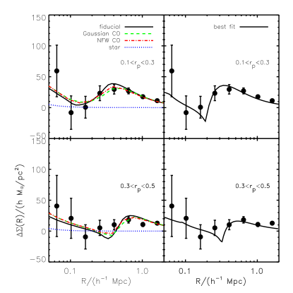
Figure 1: Solid dots show the measured excess surface density profiles, $\Delta\Sigma(R)$, around satellite galaxies in groups with assigned masses in the range $[10^{13},5\times 10^{14}]\,\rm{h^{-1}M_{\odot}}$. In the upper panels, the $r_{p}$ range of satellite galaxies is $[0.1,0.3]{\rm h^{-1}Mpc}$, while in the lower panels, the range is $[0.3,0.5]{\rm h^{-1}Mpc}$. Errorbars reflect the $68\%$ confidence intervals obtained using bootstrapping. The black solid lines in the left-hand panels show the predictions of our fiducial model (see §3), while the dashed and dash-dotted lines show the predictions using two different models for the center-offsets (see text for details). The blue dotted lines show the contribution of stellar component. The right-hand panels show the same data, but this time the solid lines correspond to the best-fit models described by Eq.(12). The corresponding best-fit parameters are listed in Table 1.

Figure 2: Solid dots show the measured $\Delta\Sigma(R)$ around central galaxies in groups with assigned masses in the range $[10^{13},5\times 10^{14}]\,\rm{h^{-1}M_{\odot}}$. Errorbars reflect the 1$\sigma$ uncertainties. The solid line corresponds to the excess surface density of the best-fit single NFW profile, which has a mass $\log(M/\rm{h^{-1}M_{\odot}})=13.32$, in excellent agreement with the average of the assigned halo masses of the groups, which is $\log(M/\rm{h^{-1}M_{\odot}})=13.37$.

4 Constraints on Model Parameters

Our theoretical predication given above is obtained by modeling halos and subhalos of individual satellites. In order to see how the observational data constrain the average mass of subhalos, we fit the data with a simple model assuming that the average lensing signal has the same form as a single lens system:

$$\Delta\Sigma=\Delta\Sigma_{\rm host}(R|M,r_{p})+\Delta\Sigma_{\rm sub}(R|M_{\rm sub},\rho_{\rm 0,sub},r_{\rm s,sub})\,.$$ (12)

Since the lensing signal of the stellar component is much smaller than that from dark matter subhalo, we ignore this component for simplicity. The model is therefore described by 5 free parameters: the host halo mass, $M$; the projected halo-centric distance $r_{p}$; the subhalo mass $M_{\rm sub}$; the subhalo characteristic density $\rho_{\rm 0,sub}$; and the subhalo scale radius $r_{\rm s,sub}$. For simplicity, the concentration of the host halo is fixed using the concentration-mass relation of Neto et al. (2007). We also ignore the center-offset here because it does not affect the lensing signal significantly. As in L13, we fit the data using a Monte Carlo Markov Chain (MCMC) method provided by the COSMOMC package (Lewis & Bridle, 2002). The best-fit results are shown in the right-hand panels of Fig. 1. In order to illustrate the typical uncertainties and degeneracies among the various parameters, Figs. 3 and 4 show the joint constraints on a subset of parameter pairs for satellites in the $r_{p}=[0.1,0.3]\,{\rm h^{-1}Mpc}$ bin. The best-fit value for the subhalo mass is $\log(M_{\rm sub}/\rm{h^{-1}M_{\odot}})=11.68\pm 0.67$, which is in excellent agreement with the average subhalo mass, $\langle\log{M_{\rm sub,theory}/\rm{h^{-1}M_{\odot}}}\rangle=11.30$, assigned to the satellite galaxies according to the model described in §3. Due to the limited data, however, the constraint is not particularly tight. In particular, the 95% confidence interval for $M_{\rm sub}$ covers the entire range $\log(M_{\rm sub}/\rm{h^{-1}M_{\odot}})=[9.0,12.5]$ In the case of the parameters $\rho_{\rm 0,sub}$ and $r_{\rm s,sub}$, no meaningful constraints can be obtained due the limited amount and quality of the data on small scales. The results for the $r_{p}=[0.3,0.5]\,{\rm h^{-1}Mpc}$ bin are similar. The best-fit values for $M$, $r_{p}$ and $M_{\rm sub}$ are listed in Table 1. Note that the best-fit value for the host halo mass, $M_{\rm fit}\sim 10^{13.7}\rm{h^{-1}M_{\odot}}$, is significantly larger than the average mass obtained directly from the SDSSGC ($10^{13.37}\rm{h^{-1}M_{\odot}}$) or from the lensing signal around the centrals ($10^{13.32}\rm{h^{-1}M_{\odot}}$; see Fig. 2). However, this arises because $M_{\rm fit}$ is weighted by the number of satellite galaxies per host. Since more massive groups host more satellites, on average, this weighting biases the inferred host halo high (cf. More, van den Bosch & Cacciato, 2009). Indeed, if we use the group catalogue to compute the satellite-weighted average host halo mass, we obtain the values listed in the fourth column of Table 1, which are in much better agreement with the best-fit value for $M_{\rm fit}$.

In the group catalog, some galaxies that are identified as satellite galaxies may actually be centrals of other (mostly low-mass) haloes along the line of sight. These galaxies, which we refer to as interlopers, produce contaminations to the total lensing signal. In Li13, the effect of interlopers was investigated with the mock group catalogue given in Yang et al. (2007) (for more details, see Sec.6.2 in L13). Using the same method, we find that the fraction of interlopers in the groups used here is 13%. The bias produced by the interlopers in the estimated subhalo mass is $\sim 0.1$ dex, much smaller than the statistical errors.

Table 1: The best-fit values of model parameters and our theoretical predictions. $N_{\rm sat}$ is the number of satellites used as lenses. $\langle\log M_{*}\rangle$ is the average stellar mass of the satellites. $\langle\log{M_{\rm theory}}\rangle$ is the average, satellite-weighted host halo mass predicted directly from the galaxy group catalog. $\langle\log{M_{\rm sub,theory}}\rangle$ is the mean subhalo mass expected from our theoretical model (§ 3). $\log{M_{\rm fit}}$, $r_{\rm p,fit}$ and $\log{M_{\rm sub,fit}}$ are the best-fit values for $M$, $r_{p}$ and $M_{\rm sub}$ obtained using the model described in § 4. All errors indicate the 68% confidence intervals. Finally, $\chi^{2}_{\rm red}$ is the reduced $\chi^{2}$ of the best-fit model. Masses and distances are in units of $\rm{h^{-1}M_{\odot}}$ and ${\rm h^{-1}Mpc}$, respectively.

Satellite $r_{p}$ range	$N_{\rm sat}$	$\langle\log(M_{*})\rangle$	$\langle\log{M_{\rm theory}}\rangle$	$\log{M_{\rm fit}}$	$r_{\rm p,fit}$	$\langle\log{M_{\rm sub,theory}}\rangle$	$\log{M_{\rm sub,fit}}$	$\chi^{2}_{\rm red}$
$[0.1,0.3]$	595	10.51	13.67	13.73 $\pm$ 0.04	0.19$\pm$ 0.01	11.30	11.68$\pm$ 0.67	1.68
$[0.3,0.5]$	475	10.52	13.78	13.50 $\pm$ 0.08	0.33 $\pm$ 0.04	11.23	11.68$\pm$ 0.76	1.02

Figure 3: The 68% and 95% confidence intervals for parameters $M$, $r_{p}$ and $M_{\rm sub}$. The last panel in each row shows the marginalized posterior distribution. The $r_{p}$ range of satellite galaxies is $[0.1,0.3]{\rm h^{-1}Mpc}$.

Figure 4: Similar to Fig. 3, but here the 68% and 95% confidence intervals are shown for parameters $M_{\rm sub}$, $\rho_{\rm 0,sub}$ and $r_{\rm s,sub}$.

5 Summary

We have used the Yang et al. (2007) galaxy group catalog constructed from the SDSS spectroscopic survey to select satellite galaxies and obtained tangential shears around them using sources selected from the CS82. This has resulted in a direct measurement of the gravitational lensing effect due to dark matter subhalos associated with satellite galaxies. Compared with previous studies based on massive clusters of galaxies (e.g. Natarajan, De Lucia & Springel, 2007; Natarajan et al., 2009), our results present the first measurement of the subhalo masses of satellites in galaxy groups.

The lensing effect is measured for satellites in groups with masses in the range $[10^{13},5\times 10^{14}]\rm{h^{-1}M_{\odot}}$, and the results agree well with theoretical expectations, although the errorbars are quite large, especially on small scales. Fitting the data points with a truncated NFW profile, we obtain an average subhalo mass of $\log(M_{\rm sub}/\rm{h^{-1}M_{\odot}})=11.68\pm 0.67$ for satellites located at projected group-centric distances in the range $[0.1,0.3]{\rm h^{-1}Mpc}$, and $\log(M_{\rm sub}/\rm{h^{-1}M_{\odot}})=11.68\pm 0.78$ for those in the range $[0.3,0.5]{\rm h^{-1}Mpc}$. The current data is still insufficient to put any meaningful constraints on the central density, $\rho_{\rm 0,sub}$, and/or scale radius, $r_{\rm s,sub}$, of subhalos. The best-fit subhalo masses are consistent (within the errors) with the truncated subhalo masses assigned to satellite galaxies using abundance matching. Our results prove the feasibility of using galaxy-galaxy weak lensing to study the properties of subhalos, once a well-defined galaxy group catalog is available to pre-select satellite galaxies. As discussed in L13, with next generation weak lensing surveys, which will yield many more source galaxies behind many more foreground galaxy groups, one will be able to constrain both the mass and the structure of subhalos associated with satellite galaxies in narrow bins of host halo mass bins and group-centric distance, $r_{p}$. This will yield constraints on the formation and evolution of dark matter subhalos, and perhaps even on the nature of the dark matter through its impact on the formation of cosmic structure on small scales.

References

- Abazajian et al. (2009) Abazajian K. N., Adelman-McCarthy J. K., Agüeros M. A., Allam S. S., Allende Prieto C., An D., Anderson K. S. J., 2009, ApJS, 182, 543
- Bell et al. (2003) Bell E. F., McIntosh D. H., Katz N., Weinberg M. D., 2003, ApJS, 149, 289
- Binney & Tremaine (1987) Binney J., Tremaine S., 1987, Galactic dynamics
- Brainerd, Blandford & Smail (1996) Brainerd T. G., Blandford R. D., Smail I., 1996, ApJ, 466, 623
- Buote et al. (2002) Buote D. A., Jeltema T. E., Canizares C. R., Garmire G. P., 2002, ApJ, 577, 183
- Cacciato et al. (2009) Cacciato M., van den Bosch F. C., More S., Li R., Mo H. J., Yang X., 2009, MNRAS, 394, 929
- Comparat et al. (2013) Comparat J. et al., 2013, ArXiv e-prints
- Erben et al. (2009) Erben T., Hildebrandt H., Lerchster M., Hudelot P., Benjamin J., van Waerbeke L., Schrabback T., Brimioulle F., 2009, A&A, 493, 1197
- Erben et al. (2013) Erben T., Hildebrandt H., Miller L., van Waerbeke L., Heymans C., Hoekstra H., Kitching T. D., Mellier Y., 2013, MNRAS, 433, 2545
- Gao et al. (2004) Gao L., White S. D. M., Jenkins A., Stoehr F., Springel V., 2004, MNRAS, 355, 819
- George et al. (2012) George M. R., Leauthaud A., Bundy K., Finoguenov A., Ma C.-P., Rykoff E. S., Tinker J. L., Wechsler R. H., 2012, ApJ, 757, 2
- Gillis et al. (2013a) Gillis B. R., Hudson M. J., Erben T., Heymans C., Hildebrandt H., Hoekstra H., Kitching T. D., Mellier, 2013a, MNRAS, 431, 1439
- Gillis et al. (2013b) Gillis B. R., Hudson M. J., Hilbert S., Hartlap J., 2013b, MNRAS, 429, 372
- Heymans et al. (2012) Heymans C., Van Waerbeke L., Miller L., Erben T., Hildebrandt H., Hoekstra H., Kitching T. D., Mellier Y., 2012, MNRAS, 427, 146
- Hoekstra et al. (2003) Hoekstra H., Franx M., Kuijken K., Carlberg R. G., Yee H. K. C., 2003, MNRAS, 340, 609
- Hoekstra (2004) Hoekstra H., 2004, MNRAS, 347, 1337
- Hudson et al. (1998) Hudson M. J., Gwyn S. D. J., Dahle H., Kaiser N., 1998, ApJ, 503, 531
- Johnston et al. (2007) Johnston D. E., Sheldon E. S., Tasitsiomi A., Frieman J. A., Wechsler R. H., McKay T. A., 2007, ApJ, 656, 27
- Kneib et al. (1996) Kneib J.-P., Ellis R. S., Smail I., Couch W. J., Sharples R. M., 1996, ApJ, 471, 643
- Kneib & Natarajan (2011) Kneib J.-P., Natarajan P., 2011, A&ARv, 19, 47
- Kochanek & Dalal (2004) Kochanek C. S., Dalal N., 2004, ApJ, 610, 69
- Komatsu et al. (2010) Komatsu E., Smith K. M., Dunkley J., Bennett C. L., Gold B., Hinshaw G., Jarosik N., Larson D., 2010, ArXiv e-prints
- Koopmans (2005) Koopmans L. V. E., 2005, MNRAS, 363, 1136
- Leauthaud et al. (2012) Leauthaud A., Tinker J., Bundy K., Behroozi P. S., Massey R., Rhodes J., George M. R., Kneib J.-P., 2012, ApJ, 744, 159
- Lewis & Bridle (2002) Lewis A., Bridle S., 2002, PhRevD, 66, 103511
- Li et al. (2009) Li R., Mo H. J., Fan Z., Cacciato M., van den Bosch F. C., Yang X., More S., 2009, MNRAS, 394, 1016
- Li et al. (2013) Li R., Mo H. J., Fan Z., Yang X., Bosch F. C. v. d., 2013, MNRAS, 430, 3359
- Limousin et al. (2007) Limousin M., Kneib J. P., Bardeau S., Natarajan P., Czoske O., Smail I., Ebeling H., Smith G. P., 2007, A&A, 461, 881
- Limousin et al. (2009) Limousin M., Sommer-Larsen J., Natarajan P., Milvang-Jensen B., 2009, ApJ, 696, 1771
- Macciò & Miranda (2006) Macciò A. V., Miranda M., 2006, MNRAS, 368, 599
- Mandelbaum et al. (2005) Mandelbaum R. et al., 2005, MNRAS, 361, 1287
- Mandelbaum et al. (2006) Mandelbaum R., Seljak U., Kauffmann G., Hirata C. M., Brinkmann J., 2006, MNRAS, 368, 715
- Mandelbaum, Seljak & Hirata (2008) Mandelbaum R., Seljak U., Hirata C. M., 2008, JCAP, 8, 6
- Mao & Schneider (1998) Mao S., Schneider P., 1998, MNRAS, 295, 587
- Mao et al. (2004) Mao S., Jing Y., Ostriker J. P., Weller J., 2004, ApJL, 604, L5
- McKay et al. (2001) McKay T. A., Sheldon E. S., Racusin J., Fischer P., Seljak U., Stebbins A., Johnston D., Frieman J. A. a., 2001, ArXiv Astrophysics e-prints
- Metcalf & Madau (2001) Metcalf R. B., Madau P., 2001, ApJ, 563, 9
- Miller et al. (2007) Miller L., Kitching T. D., Heymans C., Heavens A. F., van Waerbeke L., 2007, MNRAS, 382, 315
- Miller et al. (2013) Miller L., Heymans C., Kitching T. D., van Waerbeke L., Erben T., Hildebrandt H., Hoekstra H., Mellier Y., 2013, MNRAS, 429, 2858
- More, van den Bosch & Cacciato (2009) More S., van den Bosch F. C., Cacciato M., 2009, MNRAS, 392, 917
- Natarajan, De Lucia & Springel (2007) Natarajan P., De Lucia G., Springel V., 2007, MNRAS, 376, 180
- Natarajan et al. (2009) Natarajan P., Kneib J.-P., Smail I., Treu T., Ellis R., Moran S., Limousin M., Czoske O., 2009, ApJ, 693, 970
- Navarro, Frenk & White (1997) Navarro J. F., Frenk C. S., White S. D. M., 1997, ApJ, 490, 493
- Neto et al. (2007) Neto A. F. et al., 2007, MNRAS, 381, 1450
- Pastor Mira et al. (2011) Pastor Mira E., Hilbert S., Hartlap J., Schneider P., 2011, A&A, 531, A169
- Prada et al. (2003) Prada F., Vitvitska M., Klypin A., Holtzman J. A., Schlegel D. J., Grebel E. K., Rix H.-W., Brinkmann J., 2003, ApJ, 598, 260
- Sheldon et al. (2009) Sheldon E. S. et al., 2009, ApJ, 703, 2217
- Skibba et al. (2011) Skibba R. A., van den Bosch F. C., Yang X., More S., Mo H., Fontanot F., 2011, MNRAS, 410, 417
- Sofue & Rubin (2001) Sofue Y., Rubin V., 2001, A&ARv, 39, 137
- Springel et al. (2008) Springel V., Wang J., Vogelsberger M., Ludlow A., Jenkins A., Helmi A., Navarro J. F., Frenk C. S., 2008, MNRAS, 391, 1685
- Tormen, Diaferio & Syer (1998) Tormen G., Diaferio A., Syer D., 1998, MNRAS, 299, 728
- van den Bosch, Tormen & Giocoli (2005) van den Bosch F. C., Tormen G., Giocoli C., 2005, MNRAS, 359, 1029
- van den Bosch et al. (2005) van den Bosch F. C., Weinmann S. M., Yang X., Mo H. J., Li C., Jing Y. P., 2005, MNRAS, 361, 1203
- Vegetti & Koopmans (2009a) Vegetti S., Koopmans L. V. E., 2009a, MNRAS, 392, 945
- Vegetti & Koopmans (2009b) Vegetti S., Koopmans L. V. E., 2009b, MNRAS, 400, 1583
- Vegetti et al. (2010) Vegetti S., Koopmans L. V. E., Bolton A., Treu T., Gavazzi R., 2010, MNRAS, 408, 1969
- Vegetti et al. (2012) Vegetti S., Lagattuta D. J., McKean J. P., Auger M. W., Fassnacht C. D., Koopmans L. V. E., 2012, Nature, 481, 341
- Wang (2013) Wang L., 2013, in preparation
- Xu et al. (2009) Xu D. D. et al., 2009, MNRAS, 398, 1235
- Yang et al. (2005) Yang X., Mo H. J., van den Bosch F. C., Jing Y. P., 2005, MNRAS, 356, 1293
- Yang et al. (2006) Yang X., Mo H. J., van den Bosch F. C., Jing Y. P., Weinmann S. M., Meneghetti M., 2006, MNRAS, 373, 1159
- Yang et al. (2007) Yang X., Mo H. J., van den Bosch F. C., Pasquali A., Li C., Barden M., 2007, ApJ, 671, 153
- Yang, Mo & van den Bosch (2008) Yang X., Mo H. J., van den Bosch F. C., 2008, ApJ, 676, 248