Collision Strengths for [O iii] Optical and Infrared Lines

Abstract

We present electron collision strengths and their thermally averaged values for the forbidden lines of the astronomically abundant doubly-ionized oxygen ion, O²⁺, in an intermediate coupling scheme using the Breit-Pauli relativistic terms as implemented in an R-matrix atomic scattering code. We use several atomic targets for the R-matrix scattering calculations including one with 72 atomic terms. We also compare with new results obtained using the intermediate coupling frame transformation method. We find spectroscopically significant differences against a recent Breit-Pauli calculation for the excitation of the [O iii] $\lambda$4363 transition but confirm the results of earlier calculations.

1 Introduction

The forbidden lines of O²⁺ are among the most important features in the spectra of photoionized plasmas which include, inter alia, H ii regions and planetary nebulae. The exceptional brightness of the strongest [O iii] lines means that they can be used to determine the oxygen abundances and physical conditions in the Milky Way and other galaxies out to cosmological distances that reach redshifts of more than $z=3$ (Maiolino et al, 2008).

It has been recently suggested (Nicholls et al, 2012) that the elemental abundance and electron temperature anomalies seen in the analysis of the planetary nebula spectra, where considerable differences have been observed between the results obtained from the collisionally-excited lines (CEL) and those obtained from the optical recombination lines (ORL), might be resolved by using non Maxwell-Boltzmann (MB) distributions for the energies of the free electrons. The $\kappa$ distribution, which is widely used in the analysis of solar data, was proposed as a replacement for the MB distribution to resolve this issue. If the electron distributions are generally non-Maxwellian in nebulae it would affect the analysis of [O iii] lines significantly and reliable collision strength data are needed to compute the effective collision strengths for collisional excitation and de-excitation.

The proposal that the electron energy distribution in planetary nebulae is not Maxwellian dates back to the 1940s at least where Hagihara (1944) proposed that the velocity distribution of free electrons in gaseous assemblies, such as those found in planetary nebulae, deviates significantly from the Maxwellian. Bohm & Aller (1947) argued against Hagihara and concluded that any deviation from the Maxwellian equilibrium distribution is very small. The essence of Bohm and Aller’s argument is that for typical planetary nebulae conditions of electron temperature of about 10000 K and electron number density of about $10^{4}$ cm^-3, the thermalization process of elastic collisions between an electron and other electrons and ions is by far the most frequent event and typically occurs once every second, while other processes that shift the system from its thermodynamic equilibrium, like inelastic scattering with other ions that leads to metastable excitation or recapture, occur at much larger time scales estimated to be months or even years. Bohm and Aller also indicated the significance of any possible deviation from a Maxwellian distribution on derived elemental abundances.

Although there have been many studies related to collision strengths of O²⁺, as we will discuss in the coming paragraphs, some of the previous data have limitations. For example, some of these data are produced in an $LS$ coupling scheme while others are based on approaches that do not adequately treat resonance phenomena.

Before the advent of close-coupling codes there were several calculations of collision strengths for excitation of the O iii forbidden lines that did not incorporate resonance effects (Czyzak et al, 1968; Seaton, 1975; Bhatia et al, 1979).

The first close-coupled collision strengths were obtained by Baluja et al (1980) for some of the semi-forbidden intercombination transitions of O iii using the R-matrix method (Berrington et al, 1974, 1987; Hummer et al, 1993; Berrington et al, 1995). They included all channels with configurations 1s² 2s² 2p², 1s² 2s 2p³ and 1s² 2p⁴ in the expansion of the wavefunction. They also used three pseudo-orbitals ($\overline{3}\rm{s}$, $\overline{3}\rm{p}$ and $\overline{3}\rm{d}$) and allowed for configuration interaction in the included states with the addition of correlation terms in the total wavefunction.

Ho & Henry (1983) also used the close coupling approximation with configuration interaction in the target wavefunction to compute the collision strengths of some of O iii transitions in $LS$ coupling. They employed a mix of spectroscopic and correlation Hartree-Fock orbitals to describe their target.

Relatively extensive work was done by Aggarwal (1983, 1985) who computed collision strengths of O iii transitions between the fine structure levels using configuration interaction target wavefunctions. He transformed $LS$ coupling reactance matrices obtained from R-matrix calculations to pair coupling with the program JAJOM (Saraph, 1978). The results were obtained with a fine energy mesh up to 5.16 Rydberg where a complex resonance structure was observed on the entire mesh.

Aggarwal (1993) used an elaborate configuration interaction target described by Aggarwal & Hibbert (1991) and the R-matrix method in $LS$ coupling to compute effective collision strengths for some inelastic transitions of O iii between 26 $LS$-coupled states of six configurations over a wide range of electron temperature (2500-200000 K). They employed the standard and no-exchange R-matrix codes on a fine energy mesh that reveals the resonance structure. This work was extended by Aggarwal & Keenan (1999), who they computed the collision strengths for the transitions between the fine structure levels using the R-matrix method including all partial waves with $L\leq 40$ to ensure convergence. Aggarwal & Keenan (1999) transformed the $LS$ reactance matrices obtained by Aggarwal (1993) into pair coupling using JAJOM (Saraph, 1978) where necessary. They only tabulated fine-structure collision strengths for some transitions, pointing out that in pair coupling, if one of the terms in a transition has spin zero and hence $J=L$, e.g. ³P – ¹D, the fine-structure collision strengths are proportional to the statistical weight of the non-zero spin states, in this example the ³P_J levels.

Lennon & Burke (1994) did extensive work on O²⁺ collision strengths for the transitions between the fine structure levels, as part of a wider investigation on the carbon isoelectronic ions, using the R-matrix method, where the CIV3 configuration interaction code (Hibbert, 1975) was used to generate the target wavefunctions. The target included 12 states belonging to 3 configurations (1s² 2s² 2p², 1s² 2s 2p³ and 1s² 2p⁴). They also transformed to pair coupling in the same way as Aggarwal & Keenan (1999) described above. They presented a sample of Maxwellian based effective collision strengths in the temperature range $10^{3}-10^{5}$ K.

Recently, Palay et al (2012) made the first calculation of collision strengths for the O iii forbidden transitions using a relativistic Breit-Pauli (BP) R-matrix method with resolved resonance structures. They used 22 configurations (3 spectroscopic and 19 correlation) to describe the target. Like most of the previous studies, they have also presented samples of the Maxwellian averaged effective collision strengths which were also computed at temperatures down to 100 K.

The most recent R-matrix calculations (Lennon & Burke, 1994; Aggarwal & Keenan, 1999; Palay et al, 2012) generally agree to within 10% for the thermally averaged collision strengths for the forbidden transitions among the five lowest levels. An exception to this generally close agreement is for the transitions from the lowest three ³P_J levels to the ¹S₀ state. The recent results of Palay et al (2012) differ significantly from those of earlier workers. The excitation mechanism of the ¹S₀ level is important because the ¹S${}_{0}\rightarrow^{1}$D₂ $\lambda 4363$ line is widely used to infer the electron temperature in H ii regions and planetary nebulae. If a $\kappa$ distribution of electron energies is assumed, the number of free electrons capable of exciting the ¹S₀ state would be increased relative to a MB distribution which would affect the derived O²⁺ abundance.

The aim of the present paper is twofold. Firstly we make a Breit-Pauli R-matrix calculation of the O²⁺ collision strengths with an independently derived target configuration basis to compare with previous work, especially the only other Breit-Pauli results from Palay et al (2012). Secondly we attempt to place realistic error estimates on our results by examining the effect of several factors on our results. We discuss the convergence of our calculation as the number of target states is increased. Our largest target includes significant contributions to the dipole polarizability of the three energetically lowest terms. We also consider the effect of Gailitis averaging of the collision strengths close to the excitation thresholds, especially for excitation of the ³P₁ level between the ³P₁ and ³P₂ thresholds. We additionally compare the results of the Breit-Pauli calculation with those obtained using the Intermediate Coupling Frame Transformation (ICFT) R-matrix method (Griffin, Badnell & Pindzola, 1998). This method is based on transforming the non-physical $LS$-coupled reactance matrices, to compute collision strengths in intermediate coupling.

The calculation described in the following sections is constructed to provide accurate results for the excitation of the optical and infrared forbidden transitions among the five lowest levels of O²⁺ at temperatures typical of photoionized plasmas. We compute collision strengths up to $\approx 1.3$ Rydberg free electron energy relative to the ground level and Mawell-Boltzmann averaged collision strengths from 100 K to 25000 K.

The main tools used in this investigation are the Autostructure code (Eissner et al, 1974; Nussbaumer & Storey, 1978; Badnell, 2011) to define and elaborate the atomic target and the UCL-Belfast-Strathclyde R-matrix code (Berrington et al, 1995) to do the actual scattering calculations. We compare our results with earlier calculations and also assess the reliability of our results.

2 Computation

In the following we outline the computational methods used in this work.

2.1 The O²⁺ target

We used the Autostructure code (Badnell, 2011) to generate the target radial functions required as an input to the first stage of the R-matrix code. The radial data were generated using thirty-nine configurations containing seven orbitals; three physical (1s, 2s and 2p) and four correlation orbitals ($\overline{3}\rm{s}$, $\overline{3}\rm{p}$, $\overline{3}\rm{d}$, $\overline{4}\rm{f}$). These configurations are given in Table 1. An iterative optimization variational protocol was used to obtain the orbital scaling parameters, $\lambda_{nl}$, which are given in Table 2. The correlation orbitals are calculated in a Coulomb potential with central charge 8$|\lambda_{nl}|$.

Table 1: The configuration basis used to define the scattering target. The 1s² core is to be understood in all configurations. The bar signifies a correlation orbital.

2s2 2p2, 2s 2p3, 2p4

2s2 2p $\overline{3}{l}$; $l=0,1,2$

2s 2p2 $\overline{3}{l}$; $l=0,1,2$

2p3 $\overline{3}{l}$; $l=0,1,2$

2s2 $\overline{3}{l}$ $\overline{3}{l}^{{}^{\prime}}$, $l,l^{{}^{\prime}}$=0,1,2

2s 2p $\overline{3}{l}$ $\overline{3}{l}^{{}^{\prime}}$, $l,l^{{}^{\prime}}$=0,1,2

2p2 $\overline{3}{l}$ $\overline{3}{l}^{{}^{\prime}}$, $l,l^{{}^{\prime}}$=0,1,2

2s2 2p $\overline{4}\rm{f}$, 2s 2p2 $\overline{4}\rm{f}$, 2p3 $\overline{4}\rm{f}$

2s2 $\overline{3}\rm{d}$ $\overline{4}\rm{f}$, 2s 2p $\overline{3}\rm{d}$ $\overline{4}\rm{f}$, 2p2 $\overline{3}\rm{d}$ $\overline{4}\rm{f}$

2s2 $\overline{4}\rm{f}^{2}$, 2s 2p $\overline{4}\rm{f}^{2}$, 2p2 $\overline{4}\rm{f}^{2}$

Table 2: Orbital scaling parameters, $\lambda_{nl}$, for Autostructure input. The rows stand for the principal quantum number $n$, while the columns stand for the orbital angular momentum quantum number $l$.

	s	p	d	f
1	1.44889
2	1.22418	1.18282
$\overline{3}$	-0.80508	-0.61905	-1.04731
$\overline{4}$				-1.87410

Table 3: Target terms and energies, $E$, calculated by Autostructure using the configuration basis listed in Table 1. The 1s² core is suppressed from all configurations. All these terms are included in the 72-term target, while for the smaller targets (10- and 20-term) only the first 10 and 20 terms respectively are included.

Index	Configuration	Term	$E$ (cm-1)	Index	Configuration	Term	$E$ (cm-1)
1	2s2 2p2	3Pe	0.0	37	2s 2p2 $\overline{3}\rm{p}$	1So	483995
2	2s2 2p2	1De	21257	38	2s 2p2 $\overline{3}\rm{p}$	3Po	485363
3	2s2 2p2	1Se	45630	39	2s 2p2 $\overline{3}\rm{s}$	3Se	486363
4	2s 2p3	5So	58948	40	2s 2p2 $\overline{3}\rm{p}$	1Po	486594
5	2s 2p3	3Do	121133	41	2s 2p2 $\overline{3}\rm{p}$	3Do	491627
6	2s 2p3	3Po	144640	42	2s 2p2 $\overline{3}\rm{s}$	3Pe	496357
7	2s 2p3	1Do	190314	43	2s 2p2 $\overline{3}\rm{p}$	3Po	498566
8	2s 2p3	3So	199693	44	2s 2p2 $\overline{3}\rm{p}$	3So	503468
9	2s 2p3	1Po	214885	45	2s 2p2 $\overline{3}\rm{s}$	1Pe	506149
10	2p4	3Pe	287613	46	2s 2p2 $\overline{3}\rm{s}$	1Se	508564
11	2s2 2p $\overline{3}\rm{p}$	1Pe	301182	47	2s 2p2 $\overline{3}\rm{p}$	1Do	509665
12	2p4	1De	302782	48	2s 2p2 $\overline{3}\rm{p}$	1Po	526999
13	2s2 2p $\overline{3}\rm{p}$	3De	306265	49	2s2 2p $\overline{3}\rm{d}$	3Fo	539361
14	2s2 2p $\overline{3}\rm{s}$	3Po	309248	50	2p3 $\overline{3}\rm{p}$	5Pe	542552
15	2s2 2p $\overline{3}\rm{p}$	3Se	310788	51	2s2 2p $\overline{3}\rm{d}$	1Do	550865
16	2s2 2p $\overline{3}\rm{p}$	3Pe	315730	52	2p3 $\overline{3}\rm{s}$	5So	551832
17	2s2 2p $\overline{3}\rm{s}$	1Po	323156	53	2p3 $\overline{3}\rm{p}$	3Pe	553504
18	2s2 2p $\overline{3}\rm{p}$	1De	328464	54	2p3 $\overline{3}\rm{p}$	3De	567272
19	2s2 2p $\overline{3}\rm{p}$	1Se	345567	55	2p3 $\overline{3}\rm{p}$	1Pe	567946
20	2p4	1Se	351203	56	2p3 $\overline{3}\rm{p}$	3Fe	568179
21	2s 2p2 $\overline{3}\rm{p}$	3So	372370	57	2p3 $\overline{3}\rm{p}$	1Fe	570684
22	2s 2p2 $\overline{3}\rm{p}$	5Do	376169	58	2s2 2p $\overline{3}\rm{d}$	3Po	572129
23	2s 2p2 $\overline{3}\rm{s}$	5Pe	379161	59	2s2 2p $\overline{3}\rm{d}$	3Do	578854
24	2s 2p2 $\overline{3}\rm{p}$	5Po	379976	60	2p3 $\overline{3}\rm{s}$	3Do	584855
25	2s 2p2 $\overline{3}\rm{p}$	3Do	392038	61	2p3 $\overline{3}\rm{s}$	3So	589631
26	2s 2p2 $\overline{3}\rm{p}$	5So	395094	62	2p3 $\overline{3}\rm{p}$	3Pe	600736
27	2s 2p2 $\overline{3}\rm{p}$	3Po	400796	63	2s 2p2 $\overline{3}\rm{d}$	5Fe	600824
28	2s 2p2 $\overline{3}\rm{s}$	3Pe	418063	64	2p3 $\overline{3}\rm{s}$	1Do	602294
29	2s 2p2 $\overline{3}\rm{p}$	3Fo	437947	65	2p3 $\overline{3}\rm{p}$	1De	606079
30	2s 2p2 $\overline{3}\rm{p}$	1Do	439915	66	2p3 $\overline{3}\rm{p}$	3Se	606299
31	2s 2p2 $\overline{3}\rm{s}$	3De	442045	67	2p3 $\overline{3}\rm{p}$	3De	607292
32	2s 2p2 $\overline{3}\rm{p}$	1Fo	443431	68	2s 2p2 $\overline{3}\rm{d}$	5De	610073
33	2s 2p2 $\overline{3}\rm{p}$	3Do	447068	69	2p3 $\overline{3}\rm{p}$	1Pe	612417
34	2s 2p2 $\overline{3}\rm{p}$	1Po	449383	70	2s2 2p $\overline{3}\rm{d}$	1Po	617417
35	2s 2p2 $\overline{3}\rm{p}$	3Po	456397	71	2p3 $\overline{3}\rm{p}$	3Pe	618955
36	2s 2p2 $\overline{3}\rm{s}$	1De	468076	72	2s2 2p $\overline{3}\rm{d}$	1Fo	620437

In the scattering calculations, targets with differing numbers of target states were used, with the largest having 72 terms which are listed in Table 3. Calculations were also made with the first 10 and 20 terms from this list as discussed in more detail below.

In Table 4 we show the statistically weighted oscillator strengths, $gf$, in the length and velocity formulations for all the strong allowed transitions between the 2s² 2p² and 2s 2p³ configurations. The agreement is excellent. Good agreement between the length and velocity results is a necessary but not sufficient condition for ensuring the quality of the target wave functions. These transitions also make the largest contributions to the dipole polarizabilities of the three lowest terms.

The 72 terms listed in Table 3 were chosen to include all those correlation configurations that contribute significantly to the dipole polarizability of the three lowest terms. The main contributions come from 2s² 2p $\overline{3}\rm{d}$ configuration. The contribution of states outside the $n=2$ complex to the dipole polarizabilities of the ³P, ¹D and ¹S terms is 37%, 37% and 60% respectively. In Table 5 we list the energies of the 18 levels of the $n=2$ complex configurations. We show theoretical energies which include one- and two-body fine-structure interactions ($E{{}_{\rm{th2}}}$) and those which only include the spin-orbit interaction ($E{{}_{\rm{th1}}}$), the latter being the only fine-structure interactions included in the version of the R-matrix code that we use (see footnote 2). We return to the effect of omitting two-body fine structure interactions in section 3.

2.2 The Scattering Calculations

We made several calculations with increasing numbers of target states, both with Breit-Pauli and the Intermediate Coupling Frame Transformation R-matrix methods. The target radial functions were supplied as a radial grid format rather than Slater type orbital format where the radial file was generated by Autostructure. The inner region radius (RA) in the R-matrix formulation was 9.315 au. Twelve continuum basis functions were used to represent the wavefunctions in the inner region. This choice was based on convergence tests and with experience from previous work on the C⁺+e system (Sochi, 2012; Sochi & Storey, 2013). The maximum value of $2J$ for the $(N+1)$-electron problem was chosen to be 19 although 15 was found to be sufficient for convergence of the collision strengths for the forbidden transitions of interest here.

As indicated previously, we made three sets of calculations using the configuration basis described in section 2.1 with 10-, 20- and 72-terms using both the BP and ICFT approaches. These three targets comprise 18, 34 and 146 fine-structure levels respectively. The main purpose of using several targets is to have an estimate of the error in the final results from observing the convergence of the results with different numbers of target terms. For all three targets, the $(N+1)$-electron wavefunction contains all possible configurations formed from the 39 configurations of the $N$-electron target combined with any of the orbitals, spectroscopic and correlation. There are 102 such $(N+1)$-electron configurations.

Experimental energies obtained from the National Institute of Standards and Technology (NIST) were used in place of theoretical ones to ensure correct positioning of thresholds for convergence of resonance series. In some cases this required re-ordering the target states.

Table 4: The weighted $LS$ oscillator strengths in length, $(gf)_{{}_{L}}$, and velocity, $(gf)_{{}_{V}}$, forms for the transitions within the $n=2$ complex.

		$(gf)_{{}_{L}}$	$(gf)_{{}_{V}}$
3Pe	3Do	1.01	0.99
	3Po	1.28	1.31
	3So	1.70	1.61
1De	1Do	1.57	1.61
	1Po	1.18	1.22
1Se	1Po	0.27	0.27

Table 5: The 18 lowest energy levels of O²⁺ and their experimental ($E_{\rm{ex}}$) and theoretical ($E{{}_{\rm{th1}}}$ and $E{{}_{\rm{th2}}}$) energies in wavenumbers (cm^-1). The experimental energies are obtained from the NIST database while the theoretical energies were obtained from Autostructure with the configuration basis listed in Table 1. The energies $E{{}_{\rm{th1}}}$ were obtained with only spin-orbit terms in the target Hamiltonian while $E{{}_{\rm{th2}}}$ also include two-body fine-structure interactions within the $n=2$ complex.

Index	Level	$E_{\rm{ex}}$	$E{{}_{\rm{th1}}}$	$E{{}_{\rm{th2}}}$
1	2s2 2p2 3P${}^{\rm{e}}_{{}_{0}}$	0.00	0	0
2	2s2 2p2 3P${}^{\rm{e}}_{{}_{1}}$	113.18	115	113
3	2s2 2p2 3P${}^{\rm{e}}_{{}_{2}}$	306.17	339	308
4	2s2 2p2 1D${}^{\rm{e}}_{{}_{2}}$	20273.27	21489	21471
5	2s2 2p2 1S${}^{\rm{e}}_{{}_{0}}$	43185.74	45900	45882
6	2s 2p3 5S${}^{\rm{o}}_{{}_{2}}$	60324.79	59600	59582
7	2s 2p3 3D${}^{\rm{o}}_{{}_{3}}$	120058.2	121800	121775
8	2s 2p3 3D${}^{\rm{o}}_{{}_{2}}$	120053.4	121804	121799
9	2s 2p3 3D${}^{\rm{o}}_{{}_{1}}$	120025.2	121812	121805
10	2s 2p3 3P${}^{\rm{o}}_{{}_{2}}$	142393.5	145316	145307
11	2s 2p3 3P${}^{\rm{o}}_{{}_{1}}$	142381.8	145321	145307
12	2s 2p3 3P${}^{\rm{o}}_{{}_{0}}$	142381.0	145331	145319
13	2s 2p3 1D${}^{\rm{o}}_{{}_{2}}$	187054.0	191025	191006
14	2s 2p3 3S${}^{\rm{o}}_{{}_{1}}$	197087.7	200423	200405
15	2s 2p3 1P${}^{\rm{o}}_{{}_{1}}$	210461.8	215609	215591
16	2p4 3P${}^{\rm{e}}_{{}_{2}}$	283759.7	288653	288629
17	2p4 3P${}^{\rm{e}}_{{}_{1}}$	283977.4	288863	288854
18	2p4 3P${}^{\rm{e}}_{{}_{0}}$	284071.9	288965	288951

(a) 1-2

(b) 1-3

(c) 1-4

Figure 1: Collision strength (vertical axis) versus final electron energy in Rydberg (horizontal axis) for Breit-Pauli calculations of the 1-2, 1-3 and 1-4 transitions with 10-term (dotted), 20-term (dashed), and 72-term (solid). Refer to Table 5 for level indexing.

Collision strengths were calculated for electron energies up to 1.28 Rydberg relative to the 2s² 2p^2 3P${}^{\rm{e}}_{{}_{0}}$ ground level, hence 0.89 Rydberg relative to the highest state of interest, 2s² 2p^2 1S${}^{\rm{e}}_{{}_{0}}$. This energy corresponds to $\approx 7kT$ when the electron temperature $T=20000$ K, the approximate upper limit for temperatures in photoionized nebulae. Over this energy range, collision strengths were calculated at 20000 equally spaced energies, except between the 2s² 2p^2 3P${}^{\rm{e}}_{{}_{1}}$ and ³P${}^{\rm{e}}_{{}_{2}}$ levels where calculations were performed on a mesh 100 times finer. Calculations were also made with and without Gailitis averaging of the collision strengths in the region beneath each threshold where the effective quantum number $\nu>10$.

We calculate the thermodynamically-averaged collision strengths for electron excitation, $\Upsilon$, from a lower state $i$ to an upper state $j$ from

$$\Upsilon_{i\rightarrow j}\left(\epsilon_{i},T_{\rm f}\right)=\frac{\sqrt{\pi}}{2}e^{\left(\frac{\Delta E_{ij}}{kT_{\rm f}}\right)}\int_{0}^{\infty}\Omega_{ij}\left(\epsilon_{i}\right)\left(\frac{kT_{\rm f}}{\epsilon_{i}}\right)^{1/2}f\left(\epsilon_{i},T_{\rm f}\right)d\epsilon_{j}$$ (1)

where $T_{\rm f}$ is the effective temperature, $k$ is the Boltzmann constant, $\epsilon_{i}$ and $\epsilon_{j}$ are the free electron energy relative to the states $i$ and $j$ respectively, $\Delta E_{ij}$ ($=\epsilon_{j}-\epsilon_{i}$) is the energy difference between the two states, $\Omega_{ij}$ is the collision strength of the transition between the $i$ and $j$ states, and $f(\epsilon_{i},T_{\rm f})$ is the energy- and temperature-dependent electron distribution. In what follows we will only consider Maxwell-Boltzmann distributions of electron energy, given by

$$f_{{\rm MB}}(\epsilon,T)=\frac{2}{\left(kT\right)^{3/2}}\sqrt{\frac{\epsilon}{\pi}}e^{-\frac{\epsilon}{kT}},$$ (2)

although, as discussed above, other distributions such as the $\kappa$ distribution have been proposed and discussed (Vasyliunas, 1968; Nicholls et al, 2012; Storey & Sochi, 2013).

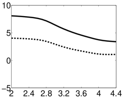
(a) 1-2

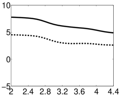
(b) 1-3

(c) 1-4

(d) 1-5

(e) 2-3

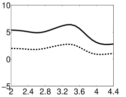
(f) 2-4

(g) 2-5

(h) 3-4

(i) 3-5

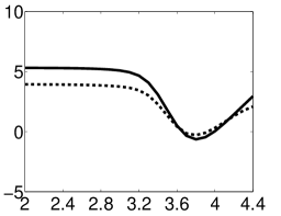
(j) 4-5

Figure 2: Thermally averaged collision strengths from the 10-term target (solid line) and 20-term target (dotted line), shown as the percentage difference from the 72-term target, plotted against log $T$ [K]. The labels of the sub-figures refer to the level indices in Table 5.

3 Results and Discussion

3.1 Results

A sample of our 10-, 20- and 72-term BP collision strengths is shown in Figure 1. The agreement between the three calculations is excellent, with the most obvious difference being that some resonances move to lower energies as the target size is increased, as might be expected. Figure 2 shows the results for the thermally averaged collision strength, $\Upsilon$, as a function of temperature for the 10- and 20-term calculations relative to the 72-term calculation as a percentage difference. The differences are less than 9% at any temperature for the 10-term calculation and less than 5% for the 20-term case.

The energy region between the 2s² 2p^2 3P${}^{\rm{e}}_{{}_{1}}$ and ³P${}^{\rm{e}}_{{}_{2}}$ states contains a Rydberg series of resonances converging on the ³P${}^{\rm{e}}_{{}_{2}}$ level with an effective quantum number at the ³P${}^{\rm{e}}_{{}_{1}}$ threshold of $47.7$. The energy difference between the ³P${}^{\rm{e}}_{{}_{1}}$ and ³P${}^{\rm{e}}_{{}_{2}}$ levels of 193 cm^-1 corresponds to a temperature of 278 K, so this energy region is significant for computing $\Upsilon$ at temperatures down to 100 K. We calculate the collision strengths with an energy interval of $6.4\times 10^{-7}$ Rydberg in this interval and compare with the result of using Gailitis averaging in this region. The difference is less than 1% at any temperature and we conclude that Gailitis averaging is adequate to obtain accurate values of $\Upsilon$ down to 100 K.

Figure 3: Effective collision strength (Upsilon) versus temperature from the 72-term target: Breit-Pauli (solid line), ICFT before modification (dotted line) and ICFT after modification (dashed line), for the transition between levels 2 and 3 of Table 5. On this scale the solid and dashed lines are almost indistinguishable.

The results of the ICFT calculations showed unexpectedly large differences from the BP results in some energy domains. This is illustrated in Figure 3 where we compare the thermally averaged collision strengths for the 72-term ICFT calculations with the 72-term BP results for the ³P${}^{\rm{e}}_{{}_{1}}$ – ³P${}^{\rm{e}}_{{}_{2}}$ transition. Due to the difference in scaling with effective charge ($z_{\rm eff}$) of term energy separations ($\propto z_{\rm eff}$) and resonance energies ($\propto z_{\rm eff}^{2}$), resonance effective quantum numbers can become small for lowly ionized systems. Such deeply-closed channels can be problematic for the multi-channel quantum defect theory (MQDT) used by the ICFT method due to computational finite numerical precision of highly divergent wavefunctions. Gorczyca & Badnell (2000) found that classically forbidden channels (e.g. $n<l$) could be handled expediently by simply omitting them from the MQDT representation. For low-energy scattering in O²⁺ we encountered a similar problem in a new guise for $n\lesssim 2$. The closed-channel partition of the MQDT representation should give no contribution since all bound orbitals (spectroscopic and pseudo) are projected out of the continuum basis. All such closed channel contributions (e.g. correlation resonances) arise instead in the open-open part of the scattering matrix. For $l>1$ the original Gorczyca & Badnell (2000) expediency already omits such closed channels ($n<l$). For $l=0,1$ we found it necessary to explicitly omit such closed channels from the closed partition as well. We show the effect of this modification as the dashed line in Figure 3. The agreement with the full Breit-Pauli calculation is now excellent.

Considering the convergence as the number of target states is increased and the good agreement between the ICFT and Breit-Pauli results, we adopt the results of the 72-term Breit-Pauli calculation as our final results and, based on the convergence behavior and the effect of Gailitis averaging, estimate an uncertainty of no more than 5% in the final thermally averaged collision strengths. In Table 6 we tabulate thermally averaged collision strengths $\Upsilon$, for the 72-term target in the temperature range log${}_{10}T$ = 2.0(0.1)4.4.

Table 6: Thermally averaged collision strengths from the 72-term Breit-Pauli calculation as a function of temperature. The transitions are indexed as in Table 5.

log $T$ [K]	1-2	1-3	1-4	1-5	2-3	2-4	2-5	3-4	3-5	4-5
2.0	0.63500	0.22586	0.23177	0.02989	1.11212	0.69748	0.09003	1.17021	0.15117	0.38267
2.1	0.62649	0.22561	0.23211	0.02989	1.10993	0.69849	0.09003	1.17188	0.15116	0.38291
2.2	0.61540	0.22529	0.23259	0.02989	1.10711	0.69994	0.09001	1.17427	0.15112	0.38316
2.3	0.60216	0.22490	0.23335	0.02988	1.10362	0.70220	0.08998	1.17802	0.15106	0.38346
2.4	0.58741	0.22447	0.23449	0.02987	1.09952	0.70562	0.08994	1.18370	0.15099	0.38382
2.5	0.57193	0.22411	0.23600	0.02985	1.09530	0.71013	0.08989	1.19123	0.15089	0.38428
2.6	0.55668	0.22408	0.23761	0.02983	1.09235	0.71497	0.08982	1.19932	0.15075	0.38486
2.7	0.54292	0.22475	0.23888	0.02980	1.09280	0.71876	0.08972	1.20571	0.15058	0.38561
2.8	0.53194	0.22633	0.23934	0.02976	1.09839	0.72014	0.08960	1.20807	0.15036	0.38660
2.9	0.52440	0.22869	0.23872	0.02970	1.10890	0.71829	0.08942	1.20503	0.15007	0.38792
3.0	0.51992	0.23126	0.23701	0.02963	1.12183	0.71317	0.08919	1.19654	0.14969	0.38974
3.1	0.51730	0.23343	0.23441	0.02952	1.13386	0.70539	0.08887	1.18365	0.14917	0.39242
3.2	0.51544	0.23489	0.23123	0.02937	1.14303	0.69591	0.08842	1.16800	0.14846	0.39684
3.3	0.51396	0.23583	0.22786	0.02918	1.14971	0.68588	0.08787	1.15154	0.14756	0.40497
3.4	0.51320	0.23671	0.22485	0.02900	1.15583	0.67700	0.08732	1.13712	0.14670	0.41997
3.5	0.51369	0.23794	0.22306	0.02891	1.16333	0.67179	0.08709	1.12887	0.14636	0.44484
3.6	0.51585	0.23978	0.22342	0.02906	1.17355	0.67301	0.08756	1.13139	0.14719	0.47990
3.7	0.51993	0.24246	0.22653	0.02954	1.18745	0.68249	0.08901	1.14765	0.14967	0.52127
3.8	0.52604	0.24618	0.23236	0.03036	1.20566	0.70010	0.09148	1.17740	0.15386	0.56212
3.9	0.53378	0.25101	0.24025	0.03144	1.22793	0.72382	0.09475	1.21720	0.15940	0.59558
4.0	0.54210	0.25678	0.24917	0.03268	1.25256	0.75062	0.09849	1.26198	0.16570	0.61740
4.1	0.54956	0.26315	0.25817	0.03395	1.27703	0.77758	0.10233	1.30687	0.17219	0.62672
4.2	0.55511	0.26978	0.26652	0.03517	1.29937	0.80262	0.10601	1.34841	0.17837	0.62540
4.3	0.55866	0.27654	0.27384	0.03625	1.31924	0.82453	0.10927	1.38465	0.18385	0.61639
4.4	0.56091	0.28349	0.27983	0.03710	1.33776	0.84246	0.11183	1.41423	0.18816	0.60225

3.2 Comparison to Previous Work

We compare our effective collision strength results with those from previous calculations of similar quality, that is those which used close-coupling techniques and computed collision strengths at sufficient energies to delineate resonances.

In Table 7 we compare our final 72-term results with the $LS$ results of Lennon & Burke (1994). That calculation was based on the 12-state target including $n=3$ correlation orbitals described by Burke, Lennon & Seaton (1989). They agree within 10% for all transitions and all temperatures. The effective collision strengths, $\Upsilon(^{3}$P – ¹D) and $\Upsilon(^{3}$P – ¹S), for excitation of the optical forbidden lines do not differ by more than 6% at any temperature. The agreement is generally even better with our 20-term calculation which might be expected since that calculation includes the 12 terms of the $n=2$ complex which is the target of Lennon & Burke (1994). However, their target does not include the states constructed from correlation orbitals that make a large contribution to the polarizability of the important states, as discussed in section 2.1.

The most recent R-matrix calculations where fine-structure collision strengths are presented are those of Aggarwal & Keenan (1999) and Palay et al (2012). The former calculation is based on an elaborate 26-term target described by Aggarwal & Hibbert (1991) constructed from 1s, 2s and 2p spectroscopic and 3s, 3p, 3d, 4s, 4p and 4d correlation orbitals. The resulting $LS$ coupled reactance matrices were recoupled algebraically using the JAJOM (Saraph, 1978) program where necessary. This approach neglects the fine-structure interactions between target states and in this approximation some fine-structure collision strengths can be derived directly from $LS$-coupled collision strengths using only statistical weight factors as described by both Aggarwal & Keenan (1999) and Lennon & Burke (1994). Palay et al (2012) have made a 19-level Breit-Pauli R-matrix calculation where the target is expanded over a configuration set involving 1s, 2s, 2p and 3p spectroscopic orbitals and 3p, 3d, 4s and 4p correlation orbitals. Palay et al (2012) use an extended version of the Breit-Pauli R-matrix code which they attribute to Eissner & Chen (in preparation) which includes two-body fine-structure interactions which enables them to calculate the fine structure splitting of the ground ³P_J levels with an error of order 3% (Palay et al, 2012). Palay et al (2012) were also the first to extend the tabulation of thermally averaged collision strengths down to very low electron temperatures (100 K).

In Figure 4 we compare graphically our fine-structure results with those of Lennon & Burke (1994), Aggarwal & Keenan (1999) and Palay et al (2012). In Table 8 we compare the same results numerically and also include the results of the earlier R-matrix calculation by Aggarwal (1983). Figure 4 shows the percentage difference in the thermally averaged collision strengths from these three calculations relative to our results, for all ten transitions among the energetically lowest five levels. Where necessary, we derived fine-structure collision strengths from the results of Lennon & Burke (1994) and Aggarwal & Keenan (1999) using statistical weight factors as outlined above. With the exception of the ¹D${}^{\rm{e}}_{{}_{2}}$ – ¹S${}^{\rm{e}}_{{}_{0}}$ transition, our results agree with those of Lennon & Burke (1994) and Aggarwal & Keenan (1999) to within 10% for all temperatures between 1000 K and 25000 K where comparison can be made and to within 5% for the majority of temperatures. For these two calculations the differences are relatively insensitive to temperature, indicating that their collision strengths have a similar energy dependence to ours. We find generally larger disagreements with the results of Palay et al (2012), reaching 10–15% at the extremes of tabulated temperature for many transitions and being even larger for the transitions from the ground ³P_J levels to the ¹S₀ state (transitions 1-5, 2-5 and 3-5). Here the differences reach 100% at 100 K and are over 20% at 10000 K. The differences also show a distinctive temperature dependence. With the exception of the ³P_J – ¹S₀ transitions the Palay et al (2012) results are generally smaller than ours at the lowest temperatures and larger at the highest temperatures. This suggests that their collision strengths generally have a different energy dependence in the energy range relevant for nebular temperatures, about 1/4 Rydberg above threshold.

3.3 Discussion

In photoionized plasmas the O iii forbidden lines are commonly used to determine the electron temperature of the emitting material, and hence to determine the number of O²⁺ emitters relative to H by comparison with a strong H recombination line. The temperature determination rests on the ratio of the intensity of the $\lambda 4363$ line to either or both of the $\lambda 4959$ and $\lambda 5007$ lines. The $\lambda 4363$ line is relatively weak and cannot be seen if the temperature is much below 5000 K. Once the temperature is known, the much stronger $\lambda\lambda 4959,5007$ lines can be used to deduce the O²⁺ number density. In nebular plasmas all these lines are excited collisionally from the ³P_J ground levels. The excitation mechanism for $\lambda 4363$ is therefore central to determining the electron temperature and abundances. In Figure 5 we show how the derived electron temperature from our work differs from that obtained from Lennon & Burke (1994) and from the data of Aggarwal & Keenan (1999) and Palay et al (2012). In all the temperature determinations the radiative transition probabilities were taken from Nussbaumer & Storey (1981) and Storey & Zeippen (2000). Very similar temperatures are obtained with the collision strength data of Lennon & Burke (1994) and Aggarwal & Keenan (1999). Palay et al (2012) state that there are no significant differences in line ratios arising from their calculation when comparing to Aggarwal & Keenan (1999) but Figure 5 shows that this is not the case. The difference in derived temperature is 213 K at 5000 K, 421 K at 10000 K and 504 K at 15000 K.

In summary, our new Breit-Pauli R-matrix calculation generally shows much better agreement for thermally averaged collision strength with the earlier non-Breit-Pauli R-matrix calculations of Lennon & Burke (1994) and Aggarwal & Keenan (1999) than the more recent Breit-Pauli work of Palay et al (2012). The results of the important forbidden line diagnostic line ratios show the same pattern. The reasons why the Palay et al (2012) results differ is not clear. One question that arises is whether the two-body fine-structure terms that are included in the Breit-Pauli R-matrix formulation of Palay et al (2012) and not in our calculation might be the cause. We do not believe that this is the case for the following reason. In Figure 6 we show two sets of results for the thermally averaged collision strength for the ³P${}^{\rm{e}}_{{}_{1}}$ – ³P${}^{\rm{e}}_{{}_{2}}$ transition from 72-term ICFT calculations. The solid line includes the effects of the spin-orbit interaction in the target, introduced via the so-called Term-Coupling Coefficients (TCCs), while the dashed line shows the results obtained in pair-coupling, i.e. without TCCs. Except at the lowest temperatures ($T<300$ K) they differ by no more than 1%. The larger difference at the lowest temperatures simply reflects the fact that the pair-coupling calculation does not separate the ³P_J levels in energy and therefore the threshold energies of these levels are not correct. The results for the other transitions show similar behavior. We emphasize, however, that the ICFT calculation which does incorporate target spin-orbit effects agrees with the full Breit-Pauli calculation to within 1% at all temperatures. The good agreement that we find shows that the spin-orbit interaction has a very small effect on the results. In O²⁺ two-body fine-structure interactions are substantially smaller than the spin-orbit interaction and should therefore have a negligible effect on the results. This point is emphasized in Figure 7 where we show the percentage difference between the results of Palay et al (2012) and ours for the three ³P_J – ¹S₀ transitions. Except at very low temperatures, they do not show any significant dependence on $J$ which might be expected if fine-structure effects were important and indicate rather that the term-term ³P – ¹S collision strengths differ significantly between the two calculations.

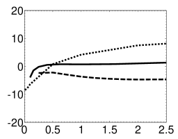
(a) 1-2

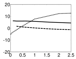
(b) 1-3

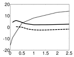
(c) 1-4

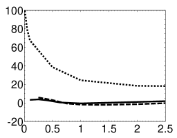
(d) 1-5

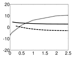
(e) 2-3

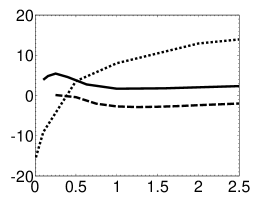
(f) 2-4

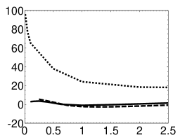
(g) 2-5

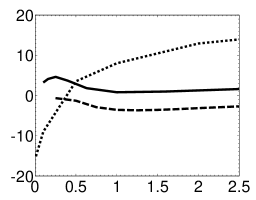
(h) 3-4

(i) 3-5

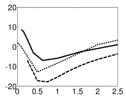
(j) 4-5

Figure 4: Percentage differences of thermally averaged collision strengths from our 72-term Breit-Pauli calculation, (vertical axis) versus temperature in 10000 K (horizontal axis). Results from Lennon & Burke (1994) (solid line), Aggarwal & Keenan (1999) (dashed line) and Palay et al (2012) (dotted line). The labels of the sub-figures refer to the level indices in Table 5.

Figure 5: The difference in derived electron temperature from the $\lambda$4363/($\lambda$4959+$\lambda$5007) line intensity ratio using the data of Lennon & Burke (1994) (solid line), Aggarwal & Keenan (1999) (dashed line) and Palay et al (2012) (dotted line) against the temperature derived from the present results.

Figure 6: Effective collision strength (Upsilon) versus temperature from 72-term target: ICFT with spin-orbit interactions in the target (solid line) and ICFT in pair coupling (dashed line) for the transition between levels 2 and 3 of Table 5.

Figure 7: Percent difference in $\Upsilon$ versus logarithm of temperature between the results of Palay et al (2012) and our 72-term Breit-Pauli calculation for the transitions ³P${}^{\rm{e}}_{{}_{0}}$-¹S${}^{\rm{e}}_{{}_{0}}$ (triangle), ³P${}^{\rm{e}}_{{}_{1}}$-¹S${}^{\rm{e}}_{{}_{0}}$ (circle) and ³P${}^{\rm{e}}_{{}_{2}}$-¹S${}^{\rm{e}}_{{}_{0}}$ (square).

4 Conclusions

In the present paper, the collision strengths for the transitions between the lowest five levels of the astronomically-important ${\rm O}^{2+}+e^{-}$ atomic system up to about 1.3 Rydberg of electron excitation energy are computed in the close coupling approximation using the UCL-Belfast-Strathclyde R-matrix atomic code. Different coupling schemes with different atomic definitions and parameters are used to describe the scattering target and scattering process.

Our results were extensively compared to previous work. We found a good agreement in most cases which increases our confidence in our results. However, we found significant differences with Palay et al (2012) who also used a Breit-Pauli coupling scheme and hence a better agreement was expected. The good agreement between our R-matrix Breit-Pauli calculation and earlier R-matrix work in which the fine-structure was treated more approximately strongly supports our results. We showed that the relatively large differences found for the excitation of the $\lambda 4363$ line between the work of Palay et al (2012) on the one hand, and all previous calculations, on the other, leads to significant differences in derived temperatures from the main [O iii] line ratios.

With regard to the use of the ICFT method, for lowly ionized systems some resonances can have very low principal quantum number, and channels are deeply closed, which can cause problems for multichannel quantum defect theory. This difficulty can be overcome by explicitly omitting channels with very low effective quantum number and in any case evaporates as the effective charge number increases.

5 Acknowledgments and Statement

The work of PJS and NRB was supported in part by STFC (grant ST/J000892/1). Full-precision data for the energy-dependent collision strengths of the transitions between the lowest five levels of the investigated ${\rm O}^{2+}+e^{-}$ system using the 72-term target under a Breit-Pauli intermediate coupling scheme can be obtained in electronic format from the Centre de Données astronomiques de Strasbourg database.

Table 7: Comparison of thermally averaged collision strengths, $\Upsilon$, from Lennon & Burke (1994) (LB) and the current work within the lowest five levels as a function of temperature. The first row of each temperature is from Table 3 of LB and the second row is from the current work using the Breit-Pauli 72-term target.

log $T$ [K]	3P${}^{\rm{e}}_{{}_{0}}$-3P${}^{\rm{e}}_{{}_{1}}$	3P${}^{\rm{e}}_{{}_{0}}$-3P${}^{\rm{e}}_{{}_{2}}$	3P${}^{\rm{e}}_{{}_{1}}$-3P${}^{\rm{e}}_{{}_{2}}$	3Pe-1D${}^{\rm{e}}_{{}_{2}}$	3Pe-1S${}^{\rm{e}}_{{}_{0}}$	1D${}^{\rm{e}}_{{}_{2}}$-1S${}^{\rm{e}}_{{}_{0}}$
3.0	0.4975	0.2455	1.1730	2.2233	0.2754	0.4241
	0.5199	0.2313	1.1218	2.1331	0.2667	0.3897
3.2	0.5066	0.2493	1.1930	2.1888	0.2738	0.4268
	0.5154	0.2349	1.1430	2.0811	0.2643	0.3968
3.4	0.5115	0.2509	1.2030	2.1416	0.2713	0.4357
	0.5132	0.2367	1.1558	2.0237	0.2610	0.4200
3.6	0.5180	0.2541	1.2180	2.1117	0.2693	0.4652
	0.5158	0.2398	1.1736	2.0107	0.2616	0.4799
3.8	0.5296	0.2609	1.2480	2.1578	0.2747	0.5232
	0.5260	0.2462	1.2057	2.0913	0.2732	0.5621
4.0	0.5454	0.2713	1.2910	2.2892	0.2925	0.5815
	0.5421	0.2568	1.2526	2.2425	0.2941	0.6174
4.2	0.5590	0.2832	1.3350	2.4497	0.3174	0.6100
	0.5551	0.2698	1.2994	2.3987	0.3165	0.6254
4.4	0.5678	0.2955	1.3730	2.5851	0.3405	0.6090
	0.5609	0.2835	1.3378	2.5184	0.3339	0.6022

Table 8: Comparison of thermally averaged collision strengths, $\Upsilon$, between Aggarwal (1983) (A), Lennon & Burke (1994) (LB), Aggarwal & Keenan (1999) (AK), Palay et al (2012) (P), and the current work (SSB) using the 72-term target as a function of temperature [K]. The transitions are indexed as in Table 5. Note that the values attributed to Lennon & Burke (1994) for $T=2500$K and $25000$K are those tabulated for log $T=3.4$, $4.4$ in that work.

Index		Temperature [K]
		100	500	1000	2500	5000	7500	10000	12500	15000	17500	20000	25000	30000
1-2	A				0.5041	0.5172	0.5310	0.5417	0.5490	0.5537	0.5567	0.5586	0.5612	0.5633
	LB			0.4975	0.5115			0.5454					0.5678
	AK				0.5011	0.5084	0.5159	0.5222	0.5266	0.5294	0.5311	0.5324	0.5348	0.5380
	P	0.5814	0.5005	0.4866		0.5240		0.5648				0.6007		0.6116
	SSB	0.6350	0.5430	0.5199	0.5132	0.5199	0.5317	0.5421	0.5494	0.5540	0.5569	0.5587	0.5609	0.5623
1-3	A				0.2499	0.2566	0.2646	0.2717	0.2776	0.2824	0.2865	0.2901	0.2962	0.3013
	LB			0.2455	0.2509			0.2713					0.2955
	AK				0.2406	0.2449	0.2512	0.2573	0.2626	0.2669	0.2707	0.2739	0.2798	0.2855
	P	0.2142	0.2153	0.2234		0.2469		0.2766				0.3106		0.3264
	SSB	0.2259	0.2247	0.2313	0.2367	0.2424	0.2497	0.2568	0.2629	0.2682	0.2727	0.2766	0.2833	0.2890
1-4	A				0.2283	0.2262	0.2337	0.2426	0.2506	0.2627	0.2627	0.2672	0.2740	0.2790
	LB			0.2470	0.2380			0.2544					0.2872
	AK				0.2260	0.2265	0.2343	0.2434	0.2515	0.2582	0.2637	0.2683	0.2751	0.2799
	P	0.1959	0.2088	0.2154		0.2347		0.2693				0.3094		0.3256
	SSB	0.2318	0.2389	0.2370	0.2249	0.2265	0.2381	0.2492	0.2579	0.2646	0.2698	0.2739	0.2797	0.2832
1-5	A				0.0278	0.0280	0.0295	0.0310	0.0324	0.0335	0.0344	0.0351	0.0362	0.0368
	LB			0.0306	0.0301			0.0325					0.0378
	AK				0.0307	0.0304	0.0310	0.0321	0.0332	0.0342	0.0351	0.0358	0.0370	0.0378
	P	0.0597	0.0535	0.0496		0.0409		0.0407				0.0430		0.0442
	SSB	0.0299	0.0298	0.0296	0.0290	0.0295	0.0312	0.0327	0.0339	0.0349	0.0357	0.0363	0.0371	0.0375
2-3	A				1.1925	1.2239	1.2592	1.2884	1.3107	1.3275	1.3404	1.3510	1.3679	1.3821
	LB			1.1730	1.2030			1.2910					1.3730
	AK				1.1680	1.1870	1.2100	1.2320	1.2490	1.2620	1.2730	1.2820	1.2980	1.3150
	P	1.0360	1.0320	1.0720		1.2100		1.3300				1.4510		1.4990
	SSB	1.1121	1.0928	1.1218	1.1557	1.1873	1.2221	1.2526	1.2763	1.2943	1.3082	1.3194	1.3374	1.3518
2-4	A				0.6848	0.6785	0.7010	0.7279	0.7518	0.7716	0.7879	0.8014	0.8221	0.8368
	LB			0.7411	0.7139			0.7631					0.8617
	AK				0.6780	0.6795	0.7029	0.7302	0.7545	0.7746	0.7911	0.8049	0.8253	0.8397
	P	0.5903	0.6285	0.6483		0.7067		0.8108				0.9313		0.9802
	SSB	0.6975	0.7187	0.7132	0.6772	0.6823	0.7175	0.7506	0.7768	0.7969	0.8125	0.8247	0.8421	0.8527
2-5	A				0.0833	0.0840	0.0884	0.0931	0.0972	0.1006	0.1033	0.1054	0.1085	0.1105
	LB			0.0918	0.0904			0.0975					0.1135
	AK				0.0921	0.0911	0.0929	0.0962	0.0995	0.1025	0.1052	0.1074	0.1109	0.1135
	P	0.1765	0.1590	0.1477		0.1228		0.1223				0.1294		0.1332
	SSB	0.0900	0.0897	0.0892	0.0873	0.0890	0.0939	0.0985	0.1022	0.1052	0.1075	0.1093	0.1118	0.1131
3-4	A				1.1413	1.1308	1.1683	1.2131	1.2529	1.2860	1.3132	1.3357	1.3702	1.3947
	LB			1.2352	1.1898			1.2718					1.4362
	AK				1.1300	1.1325	1.1715	1.2170	1.2575	1.2910	1.3185	1.3415	1.3755	1.3995
	P	0.9934	1.0560	1.0890		1.1880		1.3630				1.5640		1.6450
	SSB	1.1702	1.2057	1.1965	1.1374	1.1474	1.2066	1.2620	1.3055	1.3389	1.3647	1.3850	1.4137	1.4310
3-5	A				0.1388	0.1401	0.1473	0.1552	0.1620	0.1676	0.1721	0.1757	0.1809	0.1842
	LB			0.1530	0.1507			0.1625					0.1892
	AK				0.1536	0.1518	0.1549	0.1603	0.1659	0.1709	0.1753	0.1790	0.1849	0.1891
	P	0.2850	0.2587	0.2421		0.2045		0.2046				0.2170		0.2235
	SSB	0.1512	0.1506	0.1497	0.1467	0.1496	0.1579	0.1657	0.1720	0.1769	0.1808	0.1839	0.1881	0.1902
4-5	A				0.4708	0.5463	0.6114	0.6468	0.6630	0.6687	0.6692	0.6670	0.6599	0.6524
	LB			0.4241	0.4357			0.5815					0.6090
	AK				0.3907	0.4312	0.4836	0.5227	0.5478	0.5629	0.5719	0.5769	0.5809	0.5812
	P	0.3900	0.3899	0.3899		0.4544		0.5661				0.6230		0.6219
	SSB	0.3827	0.3856	0.3897	0.4196	0.5208	0.5882	0.6174	0.6266	0.6265	0.6223	0.6163	0.6026	0.5886

References

- Aggarwal (1983) Aggarwal K.M., 1983, ApJS, 52, 387
- Aggarwal (1985) Aggarwal K.M., 1985, A&A, 146, 149
- Aggarwal (1993) Aggarwal K.M., 1993, ApJS, 85, 197
- Aggarwal & Hibbert (1991) Aggarwal K.M., Hibbert A., 1991, J. Phys. B, 24, 3445
- Aggarwal & Keenan (1999) Aggarwal K.M., Keenan F.P., 1999, ApJS, 123, 311
- Badnell (2011) Badnell N.R., 2011, Comput. Phys. Commun., 182, 1528
- Baluja et al (1980) Baluja K.L., Burke P.G., Kingston A.E., 1980, J. Phys. B, 13, 829
- Berrington et al (1974) Berrington K.A., Burke P.G., Chang J.J., Chivers A.T., Robb W.D., Taylor K.T., 1974, Comp. Phys. Comm., 8, 149
- Berrington et al (1987) Berrington K.A., Burke P.G., Butler K., Seaton M.J., Storey P.J., Taylor K.T., Yu Yan., 1987, J. Phys. B, 20, 6379
- Berrington et al (1995) Berrington K.A., Eissner W.B., Norrington P.H., 1995, Comp. Phys. Comm., 92, 290
- Bhatia et al (1979) Bhatia A.K., Doschek G.A., Feldman U., 1979, A&A, 76, 359
- Bohm & Aller (1947) Bohm D., Aller L.H., 1947, ApJ, 105, 131
- Czyzak et al (1968) Czyzak S.J., Krueger T.K., de Martins P.A.P., Saraph H.E., Seaton M.J., Shemming J., 1968, In Planetary Nebulae by Osterbrock D.E. and O’Dell C.R. (Editors), 34, 138
- Eissner et al (1974) Eissner W., Jones M., Nussbaumer H., 1974, Comp. Phys. Comm., 8, 270
- Gorczyca & Badnell (2000) Gorczyca T.W., Badnell N.R. 2000, J. Phys. B, 33, 2955
- Griffin, Badnell & Pindzola (1998) Griffin D.C., Badnell N.R., Pindzola M.S., 1998, J. Phys. B, 31, 3713
- Hagihara (1944) Hagihara Y., 1944, Proceedings of the Japan Academy, 20, 493
- Ho & Henry (1983) Ho Y.K., Henry R.J.W., 1983, ApJ, 264, 733
- Hibbert (1975) Hibbert A., 1975, Comp. Phys. Comm., 9, 141
- Hummer et al (1993) Hummer D.G., Berrington K.A., Eissner W., Pradhan A.K., Saraph H.E., Tully J.A., 1993, A&A, 279, 298
- Lennon & Burke (1994) Lennon D.J., Burke V.M., 1994, A&AS, 103, 273
- Burke, Lennon & Seaton (1989) Burke V.M., Lennon, D.J., Seaton, M.J., 1989, MNRAS, 236, 353
- Maiolino et al (2008) Maiolino R., Nagao T., Grazian A., et al, 2008, A&A, 488, 463
- Nicholls et al (2012) Nicholls D.C., Dopita M.A., Sutherland R.S., 2012, ApJ, 752, 148
- Nussbaumer & Storey (1978) Nussbaumer H., Storey P.J., 1978, A&A, 64, 139
- Nussbaumer & Storey (1981) Nussbaumer H., Storey P.J., 1981, A&A, 99, 177
- Palay et al (2012) Palay E., Nahar S.N., Pradhan A.K., Eissner W., 2012, MNRAS Let., 423, L35
- Saraph (1978) Saraph, H.E., 1978, Comp. Phys. Comm., 15, 247
- Seaton (1975) Seaton M.J., 1975, MNRAS, 170, 475
- Sochi (2012) Sochi T., 2012, PhD thesis, University College London
- Sochi & Storey (2013) Sochi T., Storey P.J., 2013, ADNDT, 99, 633
- Storey & Sochi (2013) Storey P.J., Sochi T., 2013, MNRAS, 430, 599
- Storey & Zeippen (2000) Storey P.J., Zeippen C.J., 2000, MNRAS 312, 813
- Vasyliunas (1968) Vasyliunas V.M., 1968, JGR, 73, 2839