The Yield Condition in the Mobilization of Yield-Stress Materials in Distensible Tubes

Abstract

In this paper we investigate the yield condition in the mobilization of yield-stress materials in distensible tubes. We discuss the two possibilities for modeling the yield-stress materials prior to yield: solid-like materials and highly-viscous fluids and identify the logical consequences of these two approaches on the yield condition. As part of this investigation we derive an analytical expression for the pressure field inside a distensible tube with a Newtonian flow using a one-dimensional Navier-Stokes flow model in conjunction with a pressure-area constitutive relation based on elastic tube wall characteristics.

Keywords: fluid mechanics; yield-stress; yield condition; distensible tube; pressure field.

1 Introduction

Many naturally-occurring and synthetic materials are characterized by being yield-stress fluids, that is they behave like solids under low shear stresses and as fluids on exceeding a minimum threshold yield-stress [1, 2, 3, 4, 5]. Blood and crude oils are some examples of naturally-occurring yield-stress fluids while many manufactured products used in the food and petrochemical industries; like purees, yoghurts, slurries, drilling muds, and polymeric solutions; are examples of synthetic yield-stress materials [6, 7, 8, 9, 10, 3, 11, 12, 13, 14, 15, 16, 17, 18, 19, 20]. As these materials can reside and mobilize in rigid conduits and structures, such as oil transportation pipelines and geological porous formations, they can also reside and mobilize in compliant conduits and structures like blood vessels and living porous tissues. Hence the investigation of the circumstances and conditions under which these materials yield and start flowing in rigid and distensible containers is important for modeling and analyzing many industrial and natural flow systems.

We are not aware of a previous attempt to find the condition for the yield of yield-stress materials in distensible tubes. Past investigations are generally focused on the flow of yield-stress fluids in rigid conduits and structures such as ensembles of conduits and porous media [21, 22, 23, 24, 25, 4, 26, 27, 28, 29]. There are some other studies (e.g. [30]) that investigated the flow of yield-stress fluids in distensible conduits but the focus of these studies is not on the yield condition but on the flow of these materials assuming they have already reached a fluid phase state by satisfying the mobilization condition.

To clarify the purpose of the current investigation, we define the yield condition in general terms that include rigid and distensible flow conduits as the minimum pressure drop across the conduit that mobilizes the yield-stress material and forces it to flow following an initial solid state condition. The yield point is therefore reached through increasing the pressure drop applied on the material in its solid state gradually or suddenly. This definition is also valid in principle for the yield condition in the bulk flow although this is not of interest to us in the current investigation.

In the present paper we investigate the yield condition in the mobilization of yield-stress materials through distensible tubes using an elastic model for the tube wall that correlates the pressure at a given axial coordinate to the corresponding cross sectional area. Although we assume a circular cylindrical tube with a constant unstressed radius over its length, some of the presented arguments at least can be generalized to include other cases although we are not intending to do so in the current study.

In this investigation, we are only concerned with the yield condition as it is, without interest in other issues related to the flow of yield-stress fluids in these conduits; hence any other dynamic issues associated with the flow phase are out of scope of the present paper. Our plan for the paper is to introduce the one-dimensional Navier-Stokes flow model which is widely used to describe the flow of Newtonian fluids in distensible tubes. The reason for using this model, which is a Newtonian model and not a yield-stress model, is that prior to yield the yield-stress materials according to one approach behave as highly-viscous Newtonian fluids. We also discuss the pressure field inside the tube under such a Navier-Stokes flow condition and how this field can be computed analytically and numerically because it is needed for identifying the yield condition. This will be followed by a section in which we investigate the yield condition in detail considering two approaches for modeling the yield-stress materials prior to yield. A general assessment of our proposed method for identifying the yield condition with some synopsis conclusions will then follow.

2 One-Dimensional Navier-Stokes Model

The flow of Newtonian fluids in a circular cylindrical tube with length $L$ and cross sectional area $A$ assuming an incompressible laminar axi-symmetric flow with a negligible gravitational force is described by the following one-dimensional Navier-Stokes system of mass and momentum conservation principles

$$\frac{\partial A}{\partial t}+\frac{\partial Q}{\partial x} = 0\,\,\,\,\,\,\,\,\,\,\,\,\,t\geq 0,\,\,\,x\in[0,L]$$ (1)

$$\frac{\partial Q}{\partial t}+\frac{\partial}{\partial x}\left(\frac{\alpha Q^{2}}{A}\right)+\frac{A}{\rho}\frac{\partial p}{\partial x}+\kappa\frac{Q}{A} = 0\,\,\,\,\,\,\,\,\,\,\,\,\,t\geq 0,\,\,\,x\in[0,L]$$ (2)

where $Q$ is the volume flow rate, $x$ is the tube axial coordinate along its length, $t$ is the elapsed time for the flow process, $\rho$ is the fluid mass density, $\alpha$ is the correction factor for the momentum flux, $p$ is the axial pressure along the tube length which is a function of the axial coordinate, and $\kappa$ is a viscosity friction coefficient which is normally defined by $\kappa=\frac{2\pi\alpha\mu}{\rho(\alpha-1)}$ where $\mu$ is the fluid dynamic viscosity [31, 32, 33, 34]. In this context we assume a no-slip at wall condition where the velocity of the fluid at the interface is identical to the velocity of the solid [35, 36, 37]. This Navier-Stokes system is normally supported by a constitutive relation that links the cross sectional area at a certain axial location to the corresponding axial pressure in a distensible tube, to close the system in the three variables $Q$, $A$ and $p$ and hence provide a complete mathematical description for such a flow in such a conduit.

The relation between the cross sectional area and the axial pressure in a distensible tube can be described by many mathematical models depending on the characteristics of the tube wall and its mechanical response to pressure such as being linear or non-linear, and elastic or viscoelastic. The following is an example of a commonly used pressure-area constitutive elastic relation that describes such a dependency

$$p=\frac{\beta}{A_{o}}\left(\sqrt{A}-\sqrt{A_{o}}\right)$$ (3)

where $A_{o}$ is the reference cross sectional area corresponding to the reference pressure which in this equation is set to zero for convenience without affecting the generality of the results, $A$ is the tube cross sectional area corresponding to the axial pressure $p$ as opposite to the reference pressure, and $\beta$ is the tube wall stiffness coefficient which is usually defined by

$$\beta=\frac{\sqrt{\pi}h_{o}E}{1-\varsigma^{2}}$$ (4)

where $h_{o}$ is the tube wall thickness at the reference pressure, while $E$ and $\varsigma$ are respectively the Young’s elastic modulus and Poisson’s ratio of the tube wall. In this context, we assume a constant ambient pressure surrounding the tube that is set to zero and hence the reference cross sectional area represents unstressed state with $A_{o}$ being constant over the axial coordinate.

Now, to find the axial pressure field inside an elastic tube characterized by the mechanical response of Equation 3 we combine the pressure-area constitutive relation with the mass and momentum equations of Navier-Stokes system. In the following we assume a pressure drop applied on the tube by imposing two boundary conditions at $x=0$ and $x=L$ and hence it is identified by two pressure boundary conditions, $p_{in}$ and $p_{ou}$, where

$$p_{in}\equiv p\left(x=0\right)>p_{ou}\equiv p\left(x=L\right)$$ (5)

Another clarifying remark is that for a sustainable flow in a distensible tube, the tube axial pressure should be a monotonically decreasing function of its axial coordinate. As a result, the radius and the cross sectional area of the tube are also monotonically decreasing functions of the axial coordinate. This fact is assumed in most of the following arguments although it may not be stated explicitly.

From the pressure-area constitutive relation we have

$$p=\frac{\beta}{A_{o}}\left(\sqrt{A}-\sqrt{A_{o}}\right)$$ (6)

and hence

$$A=\left(\frac{A_{o}}{\beta}p+\sqrt{A_{o}}\right)^{2}$$ (7)

and

$$\frac{\partial A}{\partial p}=2\frac{A_{o}}{\beta}\left(\frac{A_{o}}{\beta}p+\sqrt{A_{o}}\right)=\frac{2A_{o}^{2}}{\beta^{2}}p+\frac{2A_{o}^{3/2}}{\beta}$$ (8)

For a steady state flow the time terms in the Navier-Stokes system are zero and hence from the continuity equation (Equation 1) $Q$ as a function of $x$ is constant. Consequently, from the momentum equation of the Navier-Stokes system (Equation 2) we obtain

$$\frac{\partial}{\partial x}\left(\frac{\alpha Q^{2}}{A}\right)+\frac{A}{\rho}\frac{\partial p}{\partial x}+\kappa\frac{Q}{A}=0$$ (9)

which can be manipulated to obtain the axial pressure gradient as follow

$$\alpha Q^{2}\frac{\partial}{\partial A}\left(\frac{1}{A}\right)\frac{\partial A}{\partial p}\frac{\partial p}{\partial x}+\frac{A}{\rho}\frac{\partial p}{\partial x}+\kappa\frac{Q}{A}=0$$ (10)

$$-\frac{\alpha Q^{2}}{A^{2}}\frac{\partial A}{\partial p}\frac{\partial p}{\partial x}+\frac{A}{\rho}\frac{\partial p}{\partial x}+\kappa\frac{Q}{A}=0$$ (11)

$$-\frac{\alpha Q^{2}}{A^{2}}\left(\frac{2A_{o}^{2}}{\beta^{2}}p+\frac{2A_{o}^{3/2}}{\beta}\right)\frac{\partial p}{\partial x}+\frac{A}{\rho}\frac{\partial p}{\partial x}+\kappa\frac{Q}{A}=0$$ (12)

$$\frac{\partial p}{\partial x}\left[-\frac{\alpha Q^{2}}{A^{2}}\left(\frac{2A_{o}^{2}}{\beta^{2}}p+\frac{2A_{o}^{3/2}}{\beta}\right)+\frac{A}{\rho}\right]=-\kappa\frac{Q}{A}$$ (13)

that is

$$\frac{\partial p}{\partial x}=\frac{\kappa\frac{Q}{A}}{\frac{\alpha Q^{2}}{A^{2}}\left(\frac{2A_{o}^{2}}{\beta^{2}}p+\frac{2A_{o}^{3/2}}{\beta}\right)-\frac{A}{\rho}}$$ (14)

The last expression can be simplified to

$$\frac{\partial p}{\partial x}=\frac{\kappa Q\left(\frac{A_{o}}{\beta}p+\sqrt{A_{o}}\right)^{2}}{\alpha Q^{2}\left(\frac{2A_{o}^{2}}{\beta^{2}}p+\frac{2A_{o}^{3/2}}{\beta}\right)-\frac{\left(\frac{A_{o}}{\beta}p+\sqrt{A_{o}}\right)^{6}}{\rho}}$$ (15)

which expresses the axial pressure gradient, $\frac{\partial p}{\partial x}$, as a function of the tube axial pressure, $p$, only. For a one-dimensional steady state flow, the pressure is dependent on the tube axial coordinate only and hence the partial derivative of Equation 15 can be replaced with a total derivative. On separating the variables and carrying out the integration, where $0\leq x\leq L$ and $p_{ou}\leq p\leq p_{in}$, we obtain

$$x=\frac{2\alpha Q\ln\left(\frac{A_{o}}{\beta}p+\sqrt{A_{o}}\right)}{\kappa}-\frac{\beta\left(\frac{A_{o}}{\beta}p+\sqrt{A_{o}}\right)^{5}}{5\rho\kappa QA_{o}}+C$$ (16)

where $C$ is the constant of integration which can be determined from the boundary conditions. At $x=0$ $p=p_{in}$, and hence

$$C=-\frac{2\alpha Q\ln\left(\frac{A_{o}}{\beta}p_{in}+\sqrt{A_{o}}\right)}{\kappa}+\frac{\beta\left(\frac{A_{o}}{\beta}p_{in}+\sqrt{A_{o}}\right)^{5}}{5\rho\kappa QA_{o}}$$ (17)

The analytical solution of the pressure field, as given by Equation 16, defines the axial pressure field $p(x)$ as an implicit function of the axial coordinate $x$. Obtaining the pressure field then requires either the employment of a simple numerical solver, based for example on a bisection method, or changing the role of the independent and dependent variables and hence obtaining $x$ as a function of $p$ where the value of pressure is constrained by the two boundary conditions. The latter scheme, which is more convenient to use, leads to the same result as the first scheme although the defining $x$-$p$ points are determined by the pressure points and hence obtaining a smoothly defined pressure field may require computing more points than is needed from the first scheme. In addition to the convenience, the solution obtained from the second scheme is generally more accurate because it produces exact solutions within the available computing precision although this extra accuracy may be of little value in practical circumstances.

The analytical solution of Equation 16 was tested and validated by numerical solutions from many typical flow examples using the lubrication approximation with a residual-based Newton-Raphson solution scheme. This numerical method for obtaining the pressure field and flow rate is based on discretizing the flow conduit into thin rings which are treated as an ensemble of serially connected tubes over which a mass conserving characteristic flow (in this case the one-dimensional Navier-Stokes flow in elastic cylindrical tubes) is sought by forming a system of simultaneous equations derived from the boundary conditions for the boundary nodes and the continuity of volumetric flow rate for the internal nodes. This system is then solved numerically by an iterative non-linear solution scheme, such as Newton-Raphson method, to obtain the axial pressure field inside the conduit, defined at the boundary and internal nodes, as well as the mass-conserving flow rate within a given error tolerance. This numerical solving scheme for obtaining the pressure field and flow rate is fully described in [38, 39, 40]. A sample of the results comparing the analytical to the numerical solutions for some typical examples with a range of tube, flow and fluid parameters are given in Figure 1.

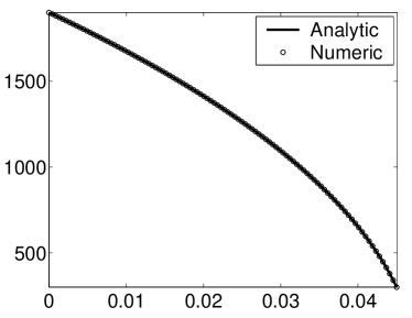
Figure 1: Comparing the analytical solution of the axial pressure field as given by Equation 16 to the numerical solution from the residual-based lubrication approximation for the Navier-Stokes flow in elastic tubes with (a) $R=0.01$, $L=0.1$, $\alpha=\frac{4}{3}$, $\beta=39.5$, $\rho=900$, $\mu=0.01$, $p_{in}=2000$, $p_{ou}=0$, and $Q=2.36708\times 10^{-3}$, (b) $R=0.05$, $L=0.75$, $\alpha=1.25$, $\beta=88.9$, $\rho=1300$, $\mu=0.025$, $p_{in}=2500$, $p_{ou}=500$, and $Q=7.34585\times 10^{-2}$, (c) $R=0.003$, $L=0.045$, $\alpha=1.5$, $\beta=12.9$, $\rho=1100$, $\mu=0.015$, $p_{in}=1900$, $p_{ou}=300$, and $Q=4.66119\times 10^{-5}$, and (d) $R=0.1$, $L=0.9$, $\alpha=1.3$, $\beta=227.7$, $\rho=800$, $\mu=0.035$, $p_{in}=3100$, $p_{ou}=600$, and $Q=2.49237\times 10^{-1}$. All the dimensional quantities are in standard SI units. In all four sub-figures, the vertical axis represents the tube axial pressure in pascals while the horizontal axis represents the tube axial coordinate in meters.

3 Yield Condition

A general definition has been given earlier for the yield condition. However, since the pressure field inside a distensible tube and the resulting flow rate are dependent on the actual value of the two boundary conditions and not only on their difference (i.e. pressure drop) [41] we define the yield condition for distensible tubes as the minimum inlet pressure for a given outlet pressure that mobilizes the yield-stress material and initiates a measurable flow. The generally accepted condition for the yield of a yield-stress material in a tube is given by equating the magnitude of the wall shear stress $|\tau_{w}|$ to the yield-stress of the fluid $\tau_{o}$ where $\tau_{w}$ is defined as the ratio of the force normal to the tube axis $F_{\perp}$ to the area of the luminal surface parallel to this force $A_{\parallel}$.

Our proposal for the condition that should be satisfied to reach the yield point is that yield occurs iff all cross sectional points in the tube along its length reached their yield condition simultaneously. This will only occur if the bottleneck in the tube reaches its yield condition where the bottleneck is the location along the tube axis with the lowest magnitude of wall shear stress. It is obvious that this is a necessary and sufficient condition for yield to occur because if the bottleneck reached its yield condition with its wall shear stress just exceeding the yield-stress then all other points along the tube axis should also satisfy the yield condition.

For a rigid tube with a constant radius along its axial direction, $\tau_{w}$ is given by

$$\tau_{w}\equiv\frac{F_{\perp}}{A_{\parallel}}=\frac{\pi R^{2}\Delta P}{2\pi RL}=\frac{R\Delta P}{2L}$$ (18)

where $R$ and $L$ are the tube radius and length respectively while $\Delta P$ is the pressure drop across the tube.

For a tube with a variable radius along its axial direction, including a distensible tube subjected to a pressure gradient along its axis, the wall shear stress is a function of the tube axial coordinate $x$ and hence the wall shear stress is defined locally as a function of $x$ by using infinitesimal quantities of pressure drop, $\delta p$, and length, $\delta x$, belonging to a thin cross sectional ring over which the change in radius is negligible, that is

$$\tau_{w}\left(x\right)\equiv\frac{F_{\perp}}{A_{\parallel}}\simeq\frac{\pi R^{2}\delta p}{2\pi R\delta x}=\frac{R}{2}\frac{\delta p}{\delta x}$$ (19)

which in the limit becomes

$$\tau_{w}\left(x\right)=\frac{R}{2}\frac{dp}{dx}$$ (20)

Therefore the condition for the transition from the solid state to fluid phase, corresponding to the yield and flow initiation, is defined by the following condition

$$|\tau_{w}|=\tau_{o}\,\,\,\,\,\,\,\,\,\Rightarrow\,\,\,\,\,\,\,\,\,\frac{R(x)}{2}\left|\frac{dp}{dx}\right|=\tau_{o}$$ (21)

There are two possibilities for modeling the yield-stress materials before reaching their yield point: either they are solid-like materials or they are highly-viscous fluids. A detailed discussion about this issue, among other relevant issues, is given in [29]. Our proposal for identifying the yield point according to each one of these two possibilities is discussed in the following two subsections.

3.1 Solid-Like Materials

According to this approach, the yield-stress materials before reaching their yield point behave like solids. Hence, a logical assumption about the pressure field configuration inside the tube prior to mobilization is to assume a linear pressure drop and hence a constant pressure gradient. In this case the bottleneck occurs at the outlet boundary point because the radius of the tube is monotonically decreasing and hence the outlet point is the one with the smallest radius which implies that the wall shear stress as given by Equation 21 is the lowest since $\frac{dp}{dx}$ is assumed constant along the tube axis. Therefore the yield condition according to the solid-like modeling approach is given by

$$\frac{R(L)}{2}\left|\frac{dp}{dx}\right|=\tau_{o}$$ (22)

where $R(L)$ is the tube radius at the outlet boundary corresponding to $x=L$.

3.2 Highly-Viscous Fluids

According to this approach, the yield-stress materials before reaching their yield point are highly-viscous fluids and hence they flow but with an infinitesimally small flow rate. Our proposal in this case is that the material prior to yield should be modeled as a Newtonian fluid with a very high viscosity. The assumption of a Newtonian fluid is justified by the fact that at such regimes of very low rate of deformation the material is at its low Newtonian plateau since all non-Newtonian rheological effects are induced only by a measurable deformation [29]. We therefore use the one-dimensional Navier-Stokes flow model to identify the pressure field prior to yield and hence the yield condition. This one-dimensional Navier-Stokes flow model is fully described in [32, 33]. It is also outlined in section 2 with a derivation of an analytical expression for the axial pressure as an implicit function of the tube axial coordinate. The determination of the axial pressure field is obviously needed for the identification of the yield condition because both $R$ and $\frac{dp}{dx}$ are dependent on the pressure field.

Our general approach for identifying the yield condition assuming a highly-viscous fluid prior to yield is to test the axial pressure field as determined by the given inlet and outlet boundary conditions. The purpose of this test is to identify the bottleneck by determining the lowest wall shear stress in magnitude along the tube and hence verifying if the bottleneck has reached its minimum threshold which equals the yield-stress value, $\tau_{o}$. As seen in Equation 21, $|\tau_{w}|$ is dependent on the pressure gradient and the tube radius as functions of the axial coordinate. Hence a knowledge of these two quantities is required.

There are two ways for obtaining the pressure gradient and the tube radius. The first way is to solve the pressure field numerically using the aforementioned residual-based lubrication approach. The axial pressure gradient is then calculated from the numerical solution of the pressure field either analytically from Equation 15 or numerically using for instance a finite difference method. On knowing the axial pressure, the tube radius as a function of the axial coordinate can also be computed from the pressure-area constitutive relation (Equation 7). The second way is to use the analytical solution of the pressure field, which is derived in section 2, and hence evaluate the axial pressure gradient and axial radius as in the case of numerical solution of the pressure field, although the analytical evaluation of the pressure gradient from Equation 15 may not be possible unless $Q$ is obtained from another method. Both of these ways practically produce the same result if a sufficiently fine mesh is used for discretizing the tube in the residual-based lubrication technique.

As indicated early, in the case of using the analytical expression of Equation 16 a simple numeric solver, based for instance on a bisection method, can be used to evaluate the axial pressure which is given as an implicit function of the tube axial coordinate. An alternative and more convenient way that does not require the employment of a numerical solver is to use Equation 16 to find the axial coordinate $x$ as a function of the axial pressure $p$, which is as good for evaluating the axial pressure field as the other way round. The use of one of these methods or the other (i.e. numerical or analytical with or without the employment of a numerical solver) is a matter of choice and convenience. All our numerical experiments produced essentially the same results on using these different methods and techniques.

However, it can be shown that the bottleneck, according to the highly-viscous fluid approach, is always at the inlet boundary and hence the use of the numerical and analytical methods is unnecessary apart from providing the one-sided pressure gradient at the inlet since the inlet radius is already known from the inlet boundary condition. The justification of this is explained in the following paragraphs.

As stated before, for a steady state flow the time terms in the Navier-Stokes system are zero and hence from the continuity equation (Equation 1) $Q$ as a function of $x$ is constant. Hence, from the momentum equation of the Navier-Stokes system (Equation 2) we obtain

$$\frac{\partial}{\partial x}\left(\frac{\alpha Q^{2}}{A}\right)+\frac{A}{\rho}\frac{\partial p}{\partial x}+\kappa\frac{Q}{A}=0$$ (23)

$$\frac{\partial p}{\partial x}=-\frac{\rho}{A}\left[\kappa\frac{Q}{A}+\frac{\partial}{\partial x}\left(\frac{\alpha Q^{2}}{A}\right)\right]$$ (24)

$$\frac{\partial p}{\partial x}=-\left(\frac{\kappa\rho Q}{A^{2}}+\frac{\rho\alpha Q^{2}}{A}\frac{\partial A^{-1}}{\partial x}\right)$$ (25)

$$\frac{\partial p}{\partial x}=-\left(\frac{\kappa\rho Q}{A^{2}}+\frac{\rho\alpha Q^{2}}{A}\frac{\partial A^{-1}}{\partial A}\frac{\partial A}{\partial x}\right)$$ (26)

that is

$$\frac{\partial p}{\partial x}=-\left(\frac{\kappa\rho Q}{A^{2}}-\frac{\rho\alpha Q^{2}}{A^{3}}\frac{\partial A}{\partial x}\right)$$ (27)

Now since $A$ is a monotonically decreasing function of $x$

$$-\frac{\partial A}{\partial x}=\left|\frac{\partial A}{\partial x}\right|$$ (28)

and hence

$$\frac{\partial p}{\partial x}=-\left(\frac{\kappa\rho Q}{A^{2}}+\frac{\rho\alpha Q^{2}}{A^{3}}\left|\frac{\partial A}{\partial x}\right|\right)$$ (29)

Therefore

$$|\tau_{w}|=\frac{R}{2}\left|\frac{\partial p}{\partial x}\right|=\frac{R}{2}\left(\frac{\kappa\rho Q}{\pi^{2}R^{4}}+\frac{\rho\alpha Q^{2}}{\pi^{3}R^{6}}\left|\frac{\partial A}{\partial x}\right|\right)$$ (30)

$$|\tau_{w}|=\left(\frac{\kappa\rho Q}{2\pi^{2}R^{3}}+\frac{\rho\alpha Q^{2}}{2\pi^{3}R^{5}}\frac{\partial A}{\partial R}\left|\frac{\partial R}{\partial x}\right|\right)$$ (31)

$$|\tau_{w}|=\left(\frac{\kappa\rho Q}{2\pi^{2}R^{3}}+\frac{\rho\alpha Q^{2}}{2\pi^{3}R^{5}}2\pi R\left|\frac{\partial R}{\partial x}\right|\right)$$ (32)

$$|\tau_{w}|=\left(\frac{\kappa\rho Q}{2\pi^{2}R^{3}}+\frac{\rho\alpha Q^{2}}{\pi^{2}R^{4}}\left|\frac{\partial R}{\partial x}\right|\right)$$ (33)

that is

$$|\tau_{w}|=\frac{B}{R^{3}}+\frac{C}{R^{4}}\left|\frac{\partial R}{\partial x}\right|$$ (34)

where

$$B=\frac{\kappa\rho Q}{2\pi^{2}}>0\,\,\,\,\,\,\,\,\,\,\ \textrm{and}\,\,\,\,\,\,\,\,\,\,\,C=\frac{\rho\alpha Q^{2}}{\pi^{2}}>0$$ (35)

In the following we will show that $f\equiv|\tau_{w}|$ is a monotonically increasing function of $x$ by demonstrating that the first derivative of $f$ is positive, i.e. $\frac{\partial f}{\partial x}>0$.

$$\frac{\partial f}{\partial x}=\frac{\partial}{\partial x}\left(\frac{B}{R^{3}}+\frac{C}{R^{4}}\left|\frac{\partial R}{\partial x}\right|\right)$$ (36)

Now, since $R$ is a monotonically decreasing function of $x$ we have

$$\left|\frac{\partial R}{\partial x}\right|=-\frac{\partial R}{\partial x}$$ (37)

and

$$\frac{\partial\left|\frac{\partial R}{\partial x}\right|}{\partial x}=-\frac{\partial^{2}R}{\partial x^{2}}$$ (38)

Therefore

$$\frac{\partial f}{\partial x}=-\frac{3B}{R^{4}}\frac{\partial R}{\partial x}-\frac{4C}{R^{5}}\frac{\partial R}{\partial x}\left|\frac{\partial R}{\partial x}\right|-\frac{C}{R^{4}}\frac{\partial^{2}R}{\partial x^{2}}$$ (39)

$$\frac{\partial f}{\partial x}=\frac{3B}{R^{4}}\left|\frac{\partial R}{\partial x}\right|+\frac{4C}{R^{5}}\left|\frac{\partial R}{\partial x}\right|^{2}-\frac{C}{R^{4}}\frac{\partial^{2}R}{\partial x^{2}}$$ (40)

$$\frac{\partial f}{\partial x}>0\,\,\,\,\Rightarrow\,\,\,\,\frac{C}{R^{4}}\frac{\partial^{2}R}{\partial x^{2}}<\frac{3B}{R^{4}}\left|\frac{\partial R}{\partial x}\right|+\frac{4C}{R^{5}}\left|\frac{\partial R}{\partial x}\right|^{2}$$ (41)

i.e.

$$\frac{\partial^{2}R}{\partial x^{2}}<\frac{3B}{C}\left|\frac{\partial R}{\partial x}\right|+\frac{4}{R}\left|\frac{\partial R}{\partial x}\right|^{2}\,\,\,\,\,\,\,\,\left(R>0\right)$$ (42)

Now, $\frac{\partial^{2}R}{\partial x^{2}}$ is either negative or positive. If it is negative then the condition given by Equation 42 is always satisfied because the right hand side is strictly positive. However, if it is positive then since

$$\frac{B}{C}=\frac{\kappa}{2\alpha Q}$$ (43)

we can show that in all practical situations the first term on the right hand side is greater than the left hand side regardless of the magnitude of the second term on the right hand side. The reason is that prior to yield $Q$ is infinitesimally small, and therefore $\frac{B}{C}$ is very large in magnitude and positive in sign. Hence for any tangible pressure drop that makes $\left|\frac{\partial R}{\partial x}\right|$ finite, which is automatically satisfied for any tangible yield-stress, the first term on the right hand side is very large. Therefore, for all practical purposes where the curvature of the tube, as quantified by the second derivative of $R$ with respect to $x$, is constrained within the physical limits the condition given by Equation 42 will be satisfied. This means that in both cases the first derivative of $f$ is greater than zero and hence the absolute value of the wall shear stress, $|\tau_{w}|$, is a monotonically increasing function of the tube axial coordinate $x$.

As a result, the bottleneck according to the highly-viscous fluid approach will always be at the inlet boundary. This finding is confirmed by numerical experiments where all the results indicate that the bottleneck is at the inlet boundary. It should be remarked that it can be demonstrated that for the one-dimensional Navier-Stokes flow in an elastic tube whose mechanical response is described by Equation 3 it is always the case that $\frac{\partial^{2}R}{\partial x^{2}}<0$, i.e. the axial dependency of the radius, area and pressure concave downward (refer for instance to Figure 1). However, we will not prove this here to avoid unnecessary details because, as demonstrated already, this is not needed for establishing our case.

To sum up, the identification of the bottleneck through the inspection of the axial pressure field by using the numerical or the analytical solution is the generally valid method and hence it should provide a definite and reliable answer for determining the yield condition. However, as demonstrated in the previous paragraphs, at least for all the practical purposes in which the distensible tube is not subjected to extremely large pressure boundary conditions which invalidate the pressure-area relation, the bottleneck and hence the yield condition can be identified from just inspecting the magnitude of the wall shear stress at the inlet boundary, which as explained earlier only requires computing the one-sided pressure gradient numerically or analytically. In all cases, tests can be carried out to verify that the bottleneck is actually at the inlet boundary.

4 General Assessment

The method proposed in this paper for the identification of the yield condition in the mobilization of yield-stress materials in distensible tubes is based on a number of simplifying assumptions regarding the fluid, flow and tube. The purpose of this investigation is to derive the yield condition from logical reasoning through the employment of the principles of mechanics, rheology and fluid dynamics. Many practical factors that usually arise in real life can change this condition and hence require a deeper inspection to identify the yield condition more rigorously. The real yield-stress flow systems are more physically complex than the description provided by our model or any other model since all these models are based on mathematical idealizations and physical simplifications. However, we believe this investigation can provide the ground for further investigations in the future through which more complex factors can be incorporated in the modeled yield-stress flow systems to provide better predictions for the yield condition.

5 Conclusions

The investigation in the present paper lead to the proposal of a method for identifying the yield condition in the mobilization of yield-stress materials through deformable cylindrical tubes with a constant unstressed cross sectional area along their axial length. Two possible scenarios for modeling the yield-stress materials prior to yield have been considered: a solid-like approach and a highly-viscous fluid approach. The logical consequences of these two approaches were derived using the principles of rheology and fluid dynamics as summarized in the rheological characteristics of the deformed material, Navier-Stokes system and the distensibility characteristics of the tube wall. General mechanical principles were also employed in this investigation with regard to the solid-like approach.

Although the derived yield condition is based on several simplifying assumptions with regard to the type of flow, fluid and tube characteristics and hence it applies to a rather idealized yield-stress flow system, the proposed model can serve as a first step for more elaborate yield-stress models that incorporate more physical factors that influence the yield condition.

In the course of this investigation, an analytical expression linking the axial pressure field inside a compliant tube having elastic properties to its axial coordinate along its length has also been derived and validated by a residual-based numerical method from the lubrication theory.

Nomenclature

$\alpha$	correction factor for axial momentum flux
$\beta$	stiffness coefficient in pressure-area relation
$\kappa$	viscosity friction coefficient
$\mu$	fluid dynamic viscosity
$\rho$	fluid mass density
$\varsigma$	Poisson’s ratio of tube wall
$\tau_{o}$	yield-stress
$\tau_{w}$	shear stress at tube wall
$A$	tube cross sectional area
$A_{in}$	tube cross sectional area at inlet
$A_{o}$	tube cross sectional area at reference pressure
$A_{ou}$	tube cross sectional area at outlet
$A_{\parallel}$	luminal area parallel to tube axis
$E$	Young’s elastic modulus of tube wall
$F_{\perp}$	normal force
$h_{o}$	tube wall thickness at reference pressure
$L$	tube length
$p$	pressure
$p_{in}$	inlet boundary pressure
$p_{ou}$	outlet boundary pressure
$\delta p$	infinitesimal pressure drop
$\Delta P$	pressure drop across the tube
$Q$	volumetric flow rate
$R$	tube radius
$t$	time
$x$	tube axial coordinate
$\delta x$	infinitesimal length along tube axis

References

- [1] R.B. Bird; R.C. Armstrong; O. Hassager. Dynamics of Polymeric Liquids, volume 1. John Wily & Sons, second edition, 1987.
- [2] P.J. Carreau; D. De Kee; R.P. Chhabra. Rheology of Polymeric Systems. Hanser Publishers, 1997.
- [3] H.A. Barnes. The yield stress—a review or ‘’—everything flows? Journal of Non-Newtonian Fluid Mechanics, 81(1):133–178, 1999.
- [4] T. Sochi. Modelling the Flow of Yield-Stress Fluids in Porous Media. Transport in Porous Media, 85(2):489–503, 2010.
- [5] T. Sochi. Non-Newtonian Flow in Porous Media. Polymer, 51(22):5007–5023, 2010.
- [6] E.W. Merrill; C.S. Cheng; G.A. Pelletier. Yield stress of normal human blood as a function of endogenous fibrinogen. Journal of Applied Physiology, 26(1):1–3, 1969.
- [7] T.F. Al-Fariss; K.L. Pinder. Flow of a shear-thinning liquid with yield stress through porous media. SPE 13840, 1984.
- [8] L.T. Wardhaugh; D.V. Boger; S.P. Tonner. Rheology of Waxy Crude Oils. International Meeting on Petroleum Engineering, 1-4 November 1988, Tianjin, China, SPE 17625, 1988.
- [9] C.L. Morris; D.L. Rucknagel; R. Shukla; R.A. Gruppo; C.M. Smith; P. Blackshear Jr. Evaluation of the yield stress of normal blood as a function of fibrinogen concentration and hematocrit. Microvascular Research, 37(3):323–338, 1989.
- [10] J.A. Ajienka; C.U. Ikoku. The Effect of Temperature on the Rheology of Waxy Crude Oils. Society of Petroleum Engineers, SPE 23605, pages 1–67, 1991.
- [11] F. Harte; S. Clark; G.V. Barbosa-Cánovas. Yield stress for initial firmness determination on yogurt. Journal of Food Engineering, 80(3):990–995, 2007.
- [12] T. Sochi. Flow of Non-Newtonian Fluids in Porous Media. Journal of Polymer Science Part B, 48(23):2437–2467, 2010.
- [13] B-K. Lee; S. Xue; J. Nam; H. Lim; S. Shin. Determination of the blood viscosity and yield stress with a pressure-scanning capillary hemorheometer using constitutive models. Korea-Australia Rheology Journal, 23(1):1–6, 2011.
- [14] W. Deng. Experimental and numerical analysis of behaviour of the myxospermous seeds of Capsella bursa-pastoris (L.) Medik. (shepherd’s purse) in soil. PhD thesis, University of Dundee, 2012.
- [15] I. Peinado; E. Rosa; A. Heredia; A. Andrés. Rheological characteristics of healthy sugar substituted spreadable strawberry product. Journal of Food Engineering, 113(3):365–373, 2012.
- [16] S. Livescu. Mathematical modeling of thixotropic drilling mud and crude oil flow in wells and pipelines - A review. Journal of Petroleum Science and Engineering, 98-99:174–184, 2012.
- [17] V. Ciriello; V. Di Federico. Similarity solutions for flow of non-Newtonian fluids in porous media revisited under parameter uncertainty. Advances in Water Resources, 43:38 51, 2012.
- [18] K.K. Farayola; A.T. Olaoye; A. Adewuyi. Petroleum Reservoir Characterisation for Fluid with Yield Stress Using Finite Element Analyses. Nigeria Annual International Conference and Exhibition, 30 July - 1 August 2013, Lagos, Nigeria, 2013.
- [19] F. Mahaut; G. Gauthier; P. Gouze; L. Luquot; D. Salin; J. Martin. Rheological characterization of olivine slurries, sheared under CO2 pressure. Environmental Progress & Sustainable Energy, 2013. DOI: 10.1002/ep.11826.
- [20] T. Sochi. Non-Newtonian Rheology in Blood Circulation. Submitted, 2013. arXiv:1306.2067.
- [21] V. Chaplain; P. Mills; G. Guiffant; P. Cerasi. Model for the flow of a yield fluid through a porous medium. Journal de Physique II, 2:2145–2158, 1992.
- [22] M.T. Balhoff; K.E. Thompson. Modeling the steady flow of yield-stress fluids in packed beds. AIChE Journal, 50(12):3034–3048, 2004.
- [23] M. Chen; W.R. Rossen; Y.C. Yortsos. The flow and displacement in porous media of fluids with yield stress. Chemical Engineering Science, 60(15):4183–4202, 2005.
- [24] T. Sochi. Pore-Scale Modeling of Non-Newtonian Flow in Porous Media. PhD thesis, Imperial College London, 2007.
- [25] T. Sochi; M.J. Blunt. Pore-scale network modeling of Ellis and Herschel-Bulkley fluids. Journal of Petroleum Science and Engineering, 60(2):105–124, 2008.
- [26] H.O. Balan; M.T. Balhoff; Q.P. Nguyen; W.R. Rossen. Network Modeling of Gas Trapping and Mobility in Foam Enhanced Oil Recovery. Energy & Fuels, 25(9):3974–3987, 2011.
- [27] W. Liu; J. Yao; Y. Wang. Exact analytical solutions of moving boundary problems of one-dimensional flow in semi-infinite long porous media with threshold pressure gradient. International Journal of Heat and Mass Transfer, 55(21-22):6017–6022, 2012.
- [28] T. Chevalier; C. Chevalier; X. Clain; J.C. Dupla; J. Canou; S. Rodts; P. Coussot. Darcy’s law for yield stress fluid flowing through a porous medium. Journal of Non-Newtonian Fluid Mechanics, 195:57 66, 2013.
- [29] T. Sochi. Yield and Solidification of Yield-Stress Materials in Rigid Networks and Porous Structures. Submitted, 2013. arXiv:1311.2644.
- [30] K. Vajravelu; S. Sreenadh; P. Devaki; K.V. Prasad. Mathematical model for a Herschel-Bulkley fluid flow in an elastic tube. Central European Journal of Physics, 9(5):1357–1365, 2011.
- [31] A.C.L. Barnard; W.A. Hunt; W.P. Timlake; E. Varley. A Theory of Fluid Flow in Compliant Tubes. Biophysical Journal, 6(6):717–724, 1966.
- [32] T. Sochi. One-Dimensional Navier-Stokes Finite Element Flow Model. arXiv:1304.2320, 2013.
- [33] T. Sochi. Comparing Poiseuille with 1D Navier-Stokes Flow in Rigid and Distensible Tubes and Networks. Submitted, 2013. arXiv:1305.2546.
- [34] T. Sochi. Newtonian Flow in Converging-Diverging Capillaries. International Journal of Modeling, Simulation, and Scientific Computing, 04(03):1350011, 2013.
- [35] T. Sochi. Slip at Fluid-Solid Interface. Polymer Reviews, 51:1–33, 2011.
- [36] A. Costa; G. Wadge; O. Melnik. Cyclic extrusion of a lava dome based on a stick-slip mechanism. Earth and Planetary Science Letters, 337 338:39–46, 2012.
- [37] Y. Damianou; G.C. Georgiou; I. Moulitsas;. Combined effects of compressibility and slip in flows of a Herschel-Bulkley fluid. Journal of Non-Newtonian Fluid Mechanics, 193:89–102, 2013.
- [38] T. Sochi. Pore-Scale Modeling of Navier-Stokes Flow in Distensible Networks and Porous Media. Submitted, 2013. arXiv:1309.7568.
- [39] T. Sochi. Flow of Navier-Stokes Fluids in Converging-Diverging Distensible Tubes. Submitted, 2013. arXiv:1310.4221.
- [40] T. Sochi. Flow of non-Newtonian Fluids in Converging-Diverging Rigid Tubes. Submitted, 2013. arXiv:1310.7655.
- [41] T. Sochi. Flow of Navier-Stokes Fluids in Cylindrical Elastic Tubes. Submitted, 2013. arXiv:1304.5734.