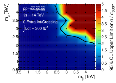
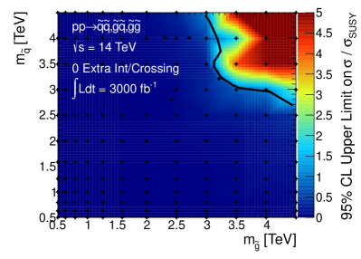
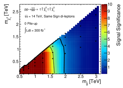
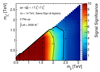
SUSY Simplified Models at
14, 33, and 100 TeV Proton Colliders

1 Introduction

The Large Hadron Collider (LHC) has completed its 888 TeV run. Searches for a wide variety of beyond the Standard Model (SM) states, both in the context of Supersymmetry (SUSY) and otherwise, have been (and are being) performed. The absence so far for any signatures of new particles lurking in the 8 TeV8 TeV8{\text{ TeV}} data does not deter the expectation that new physics will be accessible at colliders. The next stage of the energy frontier collider effort will begin once the LHC has completed its upgrade to a center-of-mass energy approaching 141414 TeV. In addition, discussions of collider physics beyond the LHC have begun; of particular relevance here are plans for a proton collider with s100 TeVsimilar-to𝑠100 TeV\sqrt{s}\sim 100{\text{ TeV}}. In light of all this activity, it is interesting to develop a quantitative picture for the physics potential of the next phase of the LHC and beyond.

This work provides a study of the reach of the LHC upgrade and future proton colliders in the context of SUSY Simplified Models [1, 2, 3]. Supersymmetry is one of the best-motivated possibilities for new physics within the reach of future machines. Supersymmetric models provide a framework for constructing collider searches that generically cover additional motivated extensions of the SM; most importantly signals that involve missing energy and/or heavy flavor production. Furthermore, there is a cornucopia of results on SUSY extensions to the SM using 8 TeV8 TeV8{\text{ TeV}} LHC data that provide a useful reference point for comparing the reach of future colliders. Clearly, assessing the ability to search for new physics in the context of SUSY is a convenient benchmark for understanding the general physics potential of future proton colliders.

Given the vast possibilities for signatures that can be realized within the SUSY framework, we choose to work with the signature driven approach of Simplified Models. The philosophy underlying Simplified Models is simple: isolate the minimal field content required to produce a specific SUSY signature — it then becomes tractable to optimize a search such that it provides the maximal reach in both mass and σ×BR𝜎BR\sigma\times\text{BR}. In practice, Simplified Models are IR-defined Lagrangian based theories that consist of a minimal number of particles and couplings; by keeping the number of free parameters to 𝒪(a few)𝒪a few\mathcal{O}(\text{a few}), it is possible to understand the consequences of a given experiment for the entire parameter space.

Note that Simplified Models do not capture certain features of “complete” SUSY models; this approach remains agnostic about complimentary phenomenology, e.g. dark matter. For contrast consider the UV-motivated simplified parameter space of the CMSSM; many of these models do contain multiple collider accessible particles, but it is only possible to explore the full parameter space with a non-trivial combination of experiments including proton colliders and dark matter detection [4]. Another fruitful approach for understanding complementarity between experiments is the reduced IR parameter space of the pMSSM [5]. However, it can be challenging to interpret and generalize the results of CMSSM or pMSSM specific collider searches to more generic settings.

The parameter space of SUSY Simplified Models has been explored in great detail at the 8 TeV LHC by both the ATLAS and CMS collaborations (for a recent overview of the experimental exclusions and the implications for SUSY models, see [6]). In this work we focus on minimal SUSY extensions of the SM with colored initial states. These models are expected to provide the greatest sparticle mass reach at hadron colliders.

In particular, motivated by expectations for the “first signatures” of SUSY, we study the following Simplified Models:

Section Simplified Model Decay Channel
3 and 4 Gluino-neutralino with light flavor decays g~qq¯χ~10~𝑔𝑞¯𝑞superscriptsubscript~𝜒10\widetilde{g}\rightarrow q\,\overline{q}\,\widetilde{\chi}_{1}^{0}
5 and 6 Squark-neutralino q~qχ~10~𝑞𝑞superscriptsubscript~𝜒10\widetilde{q}\rightarrow q\,\widetilde{\chi}_{1}^{0}
7 Gluino-squark with a massless neutralino g~(qq¯χ~10/qq~)~𝑔𝑞¯𝑞superscriptsubscript~𝜒10𝑞superscript~𝑞\widetilde{g}\rightarrow\big{(}q\,\overline{q}\,\widetilde{\chi}_{1}^{0}/q\,\widetilde{q}^{*}\big{)}; q~(qχ~10/qg~)~𝑞𝑞superscriptsubscript~𝜒10𝑞~𝑔\widetilde{q}\rightarrow\big{(}q\,\widetilde{\chi}_{1}^{0}/q\,\widetilde{g}\big{)}
8 Gluino-neutralino with heavy flavor decays g~tt¯χ~10~𝑔𝑡¯𝑡superscriptsubscript~𝜒10\widetilde{g}\rightarrow t\,\overline{t}\,\widetilde{\chi}_{1}^{0}

Our analyses loosely follow existing public 8 TeV search strategies from the ATLAS and CMS collaborations with optimizations performed to account for the higher luminosity and energy. We study the impact of pileup conditions to estimate how our conclusions could be altered by the harsh environments of running proton colliders at high instantaneous luminosity. Additional studies on the impact of systematic uncertainties are provided for a few models.

Discovery reach and exclusions limits are given for the following collider scenarios:

Machine s𝑠\sqrt{s} Final Integrated Luminosity
LHC Phase I 14 TeV14 TeV14\,{\text{ TeV}} 300300300 fb-1
HL-LHC or LHC Phase II 14 TeV14 TeV14\,{\text{ TeV}} 300030003000 fb-1
HE-LHC 33 TeV33 TeV33\,{\text{ TeV}} 300030003000 fb-1
VLHC 100 TeV100 TeV100\,{\text{ TeV}} 300030003000 fb-1

The results presented in this work use the common Snowmass backgrounds [7], which were generated using the Open Science Grid [8]. The Snowmass detector framework [9] was used for signal and background event reconstruction. QCD backgrounds were not simulated as the preselection cuts have been demonstrated to effectively eliminate any QCD contamination. Note that all results presented here are based on existing Monte Carlo and detector simulation tools extended to 33 TeV33 TeV33{\text{ TeV}} and 100 TeV100 TeV100{\text{ TeV}}. We do not investigate the uncertainties related to the extrapolation of parton distribution functions or the modeling of electroweak contributions to the parton shower at high collision energies (for some discussion of these issues, see the Snowmass report from the energy frontier QCD working group [10]).

While studies assuming center-of mass energies beyond 14 TeV14 TeV14{\text{ TeV}} do exist, for example the famous EHLQ paper on SSC collider physics [11], the results presented here represent some of the first computations that have been done using modern Monte Carlo and detector simulation tools. This work is a broad first step in the realistic assessment of the capabilities of future proton colliders for new particle searches, This work, along with other Snowmass 2013 studies of new physics searches at 33 TeV33 TeV33{\text{ TeV}} [12, 13, 14, 15] and 100 TeV100 TeV100{\text{ TeV}} [16, 17, 18, 19, 20, 21] colliders, provides a useful reference for evaluating future experimental options and a launching point for further detailed investigation.

The rest of the paper is organized as follows. Section 2 compares our results with an official 141414 TeV ATLAS study. The remaining sections are divided by the particular choice of Simplified Model, with separate sections for the searches targeted in the compressed regions of parameter space. Sections 3-7 describe the searches and results for Simplified Models with hadronic final states, with the details of the common analyses and the impact of pile-up and systematics discussed in the context of the gluino-neutralino model in Sec. 3 and for compressed spectra in Sec. 4. Section 8 presents the analysis and sensitivity of a leptonic search for the gluino-neutralino model with heavy flavor decays. An appendix provides the details of the Monte Carlo framework employed for this study.

A companion paper [22] provides a summary of the results and lessons learned. Its purpose is to emphasize the compelling case for future proton colliders.

2 Validation

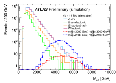
In order to validate our event generation and weighting procedures, we have made a comparison with an ATLAS study on the capabilities of the high luminosity 14 TeV LHC [23]. Specifically, ATLAS provides distributions for benchmark points in the gluino-squark plane with

  • mg~=3200 GeVsubscript𝑚~𝑔3200 GeVm_{\widetilde{g}}=3200{\text{ GeV}}; mq~=3200 GeVsubscript𝑚~𝑞3200 GeVm_{\widetilde{q}}=3200{\text{ GeV}}

  • mg~=2800 GeVsubscript𝑚~𝑔2800 GeVm_{\widetilde{g}}=2800{\text{ GeV}}; mq~=2400 GeVsubscript𝑚~𝑞2400 GeVm_{\widetilde{q}}=2400{\text{ GeV}}

where the following requirements are enforced: ETmiss/HT>15 GeV1/2superscriptsubscript𝐸𝑇misssubscript𝐻𝑇15superscript GeV12E_{T}^{\mathrm{miss}}/\sqrt{H_{T}}>15{\text{ GeV}}^{1/2}, no leptons, and four jets with pT>60 GeVsubscript𝑝𝑇60 GeVp_{T}>60{\text{ GeV}}.

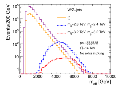
In the left panel of Fig. 1 we show the meffsubscript𝑚effm_{\text{eff}} distribution for signal and backgrounds from [23] and on the right we show our analogous distribution. The signal distributions are the same within the tolerance of the systematic uncertainty assumed below. We find that the parts of the distributions within the cut regions for our analyses appear to be consistent to within 10%. The ETmiss/HTsuperscriptsubscript𝐸𝑇misssubscript𝐻𝑇E_{T}^{\mathrm{miss}}/\sqrt{H_{T}} distribution, also provided in [23], is also consistent with our results. Finally, we note that while we use slightly different search strategies (and have used different detector simulations) we obtain similar results for the gluino-squark plane presented below in Sec. 7.
Refer to caption
Refer to caption
Figure 1: Plotted on the left [right] is the histogram of meffsubscript𝑚effm_{\text{eff}} for the validation model as determined by ATLAS [this study]. Note that an exact comparison between the background not possible since we use the Snowmass particle containers, i.e. W𝑊W + jets and Z𝑍Z + jets are plotted together. The background histograms are not stacked.

3 The Gluino-Neutralino Model with Light Flavor Decays

In the “gluino-neutralino model with light flavor decays”, the gluino g~~𝑔\widetilde{g} is the only kinematically accessible colored particle. The squarks are completely decoupled and do not contribute to gluino production diagrams. The gluino undergoes a prompt three-body decay through off-shell squarks, g~qq¯χ~10~𝑔𝑞¯𝑞subscriptsuperscript~𝜒01\widetilde{g}\rightarrow q\,\overline{q}\,\widetilde{\chi}^{0}_{1}, where q=u,d,c,s𝑞𝑢𝑑𝑐𝑠q=u,d,c,s are the first and second generation quarks and χ~10subscriptsuperscript~𝜒01\widetilde{\chi}^{0}_{1} is a neutralino LSP. The branching ratios to all four flavors of light quark are taken to be equal. The only two relevant parameters are the gluino mass mg~subscript𝑚~𝑔m_{\widetilde{g}} and the neutralino mass mχ~10subscript𝑚subscriptsuperscript~𝜒01m_{\widetilde{\chi}^{0}_{1}}. This model can be summarized by:

BSM particles production decays
g~,χ~10~𝑔subscriptsuperscript~𝜒01\widetilde{g},\,\widetilde{\chi}^{0}_{1} ppg~g~𝑝𝑝~𝑔~𝑔p\,p\rightarrow\widetilde{g}\,\widetilde{g} g~qq¯χ~10~𝑔𝑞¯𝑞subscriptsuperscript~𝜒01\widetilde{g}\rightarrow q\,\overline{q}\,\widetilde{\chi}^{0}_{1}

This model is motivated by (mini-)split supersymmetry scenarios, where the scalar superpartners are heavier than the gauginos [24, 25, 26, 27, 28]. The final state is four (or more) hard jets and missing energy. Therefore, this signature provides a good proxy with which to investigate the power of a traditional jets plus ETmisssuperscriptsubscript𝐸𝑇missE_{T}^{\mathrm{miss}} style hadron collider search strategy to discriminate against background. The current preliminary limits on this model using 202020 fb-1 of 888 TeV data are mg~=1350 GeVsubscript𝑚~𝑔1350 GeVm_{\widetilde{g}}=1350\text{ GeV} (ATLAS [29]) and mg~=1200 GeVsubscript𝑚~𝑔1200 GeVm_{\widetilde{g}}=1200\text{ GeV} (CMS [30]) assuming a massless neutralino.

We simulated matched MadGraph samples for g~g~~𝑔~𝑔\widetilde{g}\,\widetilde{g} with up to 2 additional generator level jets for the following points in parameter space:111We include 1 GeV1 GeV1{\text{ GeV}} for an example where the neutralino is effectively massless; the second line of neutralino masses is chosen to cover the bulk of the gluino-neutralino plane; the final line is chosen to ensure coverage in the “compressed” region.

BSM particles masses
mg~subscript𝑚~𝑔m_{\widetilde{g}} [14 TeV]delimited-[]14 TeV\big{[}14{\text{ TeV}}\big{]} (315,397,500,629,792,997,1255,1580,1989,2489,2989,3489) GeV315397500629792997125515801989248929893489 GeV(315,397,500,629,792,997,1255,1580,1989,2489,2989,3489){\text{ GeV}}
mg~subscript𝑚~𝑔m_{\widetilde{g}} [33 TeV]delimited-[]33 TeV\big{[}33{\text{ TeV}}\big{]} (500,629,792,997,1255,1580,1989,2504,3152,(500,629,792,997,1255,1580,1989,2504,3152,
3968,4968,5968,6968) GeV3968,4968,5968,6968){\text{ GeV}}
mg~subscript𝑚~𝑔m_{\widetilde{g}} [100 TeV]delimited-[]100 TeV\big{[}100{\text{ TeV}}\big{]} (1000,1259,1585,1995,2512,3162,3981,5012,6310,(1000,1259,1585,1995,2512,3162,3981,5012,6310,
7944,9944,11944,13944,15944) GeV7944,9944,11944,13944,15944){\text{ GeV}}
1 GeV1 GeV1{\text{ GeV}}
mχ~10subscript𝑚subscriptsuperscript~𝜒01m_{\widetilde{\chi}^{0}_{1}} (0.2,0.4,0.6,0.7,0.8,0.9)×mg~0.20.40.60.70.80.9subscript𝑚~𝑔(0.2,0.4,0.6,0.7,0.8,0.9)\times m_{\widetilde{g}}
mg~(100 GeV,50 GeV,15 GeV,5 GeV)subscript𝑚~𝑔100 GeV50 GeV15 GeV5 GeVm_{\widetilde{g}}-(100{\text{ GeV}},50{\text{ GeV}},15{\text{ GeV}},5{\text{ GeV}})

We find that including pileup does not significantly change the results of this study and present results below for only the no-pileup case. We discuss the effect of pile-up in more detail in Sec. 3.12.

3.1 Dominant Backgrounds

The background is dominated by W/Z+jets𝑊𝑍jetsW/Z+\text{jets}, with subdominant contributions from tt¯𝑡¯𝑡t\,\overline{t} production. Single top events and W/Z𝑊𝑍W/Z events from vector boson fusion processes are also illustrated in several figures, and are negligible. In all cases, there are decay modes which lead to multi-jet signatures. The ETmisssuperscriptsubscript𝐸𝑇missE_{T}^{\mathrm{miss}} can come from a variety of sources, such as neutrinos, jets/leptons which are lost down the beam pipe, and energy smearing effects.

3.2 Analysis Strategy

The gluino-neutralino model with light flavor decays can be probed with an analysis inspired by the ATLAS analysis in [23]. After an event preselection, rectangular cuts on one or more variables are optimized at each point in parameter space to yield maximum signal significance. Specifically, we simultaneously scan a two-dimensional set of cuts on ETmisssuperscriptsubscript𝐸𝑇missE_{T}^{\mathrm{miss}} and HTsubscript𝐻𝑇H_{T}, where ETmisssuperscriptsubscript𝐸𝑇missE_{T}^{\mathrm{miss}} is the magnitude of the missing transverse momentum and HTsubscript𝐻𝑇H_{T} is defined as the scalar sum of jet pTsubscript𝑝𝑇p_{T} . In contrast, the discriminating variable used by ATLAS is meffsubscript𝑚effm_{\text{eff}}, the scalar sum of HTsubscript𝐻𝑇H_{T} and ETmisssuperscriptsubscript𝐸𝑇missE_{T}^{\mathrm{miss}}. We require jets to have pT>30subscript𝑝𝑇30p_{T}>30 GeV and |η|<3.5𝜂3.5|\eta|<3.5. Electrons and muons are selected by requiring pT>10subscript𝑝𝑇10p_{T}>10 GeV and |η|<2.6𝜂2.6|\eta|<2.6.

In detail, our analysis strategy proceeds as follows:

Preselection

  • zero selected electrons or muons

  • ETmiss>100superscriptsubscript𝐸𝑇miss100E_{T}^{\mathrm{miss}}>100 GeV

  • at least 4 jets with pT>60subscript𝑝𝑇60p_{T}>60 GeV

After preselection, a requirement is placed on ETmiss/HTsuperscriptsubscript𝐸𝑇misssubscript𝐻𝑇E_{T}^{\mathrm{miss}}/\sqrt{H_{T}} to further reduce the QCD background, where the dominant source of ETmisssuperscriptsubscript𝐸𝑇missE_{T}^{\mathrm{miss}} is from jet mismeasurement. A cut on the leading jet pTsubscript𝑝𝑇p_{T} is applied to reduce backgrounds from hard ISR jets. Finally, a two dimensional scan over cuts on HTsubscript𝐻𝑇H_{T} and ETmisssuperscriptsubscript𝐸𝑇missE_{T}^{\mathrm{miss}}is performed to determine the maximum significance.

Search Strategy: Simultaneous optimization over HTsubscript𝐻𝑇H_{T} and ETmisssuperscriptsubscript𝐸𝑇missE_{T}^{\mathrm{miss}}

  • ETmiss/HT>15superscriptsubscript𝐸𝑇misssubscript𝐻𝑇15E_{T}^{\mathrm{miss}}/\sqrt{H_{T}}>15 GeV1/2

  • The leading jet pTsubscript𝑝𝑇p_{T} must satisfy pTleading<0.4HTsuperscriptsubscript𝑝𝑇leading0.4subscript𝐻𝑇p_{T}^{\text{leading}}<0.4\,H_{T}

  • ETmiss>(ETmiss)optimalsuperscriptsubscript𝐸𝑇misssubscriptsuperscriptsubscript𝐸𝑇missoptimalE_{T}^{\mathrm{miss}}>(E_{T}^{\mathrm{miss}})_{\text{optimal}}

  • HT>(HT)optimalsubscript𝐻𝑇subscriptsubscript𝐻𝑇optimalH_{T}>(H_{T})_{\text{optimal}}

The 141414, 333333, and 100100100 TeV analyses all use the same set of fixed cuts, differing only in the optimization over (ETmiss)optimalsubscriptsuperscriptsubscript𝐸𝑇missoptimal(E_{T}^{\mathrm{miss}})_{\text{optimal}} and (HT)optimalsubscriptsubscript𝐻𝑇optimal(H_{T})_{\text{optimal}}. In practice, scaling the ETmiss/HTsuperscriptsubscript𝐸𝑇misssubscript𝐻𝑇E_{T}^{\mathrm{miss}}/\sqrt{H_{T}} cut with CM energy may be desirable to reduce QCD background, and we have verified that this has no effect on the efficiencies for the signal and dominant backgrounds for the models under study.

Note that this search yields some power to discover these models in the difficult region of parameter space where the neutralino is degenerate with the gluino. Section 4 will provide the results of a search that is specifically targeted for this region of parameter space.

3.3   Analysis: 14 TeV

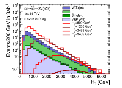
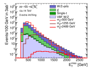
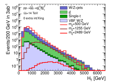
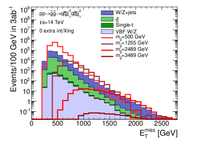
In Fig. 2 we show histograms of ETmisssuperscriptsubscript𝐸𝑇missE_{T}^{\mathrm{miss}} [left] and HTsubscript𝐻𝑇H_{T} [right] for signal and background at s=14 TeV𝑠14 TeV\sqrt{s}=14{\text{ TeV}} after applying the preselection cuts listed in Sec. 3.2. Because the tails of the signal and background distributions have a similar slope, the optimization procedure generally leads to cuts near the bulk of the signal distribution. We find that the searches are systematics limited when the optimal cuts are applied (see Sec. 3.11 below for a detailed discussion).

Using the search strategy discussed above in Sec. 3.2, it is possible to explore the potential reach for the gluino-neutralino model at the 14 TeV LHC. Table 1 gives a few example of the number of events that result from this cut flow for background and three example signal points: mg~=500, 1255, and 2489 GeVsubscript𝑚~𝑔5001255 and 2489 GeVm_{\widetilde{g}}=500,\,1255,\text{ and }2489{\text{ GeV}} with mχ~10=1 GeVsubscript𝑚subscriptsuperscript~𝜒011 GeVm_{\widetilde{\chi}^{0}_{1}}=1{\text{ GeV}}. Each choice of the ETmisssuperscriptsubscript𝐸𝑇missE_{T}^{\mathrm{miss}} and HTsubscript𝐻𝑇H_{T} cuts given in Table 1 corresponds to the optimal cut for one of the given signal points. The hardness of the cut increases with the mass of the gluino. Note that for 141414 TeV proton collisions, the V𝑉V+jets background dominates over the events from tt¯𝑡¯𝑡t\,\overline{t}. From this table, it is possible to infer that 500 GeV500 GeV500{\text{ GeV}} and 1255 GeV1255 GeV1255{\text{ GeV}} gluinos could be easily discovered while the 2489 GeV2489 GeV2489{\text{ GeV}} would only yield a few σ𝜎\sigma hint using the full power of the high luminosity LHC.
Refer to caption
Refer to caption
Figure 2: Histogram of ETmisssuperscriptsubscript𝐸𝑇missE_{T}^{\mathrm{miss}} [left] and HTsubscript𝐻𝑇H_{T} [right] after preselection cuts for background and a range of gluino-neutralino models with light flavor decays at the 141414 TeV LHC. The neutralino mass is 1 GeV1 GeV1{\text{ GeV}} for all signal models.
mg~subscript𝑚~𝑔m_{\widetilde{g}} [GeV]
Cut V𝑉V+jets tt¯𝑡¯𝑡t\bar{t} Total BG 500 1255 2489
PreselectionPreselection\mathrm{Preselection} 2.07×1072.07superscript1072.07\times 10^{7} 2.47×1072.47superscript1072.47\times 10^{7} 4.54×1074.54superscript1074.54\times 10^{7} 3.08×1073.08superscript1073.08\times 10^{7} 1.03×1051.03superscript1051.03\times 10^{5} 173
ETmiss/HT>15 GeV1/2superscriptsubscript𝐸𝑇misssubscript𝐻𝑇15superscript GeV12E_{T}^{\mathrm{miss}}/\sqrt{H_{T}}>15\text{ GeV}^{1/2} 4.45×1054.45superscript1054.45\times 10^{5} 1.20×1051.20superscript1051.20\times 10^{5} 5.65×1055.65superscript1055.65\times 10^{5} 1.34×1061.34superscript1061.34\times 10^{6} 3.14×1043.14superscript1043.14\times 10^{4} 95
pTleading<0.4×HTsuperscriptsubscript𝑝Tleading0.4subscript𝐻𝑇p_{\mathrm{T}}^{\mathrm{leading}}<0.4\times H_{T} 1.69×1051.69superscript1051.69\times 10^{5} 5.16×1045.16superscript1045.16\times 10^{4} 2.21×1052.21superscript1052.21\times 10^{5} 7.62×1057.62superscript1057.62\times 10^{5} 1.68×1041.68superscript1041.68\times 10^{4} 52.9
ETmiss>450superscriptsubscript𝐸𝑇miss450E_{T}^{\mathrm{miss}}>450 GeV 4.73×1044.73superscript1044.73\times 10^{4} 1.84×1041.84superscript1041.84\times 10^{4} 6.57×1046.57superscript1046.57\times 10^{4} 5.57×1055.57superscript1055.57\times 10^{5} 2.98×1042.98superscript1042.98\times 10^{4} 115
HT>800subscript𝐻𝑇800H_{T}>800 GeV
ETmiss>800superscriptsubscript𝐸𝑇miss800E_{T}^{\mathrm{miss}}>800 GeV 1.22×1031.22superscript1031.22\times 10^{3} 554 1.78×1031.78superscript1031.78\times 10^{3} 1.14×1041.14superscript1041.14\times 10^{4} 9.36×1039.36superscript1039.36\times 10^{3} 110
HT>1650subscript𝐻𝑇1650H_{T}>1650 GeV
ETmiss>1050superscriptsubscript𝐸𝑇miss1050E_{T}^{\mathrm{miss}}>1050 GeV 55.5 30.1 85.6 297 288 57.2
HT>2600subscript𝐻𝑇2600H_{T}>2600 GeV
Table 1: Number of expected events for s=14𝑠14\sqrt{s}=14 TeV with 3000 fb-1 integrated luminosity for the background processes and selected gluino masses for the gluino-neutralino model with light flavor decays. The neutralino mass is 1 GeV1 GeV1{\text{ GeV}}. Three choices of cuts on ETmisssuperscriptsubscript𝐸𝑇missE_{T}^{\mathrm{miss}} and HTsubscript𝐻𝑇H_{T} are provided, and for each gluino mass column the entry in the row corresponding to the “optimal” cuts is marked in red.

3.4   Results: 14 TeV

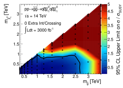
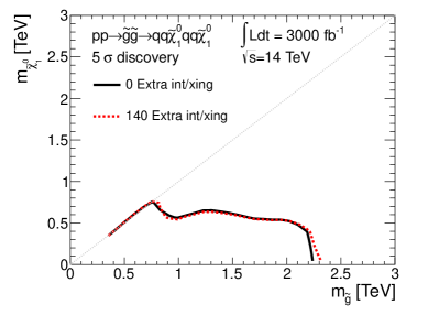
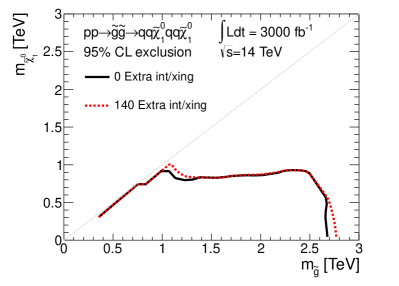
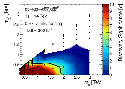
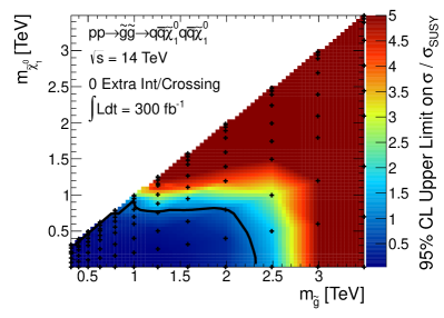
The 5σ5𝜎5\sigma discovery [top] and 95%percent9595\% CL limits [bottom] for the gluino-neutralino model are shown in Fig. 3. The left [right] panel assumes 300 fb1300superscript fb1300\text{ fb}^{-1} [3000 fb1]delimited-[]3000superscript fb1\left[3000\text{ fb}^{-1}\right] of integrated luminosity. The signal and background yields after optimized cuts are provided as inputs to a RooStats routine to calculate 95% CL exclusion intervals using the CLs method along with the expected signal p0subscript𝑝0p_{0} values. A 20%percent2020\% systematic uncertainty is applied to the backgrounds. The assumed signal systematics are outlined in the appendix.

Using the NLO gluino pair production cross section one can make a very naive estimate for the reach of a given collider. For example, we find that the choice of gluino mass which would yield 101010 events at 300 fb1300superscript fb1300\text{ fb}^{-1} (3000 fb1)3000superscript fb1\big{(}3000\text{ fb}^{-1}\big{)} is 2.8(3.3) TeV2.83.3 TeV2.8\,(3.3){\text{ TeV}}. This roughly corresponds to the maximal possible reach one could expect for a given luminosity using 14 TeV14 TeV14{\text{ TeV}} proton collisions.

Using a realistic simulation framework along with the search strategy employed here, the 14 TeV14 TeV14{\text{ TeV}} 300 fb1300superscript fb1300\text{ fb}^{-1} limit with massless neutralinos is projected to be at a gluino mass of 2.3 TeV2.3 TeV2.3{\text{ TeV}} (corresponding to 110 events), while the 14 TeV14 TeV14{\text{ TeV}} 3000 fb13000superscript fb13000\text{ fb}^{-1} limit is projected to be at 2.7 TeV2.7 TeV2.7{\text{ TeV}} (corresponding to 175 events). Furthermore, the 14 TeV14 TeV14{\text{ TeV}} LHC with 3000 fb13000superscript fb13000\text{ fb}^{-1} could discover a gluino as heavy as 2.3 TeV2.3 TeV2.3{\text{ TeV}} if the neutralino is massless, while for mχ~10500 GeVgreater-than-or-equivalent-tosubscript𝑚subscriptsuperscript~𝜒01500 GeVm_{\widetilde{\chi}^{0}_{1}}\gtrsim 500{\text{ GeV}} the gluino mass reach rapidly diminishes.
Refer to caption
Refer to caption
Refer to caption
Refer to caption
Figure 3: Results at 14 TeV14 TeV14{\text{ TeV}} for the gluino-neutralino model with light flavor decays are given in the mχ~10subscript𝑚subscriptsuperscript~𝜒01m_{\widetilde{\chi}^{0}_{1}} versus mg~subscript𝑚~𝑔m_{\widetilde{g}} plane. The top [bottom] row shows the expected 5σ5𝜎5\sigma discovery reach [95% confidence level upper limits] for gluino pair production. Mass points to the left/below the contours are expected to be probed at 300 fb1300superscript fb1300\text{ fb}^{-1} [left] and 3000 fb13000superscript fb13000\text{ fb}^{-1} [right]. A 20% systematic uncertainty is assumed and pileup is not included. The black crosses mark the simulated models.

3.5   Analysis: 33 TeV

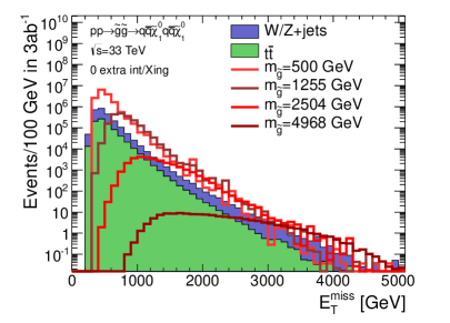
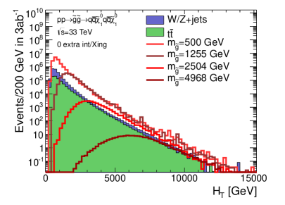
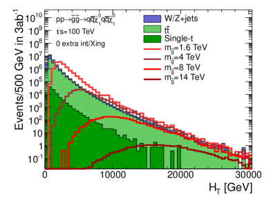
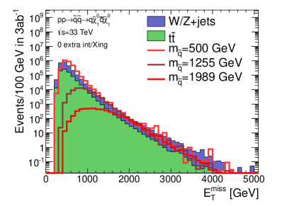
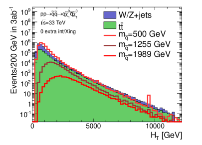
In Fig. 4 we show histograms of ETmisssuperscriptsubscript𝐸𝑇missE_{T}^{\mathrm{miss}} [left] and HTsubscript𝐻𝑇H_{T} [right] for signal and background at s=33 TeV𝑠33 TeV\sqrt{s}=33{\text{ TeV}} after applying the preselection cuts listed in Sec. 3.2. Because the tails of the signal and background distributions have a similar slope, the optimization procedure generally leads to cuts near the bulk of the signal distribution. Moving to a higher center-of-mass energy allows for harder cuts to be placed, which in turn implies fewer background events survive the requirements. At 333333 TeV, we find that the searches are systematics limited when the optimal cuts are applied (see Sec. 3.11 below for a detailed discussion).

Refer to caption
Refer to caption
Figure 4: Histogram of ETmisssuperscriptsubscript𝐸𝑇missE_{T}^{\mathrm{miss}} [left] and HTsubscript𝐻𝑇H_{T} [right] after preselection cuts for background and a range of gluino-neutralino models with light flavor decays at a 333333 TeV proton collider. The neutralino mass is 1 GeV1 GeV1{\text{ GeV}} for all signal models.

Using the search strategy discussed above in Sec. 3.2, it is possible to explore the potential reach for the gluino-neutralino model at a 333333 TeV proton collider. Table 2 gives a few example of the number of events that result from this cut flow for background and three example signal points: mg~=1255, 3152, and 4968 GeVsubscript𝑚~𝑔12553152 and 4968 GeVm_{\widetilde{g}}=1255,\,3152,\text{ and }4968{\text{ GeV}} with mχ~10=1 GeVsubscript𝑚subscriptsuperscript~𝜒011 GeVm_{\widetilde{\chi}^{0}_{1}}=1{\text{ GeV}}. Each choice of the ETmisssuperscriptsubscript𝐸𝑇missE_{T}^{\mathrm{miss}} and HTsubscript𝐻𝑇H_{T} cuts given in Table 2 corresponds to the optimal cuts for one of the given signal points. The hardness of the cut increases with the mass of the gluino. It is clear that the ratio of tt¯𝑡¯𝑡t\,\overline{t} to V+limit-from𝑉V+jets background is growing with regards to the 141414 TeV search; this is due to the higher probability for gluon scattering as s𝑠\sqrt{s} increases. It would likely be advantageous to veto b𝑏b-tagged jets to further reduce the background from top quarks, and similarly to veto τ𝜏\tau-tagged jets to further reduce W/Z𝑊𝑍W/Z+jets. From this table, it is possible to infer that gluinos as heavy as 5similar-toabsent5\sim 5 TeV could be discovered at a 333333 TeV collider. HTsubscript𝐻𝑇H_{T} cuts as hard as 555 TeV are required to extract the most information from this data set.

mg~subscript𝑚~𝑔m_{\widetilde{g}} [GeV]
Cut V𝑉V+jets tt¯𝑡¯𝑡t\overline{t} Total BG 125512551255 315231523152 496849684968
PreselectionPreselection\mathrm{Preselection} 1.55×1081.55superscript1081.55\times 10^{8} 2.86×1082.86superscript1082.86\times 10^{8} 4.42×1084.42superscript1084.42\times 10^{8} 1.22×1071.22superscript1071.22\times 10^{7} 1.89×1041.89superscript1041.89\times 10^{4} 316316316
ETmiss/HT>15 GeV1/2superscriptsubscript𝐸𝑇misssubscript𝐻𝑇15superscript GeV12E_{T}^{\mathrm{miss}}/\sqrt{H_{T}}>15{\text{ GeV}}^{1/2} 4.50×1064.50superscript1064.50\times 10^{6} 1.93×1061.93superscript1061.93\times 10^{6} 6.44×1066.44superscript1066.44\times 10^{6} 3.50×1063.50superscript1063.50\times 10^{6} 1.13×1041.13superscript1041.13\times 10^{4} 229
pTleading<0.4×HTsuperscriptsubscript𝑝𝑇leading0.4subscript𝐻𝑇p_{T}^{\mathrm{leading}}<0.4\times H_{T} 1.70×1061.70superscript1061.70\times 10^{6} 8.02×1058.02superscript1058.02\times 10^{5} 2.50×1062.50superscript1062.50\times 10^{6} 1.94×1061.94superscript1061.94\times 10^{6} 6.94×1036.94superscript1036.94\times 10^{3} 139
ETmiss>900 GeVsuperscriptsubscript𝐸𝑇miss900 GeVE_{T}^{\mathrm{miss}}>900{\text{ GeV}} 4.06×1044.06superscript1044.06\times 10^{4} 5.65×1045.65superscript1045.65\times 10^{4} 9.71×1049.71superscript1049.71\times 10^{4} 8.36×1058.36superscript1058.36\times 10^{5} 6.93×1036.93superscript1036.93\times 10^{3} 139139139
HT>1900 GeVsubscript𝐻𝑇1900 GeVH_{T}>1900{\text{ GeV}}
ETmiss>2100 GeVsuperscriptsubscript𝐸𝑇miss2100 GeVE_{T}^{\mathrm{miss}}>2100{\text{ GeV}} 127127127 103103103 230230230 1.44×1031.44superscript1031.44\times 10^{3} 1.10×1031.10superscript1031.10\times 10^{3} 78.578.578.5
HT>3800 GeVsubscript𝐻𝑇3800 GeVH_{T}>3800{\text{ GeV}}
ETmiss>2750 GeVsuperscriptsubscript𝐸𝑇miss2750 GeVE_{T}^{\mathrm{miss}}>2750{\text{ GeV}} 101010 7.87.87.8 17.817.817.8 53.153.153.1 91.291.291.2 33.633.633.6
HT>5150 GeVsubscript𝐻𝑇5150 GeVH_{T}>5150{\text{ GeV}}
Table 2: Number of expected events for s=33𝑠33\sqrt{s}=33 TeV with 3000 fb-1 integrated luminosity for the background processes and selected gluino masses for the gluino-neutralino model with light flavor decays. The neutralino mass is 1 GeV1 GeV1{\text{ GeV}}. Three choices of cuts on ETmisssuperscriptsubscript𝐸𝑇missE_{T}^{\mathrm{miss}} and HTsubscript𝐻𝑇H_{T} are provided, and for each gluino mass column the entry in the row corresponding to the “optimal” cuts is marked in red.

3.6   Results: 33 TeV

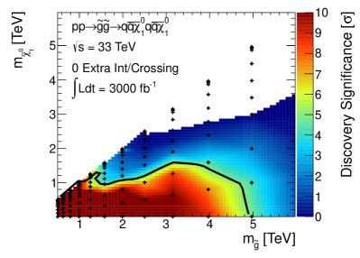
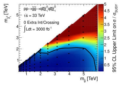
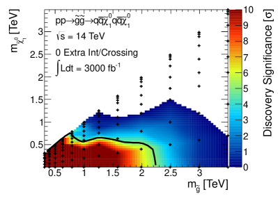
The 5σ5𝜎5\sigma discovery [left] and 95%percent9595\% C.L. limits [right] for the gluino-neutralino model are shown in Fig. 5, assuming 3000 fb13000superscript fb13000\text{ fb}^{-1} of integrated luminosity. 20%percent2020\% systematic uncertainty is applied to the backgrounds. The assumed signal systematic are outlined in the appendix. Pileup is not included; a demonstration that pileup will not significantly change these results is given in Sec. 3.12 below.

Using the NLO gluino pair production cross section one can make a very naive estimate for the reach of a given collider. For example, we find that the choice of gluino mass which would yield 101010 events at 3000 fb13000superscript fb13000\text{ fb}^{-1} is 6.7 TeV6.7 TeV6.7{\text{ TeV}}. This roughly corresponds to the maximal possible reach one could expect for a given luminosity using 33 TeV33 TeV33{\text{ TeV}} proton collisions.

Using a realistic simulation framework along with the search strategy employed here the 33 TeV33 TeV33{\text{ TeV}} 3000 fb13000superscript fb13000\text{ fb}^{-1} limit with massless neutralinos is projected to be 5.8 TeV5.8 TeV5.8{\text{ TeV}} (corresponding to 61 events). Furthermore, the 33 TeV33 TeV33{\text{ TeV}} proton collider with 3000 fb13000superscript fb13000\text{ fb}^{-1} could discover a gluino as heavy as 4.8 TeV4.8 TeV4.8{\text{ TeV}} if the neutralino is massless, while for mχ~101 TeVgreater-than-or-equivalent-tosubscript𝑚subscriptsuperscript~𝜒011 TeVm_{\widetilde{\chi}^{0}_{1}}\gtrsim 1{\text{ TeV}} the gluino mass reach rapidly diminishes.
Refer to caption
Refer to caption
Figure 5: Results at 33 TeV33 TeV33{\text{ TeV}} for the gluino-neutralino model with light flavor decays are given in the mχ~10subscript𝑚subscriptsuperscript~𝜒01m_{\widetilde{\chi}^{0}_{1}} versus mg~subscript𝑚~𝑔m_{\widetilde{g}} plane. The left [right] plot shows the expected 5σ5𝜎5\sigma discovery reach [95% confidence level upper limits] for gluino pair production. Mass points to the left/below the contours are expected to be probed at 3000 fb13000superscript fb13000\text{ fb}^{-1}. A 20% systematic uncertainty is assumed and pileup is not included. The black crosses mark the simulated models.

3.7   Analysis: 100 TeV

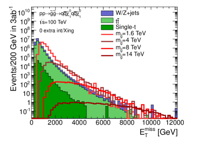
In Fig. 6 we show histograms of ETmisssuperscriptsubscript𝐸𝑇missE_{T}^{\mathrm{miss}} [left] and HTsubscript𝐻𝑇H_{T} [right] for signal and background at s=100 TeV𝑠100 TeV\sqrt{s}=100{\text{ TeV}} after applying the preselection cuts listed in Sec. 3.2. Because the tails of the signal and background distributions have a similar slope, the optimization procedure generally leads to cuts near the bulk of the signal distribution. Moving to a higher center-of-mass energy allows for harder cuts to be placed, which in turn implies fewer background events survive the requirements. For example, we find that the signal efficiencies at the high gluino mass edge of our limits are several times larger at 100 TeV100 TeV100{\text{ TeV}} than at 14 TeV14 TeV14{\text{ TeV}}. We find that the searches are only barely systematics limited when the optimal cuts are applied (see Sec. 3.11 below for a detailed discussion).

Refer to caption
Refer to caption
Figure 6: Histogram of ETmisssuperscriptsubscript𝐸𝑇missE_{T}^{\mathrm{miss}} [left] and HTsubscript𝐻𝑇H_{T} [right] after preselection cuts for background and a range of gluino-neutralino models with light flavor decays at a 100100100 TeV proton collider. The neutralino mass is 1 GeV1 GeV1{\text{ GeV}} for all signal models.

Using the search strategy discussed above in Sec. 3.2, it is possible to explore the potential reach for the gluino-neutralino model at a 100100100 TeV proton collider. Table 3 gives a few example of the number of events that result from this cut flow for background and three example signal points: mg~=5012, 9944, and 13944 GeVsubscript𝑚~𝑔50129944 and 13944 GeVm_{\widetilde{g}}=5012,\,9944,\text{ and }13944{\text{ GeV}} with mχ~10=1 GeVsubscript𝑚subscriptsuperscript~𝜒011 GeVm_{\widetilde{\chi}^{0}_{1}}=1{\text{ GeV}}. Each choice of the ETmisssuperscriptsubscript𝐸𝑇missE_{T}^{\mathrm{miss}} and HTsubscript𝐻𝑇H_{T} cuts given in Table 3 corresponds to the optimal cuts for one of the given signal points. The hardness of the cut increases with the mass of the gluino. It is clear that the ratio of tt¯𝑡¯𝑡t\,\overline{t} to V+limit-from𝑉V+jets background is growing with regards to the 141414 and 333333 TeV searches; this is due to the higher probability for gluon scattering as s𝑠\sqrt{s} increases. In this analysis it would certainly be advantageous to veto b𝑏b-tagged jets to further reduce the background from top quarks. From this table, it is possible to infer that gluinos as heavy as 10similar-toabsent10\sim 10 TeV could be discovered at a 100100100 TeV collider. HTsubscript𝐻𝑇H_{T} cuts as hard as 121212 TeV are required to extract the most information from this data set.

mg~subscript𝑚~𝑔m_{\widetilde{g}} [GeV]
Cut V𝑉V+jets tt¯𝑡¯𝑡t\overline{t} Total BG 501250125012 994499449944 139441394413944
PreselectionPreselection\mathrm{Preselection} 1.64×1091.64superscript1091.64\times 10^{9} 3.33×1093.33superscript1093.33\times 10^{9} 4.97×1094.97superscript1094.97\times 10^{9} 1.12×1051.12superscript1051.12\times 10^{5} 876876876 43.443.443.4
ETmiss/HT>15 GeV1/2superscriptsubscript𝐸𝑇misssubscript𝐻𝑇15superscript GeV12E_{T}^{\mathrm{miss}}/\sqrt{H_{T}}>15{\text{ GeV}}^{1/2} 3.59×1073.59superscript1073.59\times 10^{7} 3.31×1073.31superscript1073.31\times 10^{7} 6.90×1076.90superscript1076.90\times 10^{7} 7.99×1047.99superscript1047.99\times 10^{4} 740740740 38.838.838.8
pTleading<0.4×HTsuperscriptsubscript𝑝𝑇leading0.4subscript𝐻𝑇p_{T}^{\mathrm{leading}}<0.4\times H_{T} 1.19×1071.19superscript1071.19\times 10^{7} 1.25×1071.25superscript1071.25\times 10^{7} 2.44×1072.44superscript1072.44\times 10^{7} 4.87×1044.87superscript1044.87\times 10^{4} 443443443 22.722.722.7
ETmiss>5150 GeVsuperscriptsubscript𝐸𝑇miss5150 GeVE_{T}^{\mathrm{miss}}>5150{\text{ GeV}} 21.621.621.6 33.133.133.1 54.854.854.8 216216216 91.691.691.6 10.710.710.7
HT>9550 GeVsubscript𝐻𝑇9550 GeVH_{T}>9550{\text{ GeV}}
ETmiss>5530 GeVsuperscriptsubscript𝐸𝑇miss5530 GeVE_{T}^{\mathrm{miss}}>5530{\text{ GeV}} 121212 18.918.918.9 30.930.930.9 136136136 67.467.467.4 9.29.29.2
HT>9750 GeVsubscript𝐻𝑇9750 GeVH_{T}>9750{\text{ GeV}}
ETmiss>6150 GeVsuperscriptsubscript𝐸𝑇miss6150 GeVE_{T}^{\mathrm{miss}}>6150{\text{ GeV}} 4.14.14.1 6.36.36.3 10.410.410.4 33.633.633.6 29.629.629.6 6.86.86.8
HT>11700 GeVsubscript𝐻𝑇11700 GeVH_{T}>11700{\text{ GeV}}
Table 3: Number of expected events for s=100𝑠100\sqrt{s}=100 TeV with 3000 fb-1 integrated luminosity for the background processes and selected gluino masses for the gluino-neutralino model with light flavor decays. The neutralino mass is 1 GeV1 GeV1{\text{ GeV}}. Three choices of cuts on ETmisssuperscriptsubscript𝐸𝑇missE_{T}^{\mathrm{miss}} and HTsubscript𝐻𝑇H_{T} are provided, and for each gluino mass column the entry in the row corresponding to the “optimal” cuts is marked in red.

3.8   Results: 100 TeV

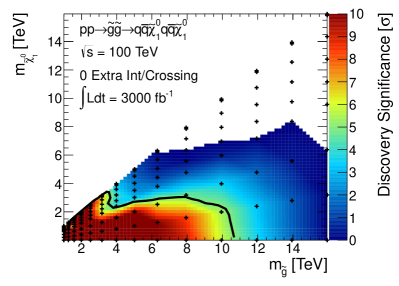
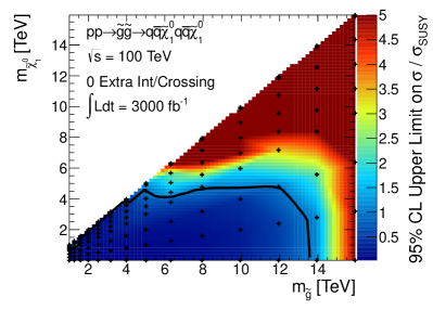
The 5σ5𝜎5\sigma discovery [left] and 95%percent9595\% CL limits [right] for the gluino-neutralino model are shown in Fig. 7, assuming 3000 fb13000superscript fb13000\text{ fb}^{-1} of integrated luminosity. 20%percent2020\% systematic uncertainty is applied to the backgrounds. The assumed signal systematic are outlined in the appendix. Pileup is not included; a demonstration that pileup will not significantly change these results is given in Sec. 3.12 below.

Using the NLO gluino pair production cross section one can make a very naive estimate for the reach of a given collider. For example, we find that the choice of gluino mass which would yield 101010 events at 3000 fb13000superscript fb13000\text{ fb}^{-1} is 16.1 TeV16.1 TeV16.1{\text{ TeV}}. This roughly corresponds to the maximal possible reach one could expect for a given luminosity using 100 TeV100 TeV100{\text{ TeV}} proton collisions.

Using a realistic simulation framework along with the search strategy employed here the 100 TeV100 TeV100{\text{ TeV}} 3000 fb13000superscript fb13000\text{ fb}^{-1} limit with massless neutralinos is projected to be 13.5 TeV13.5 TeV13.5{\text{ TeV}} (corresponding to 60 events). Furthermore, the 100 TeV100 TeV100{\text{ TeV}} proton collider with 3000 fb13000superscript fb13000\text{ fb}^{-1} could discover a gluino as heavy as 11 TeV11 TeV11{\text{ TeV}} if the neutralino is massless, while for mχ~101 TeVgreater-than-or-equivalent-tosubscript𝑚subscriptsuperscript~𝜒011 TeVm_{\widetilde{\chi}^{0}_{1}}\gtrsim 1{\text{ TeV}} the gluino mass reach rapidly diminishes.
The next section provides a comparison of the impact that the four Snowmass collider scenarios can have on the parameter space of this model.
Refer to caption
Refer to caption
Figure 7: Results at 100 TeV100 TeV100{\text{ TeV}} for the gluino-neutralino model with light flavor decays are given in the mχ~10subscript𝑚subscriptsuperscript~𝜒01m_{\widetilde{\chi}^{0}_{1}} versus mg~subscript𝑚~𝑔m_{\widetilde{g}} plane. The left [right] plot shows the expected 5σ5𝜎5\sigma discovery reach [95% confidence level upper limits] for gluino pair production. Mass points to the left/below the contours are expected to be probed at 3000 fb13000superscript fb13000\text{ fb}^{-1}. A 20% systematic uncertainty is assumed and pileup is not included. The black crosses mark the simulated models.

3.9   Comparing Colliders

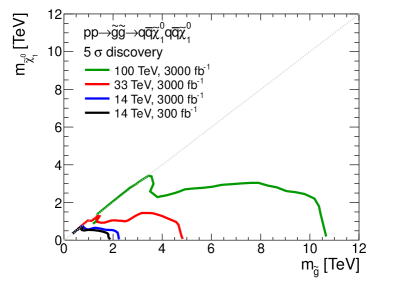
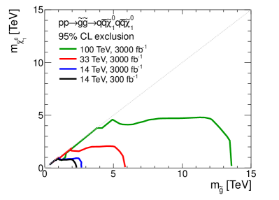
The multi-jet plus ETmisssuperscriptsubscript𝐸𝑇missE_{T}^{\mathrm{miss}} signature of the gluino-neutralino model with light flavor decays provides a useful study with which to compare the potential impact of different proton colliders. Figure 8 shows the 5σ5𝜎5\sigma discovery reach [95%percent9595\% CL exclusion] for two choices of integrated luminosity at 141414 TeV, along with the full data set assumed for 333333 and 100100100 TeV. At 141414 TeV, the factor of 101010 increase in luminosity leads to a modest increase by 350 GeV350 GeV350{\text{ GeV}} in the gluino limits. The smallness of this increase is due to the rapidly falling cross section. Furthermore, because the signal regions are not background-free, the improvement in cross section-limit does not match the factor of 101010 increase in luminosity; the shift in mass reach corresponds to only roughly a factor of five in the gluino production cross-section. For lighter gluinos, there is no improvement to the range of accessible neutralino masses. This is because the systematic uncertainty dominates in the signal regions for these models except in the high gluino mass tail.

In contrast, increasing the center-of-mass energy has a tremendous impact on the experimentally available parameter space, since now much heavier gluinos can be produced without relying on the tails of parton distributions to supply the necessary energy. Figure 8 makes a compelling case for investing in future proton colliders which can operate at these high energies.
Refer to caption
Refer to caption
Figure 8: Results for the gluino-neutralino model with light flavor decays. The left [right] panel shows the 5σ5𝜎5\,\sigma discovery reach [95%percent9595\% CL exclusion] for the four collider scenarios studied here. A 20%percent2020\% systematic uncertainty is assumed and pileup is not included.

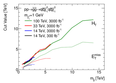
Figure 9 provides a comparison of the optimal cut at the different colliders that results from applying the analysis discussed in Sec. 3.2 as a function of gluino mass (assuming a 111 GeV neutralino). It is interesting to note that the slope of the HTsubscript𝐻𝑇H_{T} cut is larger than that for the ETmisssuperscriptsubscript𝐸𝑇missE_{T}^{\mathrm{miss}} cut. The search is taking advantage of the tremendous energy that is imparted to jets when these heavy gluinos decay. Furthermore, it is also interesting that the HTsubscript𝐻𝑇H_{T} cuts track very closely between machines (until mass of the gluino becomes so heavy that a given collider can no longer produce them in appreciable quantities), while the ETmisssuperscriptsubscript𝐸𝑇missE_{T}^{\mathrm{miss}} cuts begin to flatten out for very high mass gluinos. This can be understood by inspecting the histograms provided in Figs. 2, 4, and 6. The signal and background distributions have different shapes for ETmisssuperscriptsubscript𝐸𝑇missE_{T}^{\mathrm{miss}}, while the HTsubscript𝐻𝑇H_{T} of signal and background tend to fall off with a similar slope in the tails. The cut on on HTsubscript𝐻𝑇H_{T} therefore simply scales with the gluino mass, while the optimization for ETmisssuperscriptsubscript𝐸𝑇missE_{T}^{\mathrm{miss}} is more subtle. Finally, it is worth noting that due to the increase of the ratio of tt¯𝑡¯𝑡t\,\overline{t} to V+limit-from𝑉V+jets events as s𝑠\sqrt{s} increases, it is likely worth exploring the addition of a veto on b𝑏b-tagged jets for the higher energy colliders.

It is clear from these results that all four collider scenarios can have tremendous impact on our understanding of the gluino-neutralino parameter space. The next sections are devoted to exploring various details related to these conclusions.
Refer to caption
Figure 9: The optimal HTsubscript𝐻𝑇H_{T} [solid] and ETmisssuperscriptsubscript𝐸𝑇missE_{T}^{\mathrm{miss}} [dashed] cuts for the gluino-neutralino model with light flavor decays as a function of gluino mass (assuming a 111 GeV neutralino) for the four collider scenarios studied here.

3.10 Comparing Optimization Strategies

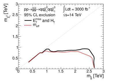
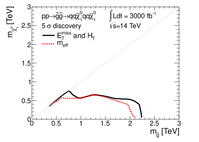
A two-dimensional optimization over cuts on ETmisssuperscriptsubscript𝐸𝑇missE_{T}^{\mathrm{miss}} and HTsubscript𝐻𝑇H_{T} is employed here. This is the most significant difference between our strategy and the cuts used in the ATLAS analysis [23], which only optimizes over meffHT+ETmisssubscript𝑚effsubscript𝐻𝑇superscriptsubscript𝐸𝑇missm_{\text{eff}}\equiv H_{T}+E_{T}^{\mathrm{miss}}. The purpose of this section is to quantify the gain in significance from performing the two-dimensional optimization. In Fig. 10, we plot the results of our mockup of the ATLAS one-dimensional scan along with the contours derived in this study by optimizing cuts over both ETmisssuperscriptsubscript𝐸𝑇missE_{T}^{\mathrm{miss}} and HTsubscript𝐻𝑇H_{T}. The two-dimensional strategy improves the reach for several regions of the signal grid. Therefore, we also use the two-dimensional strategy to study the squark-neutralino and gluino-squark signal models in the following sections.
Refer to caption
Refer to caption
Figure 10: The 5σ5𝜎5\sigma discovery contours [right] and expected 95%percent9595\% CL exclusion limits [left] for the one-dimensional meffsubscript𝑚effm_{\text{eff}} [red, dotted], and two-dimensional ETmisssuperscriptsubscript𝐸𝑇missE_{T}^{\mathrm{miss}} and HTsubscript𝐻𝑇H_{T} [black, solid] optimization strategies.
Refer to caption
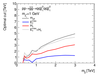
Figure 11: Optimal cuts on meffsubscript𝑚effm_{\text{eff}} [black, dotted], ETmisssuperscriptsubscript𝐸𝑇missE_{T}^{\mathrm{miss}} [blue, solid], and HTsubscript𝐻𝑇H_{T} [red, solid] for the 141414 TeV LHC with 3000 fb13000superscript fb13000\text{ fb}^{-1}. The mass of the neutralino is 1 GeV1 GeV1{\text{ GeV}}. Also plotted is ETmisssuperscriptsubscript𝐸𝑇missE_{T}^{\mathrm{miss}}+HTsubscript𝐻𝑇H_{T} [grey, solid] for the two-dimensional optimization, which allows direct comparison with meffsubscript𝑚effm_{\text{eff}} from the one-dimensional strategy.

It is interesting to compare the scaling of the optimal cut as a function of the gluino mass for the two optimization strategies. The optimal cuts which result for the meffsubscript𝑚effm_{\text{eff}} only [black, dotted] strategy along with the ETmisssuperscriptsubscript𝐸𝑇missE_{T}^{\mathrm{miss}} [blue, solid] and HTsubscript𝐻𝑇H_{T} [red, solid] are plotted in Fig. 11. Also shown is ETmiss+HTsuperscriptsubscript𝐸𝑇misssubscript𝐻𝑇E_{T}^{\mathrm{miss}}+H_{T} [grey, solid], which allows a direct comparison between the one-dimensional and two-dimensional optimizations. Above 1 TeVsimilar-toabsent1 TeV\sim 1{\text{ TeV}}, the cuts all increase monotonically as a function of mg~subscript𝑚~𝑔m_{\widetilde{g}}. The single cut on meffsubscript𝑚effm_{\text{eff}} tends to be harder than the sum of ETmisssuperscriptsubscript𝐸𝑇missE_{T}^{\mathrm{miss}} and HTsubscript𝐻𝑇H_{T}. The two-dimensional optimization can cover a wider parameter space of cuts, which allows it to take advantage of more complete information about the shape of the distribution. This allows it to perform as well or better with a slightly softer effective meffsubscript𝑚effm_{\text{eff}} cut.

3.11 Impact of Systematic Uncertainties

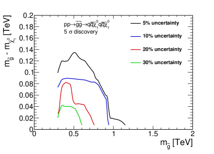
A systematic uncertainty of 20% was assumed for the background normalization in the results we have presented. It is likely that the experiments will significantly reduce these uncertainties with larger datasets and an improved understanding of their detectors; it is also possible that this value is aggressive given our current knowledge (or lack thereof) of physics at higher s𝑠\sqrt{s}. It is therefore interesting to understand the impact of different systematic uncertainties on the discovery reach.

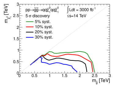
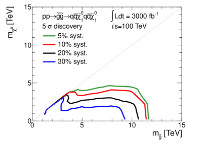
Figure 12 shows the impact from a change in the systematic uncertainty for gluino discovery at 14 TeV14 TeV14{\text{ TeV}} and 100 TeV100 TeV100{\text{ TeV}} with 300030003000fb-1. Varying the systematic background uncertainty from 30% to 5%, the discovery reach increases by roughly 600 GeV600 GeV600{\text{ GeV}} (3.4 TeV3.4 TeV3.4{\text{ TeV}}) in mg~subscript𝑚~𝑔m_{\widetilde{g}} at 14 TeV14 TeV14{\text{ TeV}} (100 TeV100 TeV100{\text{ TeV}}) and the coverage in mχ~10subscript𝑚superscriptsubscript~𝜒10m_{\widetilde{\chi}_{1}^{0}} direction is roughly doubled. The impact of systematic uncertainties on the 95%percent9595\% exclusion limits is less dramatic. Note that in this analysis we reoptimized the ETmisssuperscriptsubscript𝐸𝑇missE_{T}^{\mathrm{miss}} and HTsubscript𝐻𝑇H_{T} cuts for each choice of systematic uncertainty. As the LHC continues to run, the improvements in our understanding of the relevant backgrounds will be useful in extending the physics potential of the machine.
Refer to caption
Refer to caption
Figure 12: Expected 5σ5𝜎5\sigma discovery contours for the s=14𝑠14\sqrt{s}=14 TeV LHC [left] and a 100100100 TeV proton collider [right] with 300030003000 fb-1. The different curves correspond to various assumptions for the systematic uncertainty on the background: 5%percent55\% [green], 10%percent1010\% [red], 20%percent2020\% [blue], and 30%percent3030\% [black].

3.12 Impact of Pileup

In order to reach an integrated luminosity of 3000 fb13000superscript fb13000\text{ fb}^{-1}, the instantaneous luminosity at the LHC will need to increase significantly with respect to previous runs. There will be a corresponding increase in the number of pile-up events per bunch crossing. It is crucial to understand the impact this environment will have on the expected reach using this data set.

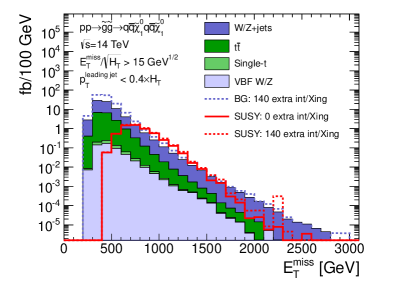
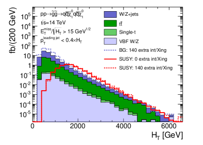
To study this in detail, we repeated the full analysis with signal and background samples that include 140 additional minimum-bias interactions. The Delphes based Snowmass simulation includes a pileup suppression algorithm that primarily impacts the ETmisssuperscriptsubscript𝐸𝑇missE_{T}^{\mathrm{miss}} resolution [9]. Figure 13 shows the ETmisssuperscriptsubscript𝐸𝑇missE_{T}^{\mathrm{miss}} [left] and HTsubscript𝐻𝑇H_{T} [right] distributions with and without pileup. The samples with pileup follow the distributions without pileup closely, especially in the search regions. We also observe that the the largest effects of pileup is at at low values of ETmisssuperscriptsubscript𝐸𝑇missE_{T}^{\mathrm{miss}}-significance, and are therefore suppressed by the requirement that ETmiss/HT>15 GeV1/2superscriptsubscript𝐸𝑇misssubscript𝐻𝑇15superscript GeV12E_{T}^{\mathrm{miss}}/\sqrt{H_{T}}>15\text{ GeV}^{1/2}.

The impact of pileup on the discovery significance [left] and limits [right] are shown in Fig. 14. Given that the HTsubscript𝐻𝑇H_{T} and ETmisssuperscriptsubscript𝐸𝑇missE_{T}^{\mathrm{miss}} distributions are effectively unchanged, it is not surprising that the results are very similar with and without pileup. The contours with and without pileup each lie within the other’s 1σ𝜎\sigma confidence interval, and we find no evidence that this reflects anything other than statistical fluctuations for a few signal points. We can safely assume that pileup has a small impact on this analysis.
Refer to caption
Refer to caption
Figure 13: Signal and background ETmisssuperscriptsubscript𝐸𝑇missE_{T}^{\mathrm{miss}} [left] and HTsubscript𝐻𝑇H_{T} [right] distributions at the 141414 TeV LHC for events with no pileup [solid] and the sum of backgrounds for events with 140 additional pp𝑝𝑝pp interactions per bunch crossing [dashed]. Additional interactions increase the background rates at low ETmisssuperscriptsubscript𝐸𝑇missE_{T}^{\mathrm{miss}}, but have little impact on the final analysis due to the tight ETmisssuperscriptsubscript𝐸𝑇missE_{T}^{\mathrm{miss}} cuts.
Refer to caption
Refer to caption
Figure 14: Discovery contours [right] and expected limits [left] for the analyses performed with [red, dotted] and without [black, solid] pileup at the 141414 TeV LHC with 3000 fb13000superscript fb13000\text{ fb}^{-1} integrated luminosity.

4 The Compressed Gluino-Neutralino Model with Light Flavor Decays

This section is devoted to analyses which target the compressed region of parameter space for the gluino-neutralino with light-flavor decays Simplified Model discussed in Sec. 3, where

mg~mχ~10Δmmg~.subscript𝑚~𝑔subscript𝑚superscriptsubscript~𝜒10Δ𝑚much-less-thansubscript𝑚~𝑔m_{\widetilde{g}}-m_{\widetilde{\chi}_{1}^{0}}\equiv\Delta m\ll m_{\widetilde{g}}. (1)

For models with this spectrum, the search strategy of Sec. 3 does not provide the optimal reach. With compressed spectra the gluino decays only generate soft partons, thereby suppressing the HTsubscript𝐻𝑇H_{T} signals and reducing the efficiency for passing the 444 jet requirement. A more effective strategy for compressed spectra searches relies instead on events with hard initial state radiation (ISR) jets to discriminate signal from background.

In this study, we will apply two different search strategies that are optimized for this kinematic configuration and will choose the one which leads to the most stringent bound on the production cross section for each point in parameter space. Some of the cuts chosen below are inspired by recent public results from ATLAS [31] and CMS [32] on monojet searches. For recent work on the compressed region of parameter space see [33], and for a discussion of the theoretical uncertainties see [34].

4.1 Dominant Backgrounds

The dominant background is the production of a Z𝑍Z boson in association with jets, where the Z𝑍Z boson decays into a pair of neutrinos (Zνν𝑍𝜈𝜈Z\rightarrow\nu\nu), leading to events with jets and a significant amount of missing transverse energy. Subleading backgrounds are the production of a W𝑊W boson which decays leptonically (Wν)𝑊𝜈\big{(}W\rightarrow\ell\,\nu\big{)} in association with jets, where the charged lepton is not reconstructed properly. Finally, when considering events with a significant number of jets, tt¯𝑡¯𝑡t\bar{t} production in the fully hadronic decay channel (tbqq)𝑡𝑏𝑞superscript𝑞\big{(}t\rightarrow b\,q\,q^{\prime}\big{)} can be relevant.

4.2   Two Analysis Strategies: 14 TeV

This section is devoted to a description of the two analysis strategies employed to search for the compressed regions of the gluino-neutralino parameter space. Applications to the 141414 TeV LHC will be presented for illustration; 333333 and 100100100 TeV will be discussed below. The following preselections are common to both approaches.

Preselection

  • lepton veto: any event with an electron or muon with pT>10subscript𝑝𝑇10p_{T}>10 GeV and |η|<2.5𝜂2.5|\eta|<2.5 is discarded

  • jets are required to have pT>30subscript𝑝𝑇30p_{T}>30 GeV and |η|<4.5𝜂4.5|\eta|<4.5

  • the leading jet must be reconstructed within |η|<2.5𝜂2.5|\eta|<2.5

  • ETmiss>100 GeVsuperscriptsubscript𝐸𝑇miss100 GeVE_{T}^{\mathrm{miss}}>100{\text{ GeV}}

The first set of cuts implemented in this analysis is based on the public monojet search from the ATLAS collaboration [31].

Search Strategy 1: Leading jet based selection

  • at most 2 jets

  • leading jet must have pT>(leading jet pT)optimalsubscript𝑝𝑇subscriptleading jet subscript𝑝𝑇optimalp_{T}>(\text{leading jet }p_{T})_{\text{optimal}} and |η|<2.0𝜂2.0|\eta|<2.0

  • second jet is allowed if Δφ(j2,ETmiss)>0.5Δ𝜑subscript𝑗2superscriptsubscript𝐸𝑇miss0.5\Delta\varphi(j_{2},E_{T}^{\mathrm{miss}})>0.5

  • ETmiss>(ETmiss)optimalsuperscriptsubscript𝐸𝑇misssubscriptsuperscriptsubscript𝐸𝑇missoptimalE_{T}^{\mathrm{miss}}>\big{(}E_{T}^{\mathrm{miss}}\big{)}_{\text{optimal}}

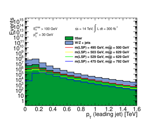
where both (ETmiss)optimalsubscriptsuperscriptsubscript𝐸𝑇missoptimal\big{(}E_{T}^{\mathrm{miss}}\big{)}_{\text{optimal}} and (leading jet pT)optimalsubscriptleading jet subscript𝑝𝑇optimal(\text{leading jet }p_{T})_{\text{optimal}} are determined simultaneously by taking the values in the range 1101101-10 TeV that yields the strongest exclusion. Figure 15 shows the distribution of the leading jet pTsubscript𝑝𝑇p_{T} and illustrates the ability to distinguish signal from background using this variable.
Refer to caption
Figure 15: Histogram of the leading jet pTsubscript𝑝𝑇p_{T} for signal and background at the 14 TeV14 TeV14{\text{ TeV}} LHC with 300 fb1300superscript fb1300\text{ fb}^{-1} after the preselection for a range of gluino and neutralino masses in the compressed region.

Table 4 shows the expected signal and background yields for the signal region with cuts on the leading jet pT>(500 GeV,1 TeV,2 TeV)subscript𝑝𝑇500 GeV1 TeV2 TeVp_{T}>(500{\text{ GeV}},1{\text{ TeV}},2{\text{ TeV}}) and ETmiss>(500 GeV,1 TeV,2 TeV)superscriptsubscript𝐸𝑇miss500 GeV1 TeV2 TeVE_{T}^{\mathrm{miss}}>(500{\text{ GeV}},1{\text{ TeV}},2{\text{ TeV}}) . This analysis is expected to be especially powerful for very small mass differences, when no jets except for a hard ISR jet can be reconstructed.

(mg~,mχ~10)subscript𝑚~𝑔subscript𝑚subscriptsuperscript~𝜒01\big{(}m_{\widetilde{g}},\,m_{\widetilde{\chi}^{0}_{1}}\big{)}\quad [GeV]
Cut V𝑉V+jets tt¯𝑡¯𝑡t\,\overline{t} Total BG (500, 495)500495(500,\,495) (792, 787)792787(792,\,787) (997, 992)997992(997,\,992)
Preselection 1.3×1091.3superscript1091.3\times 10^{9} 1.2×1081.2superscript1081.2\times 10^{8} 1.4×1091.4superscript1091.4\times 10^{9} 4.0×1074.0superscript1074.0\times 10^{7} 2.6×1062.6superscript1062.6\times 10^{6} 6.0×1056.0superscript1056.0\times 10^{5}
ETmiss>120superscriptsubscript𝐸𝑇miss120E_{T}^{\mathrm{miss}}>120 GeV, 2absent2\leq 2 jets 6.0×1086.0superscript1086.0\times 10^{8} 7.0×1067.0superscript1067.0\times 10^{6} 6.1×1086.1superscript1086.1\times 10^{8} 1.9×1071.9superscript1071.9\times 10^{7} 1.4×1061.4superscript1061.4\times 10^{6} 2.8×1052.8superscript1052.8\times 10^{5}
pT(j1)>120subscript𝑝𝑇subscript𝑗1120p_{T}(j_{1})>120 GeV, |η(j1)|<2.0𝜂subscript𝑗12.0|\eta(j_{1})|<2.0 3.2×1083.2superscript1083.2\times 10^{8} 3.2×1063.2superscript1063.2\times 10^{6} 3.6×1083.6superscript1083.6\times 10^{8} 1.2×1071.2superscript1071.2\times 10^{7} 9.2×1059.2superscript1059.2\times 10^{5} 1.9×1051.9superscript1051.9\times 10^{5}
Δφ(j2,ETmiss)>0.5Δ𝜑subscript𝑗2superscriptsubscript𝐸𝑇miss0.5\Delta{\varphi(j_{2},E_{T}^{\mathrm{miss}}})>0.5 2.4×1082.4superscript1082.4\times 10^{8} 1.6×1061.6superscript1061.6\times 10^{6} 2.4×1082.4superscript1082.4\times 10^{8} 8.0×1068.0superscript1068.0\times 10^{6} 6.4×1056.4superscript1056.4\times 10^{5} 1.3×1051.3superscript1051.3\times 10^{5}
ETmiss>500superscriptsubscript𝐸𝑇miss500E_{T}^{\mathrm{miss}}>500 GeV 4.5×1054.5superscript1054.5\times 10^{5} 1.7×1031.7superscript1031.7\times 10^{3} 4.5×1054.5superscript1054.5\times 10^{5} 4.5×1054.5superscript1054.5\times 10^{5} 5.9×1045.9superscript1045.9\times 10^{4} 1.6×1041.6superscript1041.6\times 10^{4}
pT(j1)>500subscript𝑝𝑇subscript𝑗1500p_{T}(j_{1})>500 GeV
ETmiss>1superscriptsubscript𝐸𝑇miss1E_{T}^{\mathrm{miss}}>1 TeV 9.4×1039.4superscript1039.4\times 10^{3} 131313 9.4×1039.4superscript1039.4\times 10^{3} 1.9×1041.9superscript1041.9\times 10^{4} 4.4×1034.4superscript1034.4\times 10^{3} 1.6×1031.6superscript1031.6\times 10^{3}
pT(j1)>1subscript𝑝𝑇subscript𝑗11p_{T}(j_{1})>1 TeV
ETmiss>2superscriptsubscript𝐸𝑇miss2E_{T}^{\mathrm{miss}}>2 TeV 494949 00 494949 878787 383838 181818
pT(j1)>2subscript𝑝𝑇subscript𝑗12p_{T}(j_{1})>2 TeV
Table 4: Number of expected events for s=14𝑠14\sqrt{s}=14 TeV and 300030003000 fb-1 for the background processes and three gluino-neutralino models in the compressed region. The leading jet pTsubscript𝑝𝑇p_{T} based selection with various cuts is applied. Three choices of cuts are provided for illustration.

Search Strategy 2: ETmisssuperscriptsubscript𝐸𝑇missE_{T}^{\mathrm{miss}} based selection without jet veto

  • leading jet with pT>110subscript𝑝𝑇110p_{T}>110 GeV and |η|<2.4𝜂2.4|\eta|<2.4

  • ETmiss>(ETmiss)optimalsuperscriptsubscript𝐸𝑇misssubscriptsuperscriptsubscript𝐸𝑇missoptimalE_{T}^{\mathrm{miss}}>(E_{T}^{\mathrm{miss}})_{\text{optimal}}

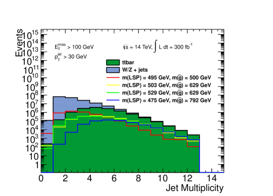
with ETmisssuperscriptsubscript𝐸𝑇missE_{T}^{\mathrm{miss}} varied in the range (1,10) TeV110 TeV(1,10){\text{ TeV}}. No requirement is placed on a maximum number of jets. Figure 16 shows that already for signal scenarios with small mass differences it is likely to reconstruct more than one jet in the event. Note that for higher jet multiplicities the production of top quark pairs in the fully hadronic decay mode starts to dominate over W/Z𝑊𝑍W/Z + jets production.

Refer to caption
Figure 16: Histogram of jet multiplicities for signal and background at the 14 TeV14 TeV14{\text{ TeV}} LHC with 300 fb1300superscript fb1300\text{ fb}^{-1} after the preselection for a range of gluino and neutralino masses in the compressed region.

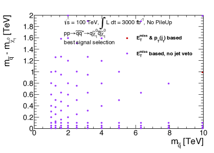
Table 5 shows the expected number of signal and background for three choices of the ETmisssuperscriptsubscript𝐸𝑇missE_{T}^{\mathrm{miss}} cut. Compared to the previous selection one can see that a significantly larger number of events are selected, especially for the larger mass differences. In addition, for this selection top pair production can make a non-negligible contribution to the total number of background events.

(mg~,mχ~10)subscript𝑚~𝑔subscript𝑚subscriptsuperscript~𝜒01\big{(}m_{\widetilde{g}},\,m_{\widetilde{\chi}^{0}_{1}}\big{)}\quad [GeV]
Cut V𝑉V+jets tt¯𝑡¯𝑡t\,\overline{t} Total BG (500, 495)500495(500,\,495) (792, 787)792787(792,\,787) (997, 992)997992(997,\,992)
Preselection 1.3×1091.3superscript1091.3\times 10^{9} 1.2×1081.2superscript1081.2\times 10^{8} 1.4×1091.4superscript1091.4\times 10^{9} 4.0×1074.0superscript1074.0\times 10^{7} 2.6×1062.6superscript1062.6\times 10^{6} 6.0×1056.0superscript1056.0\times 10^{5}
pT(j1)>110subscript𝑝𝑇subscript𝑗1110p_{T}(j_{1})>110 GeV, |η(j1)|<2.4𝜂subscript𝑗12.4|\eta(j_{1})|<2.4 7.9×1087.9superscript1087.9\times 10^{8} 8.1×1078.1superscript1078.1\times 10^{7} 8.7×1088.7superscript1088.7\times 10^{8} 3.0×1073.0superscript1073.0\times 10^{7} 2.1×1062.1superscript1062.1\times 10^{6} 4.8×1054.8superscript1054.8\times 10^{5}
ETmiss>500superscriptsubscript𝐸𝑇miss500E_{T}^{\mathrm{miss}}>500 GeV 2.1×1062.1superscript1062.1\times 10^{6} 1.5×1051.5superscript1051.5\times 10^{5} 2.3×1062.3superscript1062.3\times 10^{6} 2.4×1062.4superscript1062.4\times 10^{6} 2.9×1052.9superscript1052.9\times 10^{5} 7.5×1047.5superscript1047.5\times 10^{4}
ETmiss>1superscriptsubscript𝐸𝑇miss1E_{T}^{\mathrm{miss}}>1 TeV 4.9×1044.9superscript1044.9\times 10^{4} 2.1×1032.1superscript1032.1\times 10^{3} 5.2×1045.2superscript1045.2\times 10^{4} 1.3×1051.3superscript1051.3\times 10^{5} 2.5×1042.5superscript1042.5\times 10^{4} 8.1×1038.1superscript1038.1\times 10^{3}
ETmiss>2superscriptsubscript𝐸𝑇miss2E_{T}^{\mathrm{miss}}>2 TeV 278278278 333 282282282 900900900 328328328 133133133
Table 5: Number of expected events for s=14𝑠14\sqrt{s}=14 TeV and 300030003000 fb-1 for the background processes and selected signal processes. The selection without a veto on additional jets with cuts on ETmisssuperscriptsubscript𝐸𝑇missE_{T}^{\mathrm{miss}} is applied. Three choices of cuts are provided for illustration.

4.3   Results: 14 TeV

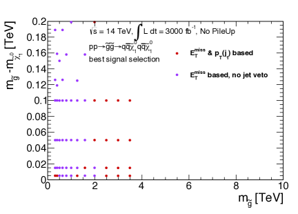
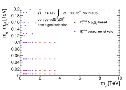
We now apply the compressed analysis to the gluino-neutralino model. Figure 17 shows which of the two selection strategies lead to the best discovery reach in the mχ~10 – mg~subscript𝑚superscriptsubscript~𝜒10 – subscript𝑚~𝑔m_{\widetilde{\chi}_{1}^{0}}\text{ -- }m_{\widetilde{g}} plane. For lighter gluinos and very small values of ΔmΔ𝑚\Delta m the leading jet based search dominates, while for higher masses and less compression the more inclusive ETmisssuperscriptsubscript𝐸𝑇missE_{T}^{\mathrm{miss}} based search leads to the strongest exclusion. Note that for the points with mg~2 TeVgreater-than-or-equivalent-tosubscript𝑚~𝑔2 TeVm_{\widetilde{g}}\gtrsim 2{\text{ TeV}} neither analysis can exclude the model so that the choice is not particularly relevant.
Refer to caption
Refer to caption
Figure 17: The choice of analysis that lead to the best discovery reach for a given point in parameter space for an integrated luminosity of 300300300 fb-1 [left] and 300030003000 fb-1 [right] at the 141414 TeV LHC for the compressed region of the gluino-neutralino Simplified Model with light flavor decays. The colors refer to the analyses as presented above: red circle = leading jet based, purple circle = ETmisssuperscriptsubscript𝐸𝑇missE_{T}^{\mathrm{miss}}-based. For very high gluino masses, neither analysis can exclude the signal process.

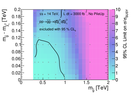
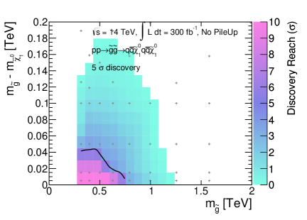
The results for integrated luminosities of 300300300 fb-1 and 300030003000 fb-1 at the 14 TeV14 TeV14{\text{ TeV}} LHC are shown in Fig. 18. A 20%percent2020\% systematic uncertainty is applied to the backgrounds. The assumed signal systematic are outlined in the appendix. Pile-up is neglected for these results; its impact is explored in Sec. 4.10 below.

With 300300300 fb-1 of data this search can exclude gluino masses of up to approximately 900900900 GeV for a mass difference of 555 GeV, with reduced reach for larger mass differences. The limits increase to around 111 TeV with a factor of 101010 more data. This improves the reach near the degenerate limit by roughly 200 GeV200 GeV200{\text{ GeV}} compared to the HTsubscript𝐻𝑇H_{T}-based analysis described in Sec. 3; the HTsubscript𝐻𝑇H_{T}-based searches do not begin to set stronger limits until Δ50 GeVgreater-than-or-equivalent-toΔ50 GeV\Delta\gtrsim 50{\text{ GeV}}. The combined discovery reach is shown in the bottom row of Fig. 18. The discovery reach of this search is gluino masses up to 800 GeV near the degenerate limit. Unlike the exclusion reach, the discovery reach for this search is not a substantial improvement over the HTsubscript𝐻𝑇H_{T}-based analysis, even in the degenerate limit. This occurs because the signal efficiency using these searches is such that there are not enough events to reach 5σ5𝜎5\sigma confidence. Overall, it is clear that the 141414 TeV LHC can have profound implications for models with compressed spectra.
Refer to caption
Refer to caption
Refer to caption
Refer to caption
Figure 18: Results for the compressed gluino-neutralino model with light flavor decays at the 141414 TeV LHC are given in the mg~mχ~10subscript𝑚~𝑔subscript𝑚superscriptsubscript~𝜒10m_{\widetilde{g}}-m_{\widetilde{\chi}_{1}^{0}} versus mg~subscript𝑚~𝑔m_{\widetilde{g}} plane. The top [bottom] row shows the expected 5σ5𝜎5\sigma discovery reach [95% confidence level upper limits] for gluino pair production. Mass points to the left/below the contours are expected to be probed at 300300300 fb-1 [left] and 300030003000 fb-1 [right]. A 20%percent2020\% systematic uncertainty is assumed for the background and pileup is not included.

4.4   Analysis: 33 TeV

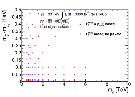
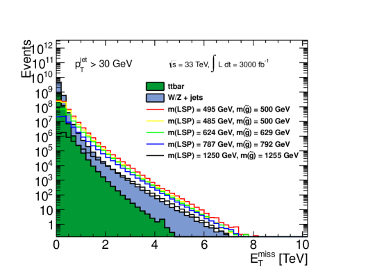
This section is devoted to the details of the 333333 TeV analysis in the compressed region of the gluino-neutralino model with light flavor decays. As the center-of-mass energy increases, the average pTsubscript𝑝𝑇p_{T} of an ISR jet would also increase. This implies that the probability for more than one ISR jets to pass the preselection cuts will be correspondingly higher, causing the ETmisssuperscriptsubscript𝐸𝑇missE_{T}^{\mathrm{miss}}-based search without additional jet veto to have the best acceptance of our search strategies. From Fig. 19, it is clear that this intuition holds; the ETmisssuperscriptsubscript𝐸𝑇missE_{T}^{\mathrm{miss}} based search gives the optimal significance for most of the parameter space studied here.

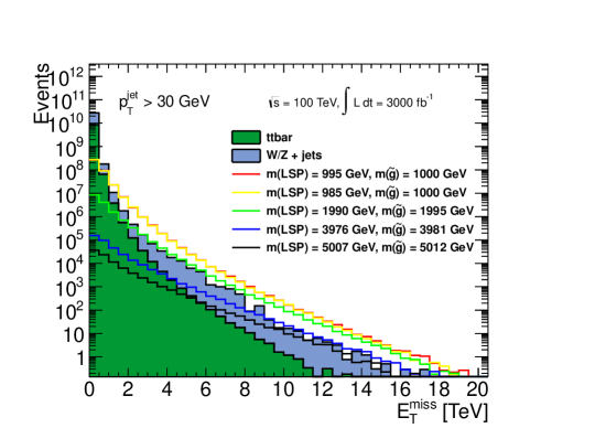
Figure 20 gives histograms of ETmisssuperscriptsubscript𝐸𝑇missE_{T}^{\mathrm{miss}} distribution for background and a variety of signal models. It is clear that a cut on ETmisssuperscriptsubscript𝐸𝑇missE_{T}^{\mathrm{miss}} can be used to distinguish signal from background. This can be seen quantitatively using Table 6, where the cut flows are given for background and three signal models.

Refer to caption
Figure 19: The choice of analysis that lead to the best discovery reach for a given point in parameter space for an integrated luminosity of 3000 fb-1 at a 333333 TeV proton collider for the compressed region of the gluino-neutralino Simplified Model with light flavor decays. The colors refer to the analyses as presented above: red circle = leading jet based, purple circle = ETmisssuperscriptsubscript𝐸𝑇missE_{T}^{\mathrm{miss}}-based. For very high gluino masses, neither analyses can exclude the signal process.
Refer to caption
Figure 20: Histogram of ETmisssuperscriptsubscript𝐸𝑇missE_{T}^{\mathrm{miss}} for signal and background at a 333333 TeV proton collider with 3000 fb13000superscript fb13000\text{ fb}^{-1} after the preselection for a range of gluino and neutralino masses in the compressed region.
(mg~,mχ~10)subscript𝑚~𝑔subscript𝑚subscriptsuperscript~𝜒01\big{(}m_{\widetilde{g}},\,m_{\widetilde{\chi}^{0}_{1}}\big{)}\quad [GeV]
Cut V𝑉V+jets tt¯𝑡¯𝑡t\,\overline{t} Total BG (797, 792)797792(797,\,792) (997, 992)997992(997,\,992) (1580, 1575)15801575(1580,\,1575)
Preselection 4.2×1094.2superscript1094.2\times 10^{9} 8.6×1088.6superscript1088.6\times 10^{8} 5.1×1095.1superscript1095.1\times 10^{9} 5.5×1075.5superscript1075.5\times 10^{7} 1.7×1071.7superscript1071.7\times 10^{7} 1.2×1061.2superscript1061.2\times 10^{6}
pTleadjet>110 GeV,|ηleadjet|<2.4formulae-sequencesuperscriptsubscript𝑝𝑇leadjet110 GeVsuperscript𝜂leadjet2.4p_{T}^{\text{leadjet}}>110\text{ GeV},|\eta^{\text{leadjet}}|<2.4 2.6×1092.6superscript1092.6\times 10^{9} 6.5×1086.5superscript1086.5\times 10^{8} 3.3×1093.3superscript1093.3\times 10^{9} 4.8×1074.8superscript1074.8\times 10^{7} 1.5×1071.5superscript1071.5\times 10^{7} 1.1×1061.1superscript1061.1\times 10^{6}
ETmiss>1 TeVsuperscriptsubscript𝐸𝑇miss1 TeVE_{T}^{\mathrm{miss}}>1\text{ TeV} 7.5×1057.5superscript1057.5\times 10^{5} 1.1×1051.1superscript1051.1\times 10^{5} 8.6×1058.6superscript1058.6\times 10^{5} 1.8×1061.8superscript1061.8\times 10^{6} 8.0×1058.0superscript105\color[rgb]{0,0,0}8.0\times 10^{5} 1.0×1051.0superscript1051.0\times 10^{5}
ETmiss>3 TeVsuperscriptsubscript𝐸𝑇miss3 TeVE_{T}^{\mathrm{miss}}>3\text{ TeV} 1.5×1031.5superscript1031.5\times 10^{3} 62 1.5×1031.5superscript1031.5\times 10^{3} 6.1×1036.1superscript1036.1\times 10^{3} 4.0×1034.0superscript1034.0\times 10^{3} 1.1×1031.1superscript103\color[rgb]{0,0,0}1.1\times 10^{3}
ETmiss>5 TeVsuperscriptsubscript𝐸𝑇miss5 TeVE_{T}^{\mathrm{miss}}>5\text{ TeV} 191919 00 191919 626262 505050 191919
Table 6: Number of expected events for s=33𝑠33\sqrt{s}=33 TeV and 300030003000 fb-1 for the background processes and selected signal processes. The selection without a veto on additional jets with cuts on ETmisssuperscriptsubscript𝐸𝑇missE_{T}^{\mathrm{miss}} is applied. Three choices of cuts are provided for illustration.

4.5   Results: 33 TeV

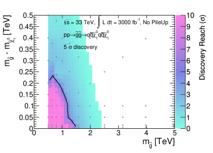
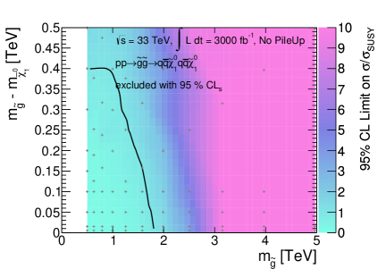
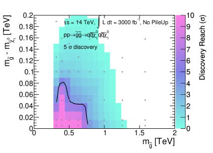
The 5σ5𝜎5\sigma discovery [left] and 95%percent9595\% C.L. limits [right] for the gluino-neutralino model are shown in Fig. 21, assuming 3000 fb13000superscript fb13000\text{ fb}^{-1} of integrated luminosity. 20%percent2020\% systematic uncertainty is applied to the backgrounds. The assumed signal systematic are outlined in the appendix. Pileup is not included; a demonstration that pileup will not significantly change these results is given in Sec. 4.10 below.

For a 333333 TeV proton collider with 300030003000 fb-1 of data, the exclusion reach for a mass difference of 555 GeV covers gluino masses of up to approximately 1.81.81.8 TeV, with reduced reach for larger mass differences. For very small mass differences in the range of 555 to 505050 GeV discoveries could be made for gluino masses up to 1.41.41.4 TeV. This search improves the exclusion (discovery) reach near the degenerate limit by roughly 800 GeV800 GeV800{\text{ GeV}} (400 GeV400 GeV400{\text{ GeV}}) compared to the HTsubscript𝐻𝑇H_{T}-based analysis described in Sec. 3; the HTsubscript𝐻𝑇H_{T}-based searches do not begin to set stronger limits until Δ50 GeVgreater-than-or-equivalent-toΔ50 GeV\Delta\gtrsim 50{\text{ GeV}}. Overall, it is clear that a 333333 TeV proton collider can have profound implications for models with compressed spectra.
Refer to caption
Refer to caption
Figure 21: Results for the compressed gluino-neutralino model with light flavor decays at a 333333 TeV proton collider with 3000 fb13000superscript fb13000\text{ fb}^{-1} are given in the mg~mχ~10subscript𝑚~𝑔subscript𝑚superscriptsubscript~𝜒10m_{\widetilde{g}}-m_{\widetilde{\chi}_{1}^{0}} versus mg~subscript𝑚~𝑔m_{\widetilde{g}} plane. The left [right] plot shows the expected 5σ5𝜎5\sigma discovery reach [95% confidence level upper limits] for gluino pair production. Mass points to the left/below the contours are expected to be probed at 300030003000 fb-1 [right]. A 20% systematic uncertainty is assumed for the background and pileup is not included.

4.6   Analysis: 100 TeV

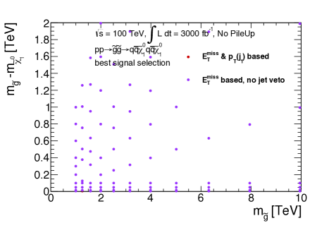
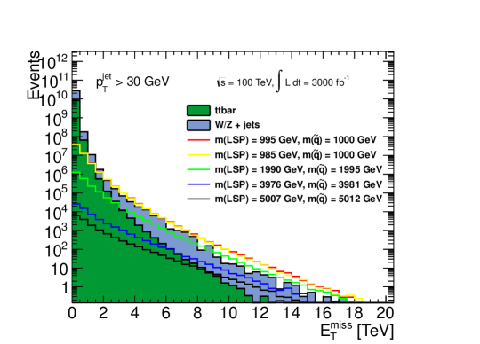
This section is devoted to the details of the 100100100 TeV analysis in the compressed region of the gluino-neutralino model with light flavor decays. As the center-of-mass energy increases, the average pTsubscript𝑝𝑇p_{T} of an ISR jet would also increase. This implies that the probability for more than one ISR jets to pass the preselection cuts will be correspondingly higher, causing the ETmisssuperscriptsubscript𝐸𝑇missE_{T}^{\mathrm{miss}}-based search to have the best acceptance of our search strategies. From Fig. 22, it is clear that this intuition holds; the ETmisssuperscriptsubscript𝐸𝑇missE_{T}^{\mathrm{miss}} based search gives the optimal significance for all of the probable parameter space. Figure 23 gives histograms of ETmisssuperscriptsubscript𝐸𝑇missE_{T}^{\mathrm{miss}} for background and a variety of signal models. It is clear that a cut on ETmisssuperscriptsubscript𝐸𝑇missE_{T}^{\mathrm{miss}} can be used to distinguish signal from background. This can be seen in Table 7 where the cut flows are given for background and three signal models.

Refer to caption
Figure 22: The choice of analysis that lead to the best discovery reach for a given point in parameter space for an integrated luminosity of 3000 fb-1 at a 100100100 TeV proton collider for the compressed region of the gluino-neutralino Simplified Model with light flavor decays. The colors refer to the analyses as presented above: red circle = leading jet based, purple circle = ETmisssuperscriptsubscript𝐸𝑇missE_{T}^{\mathrm{miss}}-based.
Refer to caption
Figure 23: Histogram of ETmisssuperscriptsubscript𝐸𝑇missE_{T}^{\mathrm{miss}} for signal and background at a 100100100 TeV proton collider with 3000 fb13000superscript fb13000\text{ fb}^{-1} after the preselection for a range of gluino and neutralino masses in the compressed region.
(mg~,mχ~10)subscript𝑚~𝑔subscript𝑚subscriptsuperscript~𝜒01\big{(}m_{\widetilde{g}},\,m_{\widetilde{\chi}^{0}_{1}}\big{)}\quad [GeV]
Cut V𝑉V+jets tt¯𝑡¯𝑡t\,\overline{t} Total BG (1995, 1990)19951990(1995,\,1990) (2512, 2507)25122507(2512,\,2507) (5012, 5007)50125007(5012,\,5007)
Preselection 1.7×10101.7superscript10101.7\times 10^{10} 7.0×1097.0superscript1097.0\times 10^{9} 2.4×10102.4superscript10102.4\times 10^{10} 1.3×1071.3superscript1071.3\times 10^{7} 4.1×1064.1superscript1064.1\times 10^{6} 7.9×1047.9superscript1047.9\times 10^{4}
pTleadjet>110 GeV,|ηleadjet|<2.4formulae-sequencesuperscriptsubscript𝑝𝑇leadjet110 GeVsuperscript𝜂leadjet2.4p_{T}^{\text{leadjet}}>110\text{ GeV},|\eta^{\text{leadjet}}|<2.4 1.2×10101.2superscript10101.2\times 10^{10} 6.1×1096.1superscript1096.1\times 10^{9} 1.9×10101.9superscript10101.9\times 10^{10} 1.3×1071.3superscript1071.3\times 10^{7} 4.1×1064.1superscript1064.1\times 10^{6} 7.9×1047.9superscript1047.9\times 10^{4}
ETmiss>3 TeVsuperscriptsubscript𝐸𝑇miss3 TeVE_{T}^{\mathrm{miss}}>3\text{ TeV} 1.3×1051.3superscript1051.3\times 10^{5} 2.0×1042.0superscript1042.0\times 10^{4} 1.5×1051.5superscript1051.5\times 10^{5} 1.9×1051.9superscript1051.9\times 10^{5} 9.4×1049.4superscript1049.4\times 10^{4} 4.8×1034.8superscript1034.8\times 10^{3}
ETmiss>6 TeVsuperscriptsubscript𝐸𝑇miss6 TeVE_{T}^{\mathrm{miss}}>6\text{ TeV} 3.6×1033.6superscript1033.6\times 10^{3} 229 3.8×1033.8superscript1033.8\times 10^{3} 8.0×1038.0superscript1038.0\times 10^{3} 5.1×1035.1superscript1035.1\times 10^{3} 509509509
ETmiss>9 TeVsuperscriptsubscript𝐸𝑇miss9 TeVE_{T}^{\mathrm{miss}}>9\text{ TeV} 100100100 999 109109109 612612612 410410410 676767
Table 7: Number of expected events for s=100𝑠100\sqrt{s}=100 TeV and 300030003000 fb-1 for the background processes and selected signal processes. The selection without a veto on additional jets with cuts on ETmisssuperscriptsubscript𝐸𝑇missE_{T}^{\mathrm{miss}} is applied. Three choices of cuts are provided for illustration.

4.7   Results: 100 TeV

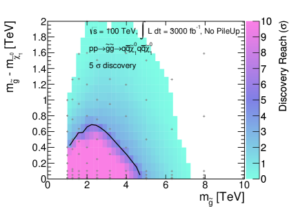
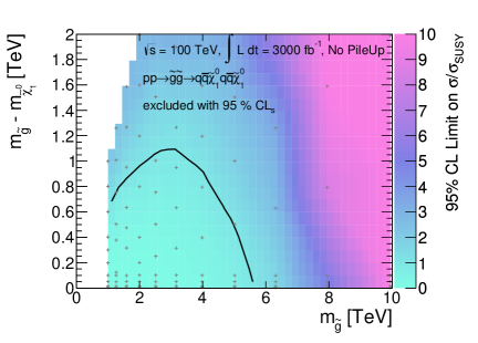
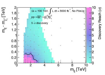
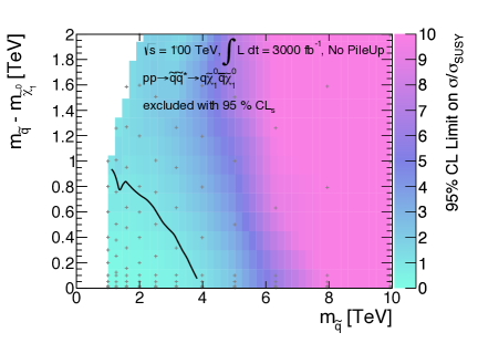
The 5σ5𝜎5\sigma discovery [left] and 95%percent9595\% C.L. limits [right] for the gluino-neutralino model are shown in Fig. 24, assuming 3000 fb13000superscript fb13000\text{ fb}^{-1} of integrated luminosity. 20%percent2020\% systematic uncertainty is applied to the backgrounds. The assumed signal systematic are outlined in the appendix. Pileup is not included; a demonstration that pileup will not significantly change these results is given in Sec. 4.10 below.

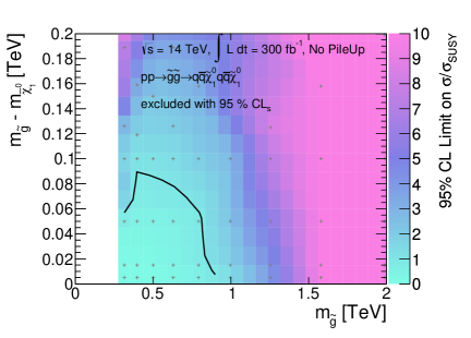
For a 100100100 TeV proton collider with 300030003000 fb-1 of data, the exclusion reach for a mass difference of 555 GeV covers gluino masses of up to approximately 5.75.75.7 TeV, with reduced reach for larger mass differences. For very small mass differences discoveries could be made for gluino masses up to 4.84.84.8 TeV. This search improves the exclusion (discovery) reach near the degenerate limit by roughly 1.7 TeV1.7 TeV1.7{\text{ TeV}} (1.3 TeV1.3 TeV1.3{\text{ TeV}}) compared to the HTsubscript𝐻𝑇H_{T}-based analysis described in Sec. 3; the HTsubscript𝐻𝑇H_{T}-based searches do not begin to set stronger limits until Δ500 GeVgreater-than-or-equivalent-toΔ500 GeV\Delta\gtrsim 500{\text{ GeV}}. Overall, it is clear that a 100100100 TeV proton collider can have profound implications for models with compressed spectra.
Refer to caption
Refer to caption
Figure 24: Results for the compressed gluino-neutralino model with light flavor decays at a 100100100 TeV proton collider are given in the mg~mχ~10subscript𝑚~𝑔subscript𝑚superscriptsubscript~𝜒10m_{\widetilde{g}}-m_{\widetilde{\chi}_{1}^{0}} versus mg~subscript𝑚~𝑔m_{\widetilde{g}} plane. The left [right] plot shows the expected 5σ5𝜎5\sigma discovery reach [95% confidence level upper limits] for gluino pair production. Mass points to the left/below the contours are expected to be probed at 300030003000 fb-1 [right]. A 20% systematic uncertainty is assumed for the background and pileup is not included.

4.8   Comparing Colliders

The search for the gluino-neutralino model with light flavor decays in the compressed region provides an interesting case study with which to compare the potential impact of different proton colliders. Figure 25 shows the 5σ5𝜎5\sigma discovery reach [95%percent9595\% CL exclusion] for two choices of integrated luminosity at 141414 TeV, along with the full data set assumed for 333333 and 100100100 TeV. At 141414 TeV, the factor of 101010 increase in luminosity leads to a modest increase from 900900900 GeV to 100010001000 GeV in the gluino limits. These limits have a strong dependence on the assumed systematic uncertainties. Therefore, the increase in luminosity does not have a tremendous impact on the ability to probe higher mass gluinos.

In contrast, increasing the center-of-mass energy has a tremendous impact on the experimentally available parameter space. For these machines, significantly heavier gluinos can be produced and more hard ISR jets are expected. For higher center-of-mass-energy, these searches specially targeted at the compressed region also become more and more important to fill in the gap in the reach of the untargeted search described in Sec. 3. Figure 25 makes a compelling case for investing in future proton colliders which can operate at these high energies.
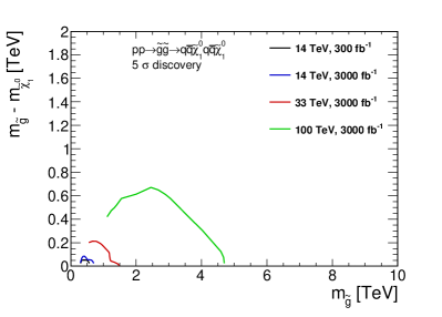
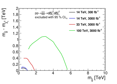
Refer to caption
Refer to caption
Figure 25: Results for the gluino-neutralino model with light flavor decays for the analyses that target the compressed region of parameter space. The left [right] panel shows the 5σ5𝜎5\,\sigma discovery reach [95%percent9595\% CL exclusion] for the four collider scenarios studied here. A 20%percent2020\% systematic uncertainty is assumed and pileup is not included.

4.9 Impact of Systematic Uncertainties

In the previous studies the systematic uncertainties on background are assumed to account for 20%percent2020\% on the overall background normalization. In the event of a discovery, it is likely that this error will be reduced dramatically as tremendous effort will be devoted to understanding these backgrounds in detail. It is therefore interesting to study the impact of this assumption.

Since the ETmisssuperscriptsubscript𝐸𝑇missE_{T}^{\mathrm{miss}}-based search is most relevant in the region where the 5σ5𝜎5\sigma contour lies (see Figs. 17 and 18), we demonstrate the impact of varying the systematic uncertainty for this search strategy for fixed cuts. The results for 3000 fb-1 of integrated luminosity at 14 TeV14 TeV14{\text{ TeV}} are shown in Fig. 26, where we fix ETmiss>2 TeVsuperscriptsubscript𝐸𝑇miss2 TeVE_{T}^{\mathrm{miss}}>2{\text{ TeV}} and plot the 5σ5𝜎5\sigma discovery reach for 30%percent3030\% [green], 20%percent2020\% [red], 10%percent1010\% [blue], and 5%percent55\% [black]. We see that a model with a degenerate gluino and neutralino could be discovered up to 600similar-toabsent600\sim 600 GeV (1.1 TeVsimilar-toabsent1.1 TeV\sim 1.1{\text{ TeV}}) for 30%percent3030\% (5%percent55\%) systematic uncertainty. The leading jet based search also has a comparable sensitivity to systematic uncertainties. Improving our understanding of the background, which could be in principle achieved by studying this large data set carefully, could improve the gluino reach by more than 400 GeV400 GeV400{\text{ GeV}}.

Refer to caption
Figure 26: Expected 5σ5𝜎5\sigma discovery contours for the s=14𝑠14\sqrt{s}=14 TeV LHC with 300030003000 fb-1 using the ETmisssuperscriptsubscript𝐸𝑇missE_{T}^{\mathrm{miss}} search strategy using a fixed cut of ETmiss>2 TeVsuperscriptsubscript𝐸𝑇miss2 TeVE_{T}^{\mathrm{miss}}>2{\text{ TeV}}. The different curves correspond to various assumptions for the systematic uncertainty on the background: 30%percent3030\% [green], 20%percent2020\% [red], 10%percent1010\% [blue], and 5%percent55\% [black].

4.10 Impact of Pileup

This section is devoted to an investigation of how the results for compressed spectra presented above would be affected by the presence of pileup. As discussed in Sec. 4.9, the strategy which yields the highest significance in the region where the 5σ5𝜎5\sigma contour lies is the ETmisssuperscriptsubscript𝐸𝑇missE_{T}^{\mathrm{miss}}-based search. Therefore, we use this search to demonstrate the impact of different pileup conditions.

Figure 27 gives the 5σ5𝜎5\sigma discovery contour [95%percent9595\% CL exclusion] on the left [right] for no pileup [black], 50 average events per bunch crossing [blue], and 140 average events per bunch crossing [red]. Surprisingly, we see that including pileup appears to increase the reach of this search. One possibility the search is picking up more otherwise “invisible” final states with soft ISR that become visible because there are pileup jets to push these events above the cut thresholds. In other words, this apparent improvement is due to the fact that we have a fixed grid of cuts for our optimization scans. Note that the limits for mg~mχ10~similar-to-or-equalssubscript𝑚~𝑔subscript𝑚~superscriptsubscript𝜒10m_{\widetilde{g}}\simeq m_{\widetilde{\chi_{1}^{0}}} remain unchanged; the presence of pileup only impacts somewhat larger mass differences.

Note that all the curves in Fig. 27 are computed for a fixed set of cuts, instead of reoptimizing for each pileup scenario which would obscure the comparison of the different limits. It is clear that including pileup only makes the reach stronger. The fact that we neglected pileup for the main results using these search strategies will imply that the limits we present are conservative.
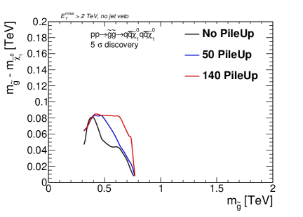
Refer to caption
Refer to caption
Figure 27: Expected 5σ5𝜎5\sigma discovery contours [left] and 95%percent9595\% CL limits [right] for the s=14𝑠14\sqrt{s}=14 TeV LHC with 300030003000 fb-1 using the ETmisssuperscriptsubscript𝐸𝑇missE_{T}^{\mathrm{miss}} search strategy for a fixed cut of ETmiss>2 TeVsuperscriptsubscript𝐸𝑇miss2 TeVE_{T}^{\mathrm{miss}}>2{\text{ TeV}}. The different curves correspond to the following average pileup: 00 [black], 505050 [blue], 140140140 [red].

5 The Squark-Neutralino Model

In the “squark-neutralino model”, the first and second generation squarks q~=u~L,u~R~𝑞subscript~𝑢𝐿subscript~𝑢𝑅\widetilde{q}=\widetilde{u}_{L},\widetilde{u}_{R}, d~L,d~R,subscript~𝑑𝐿subscript~𝑑𝑅\widetilde{d}_{L},\widetilde{d}_{R}, c~L,c~R,subscript~𝑐𝐿subscript~𝑐𝑅\widetilde{c}_{L},\widetilde{c}_{R}, s~L,s~Rsubscript~𝑠𝐿subscript~𝑠𝑅\widetilde{s}_{L},\widetilde{s}_{R} are the only kinematically accessible colored states. The gluino is completely decoupled from the squark production diagrams — the squark production cross section is significantly reduced compared to models where the gluino is just above the kinematic limit. The squarks decay directly to the LSP and the corresponding quark, q~iqiχ~10subscript~𝑞𝑖subscript𝑞𝑖superscriptsubscript~𝜒10\widetilde{q}_{i}\rightarrow q_{i}\,\widetilde{\chi}_{1}^{0}. The only two relevant parameters are the squark mass mq~subscript𝑚~𝑞m_{\widetilde{q}}, which is taken to be universal for the first two generations, and the neutralino mass mχ~10subscript𝑚superscriptsubscript~𝜒10m_{\widetilde{\chi}_{1}^{0}}. The model is summarized as:

BSM particles production decays
q~,χ~10~𝑞superscriptsubscript~𝜒10\widetilde{q},\,\widetilde{\chi}_{1}^{0} ppq~q~𝑝𝑝~𝑞superscript~𝑞p\,p\rightarrow\widetilde{q}\,\widetilde{q}^{*} q~qχ~10~𝑞𝑞subscriptsuperscript~𝜒01\widetilde{q}\rightarrow q\,\widetilde{\chi}^{0}_{1}

Due to the structure of the renormalization group equations in the Minimal SUSY SM, a heavy gluino would tend to raise the squark masses; some tuning is required to achieve light squarks. However, a class of theories with Dirac gluinos can be well approximated by this Simplified Model [35]. The current preliminary limits on this model using 202020 fb-1 of 888 TeV data are mq~=740 GeVsubscript𝑚~𝑞740 GeVm_{\widetilde{q}}=740\text{ GeV} (ATLAS [29]) and mq~=840 GeVsubscript𝑚~𝑞840 GeVm_{\widetilde{q}}=840\text{ GeV} (CMS [30]) assuming a massless neutralino.

Since the final state is two (or more) hard jets and missing energy, this model also serves to test the power of jets+ETmisssuperscriptsubscript𝐸𝑇missE_{T}^{\mathrm{miss}} style analyses. The mass reach is not be nearly as high as in the gluino-neutralino light flavor decay model for two reasons: neglecting ISR and FSR, the final state has only two hard jets from the squark decays as opposed to four hard jets from the gluino decays, and cross section for producing squark pairs with the gluino completely decoupled is substantially lower than that for producing gluino pairs of the same mass. Note that we checked that the 444 jet requirement included in the jets+ETmisssuperscriptsubscript𝐸𝑇missE_{T}^{\mathrm{miss}} preselection does not have a detrimental impact on the squark results presented below.

We simulated matched MadGraph samples for q~q~~𝑞superscript~𝑞\widetilde{q}\,\widetilde{q}^{*} with up to 2 additional generator level jets for the following points in parameter space:222We include 1 GeV1 GeV1{\text{ GeV}} for an example where the neutralino is effectively massless; the second line of neutralino masses is chosen to cover the bulk of the squark-neutralino plane; the final line is chosen to ensure coverage in the “compressed” region.

BSM particles masses
mq~subscript𝑚~𝑞m_{\widetilde{q}} [14 TeV]delimited-[]14 TeV\big{[}14{\text{ TeV}}\big{]} (315,397,500,629,792,997,1255,1580,1989,2489,2989) GeV31539750062979299712551580198924892989 GeV(315,397,500,629,792,997,1255,1580,1989,2489,2989){\text{ GeV}}
mq~subscript𝑚~𝑞m_{\widetilde{q}} [33 TeV]delimited-[]33 TeV\big{[}33{\text{ TeV}}\big{]} (500,629,792,997,1255,1580,1989,2489,2989,3489,(500,629,792,997,1255,1580,1989,2489,2989,3489,
3989,4489,4989,5489,5989) GeV3989,4489,4989,5489,5989){\text{ GeV}}
mq~subscript𝑚~𝑞m_{\widetilde{q}} [100 TeV]delimited-[]100 TeV\big{[}100{\text{ TeV}}\big{]} (1000,1259,1585,1995,2512,3162,3981,5012,6310,7944,(1000,1259,1585,1995,2512,3162,3981,5012,6310,7944,
9944,11944,13944,15944,17944,19944) GeV9944,11944,13944,15944,17944,19944){\text{ GeV}}
1 GeV1 GeV1{\text{ GeV}}
mχ~10subscript𝑚subscriptsuperscript~𝜒01m_{\widetilde{\chi}^{0}_{1}} (0.2,0.4,0.6,0.7,0.8,0.9)×mq~0.20.40.60.70.80.9subscript𝑚~𝑞(0.2,0.4,0.6,0.7,0.8,0.9)\times m_{\widetilde{q}}
mq~(100 GeV,50 GeV,15 GeV,5 GeV)subscript𝑚~𝑞100 GeV50 GeV15 GeV5 GeVm_{\widetilde{q}}-(100{\text{ GeV}},50{\text{ GeV}},15{\text{ GeV}},5{\text{ GeV}})

The signature of this model is multi-jets and ETmisssuperscriptsubscript𝐸𝑇missE_{T}^{\mathrm{miss}}. Therefore, the dominant backgrounds are identical to the ones relevant for the gluino-neutralino model with light flavor decays and are discussed in Sec 3.1. We use the same analysis strategy as for the gluino-neutralino model, described in Sec. 3.2, to project discovery reach and limits for this model. Given that pileup had no impact on the results using this search strategy as demonstrated in Sec. 3.12 above, we present here results only for the no pile-up scenario and expect little change when pileup is included.

Note that this search yields some power to discover these models in the difficult region of parameter space where the squark is degenerate with the neutralino, but Sec. 6 will provide the results of a search which is specifically targeted for this region of parameter space.

The next two sections give the details of the 141414 TeV LHC analysis and results.

5.1   Analysis: 14 TeV

Figure 28 shows the background and three signal distributions for the 141414 TeV LHC in the two kinematic variables which are scanned in this analysis: ETmisssuperscriptsubscript𝐸𝑇missE_{T}^{\mathrm{miss}} [left] and HTsubscript𝐻𝑇H_{T} [right]. In Table 8 we give the number of events after each stage of cuts for the dominant backgrounds and two signal models. From this table, it is clear that the 141414 TeV LHC with 3000 fb13000superscript fb13000\text{ fb}^{-1} would be able to exclude (but not discover) squarks with mass of 1255 GeV1255 GeV1255{\text{ GeV}}.

Refer to caption
Refer to caption
Figure 28: Histogram of ETmisssuperscriptsubscript𝐸𝑇missE_{T}^{\mathrm{miss}} [left] and HTsubscript𝐻𝑇H_{T} [right] after preselection cuts for background and a range of squark-neutralino models at the 141414 TeV LHC. The neutralino mass is 1 GeV1 GeV1{\text{ GeV}} for all signal models.
mq~subscript𝑚~𝑞\quad m_{\widetilde{q}}\quad [GeV]
Cut V𝑉V+jets tt¯𝑡¯𝑡t\bar{t} Total BG 500 1255
Preselection 2.07×1072.07superscript1072.07\times 10^{7} 2.47×1072.47superscript1072.47\times 10^{7} 4.54×1074.54superscript1074.54\times 10^{7} 2.94×1062.94superscript1062.94\times 10^{6} 1.41×1041.41superscript1041.41\times 10^{4}
ETmiss/HT>15 GeV1/2superscriptsubscript𝐸𝑇misssubscript𝐻𝑇15superscript GeV12E_{T}^{\mathrm{miss}}/\sqrt{H_{T}}>15\text{ GeV}^{1/2} 4.45×1054.45superscript1054.45\times 10^{5} 1.20×1051.20superscript1051.20\times 10^{5} 5.65×1055.65superscript1055.65\times 10^{5} 6.31×1056.31superscript1056.31\times 10^{5} 8.48×1038.48superscript1038.48\times 10^{3}
pTleading<0.4×HTsuperscriptsubscript𝑝𝑇leading0.4subscript𝐻𝑇p_{T}^{\mathrm{leading}}<0.4\times H_{T} 1.69×1051.69superscript1051.69\times 10^{5} 5.16×1045.16superscript1045.16\times 10^{4} 2.21×1052.21superscript1052.21\times 10^{5} 3.05×1053.05superscript1053.05\times 10^{5} 2.42×1032.42superscript1032.42\times 10^{3}
ETmiss>550superscriptsubscript𝐸𝑇miss550E_{T}^{\mathrm{miss}}>550 GeV 3.98×1043.98superscript1043.98\times 10^{4} 1.16×1041.16superscript1041.16\times 10^{4} 5.15×1045.15superscript1045.15\times 10^{4} 1.27×1051.27superscript1051.27\times 10^{5} 2.33×1032.33superscript1032.33\times 10^{3}
HT>600subscript𝐻𝑇600H_{T}>600 GeV
ETmiss>1200superscriptsubscript𝐸𝑇miss1200E_{T}^{\mathrm{miss}}>1200 GeV 174 23 197 185 222
HT>1400subscript𝐻𝑇1400H_{T}>1400 GeV
Table 8: Number of expected events for s=14𝑠14\sqrt{s}=14 TeV with 3000 fb-1 integrated luminosity for the background processes and selected squark masses for the squark-neutralino model. The neutralino mass is 1 GeV1 GeV1{\text{ GeV}}. Two choices of cuts on ETmisssuperscriptsubscript𝐸𝑇missE_{T}^{\mathrm{miss}} and HTsubscript𝐻𝑇H_{T} are provided, and for each squark mass column the entry in the row corresponding to the “optimal” cuts is marked in red.

5.2   Results: 14 TeV

The results for the squark-neutralino model are shown in Fig. 29 for the 141414 TeV LHC. The left [right] panels give discovery significance [95%percent9595\% CL exclusion] contours in the mχ~10subscript𝑚superscriptsubscript~𝜒10m_{\widetilde{\chi}_{1}^{0}} versus mq~subscript𝑚~𝑞m_{\widetilde{q}} plane. The top [bottom], results assume 300 fb1300superscript fb1300\text{ fb}^{-1} [3000 fb13000superscript fb13000\text{ fb}^{-1}] of data. As expected, the reach is significantly smaller than for the gluino-neutralino model with light flavor decays.

Using the NLO squark pair production cross section one can make a very naive estimate for the reach of a given collider. For example, we find that the choice of squark mass which would yield 101010 events at 300 fb1300superscript fb1300\text{ fb}^{-1} (3000 fb1)3000superscript fb1\big{(}3000\text{ fb}^{-1}\big{)} is 2.4(2.9) TeV2.42.9 TeV2.4\,(2.9){\text{ TeV}}. This roughly corresponds to the maximal possible reach one could expect for a given luminosity using 14 TeV14 TeV14{\text{ TeV}} proton collisions.

Using a realistic simulation framework along with the search strategy employed here the 14 TeV14 TeV14{\text{ TeV}} 300 fb1300superscript fb1300\text{ fb}^{-1} limit with massless neutralinos is projected to be 1.5 TeV1.5 TeV1.5{\text{ TeV}} (corresponding to 1022 events), while the 14 TeV14 TeV14{\text{ TeV}} 3000 fb13000superscript fb13000\text{ fb}^{-1} limit is projected to be 1.7 TeV1.7 TeV1.7{\text{ TeV}} (corresponding to 3482 events). Given these huge numbers of events, it is possible that a different (or more sophisticated) search strategy would allow for greater sensitivity to these models — this is outside the purview of the current study. Finally, we note that the 14 TeV14 TeV14{\text{ TeV}} LHC with 3000 fb13000superscript fb13000\text{ fb}^{-1} could discover a squark as heavy as 800 GeV800 GeV800{\text{ GeV}} if the neutralino is massless. Unlike in the gluino-neutralino model, the squark mass discovery reach immediately begins to weaken significantly as soon as the neutralino mass is increased from the massless limit.
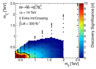
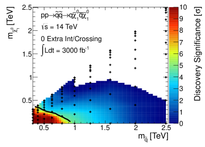
Refer to caption
Refer to caption
Refer to caption
Refer to caption
Figure 29: Results for the squark-neutralino model with light flavor decays are given in the mχ~10subscript𝑚superscriptsubscript~𝜒10m_{\widetilde{\chi}_{1}^{0}} versus mq~subscript𝑚~𝑞m_{\widetilde{q}} plane. The top [bottom] row shows the expected 5σ5𝜎5\sigma discovery reach [95%percent9595\% confidence level upper limits] for squark-anti-squark production at the 141414 TeV LHC. Mass points to the left/below the contours are expected to be probed with 300300300 fb-1 [left] and 300030003000 fb-1 [right] of data. A 20%percent2020\% systematic uncertainty is assumed for the backgrounds. Pileup is not included.

5.3   Analysis: 33 TeV

Figure 30 shows the background and three signal distributions for a 333333 TeV proton collider in the two kinematic variables which are scanned in this analysis: ETmisssuperscriptsubscript𝐸𝑇missE_{T}^{\mathrm{miss}} [left] and HTsubscript𝐻𝑇H_{T} [right]. In Table 9 we give the number of events after each stage of cuts for the dominant backgrounds and three signal models. From this table, it is clear that a 333333 TeV proton collider with 3000 fb13000superscript fb13000\text{ fb}^{-1} would be able to exclude (but not discover) squarks with mass of 3152 GeV3152 GeV3152{\text{ GeV}}.

Refer to caption
Refer to caption
Figure 30: Histogram of ETmisssuperscriptsubscript𝐸𝑇missE_{T}^{\mathrm{miss}} [left] and HTsubscript𝐻𝑇H_{T} [right] after preselection cuts for background and a range of squark-neutralino models at a 333333 TeV proton collider. The neutralino mass is 1 GeV1 GeV1{\text{ GeV}} for all signal models.
mq~subscript𝑚~𝑞m_{\tilde{q}} [GeV]
Cut V𝑉V+jets tt¯𝑡¯𝑡t\overline{t} Total BG 629629629 125512551255 315231523152
PreselectionPreselection\mathrm{Preselection} 1.55×1081.55superscript1081.55\times 10^{8} 2.86×1082.86superscript1082.86\times 10^{8} 4.42×1084.42superscript1084.42\times 10^{8} 1.20×1071.20superscript1071.20\times 10^{7} 3.99×1053.99superscript1053.99\times 10^{5} 926926926
ETmiss/HT>15 GeV1/2superscriptsubscript𝐸𝑇misssubscript𝐻𝑇15superscript GeV12E_{T}^{\mathrm{miss}}/\sqrt{H_{T}}>15{\text{ GeV}}^{1/2} 4.50×1064.50superscript1064.50\times 10^{6} 1.93×1061.93superscript1061.93\times 10^{6} 6.44×1066.44superscript1066.44\times 10^{6} 3.66×1063.66superscript1063.66\times 10^{6} 2.34×1052.34superscript1052.34\times 10^{5} 762
pTleading<0.4×HTsuperscriptsubscript𝑝𝑇leading0.4subscript𝐻𝑇p_{T}^{\mathrm{leading}}<0.4\times H_{T} 1.70×1061.70superscript1061.70\times 10^{6} 8.02×1058.02superscript1058.02\times 10^{5} 2.50×1062.50superscript1062.50\times 10^{6} 1.61×1061.61superscript1061.61\times 10^{6} 7.67×1047.67superscript1047.67\times 10^{4} 150150150
ETmiss>650 GeVsuperscriptsubscript𝐸𝑇miss650 GeVE_{T}^{\mathrm{miss}}>650{\text{ GeV}} 1.13×1061.13superscript1061.13\times 10^{6} 5.87×1055.87superscript1055.87\times 10^{5} 1.72×1061.72superscript1061.72\times 10^{6} 1.55×1061.55superscript1061.55\times 10^{6} 7.67×1047.67superscript1047.67\times 10^{4} 150150150
HT>650 GeVsubscript𝐻𝑇650 GeVH_{T}>650{\text{ GeV}}
ETmiss>1300 GeVsuperscriptsubscript𝐸𝑇miss1300 GeVE_{T}^{\mathrm{miss}}>1300{\text{ GeV}} 1.08×1041.08superscript1041.08\times 10^{4} 6.79×1036.79superscript1036.79\times 10^{3} 1.76×1041.76superscript1041.76\times 10^{4} 1.96×1041.96superscript1041.96\times 10^{4} 1.54×1041.54superscript1041.54\times 10^{4} 124124124
HT>1350 GeVsubscript𝐻𝑇1350 GeVH_{T}>1350{\text{ GeV}}
ETmiss>2650 GeVsuperscriptsubscript𝐸𝑇miss2650 GeVE_{T}^{\mathrm{miss}}>2650{\text{ GeV}} 51.551.551.5 16.316.316.3 67.867.867.8 50.850.850.8 26.926.926.9 22.322.322.3
HT>3350 GeVsubscript𝐻𝑇3350 GeVH_{T}>3350{\text{ GeV}}
Table 9: Number of expected events for s=33𝑠33\sqrt{s}=33 TeV with 3000 fb-1 integrated luminosity for the background processes and selected squark masses for the squark-neutralino model. The neutralino mass is 1 GeV1 GeV1{\text{ GeV}}. Three choices of cuts on ETmisssuperscriptsubscript𝐸𝑇missE_{T}^{\mathrm{miss}} and HTsubscript𝐻𝑇H_{T} are provided, and for each squark mass column the entry in the row corresponding to the “optimal” cuts is marked in red.

5.4   Results: 33 TeV

The results for the squark-neutralino model are shown in Fig. 31 for a 333333 TeV proton collider. Discovery significance [95%percent9595\% CL exclusion] contours in the mχ~10subscript𝑚superscriptsubscript~𝜒10m_{\widetilde{\chi}_{1}^{0}} versus mq~subscript𝑚~𝑞m_{\widetilde{q}} plane are shown on the left [right]. As expected, the reach is significantly smaller than for the gluino-neutralino model with light flavor decays.

Using the NLO squark pair production cross section one can make a very naive estimate for the reach of a given collider. For example, we find that the choice of squark mass which would yield 101010 events at 3000 fb13000superscript fb13000\text{ fb}^{-1} is 5.8 TeV5.8 TeV5.8{\text{ TeV}}. This roughly corresponds to the maximal possible reach one could expect for a given luminosity using 33 TeV33 TeV33{\text{ TeV}} proton collisions.

Using a realistic simulation framework along with the search strategy employed here the 33 TeV33 TeV33{\text{ TeV}} 3000 fb13000superscript fb13000\text{ fb}^{-1} limit with massless neutralinos is projected to be 3.4 TeV3.4 TeV3.4{\text{ TeV}} (corresponding to 3482 events). Given this huge number of events, it is possible that a different (or more sophisticated) search strategy would allow for greater sensitivity to these models — this is outside the purview of the current study. Finally, we note that the 33 TeV33 TeV33{\text{ TeV}} proton collider with 3000 fb13000superscript fb13000\text{ fb}^{-1} could discover a squark as heavy as 1.4 TeV1.4 TeV1.4{\text{ TeV}} if the neutralino is massless. As in the 141414 TeV search, the squark mass discovery reach immediately begins to weaken significantly as the neutralino mass is increased from the massless limit.
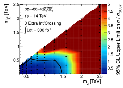
Refer to caption
Refer to caption
Figure 31: Results for the squark-neutralino model with light flavor decays are given in the mχ~10subscript𝑚superscriptsubscript~𝜒10m_{\widetilde{\chi}_{1}^{0}} versus mq~subscript𝑚~𝑞m_{\widetilde{q}} plane. The left [right] panels shows the expected 5σ5𝜎5\sigma discovery reach [95% confidence level upper limits] for squark-anti-squark production at a 333333 TeV proton collider. Mass points to the left/below the contours are expected to be probed with 300030003000 fb-1 of data [right]. A 20% systematic uncertainty is assumed for the backgrounds. Pileup is not included.

5.5   Analysis: 100 TeV

Figure 32 shows the background and three signal distributions for a 100100100 TeV proton collider in the two kinematic variables which are scanned in this analysis: ETmisssuperscriptsubscript𝐸𝑇missE_{T}^{\mathrm{miss}} [left] and HTsubscript𝐻𝑇H_{T} [right]. In Table 10 we give the number of events after each stage of cuts for the dominant backgrounds and a two signal models. From this table, it is clear that a 100100100 TeV proton collider with 3000 fb13000superscript fb13000\text{ fb}^{-1} would be able to exclude (but not discover) squarks with mass of 8 TeV8 TeV8{\text{ TeV}}.

Refer to caption
Refer to caption
Figure 32: Histogram of ETmisssuperscriptsubscript𝐸𝑇missE_{T}^{\mathrm{miss}} [left] and HTsubscript𝐻𝑇H_{T} [right] after preselection cuts for background and a range of squark-neutralino models at a 100100100 TeV proton collider. The neutralino mass is 1 GeV1 GeV1{\text{ GeV}} for all signal models.
mq~subscript𝑚~𝑞m_{\tilde{q}} [GeV]
Cut V𝑉V+jets tt¯𝑡¯𝑡t\overline{t} Total BG 316231623162 501250125012 794479447944
PreselectionPreselection\mathrm{Preselection} 1.64×1091.64superscript1091.64\times 10^{9} 3.33×1093.33superscript1093.33\times 10^{9} 4.97×1094.97superscript1094.97\times 10^{9} 2.01×1052.01superscript1052.01\times 10^{5} 1.44×1041.44superscript1041.44\times 10^{4} 668668668
ETmiss/HT>15 GeV1/2superscriptsubscript𝐸𝑇misssubscript𝐻𝑇15superscript GeV12E_{T}^{\mathrm{miss}}/\sqrt{H_{T}}>15{\text{ GeV}}^{1/2} 3.59×1073.59superscript1073.59\times 10^{7} 3.31×1073.31superscript1073.31\times 10^{7} 6.90×1076.90superscript1076.90\times 10^{7} 1.62×1051.62superscript1051.62\times 10^{5} 1.26×1041.26superscript1041.26\times 10^{4} 614614614
pTleading<0.4×HTsuperscriptsubscript𝑝𝑇leading0.4subscript𝐻𝑇p_{T}^{\mathrm{leading}}<0.4\times H_{T} 1.19×1071.19superscript1071.19\times 10^{7} 1.25×1071.25superscript1071.25\times 10^{7} 2.44×1072.44superscript1072.44\times 10^{7} 4.14×1044.14superscript1044.14\times 10^{4} 2.63×1032.63superscript1032.63\times 10^{3} 96.996.996.9
ETmiss>5550 GeVsuperscriptsubscript𝐸𝑇miss5550 GeVE_{T}^{\mathrm{miss}}>5550{\text{ GeV}} 242424 21.221.221.2 45.145.145.1 73.373.373.3 60.160.160.1 19.919.919.9
HT>900 GeVsubscript𝐻𝑇900 GeVH_{T}>900{\text{ GeV}}
ETmiss>4900 GeVsuperscriptsubscript𝐸𝑇miss4900 GeVE_{T}^{\mathrm{miss}}>4900{\text{ GeV}} 61.261.261.2 53.353.353.3 114114114 119119119 143143143 29.5
HT>5450 GeVsubscript𝐻𝑇5450 GeVH_{T}>5450{\text{ GeV}}
ETmiss>6150 GeVsuperscriptsubscript𝐸𝑇miss6150 GeVE_{T}^{\mathrm{miss}}>6150{\text{ GeV}} 9.29.29.2 8.48.48.4 17.617.617.6 11.211.211.2 171717 11.511.511.5
HT>8200 GeVsubscript𝐻𝑇8200 GeVH_{T}>8200{\text{ GeV}}
Table 10: Number of expected events for s=100𝑠100\sqrt{s}=100 TeV with 3000 fb-1 integrated luminosity for the background processes and selected squark masses for the squark-neutralino model. The neutralino mass is 1 GeV1 GeV1{\text{ GeV}}. Three choices of cuts on ETmisssuperscriptsubscript𝐸𝑇missE_{T}^{\mathrm{miss}} and HTsubscript𝐻𝑇H_{T} are provided, and for each squark mass column the entry in the row corresponding to the “optimal” cuts is marked in red.

5.6   Results: 100 TeV

The results for the squark-neutralino model are shown in Fig. 33 for a 100100100 TeV proton collider. Discovery significance [95%percent9595\% CL exclusion] contours in the mχ~10subscript𝑚superscriptsubscript~𝜒10m_{\widetilde{\chi}_{1}^{0}} versus mq~subscript𝑚~𝑞m_{\widetilde{q}} plane are shown on the left [right]. As expected, the reach is significantly smaller than for the gluino-neutralino model with light flavor decays.

Using the NLO gluino pair production cross section one can make a very naive estimate for the reach of a given collider. For example, we find that the choice of squark mass which would yield 101010 events at 3000 fb13000superscript fb13000\text{ fb}^{-1} is 14.8 TeV14.8 TeV14.8{\text{ TeV}}. This roughly corresponds to the maximal possible reach one could expect for a given luminosity using 100 TeV100 TeV100{\text{ TeV}} proton collisions.

Using a realistic simulation framework along with the search strategy employed here the 100 TeV100 TeV100{\text{ TeV}} 3000 fb13000superscript fb13000\text{ fb}^{-1} limit with massless neutralinos is projected to be 8.0 TeV8.0 TeV8.0{\text{ TeV}} (corresponding to 849 events). Given this huge number of events, it is possible that a different (or more sophisticated) search strategy would allow for greater sensitivity to these models — this is outside the purview of the current study. Finally, we note that the 100 TeV100 TeV100{\text{ TeV}} proton collider with 3000 fb13000superscript fb13000\text{ fb}^{-1} could discover a squark as heavy as 2.4 TeV2.4 TeV2.4{\text{ TeV}} if the neutralino is massless. Compared to the 141414 and 333333 TeV searches, the squark reach degrades less rapidly as the neutralino mass is increased from the massless limit. The next section provides a comparison of the impact that the four collider scenarios studied here can have on the parameter space of this model.
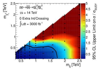
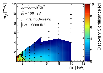
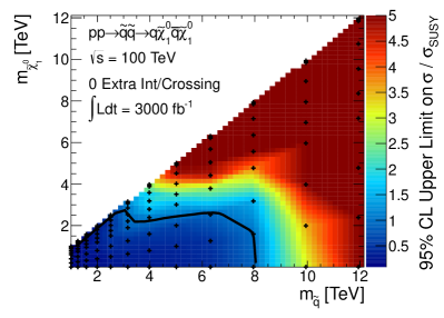
Refer to caption
Refer to caption
Figure 33: Results for the squark-neutralino model with light flavor decays are given in the mχ~10subscript𝑚superscriptsubscript~𝜒10m_{\widetilde{\chi}_{1}^{0}} versus mq~subscript𝑚~𝑞m_{\widetilde{q}} plane. The left [right] panels shows the expected 5σ5𝜎5\sigma discovery reach [95% confidence level upper limits] for squark-anti-squark production at a 100100100 TeV proton collider. Mass points to the left/below the contours are expected to be probed with 300030003000 fb-1 of data [right]. A 20% systematic uncertainty is assumed for the backgrounds. Pileup is not included.

5.7   Comparing Colliders

The squark-neutralino model has a similar multi-jet plus ETmisssuperscriptsubscript𝐸𝑇missE_{T}^{\mathrm{miss}} signature to the gluino-neutralino model with light flavor decays. However, the squark-neutralino model is more difficult to probe due to the smaller number of hard jets in the final state coupled with the substantially smaller production cross section. Since this model provides a more challenging scenario, it is interesting to understand the impact that can be made on exploring the parameter space with different collider scenarios. Figure 34 shows the 5σ5𝜎5\sigma discovery reach [95%percent9595\% CL exclusion] for two choices of integrated luminosity at 141414 TeV, along with the reach using the full data set assumed for 333333 and 100100100 TeV.

In general, we find that due to the small cross sections, it is very difficult to distinguish this model from background with discovery level significance333It is worth noting that this search, which was devised originally to target gluinos, has not been extensively optimized for the signature of squark pair production. It is possible that a search exactly tailored to this signal could improve the reach beyond what is found here.. Consequentially, the discovery reach does not appear to significantly improve with the 141414 TeV luminosity upgrade. The discovery reach in the massless neutralino limit also scales slowly with the CM energy, increasing only by a factor of 333 from 141414 TeV to 100100100 TeV, compared to a factor of 555 for the gluino-neutralino model.

The exclusion reach for the squark-neutralino models is much more favorable in comparison. At this level of significance the background systematics are less difficult to overcome, and the limits scale much more favorably with luminosity and CM energy, as in the gluino-neutralino model. Figure 8 makes a compelling case for investing in future proton colliders which can operate at these high energies.
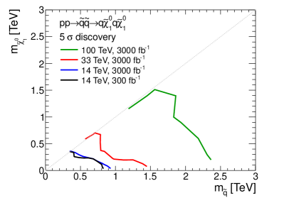
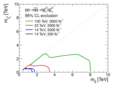
Refer to caption
Refer to caption
Figure 34: Results for the squark-neutralino model. The left [right] panel shows the 5σ5𝜎5\,\sigma discovery reach [95%percent9595\% CL exclusion] for the four collider scenarios studied here. A 20%percent2020\% systematic uncertainty is assumed and pileup is not included.

6 The Compressed Squark-Neutralino Model

The results presented in the previous section were derived using a search which targeted the bulk of the squark-neutralino Simplified Model parameter space. In the compressed region where

mq~mχ~10Δmmq~subscript𝑚~𝑞subscript𝑚superscriptsubscript~𝜒10Δ𝑚much-less-thansubscript𝑚~𝑞m_{\widetilde{q}}-m_{\widetilde{\chi}_{1}^{0}}\equiv\Delta m\ll m_{\widetilde{q}} (2)

a different search strategy is required. For parameters in this range, the jets which result from the direct decays of the squark will be very soft and one has to rely on ISR jets to discriminate these models from background. These signatures will be very similar to those produced by the compressed gluino-neutralino model with light flavor decays, and therefore the backgrounds will be identical to those described above in Sec. 4.1. Therefore, we will use the same search strategies described above in Sec. 4.

6.1   Analysis: 14 TeV

As can be seen in Fig 35, for the very small squark masses excludable in the compressed region the only relevant strategy is the ETmisssuperscriptsubscript𝐸𝑇missE_{T}^{\mathrm{miss}} based search. A histogram of the discriminating variable relevant for this search is shown in Fig. 36. We also give the number of events after cuts for this strategy in Table 11. It is clear that for low mass squarks, it is possible that the signal could be distinguished over background.
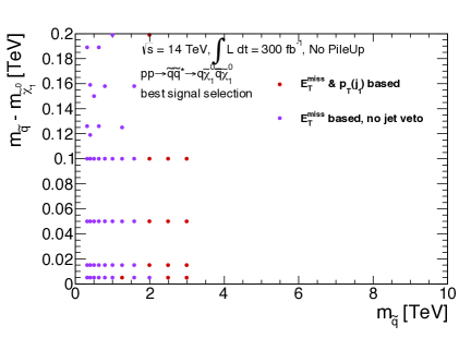
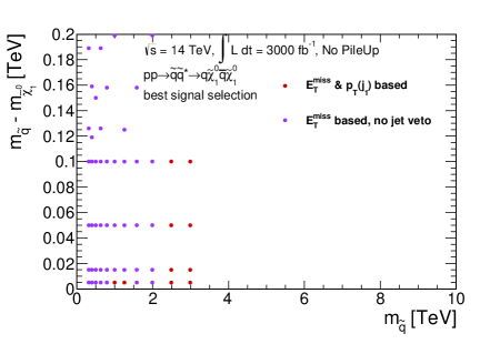
Refer to caption
Refer to caption
Figure 35: The choice of analysis strategy that leads to the best discovery reach for a given point in parameter space for an integrated luminosity of 300 fb-1 [left] and 3000 fb-1 [right] for the compressed region of the squark-neutralino model. The colors refer to the analyses as presented above: red circle = leading jet based, purple circle = ETmisssuperscriptsubscript𝐸𝑇missE_{T}^{\mathrm{miss}}-based.
Refer to caption
Figure 36: Histogram of ETmisssuperscriptsubscript𝐸𝑇missE_{T}^{\mathrm{miss}} for signal and background after the preselection for a range of squark and neutralino masses in the compressed region.
(mq~,mχ~10)subscript𝑚~𝑞subscript𝑚subscriptsuperscript~𝜒01\big{(}m_{\widetilde{q}},\,m_{\widetilde{\chi}^{0}_{1}}\big{)}\quad [GeV]
Cut V𝑉V+jets tt¯𝑡¯𝑡t\,\overline{t} Total BG (500, 495)500495(500,\,495) (792, 787)792787(792,\,787) (997, 992)997992(997,\,992)
Preselection 1.3×1091.3superscript1091.3\times 10^{9} 1.2×1081.2superscript1081.2\times 10^{8} 1.4×1091.4superscript1091.4\times 10^{9} 5.8×1065.8superscript1065.8\times 10^{6} 4.3×1054.3superscript1054.3\times 10^{5} 9.8×1049.8superscript1049.8\times 10^{4}
pTleadjet>110 GeV,|ηleadjet|<2.4formulae-sequencesuperscriptsubscript𝑝𝑇leadjet110 GeVsuperscript𝜂leadjet2.4p_{T}^{\text{leadjet}}>110\text{ GeV},|\eta^{\text{leadjet}}|<2.4 7.9×1087.9superscript1087.9\times 10^{8} 8.1×1078.1superscript1078.1\times 10^{7} 8.7×1088.7superscript1088.7\times 10^{8} 4.5×1064.5superscript1064.5\times 10^{6} 3.5×1053.5superscript1053.5\times 10^{5} 8.0×1048.0superscript1048.0\times 10^{4}
ETmiss>500 GeVsuperscriptsubscript𝐸𝑇miss500 GeVE_{T}^{\mathrm{miss}}>500\text{ GeV} 2.1×1062.1superscript1062.1\times 10^{6} 1.5×1051.5superscript1051.5\times 10^{5} 2.3×1062.3superscript1062.3\times 10^{6} 4.5×1054.5superscript1054.5\times 10^{5} 5.2×1045.2superscript1045.2\times 10^{4} 1.4×1041.4superscript1041.4\times 10^{4}
ETmiss>1 TeVsuperscriptsubscript𝐸𝑇miss1 TeVE_{T}^{\mathrm{miss}}>1\text{ TeV} 4.9×1044.9superscript1044.9\times 10^{4} 2.1×1032.1superscript1032.1\times 10^{3} 5.2×1045.2superscript1045.2\times 10^{4} 3.0×1043.0superscript1043.0\times 10^{4} 5.0×1035.0superscript1035.0\times 10^{3} 1.6×1031.6superscript1031.6\times 10^{3}
ETmiss>2 TeVsuperscriptsubscript𝐸𝑇miss2 TeVE_{T}^{\mathrm{miss}}>2\text{ TeV} 278278278 333 282282282 237237237 646464 242424
Table 11: Number of expected events for s=14𝑠14\sqrt{s}=14 TeV and 300030003000 fb-1 for the background processes and selected signal processes. The selection without a veto on additional jets with cuts on ETmisssuperscriptsubscript𝐸𝑇missE_{T}^{\mathrm{miss}} is applied. Three choices of cuts are provided for illustration.

6.2   Results: 14 TeV

The results for the squark neutralino model in the compressed region of parameter space are given in Fig. 37. As discussed above, only the ETmisssuperscriptsubscript𝐸𝑇missE_{T}^{\mathrm{miss}} based strategy (see Sec. 4) is relevant for this model at the 141414 TeV LHC. It is possible to exclude (discover) squarks in the degenerate limit with mass less than 650 GeV(500 GeV)similar-toabsent650 GeV500 GeV\sim 650{\text{ GeV}}(500{\text{ GeV}}) with 300 fb1300superscript fb1300\text{ fb}^{-1} of data. Increasing the integrated luminosity by a factor of 10 has a minimal impact on the discovery reach for compressed squark models. This search improves the exclusion (discovery) reach near the degenerate limit by roughly 300 GeV(150 GeV)300 GeV150 GeV300{\text{ GeV}}(150{\text{ GeV}}) compared to the HTsubscript𝐻𝑇H_{T}-based analysis described in Sec. 5; the HTsubscript𝐻𝑇H_{T}-based searches do not begin to set stronger limits until Δ50 GeVgreater-than-or-equivalent-toΔ50 GeV\Delta\gtrsim 50{\text{ GeV}}. Finally, we note that given our results for the compressed gluino-neutralino study in Sec. 4.10 above, pileup is not expected to have a significant impact on these conclusions. The compressed region of this model will be difficult to probe at the 14 TeV14 TeV14{\text{ TeV}} LHC, but will still represent a significant improvement over current bounds.

Refer to caption
Refer to caption
Refer to caption
Refer to caption
Figure 37: Results for the compressed squark-neutralino model with light flavor decays are given in the mq~mχ~10subscript𝑚~𝑞subscript𝑚superscriptsubscript~𝜒10m_{\widetilde{q}}-m_{\widetilde{\chi}_{1}^{0}} versus mq~subscript𝑚~𝑞m_{\widetilde{q}} plane. The top [bottom] row shows the expected 5σ5𝜎5\sigma discovery reach [95% confidence level upper limits] for squark-anti-squark production. Mass points to the left/below the contours are expected to be probed at 300 fb-1 [left] and 3000 fb-1 [right]. A 20% systematic uncertainty is assumed for the background. Pileup is not included.

6.3   Analysis: 33 TeV

As discussed above in the context of the compressed region of the gluino-neutralino model, the ETmisssuperscriptsubscript𝐸𝑇missE_{T}^{\mathrm{miss}} based search tends to be more powerful at the higher energy colliders since the probability of having multiple ISR jets increases. From Fig. 38, it is clear that the relevant strategy in the region that can be probed by this machine is the ETmisssuperscriptsubscript𝐸𝑇missE_{T}^{\mathrm{miss}} based search. A histogram of the discriminating variable relevant for this search is shown in Fig. 39. We also give the number of events after cuts for this strategy in Table 12. It is clear that for low mass squarks, it is possible that the signal could be distinguished over background.
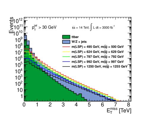
Refer to caption
Figure 38: The choice of analysis that lead to the best discovery reach for a given point in parameter space for an integrated luminosity of 3000 fb-1 at a 333333 TeV proton collider for the compressed region of the squark-neutralino Simplified Model with light flavor decays. The colors refer to the analyses as presented above: red circle = leading jet based, purple circle = ETmisssuperscriptsubscript𝐸𝑇missE_{T}^{\mathrm{miss}}-based.
Refer to caption
Figure 39: Histogram of ETmisssuperscriptsubscript𝐸𝑇missE_{T}^{\mathrm{miss}} for signal and background at a 333333 TeV proton collider after the preselection for a range of squark and neutralino masses in the compressed region.
(mq~,mχ~10)subscript𝑚~𝑞subscript𝑚subscriptsuperscript~𝜒01\big{(}m_{\widetilde{q}},\,m_{\widetilde{\chi}^{0}_{1}}\big{)}\quad [GeV]
Cut V𝑉V+jets tt¯𝑡¯𝑡t\,\overline{t} Total BG (797, 787)797787(797,\,787) (997, 992)997992(997,\,992) (1580, 1575)15801575(1580,\,1575)
Preselection 4.2×1094.2superscript1094.2\times 10^{9} 8.6×1088.6superscript1088.6\times 10^{8} 5.1×1095.1superscript1095.1\times 10^{9} 8.4×1068.4superscript1068.4\times 10^{6} 2.6×1062.6superscript1062.6\times 10^{6} 2.0×1052.0superscript1052.0\times 10^{5}
pTleadjet>110 GeV,|ηleadjet|<2.4formulae-sequencesuperscriptsubscript𝑝𝑇leadjet110 GeVsuperscript𝜂leadjet2.4p_{T}^{\text{leadjet}}>110\text{ GeV},|\eta^{\text{leadjet}}|<2.4 2.6×1092.6superscript1092.6\times 10^{9} 6.5×1086.5superscript1086.5\times 10^{8} 3.3×1093.3superscript1093.3\times 10^{9} 7.2×1067.2superscript1067.2\times 10^{6} 2.3×1062.3superscript1062.3\times 10^{6} 1.8×1051.8superscript1051.8\times 10^{5}
ETmiss>1 TeVsuperscriptsubscript𝐸𝑇miss1 TeVE_{T}^{\mathrm{miss}}>1\text{ TeV} 7.5×1057.5superscript1057.5\times 10^{5} 1.1×1051.1superscript1051.1\times 10^{5} 8.6×1058.6superscript1058.6\times 10^{5} 3.5×1053.5superscript1053.5\times 10^{5} 1.5×1051.5superscript105\color[rgb]{0,0,0}1.5\times 10^{5} 2.0×1042.0superscript1042.0\times 10^{4}
ETmiss>3 TeVsuperscriptsubscript𝐸𝑇miss3 TeVE_{T}^{\mathrm{miss}}>3\text{ TeV} 1.5×1031.5superscript1031.5\times 10^{3} 626262 1.5×1031.5superscript1031.5\times 10^{3} 2.1×1032.1superscript1032.1\times 10^{3} 1.3×1031.3superscript1031.3\times 10^{3} 315315315
ETmiss>5 TeVsuperscriptsubscript𝐸𝑇miss5 TeVE_{T}^{\mathrm{miss}}>5\text{ TeV} 191919 00 191919 303030 202020 777
Table 12: Number of expected events for s=33𝑠33\sqrt{s}=33 TeV and 300030003000 fb-1 for the background processes and selected signal processes. The selection without a veto on additional jets with cuts on ETmisssuperscriptsubscript𝐸𝑇missE_{T}^{\mathrm{miss}} is applied. Three choices of cuts are provided for illustration.

6.4   Results: 33 TeV

The results for the squark neutralino model in the compressed region of parameter space are given in Fig. 40. As discussed above, only the ETmisssuperscriptsubscript𝐸𝑇missE_{T}^{\mathrm{miss}} based strategy (see Sec. 4) is relevant for this model at a 333333 TeV proton collider. It is possible to exclude (discover) squarks in the degenerate limit with mass less than 1.2(0.7) TeVsimilar-toabsent1.20.7 TeV\sim 1.2(0.7){\text{ TeV}} with 3000 fb13000superscript fb13000\text{ fb}^{-1} of data. This does not substantially improves the discovery reach near the degenerate limit compared to the HTsubscript𝐻𝑇H_{T}-based analysis described in Sec. 5, but does improve the exclusion reach by roughly 200 GeV200 GeV200{\text{ GeV}} for Δ100 GeVless-than-or-similar-toΔ100 GeV\Delta\lesssim 100{\text{ GeV}}. Note that given our results for the compressed gluino-neutralino study in Sec. 4.10 above, pileup is not expected to have a significant impact on these conclusions. This search demonstrates that a 333333 TeV machine will be relevant to our understanding of the difficult to probe compressed region of this model.

Refer to caption
Refer to caption
Figure 40: Results for the compressed squark-neutralino model with light flavor decays at a 333333 TeV proton collider are given in the mq~mχ~10subscript𝑚~𝑞subscript𝑚superscriptsubscript~𝜒10m_{\widetilde{q}}-m_{\widetilde{\chi}_{1}^{0}} versus mg~subscript𝑚~𝑔m_{\widetilde{g}} plane. The left [right] plot shows the expected 5σ5𝜎5\sigma discovery reach [95% confidence level upper limits] for squark-anti-squark pair production. Mass points to the left/below the contours are expected to be probed at 300030003000 fb-1 [right]. A 20% systematic uncertainty is assumed for the background and pileup is not included.

6.5   Analysis: 100 TeV

As discussed above in the context of the compressed region of the gluino-neutralino model, the ETmisssuperscriptsubscript𝐸𝑇missE_{T}^{\mathrm{miss}} based search tends to be more powerful at the higher energy colliders since the probability of having multiple ISR jets increases. From Fig. 41, it is clear that the relevant strategy in the region that can be probed by this machine is the ETmisssuperscriptsubscript𝐸𝑇missE_{T}^{\mathrm{miss}} based search. A histogram of the discriminating variable relevant for this search is shown in Fig. 42. We also give the number of events after cuts for this strategy in Table 13. It is clear that for low mass squarks, it is possible that the signal could be distinguished over background.
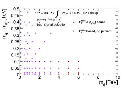
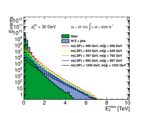
Refer to caption
Figure 41: The choice of analysis that lead to the best discovery reach for a given point in parameter space for an integrated luminosity of 3000 fb-1 at a 100100100 TeV proton collider for the compressed region of the squark-neutralino Simplified Model with light flavor decays. The colors refer to the analyses as presented above: red circle = leading jet based, purple circle = ETmisssuperscriptsubscript𝐸𝑇missE_{T}^{\mathrm{miss}}-based.
Refer to caption
Figure 42: Histogram of ETmisssuperscriptsubscript𝐸𝑇missE_{T}^{\mathrm{miss}} for signal and background at a 100100100 TeV proton collider after the preselection for a range of squark and neutralino masses in the compressed region.
(mq~,mχ~10)subscript𝑚~𝑞subscript𝑚subscriptsuperscript~𝜒01\big{(}m_{\widetilde{q}},\,m_{\widetilde{\chi}^{0}_{1}}\big{)}\quad [GeV]
Cut V𝑉V+jets tt¯𝑡¯𝑡t\,\overline{t} Total BG (1995, 1990)19951990(1995,\,1990) (2512, 2507)25122507(2512,\,2507) (5012, 5007)50125007(5012,\,5007)
Preselection 1.7×10101.7superscript10101.7\times 10^{10} 7.0×1097.0superscript1097.0\times 10^{9} 2.4×10102.4superscript10102.4\times 10^{10} 2.0×1062.0superscript1062.0\times 10^{6} 6.4×1056.4superscript1056.4\times 10^{5} 1.4×1041.4superscript1041.4\times 10^{4}
pTleadjet>110 GeV,|ηleadjet|<2.4formulae-sequencesuperscriptsubscript𝑝𝑇leadjet110 GeVsuperscript𝜂leadjet2.4p_{T}^{\text{leadjet}}>110\text{ GeV},|\eta^{\text{leadjet}}|<2.4 1.2×10101.2superscript10101.2\times 10^{10} 6.1×1096.1superscript1096.1\times 10^{9} 1.9×10101.9superscript10101.9\times 10^{10} 2.0×1062.0superscript1062.0\times 10^{6} 6.4×1056.4superscript1056.4\times 10^{5} 1.4×1041.4superscript1041.4\times 10^{4}
ETmiss>3 TeVsuperscriptsubscript𝐸𝑇miss3 TeVE_{T}^{\mathrm{miss}}>3\text{ TeV} 1.3×1051.3superscript1051.3\times 10^{5} 2.0×1042.0superscript1042.0\times 10^{4} 1.5×1051.5superscript1051.5\times 10^{5} 4.1×1044.1superscript1044.1\times 10^{4} 1.9×1041.9superscript1041.9\times 10^{4} 935935935
ETmiss>6 TeVsuperscriptsubscript𝐸𝑇miss6 TeVE_{T}^{\mathrm{miss}}>6\text{ TeV} 3.6×1033.6superscript1033.6\times 10^{3} 229 3.8×1033.8superscript1033.8\times 10^{3} 2.3×1032.3superscript1032.3\times 10^{3} 1.×1031.\times 10^{3} 116116116
ETmiss>9 TeVsuperscriptsubscript𝐸𝑇miss9 TeVE_{T}^{\mathrm{miss}}>9\text{ TeV} 100100100 999 109109109 206206206 130130130 171717
Table 13: Event yields for background and selected signal points for s=100𝑠100\sqrt{s}=100 TeV and 300030003000 fb-1 in the event selection with cuts on ETmisssuperscriptsubscript𝐸𝑇missE_{T}^{\mathrm{miss}}.

6.6   Results: 100 TeV

The results for the squark neutralino model in the compressed region of parameter space are given in Fig. 43. As discussed above, only the ETmisssuperscriptsubscript𝐸𝑇missE_{T}^{\mathrm{miss}} based strategy (see Sec. 4) is relevant for this model at a 100100100 TeV proton collider. It is possible to exclude (discover) squarks in the degenerate limit with mass less than 4 TeV(3 TeV)similar-toabsent4 TeV3 TeV\sim 4{\text{ TeV}}(3{\text{ TeV}}) with 3000 fb13000superscript fb13000\text{ fb}^{-1} of data. This improves the exclusion (discovery) reach near the degenerate limit compared to the HTsubscript𝐻𝑇H_{T}-based analysis described in Sec. 5 by roughly 1.5 TeV(1.8 TeV)1.5 TeV1.8 TeV1.5{\text{ TeV}}(1.8{\text{ TeV}}) for Δ200 GeVless-than-or-similar-toΔ200 GeV\Delta\lesssim 200{\text{ GeV}}. Note that given our results for the compressed gluino-neutralino study in Sec. 4.10 above, pileup is not expected to have a significant impact on these conclusions. This search demonstrates that a 100100100 TeV machine will be relevant to our understanding of the difficult to probe compressed region of this model.
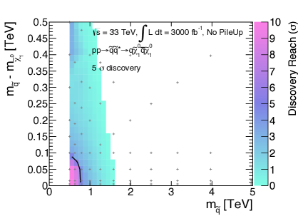
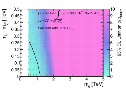
Refer to caption
Refer to caption
Figure 43: Results for the compressed squark-neutralino model with light flavor decays at a 100100100 TeV proton collider are given in the mq~mχ~10subscript𝑚~𝑞subscript𝑚superscriptsubscript~𝜒10m_{\widetilde{q}}-m_{\widetilde{\chi}_{1}^{0}} versus mg~subscript𝑚~𝑔m_{\widetilde{g}} plane. The left [right] plot shows the expected 5σ5𝜎5\sigma discovery reach [95% confidence level upper limits] for squark-anti-squark pair production. Mass points to the left/below the contours are expected to be probed at 300030003000 fb-1 [right]. A 20% systematic uncertainty is assumed for the background and pileup is not included.

6.7   Comparing Colliders

The compressed region of the squark-neutralino model has a similar signature to the compressed gluino-neutralino model with light flavor decays. However, the squark-neutralino model is more difficult to probe due to the substantially smaller production cross section. Since this model provides a more challenging scenario, it is interesting to understand the impact that can be made on exploring the parameter space with different collider scenarios. Figure 44 shows the 5σ5𝜎5\sigma discovery reach [95%percent9595\% CL exclusion] for two choices of integrated luminosity at 141414 TeV, along with the reach using the full data set assumed for 333333 and 100100100 TeV.

In general, we find that due to the small cross sections, it is very difficult to distinguish this model from background with discovery level significance. Consequentially, the discovery reach does not appear to significantly improve with the 141414 TeV luminosity upgrade. The discovery reach increases by a factor of 6similar-toabsent6\sim 6 from 141414 TeV to 100100100 TeV, but in absolute terms remains small. The exclusion reach for the compressed squark-neutralino model is more favorable in comparison. At this level of significance the background systematics are less difficult to overcome, and the limits scale much more favorably with luminosity and CM energy. For higher center-of-mass-energy, these searches specially targeted at the compressed region also become more and more important to fill in the gap in the reach of the untargeted search described in Sec. 5. Figure 44 makes a compelling case for investing in future proton colliders which can operate at these high energies.
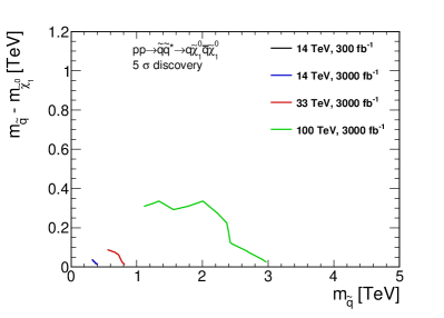
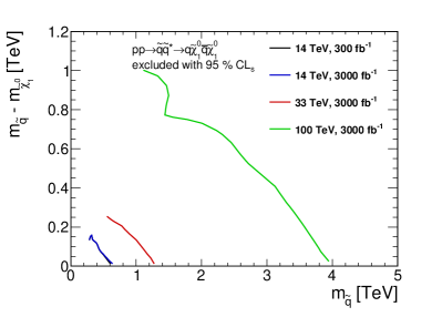
Refer to caption
Refer to caption
Figure 44: Results for the squark-neutralino model with light flavor decays for the analyses that target the compressed region of parameter space. The left [right] panel shows the 5σ5𝜎5\,\sigma discovery reach [95%percent9595\% CL exclusion] for the four collider scenarios studied here. A 20%percent2020\% systematic uncertainty is assumed and pileup is not included.

7 The Gluino-Squark-Neutralino Model

In the “gluino-squark-neutralino model”, the gluino g~~𝑔\widetilde{g} and the first and second generation squarks q~~𝑞\widetilde{q} are all allowed to be kinematically accessible. The only relevant parameters are the squark mass mq~subscript𝑚~𝑞m_{\widetilde{q}}, which is taken to be universal for the first two generations, the gluino mass mg~subscript𝑚~𝑔m_{\widetilde{g}}, and the neutralino mass mχ~0subscript𝑚superscript~𝜒0m_{\widetilde{\chi}^{0}}. For this study we fix the neutralino mass mχ~0=1GeVsubscript𝑚superscript~𝜒01GeVm_{\widetilde{\chi}^{0}}=1{\rm~{}GeV}, which captures the relevant kinematics for mg~,mq~mχ~0much-greater-thansubscript𝑚~𝑔subscript𝑚~𝑞subscript𝑚superscript~𝜒0m_{\widetilde{g}},m_{\widetilde{q}}\gg m_{\widetilde{\chi}^{0}}. The decay mode is chosen depending on the mass hierarchy. The model is summarized as:

BSM particles production decay
g~,q~,χ~10~𝑔~𝑞subscriptsuperscript~𝜒01\widetilde{g},\,\widetilde{q},\,\widetilde{\chi}^{0}_{1} ppg~g~𝑝𝑝~𝑔~𝑔p\,p\rightarrow\widetilde{g}\,\,\widetilde{g} g~{q~q¯formg~>mq~qq¯χ~10formg~mq~qq¯χ~10formg~<mq~~𝑔cases~𝑞¯𝑞forsubscript𝑚~𝑔subscript𝑚~𝑞𝑞¯𝑞subscriptsuperscript~𝜒01similar-to-or-equalsforsubscript𝑚~𝑔subscript𝑚~𝑞𝑞¯𝑞subscriptsuperscript~𝜒01forsubscript𝑚~𝑔subscript𝑚~𝑞\widetilde{g}\rightarrow\begin{cases}\widetilde{q}\,\,\overline{q}&\text{for}\,\,\,m_{\widetilde{g}}>m_{\widetilde{q}}\\ q\,\overline{q}\,\widetilde{\chi}^{0}_{1}&\text{for}\,\,\,m_{\widetilde{g}}\simeq m_{\widetilde{q}}\\ q\,\overline{q}\,\widetilde{\chi}^{0}_{1}&\text{for}\,\,\,m_{\widetilde{g}}<m_{\widetilde{q}}\end{cases}
ppg~q~𝑝𝑝~𝑔~𝑞p\,p\rightarrow\widetilde{g}\,\,\widetilde{q}
ppg~q~𝑝𝑝~𝑔superscript~𝑞p\,p\rightarrow\widetilde{g}\,\,\widetilde{q}^{*}
ppq~q~𝑝𝑝~𝑞superscript~𝑞p\,p\rightarrow\widetilde{q}\,\,\widetilde{q}^{*} q~{qχ~10formg~>mq~qχ~10formg~mq~qg~formg~<mq~~𝑞cases𝑞subscriptsuperscript~𝜒01forsubscript𝑚~𝑔subscript𝑚~𝑞𝑞subscriptsuperscript~𝜒01similar-to-or-equalsforsubscript𝑚~𝑔subscript𝑚~𝑞𝑞~𝑔forsubscript𝑚~𝑔subscript𝑚~𝑞\widetilde{q}\rightarrow\begin{cases}q\,\widetilde{\chi}^{0}_{1}&\text{for}\,\,\,m_{\widetilde{g}}>m_{\widetilde{q}}\\ q\,\widetilde{\chi}^{0}_{1}&\text{for}\,\,\,m_{\widetilde{g}}\simeq m_{\widetilde{q}}\\ q\,\widetilde{g}&\text{for}\,\,\,m_{\widetilde{g}}<m_{\widetilde{q}}\end{cases}
ppq~q~𝑝𝑝~𝑞~𝑞p\,p\rightarrow\widetilde{q}\,\,\widetilde{q}

For a full MSSM model, which in particular would imply a specific neutralino composition, there will in general be a non-zero branching ratio for the squark to decay to a neutralino and a quark when kinematically allowed. If the decay directly to a gluino is kinematically allowed however it will tend to dominate, and in this study for simplicity we assume that the squark is weakly coupled to the neutralino and decays to the gluino proceed with 100% branching ratio when kinematically allowed. Likewise for mg~>mq~subscript𝑚~𝑔subscript𝑚~𝑞m_{\widetilde{g}}>m_{\widetilde{q}}, the branching ratio of the gluino to 3-body versus 2-body decays depends on the masses and coupling of the squarks to the neutralino, and we take the 2-body branching ratio to be 100% in this region of parameter space. To capture the transition region where mg~mq~similar-to-or-equalssubscript𝑚~𝑔subscript𝑚~𝑞m_{\widetilde{g}}\simeq m_{\widetilde{q}}, parameter choices along the line mg~=mq~subscript𝑚~𝑔subscript𝑚~𝑞m_{\widetilde{g}}=m_{\widetilde{q}} are included; the gluino decay is taken to be 3-body and the squarks are assumed to decay directly to the neutralino.

This model is a good proxy for comparing the power of searches which rely on the traditional jets and ETmisssuperscriptsubscript𝐸𝑇missE_{T}^{\mathrm{miss}} style hadron collider search strategy to discriminate against background. The final state ranges from two to four (or more) hard jets from the decay (depending on the production channel) and missing energy. The current preliminary limits on this model using 202020 fb-1 of 888 TeV data are mg~=1750 GeVsubscript𝑚~𝑔1750 GeVm_{\widetilde{g}}=1750\text{ GeV} and mq~=1600 GeVsubscript𝑚~𝑞1600 GeVm_{\widetilde{q}}=1600\text{ GeV} (ATLAS [29]) assuming a massless neutralino.

We simulated matched MadGraph samples for (g~g~),(q~q~),(q~q~),(g~q~),(g~q~)~𝑔~𝑔~𝑞superscript~𝑞~𝑞~𝑞~𝑔~𝑞~𝑔superscript~𝑞\big{(}\widetilde{g}\,\widetilde{g}\big{)},\,\big{(}\widetilde{q}\,\widetilde{q}^{*}\big{)},\,\big{(}\widetilde{q}\,\widetilde{q}\big{)},\,\big{(}\widetilde{g}\,\widetilde{q}\big{)},\,\big{(}\widetilde{g}\,\widetilde{q}^{*}\big{)} production with up to 2 additional generator level jets for the following points in parameter space:

BSM particles masses
mg~subscript𝑚~𝑔m_{\widetilde{g}} [14 TeV]delimited-[]14 TeV\big{[}14{\text{ TeV}}\big{]} (315,397,500,629,792,997,1255,1580,1989,2489,2989,(315,397,500,629,792,997,1255,1580,1989,2489,2989,
 3489,3989,4489) GeV\,3489,3989,4489){\text{ GeV}}
mg~subscript𝑚~𝑔m_{\widetilde{g}} [33 TeV]delimited-[]33 TeV\big{[}33{\text{ TeV}}\big{]} (1000,1259,1585,1995,2512,3162,3981,4981,5981,6981,(1000,1259,1585,1995,2512,3162,3981,4981,5981,6981,
7981,8981,9981) GeV7981,8981,9981\,){\text{ GeV}}
mg~subscript𝑚~𝑔m_{\widetilde{g}} [100 TeV]delimited-[]100 TeV\big{[}100{\text{ TeV}}\big{]} (1000,1259,1585,1995,2512,3162,3981,5012,6310,7944,(1000,1259,1585,1995,2512,3162,3981,5012,6310,7944,
9944,11944,13944,15944,17944,19944,21944,23944) GeV9944,11944,13944,15944,17944,19944,21944,23944\,){\text{ GeV}}
mq~subscript𝑚~𝑞m_{\widetilde{q}} [14 TeV]delimited-[]14 TeV\big{[}14{\text{ TeV}}\big{]} (315,397,500,629,792,997,1255,1580,1989,2489,2989,(315,397,500,629,792,997,1255,1580,1989,2489,2989,
 3489,3989,4489) GeV\,3489,3989,4489){\text{ GeV}}
mq~subscript𝑚~𝑞m_{\widetilde{q}} [33 TeV]delimited-[]33 TeV\big{[}33{\text{ TeV}}\big{]} (1000,1259,1585,1995,2512,3162,3981,4981,5981,6981,(1000,1259,1585,1995,2512,3162,3981,4981,5981,6981,
7981,8981,9981) GeV7981,8981,9981\,){\text{ GeV}}
mq~subscript𝑚~𝑞m_{\widetilde{q}} [100 TeV]delimited-[]100 TeV\big{[}100{\text{ TeV}}\big{]} (1000,1259,1585,1995,2512,3162,3981,5012,6310,7944,(1000,1259,1585,1995,2512,3162,3981,5012,6310,7944,
9944,11944,13944,15944,17944,19944,21944,23944) GeV9944,11944,13944,15944,17944,19944,21944,23944\,){\text{ GeV}}
mχ~10subscript𝑚subscriptsuperscript~𝜒01m_{\widetilde{\chi}^{0}_{1}} 1 GeV1 GeV1{\text{ GeV}}

The signatures of this model are essentially a mixture of the gluino-neutralino and squark-neutralino Simplified Models except for slight variations in the kinematics due to the presence of on-shell states in the decays. Therefore, the dominant backgrounds will be the same as described in Sec. 3.1, and we use the same search strategy described in detail in Sec. 3.2. Again, based on the results of studying the effect of pile-up on this search strategy in Sec. 3.12, we present results only for the no pile-up scenario and expect that that pileup will not have a significant impact on the results.

When both the gluino and squarks are kinematically accessible, the total cross section for this Simplified Model is significantly enhanced with respect to the limit where either particle is decoupled due to the presence of the associated production channel g~q~~𝑔~𝑞\widetilde{g}\,\widetilde{q} and also due to t𝑡t-channel diagrams which open the important q~q~~𝑞~𝑞\widetilde{q}\,\widetilde{q} channel and tend to dominate the q~q~~𝑞superscript~𝑞\widetilde{q}\,\widetilde{q}^{*} cross sections. It is important to note that even when the squarks or gluinos are kinematically inaccessible these t-channel processes still can dominate the cross section. For this reason the limits we obtain within the scanned range of gluino and squark masses do not reach the asymptotic values that can be inferred from the gluino-neutralino and squark-neutralino Simplified Models.

7.1   Analysis: 14 TeV

Figure 45 gives histograms for ETmisssuperscriptsubscript𝐸𝑇missE_{T}^{\mathrm{miss}} [left] and HTsubscript𝐻𝑇H_{T} [right] for two example models at the 141414 TeV LHC. Comparing with the analogous gluino-neutralino (Fig. 2) and squark-neutralino (Fig. 28) distributions, it is clear that the total BSM cross section in this model is enhanced. This will lead to a significant improvement in mass reach with respect to the previous results.

The number of events that result from the cut flow used in this search are shown in Table 14. By comparing the optimal cuts which result from this analysis to the to the cuts employed for the gluino-neutralino model in Table 1 and the squark-neutralino model in Table 8, it is clear that the optimization procedure can take advantage of the the larger cross sections by utilizing significantly harder cuts.
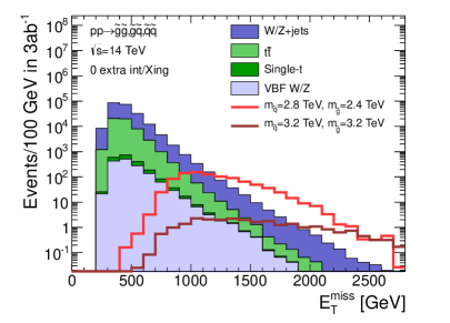
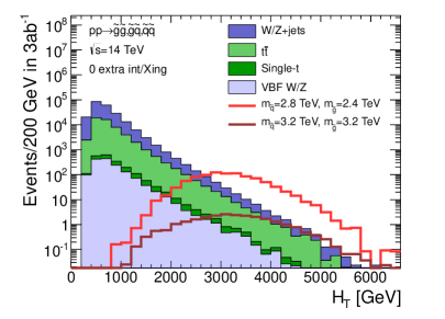
Refer to caption
Refer to caption
Figure 45: Histogram of ETmisssuperscriptsubscript𝐸𝑇missE_{T}^{\mathrm{miss}} [left] and HTsubscript𝐻𝑇H_{T} [right] after preselection cuts for background and a range of gluino-squark models at a 141414 TeV proton collider. The neutralino mass is 1 GeV1 GeV1{\text{ GeV}} for all signal models.
(mg~,mq~)subscript𝑚~𝑔subscript𝑚~𝑞\left(m_{\widetilde{g}},m_{\widetilde{q}}\right)\,\,\,\,\,\,\,\,\, [TeV]
Cut V𝑉V+jets tt¯𝑡¯𝑡t\bar{t} Total BG (2.4,2.8)2.42.8(2.4,2.8) (3.2,3.2)3.23.2(3.2,3.2)
Preselection 2.07×1072.07superscript1072.07\times 10^{7} 2.47×1072.47superscript1072.47\times 10^{7} 4.54×1074.54superscript1074.54\times 10^{7} 2.75×1032.75superscript1032.75\times 10^{3} 136
ETmiss/HT>15 GeV1/2superscriptsubscript𝐸𝑇misssubscript𝐻𝑇15superscript GeV12E_{T}^{\mathrm{miss}}/\sqrt{H_{T}}>15\text{ GeV}^{1/2} 4.45×1054.45superscript1054.45\times 10^{5} 1.20×1051.20superscript1051.20\times 10^{5} 5.65×1055.65superscript1055.65\times 10^{5} 1.34×1031.34superscript1031.34\times 10^{3} 109
pTleading<0.4×HTsuperscriptsubscript𝑝𝑇leading0.4subscript𝐻𝑇p_{T}^{\text{leading}}<0.4\times H_{T} 1.69×1051.69superscript1051.69\times 10^{5} 5.16×1045.16superscript1045.16\times 10^{4} 2.21×1052.21superscript1052.21\times 10^{5} 937 25.4
ETmiss>1250superscriptsubscript𝐸𝑇miss1250E_{T}^{\mathrm{miss}}>1250 GeV 10.8 5 15.8 264 12.8
HT>3000subscript𝐻𝑇3000H_{T}>3000 GeV
ETmiss>1850superscriptsubscript𝐸𝑇miss1850E_{T}^{\mathrm{miss}}>1850 GeV 1 0.2 1.2 30.5 6.1
HT>2850subscript𝐻𝑇2850H_{T}>2850 GeV
Table 14: Number of expected events for s=14𝑠14\sqrt{s}=14 TeV with 3000 fb-1 integrated luminosity for the background processes and selected gluino and squark masses for the gluino-squark model with light flavor decays. The neutralino mass is 1 GeV1 GeV1{\text{ GeV}}. Two choices of cuts on ETmisssuperscriptsubscript𝐸𝑇missE_{T}^{\mathrm{miss}} and HTsubscript𝐻𝑇H_{T} are provided, and for each mass column the entry in the row corresponding to the “optimal” cuts is marked in red.

7.2   Results: 14 TeV

The results for the gluino-squark-neutralino model are shown in Fig. 46. In the bulk of the parameter space, the 14 TeV14 TeV14{\text{ TeV}} LHC with 3000 fb13000superscript fb13000\text{ fb}^{-1} could discover a model with mg~3 TeVsimilar-to-or-equalssubscript𝑚~𝑔3 TeVm_{\widetilde{g}}\simeq 3{\text{ TeV}} and mq~3 TeVsimilar-to-or-equalssubscript𝑚~𝑞3 TeVm_{\widetilde{q}}\simeq 3{\text{ TeV}}. When compared to the maximal reach for the gluino-neutralino model of mg~2.3 TeVsimilar-to-or-equalssubscript𝑚~𝑔2.3 TeVm_{\widetilde{g}}\simeq 2.3{\text{ TeV}} as shown in Fig. 3, the large cross section for the additional channels explains this 30%similar-toabsentpercent30\sim 30\% improvement.

Using the NLO gluino pair production cross section one can make a very naive estimate for the reach of a given collider. We found the choice of gluino and squark masses which would yield a fixed number of events at 14 TeV14 TeV14{\text{ TeV}} and 300 fb1300superscript fb1300\text{ fb}^{-1} (3000 fb1)3000superscript fb1\big{(}3000\text{ fb}^{-1}\big{)} for three choices in the mq~mg~subscript𝑚~𝑞subscript𝑚~𝑔m_{\widetilde{q}}-m_{\widetilde{g}} plane: there would be 101010 events when mg~=mq~=3.5 TeV(3.9 TeV)subscript𝑚~𝑔subscript𝑚~𝑞3.5 TeV3.9 TeVm_{\widetilde{g}}=m_{\widetilde{q}}=3.5{\text{ TeV}}\,(3.9{\text{ TeV}}); when mg~=2.7 TeV(3.2 TeV)subscript𝑚~𝑔2.7 TeV3.2 TeVm_{\widetilde{g}}=2.7{\text{ TeV}}\,(3.2{\text{ TeV}}) and the squark mass is at the edge of the region simulated; and when mq~=3.3 TeV(3.9 TeV)subscript𝑚~𝑞3.3 TeV3.9 TeVm_{\widetilde{q}}=3.3{\text{ TeV}}\,(3.9{\text{ TeV}}) and the gluino mass is at the edge of the region simulated. This roughly corresponds to the maximal possible reach one could expect for a given luminosity using 14 TeV14 TeV14{\text{ TeV}} proton collisions.

Using a realistic simulation framework along with the search strategy employed here the 14 TeV14 TeV14{\text{ TeV}} 300 fb1300superscript fb1300\text{ fb}^{-1} limits are projected to be mg~=mq~=2.8subscript𝑚~𝑔subscript𝑚~𝑞2.8m_{\widetilde{g}}=m_{\widetilde{q}}=2.8 (corresponding to 155 events); mg~=2.4 TeVsubscript𝑚~𝑔2.4 TeVm_{\widetilde{g}}=2.4{\text{ TeV}} (corresponding to 43 events) and the squark mass is at the edge of the region simulated; mq~=2.1 TeVsubscript𝑚~𝑞2.1 TeVm_{\widetilde{q}}=2.1{\text{ TeV}} (corresponding to 774 events) and the gluino mass is at the edge of the region simulated. The 14 TeV14 TeV14{\text{ TeV}} 3000 fb13000superscript fb13000\text{ fb}^{-1} limits are projected to be mg~=mq~=3.2subscript𝑚~𝑔subscript𝑚~𝑞3.2m_{\widetilde{g}}=m_{\widetilde{q}}=3.2 (corresponding to 293 events); mg~=3.0 TeVsubscript𝑚~𝑔3.0 TeVm_{\widetilde{g}}=3.0{\text{ TeV}} (corresponding to 23 events) and the squark mass is at the edge of the region simulated; mq~=2.7 TeVsubscript𝑚~𝑞2.7 TeVm_{\widetilde{q}}=2.7{\text{ TeV}} (corresponding to 953 events) and the gluino mass is at the edge of the region simulated. Clearly the search does better with light gluinos. This is likely related to the four jet preselection requirement. It would be investigating to understand what additional search regions could be used to push the mass reach even further; this is beyond the scope of this work.
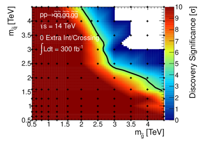
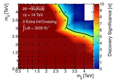
Refer to caption
Refer to caption
Refer to caption
Refer to caption
Figure 46: Results for the gluino-squark model with a massless neutralino are given in the mg~subscript𝑚~𝑔m_{\widetilde{g}} versus mq~subscript𝑚~𝑞m_{\widetilde{q}} plane. The top [bottom] row shows the expected 5σ5𝜎5\sigma discovery reach [95% confidence level upper limits] for the combined production channels at the 141414 TeV LHC. Mass points to the left/below the contours are expected to be probed at 300 fb-1 [left] and 3000 fb-1 [right]. A 20% systematic uncertainty is assumed and pileup is not included.

7.3   Analysis: 33 TeV

Figure 47 gives histograms for ETmisssuperscriptsubscript𝐸𝑇missE_{T}^{\mathrm{miss}} [left] and HTsubscript𝐻𝑇H_{T} [right] for two example models at the 333333 TeV LHC. Comparing with the analogous gluino-neutralino (Fig. 4) and squark-neutralino (Fig. 30) distributions, it is clear that the total BSM cross section in this model is enhanced. This will lead to a significant improvement in mass reach with respect to the previous results.

The number of events that result from the cut flow used in this search are shown in Table 15. By comparing the optimal cuts which result from this analysis to the cuts employed for the gluino-neutralino model in Table 2 and the squark-neutralino model in Table 9, it is clear that the optimization procedure can take advantage of the the larger cross sections by utilizing significantly harder cuts.
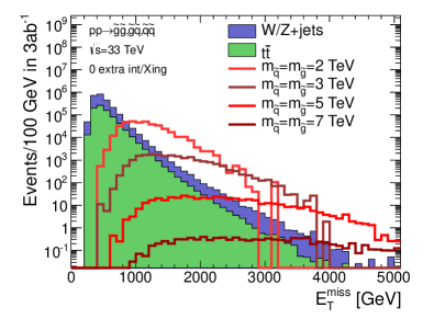
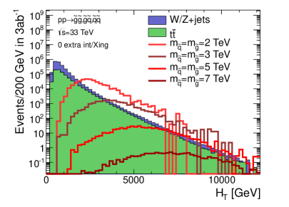
Refer to caption
Refer to caption
Figure 47: Histogram of ETmisssuperscriptsubscript𝐸𝑇missE_{T}^{\mathrm{miss}} [left] and HTsubscript𝐻𝑇H_{T} [right] after preselection cuts for background and a range of gluino-squark models at a 333333 TeV proton collider. The neutralino mass is 1 GeV1 GeV1{\text{ GeV}} for all signal models.
(mg~,mq~)subscript𝑚~𝑔subscript𝑚~𝑞\left(m_{\widetilde{g}},m_{\widetilde{q}}\right)\,\,\,\,\,\,\,\,\, [TeV]
Cut V𝑉V+jets tt¯𝑡¯𝑡t\overline{t} Total BG (3.2,3.2)3.23.2(3.2,3.2) (6.0,6.0)6.06.0(6.0,6.0)
PreselectionPreselection\mathrm{Preselection} 1.55×1081.55superscript1081.55\times 10^{8} 2.86×1082.86superscript1082.86\times 10^{8} 4.42×1084.42superscript1084.42\times 10^{8} 8.64×1048.64superscript1048.64\times 10^{4} 361361361
ETmiss/HT>15 GeV1/2superscriptsubscript𝐸𝑇misssubscript𝐻𝑇15superscript GeV12E_{T}^{\mathrm{miss}}/\sqrt{H_{T}}>15{\text{ GeV}}^{1/2} 4.50×1064.50superscript1064.50\times 10^{6} 1.93×1061.93superscript1061.93\times 10^{6} 6.44×1066.44superscript1066.44\times 10^{6} 6.55×1046.55superscript1046.55\times 10^{4} 321321321
pTleading<0.4HTsuperscriptsubscript𝑝Tleading0.4subscript𝐻𝑇p_{\mathrm{T}}^{\mathrm{leading}}<0.4H_{T} 1.70×1061.70superscript1061.70\times 10^{6} 8.02×1058.02superscript1058.02\times 10^{5} 2.50×1062.50superscript1062.50\times 10^{6} 2.14×1042.14superscript1042.14\times 10^{4} 69.869.869.8
ETmiss>2650 GeVsuperscriptsubscript𝐸𝑇miss2650 GeVE_{T}^{\mathrm{miss}}>2650{\text{ GeV}} 60.460.460.4 16.416.416.4 76.876.876.8 1.79×1031.79superscript1031.79\times 10^{3} 40.1
HT>2700 GeVsubscript𝐻𝑇2700 GeVH_{T}>2700{\text{ GeV}}
ETmiss>3700 GeVsuperscriptsubscript𝐸𝑇miss3700 GeVE_{T}^{\mathrm{miss}}>3700{\text{ GeV}} 1.11.11.1 0.30.30.3 1.31.31.3 30.430.430.4 14.214.214.2
HT>5350 GeVsubscript𝐻𝑇5350 GeVH_{T}>5350{\text{ GeV}}
Table 15: Number of expected events for s=33𝑠33\sqrt{s}=33 TeV with 3000 fb-1 integrated luminosity for the background processes and selected gluino and squark masses for the gluino-squark model with light flavor decays. The neutralino mass is 1 GeV1 GeV1{\text{ GeV}}. Three choices of cuts on ETmisssuperscriptsubscript𝐸𝑇missE_{T}^{\mathrm{miss}} and HTsubscript𝐻𝑇H_{T} are provided, and for each mass column the entry in the row corresponding to the “optimal” cuts is marked in red.

7.4   Results: 33 TeV

The results for the gluino-squark-neutralino model are shown in Fig. 48. In the bulk of the parameter space, a 33 TeV33 TeV33{\text{ TeV}} proton collider with 3000 fb13000superscript fb13000\text{ fb}^{-1} could discover a model with mg~6.5 TeVsimilar-to-or-equalssubscript𝑚~𝑔6.5 TeVm_{\widetilde{g}}\simeq 6.5{\text{ TeV}} and mq~6 TeVsimilar-to-or-equalssubscript𝑚~𝑞6 TeVm_{\widetilde{q}}\simeq 6{\text{ TeV}}. When compared to the maximal reach for the gluino-neutralino model of mg~4.8 TeVsimilar-to-or-equalssubscript𝑚~𝑔4.8 TeVm_{\widetilde{g}}\simeq 4.8{\text{ TeV}} as shown in Fig. 5, the large cross section for the additional channels explains this 30%similar-toabsentpercent30\sim 30\% improvement.

Using the NLO gluino pair production cross section one can make a very naive estimate for the reach of a given collider. We found the choice of gluino and squark masses which would yield a fixed number of events at 33 TeV33 TeV33{\text{ TeV}} and 3000 fb13000superscript fb13000\text{ fb}^{-1} for three choices in the mq~mg~subscript𝑚~𝑞subscript𝑚~𝑔m_{\widetilde{q}}-m_{\widetilde{g}} plane: there would be 101010 events when mg~=mq~=8.2 TeVsubscript𝑚~𝑔subscript𝑚~𝑞8.2 TeVm_{\widetilde{g}}=m_{\widetilde{q}}=8.2{\text{ TeV}}; when mg~=6.1 TeVsubscript𝑚~𝑔6.1 TeVm_{\widetilde{g}}=6.1{\text{ TeV}} and the squark mass is at the edge of the region simulated; and when mq~=5.5 TeVsubscript𝑚~𝑞5.5 TeVm_{\widetilde{q}}=5.5{\text{ TeV}} and the gluino mass is at the edge of the region simulated. This roughly corresponds to the maximal possible reach one could expect for a given luminosity using 33 TeV33 TeV33{\text{ TeV}} proton collisions.

Using a realistic simulation framework along with the search strategy employed here the 33 TeV33 TeV33{\text{ TeV}} 3000 fb13000superscript fb13000\text{ fb}^{-1} limits are projected to be mg~=mq~=6.8subscript𝑚~𝑔subscript𝑚~𝑞6.8m_{\widetilde{g}}=m_{\widetilde{q}}=6.8 (corresponding to 132 events); mg~=6.1 TeVsubscript𝑚~𝑔6.1 TeVm_{\widetilde{g}}=6.1{\text{ TeV}} (corresponding to 21 events) and the squark mass is at the edge of the region simulated; mq~=5.5 TeVsubscript𝑚~𝑞5.5 TeVm_{\widetilde{q}}=5.5{\text{ TeV}} (corresponding to 473 events) and the gluino mass is at the edge of the region simulated. Clearly the search does better with light gluinos. Furthermore, we find that we are closer to the ideal limit than in the 14 TeV14 TeV14{\text{ TeV}} case. Both of these facts are likely related to the four jet preselection requirement. While investigating the reach that could be extracted using additional search regions is beyond the scope of this work, it would be interesting to understand what it takes to push the mass reach even further.
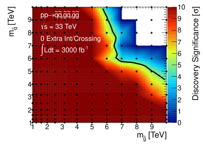
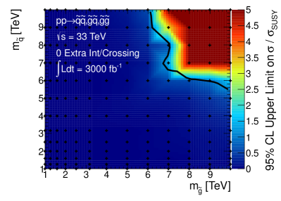
Refer to caption
Refer to caption
Figure 48: Results for the gluino-squark model with a massless neutralino are given in the mg~subscript𝑚~𝑔m_{\widetilde{g}} versus mq~subscript𝑚~𝑞m_{\widetilde{q}} plane. The left [right] panel shows the expected 5σ5𝜎5\sigma discovery reach [95% confidence level upper limits] for the combined production channels at a 100100100 TeV proton collider. Mass points to the left/below the contours are expected to be probed with 3000 fb-1 of data. A 20% systematic uncertainty is assumed and pileup is not included.

7.5   Analysis: 100 TeV

Figure 49 gives histograms for ETmisssuperscriptsubscript𝐸𝑇missE_{T}^{\mathrm{miss}} [left] and HTsubscript𝐻𝑇H_{T} [right] for two example models at a 100100100 TeV proton collider. Comparing with the analogous gluino-neutralino (Fig. 6) and squark-neutralino (Fig. 32) distributions, it is clear that the total BSM cross section in this model is enhanced. This will lead to a significant improvement in mass reach with respect to the previous results.

The number of events that result from the cut flow used in this search are shown in Table 16. Comparing the optimal cuts which result for this model to the cuts employed for the gluino-neutralino model in Table 3 and the squark-neutralino model in Table 10, it is clear that the optimization procedure can take advantage of the the larger cross sections by utilizing significantly harder cuts.
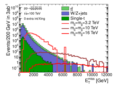
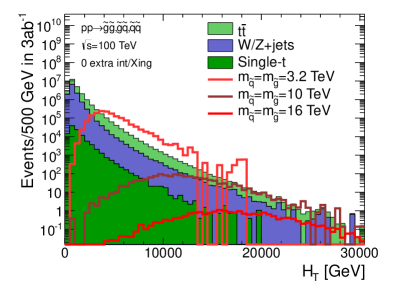
Refer to caption
Refer to caption
Figure 49: Histogram of ETmisssuperscriptsubscript𝐸𝑇missE_{T}^{\mathrm{miss}} [left] and HTsubscript𝐻𝑇H_{T} [right] after preselection cuts for background and a range of gluino-squark models at a 100100100 TeV proton collider. The neutralino mass is 1 GeV1 GeV1{\text{ GeV}} for all signal models.
(mg~,mq~)subscript𝑚~𝑔subscript𝑚~𝑞\left(m_{\widetilde{g}},m_{\widetilde{q}}\right)\,\,\,\,\,\,\,\,\, [TeV]
Cut V𝑉V+jets tt¯𝑡¯𝑡t\overline{t} Total BG (8,8)88(8,8) (16,16)1616(16,16)
PreselectionPreselection\mathrm{Preselection} 1.64×1091.64superscript1091.64\times 10^{9} 3.33×1093.33superscript1093.33\times 10^{9} 4.97×1094.97superscript1094.97\times 10^{9} 2.69×1042.69superscript1042.69\times 10^{4} 111
ETmiss/HT>15 GeV1/2superscriptsubscript𝐸𝑇misssubscript𝐻𝑇15superscript GeV12E_{T}^{\mathrm{miss}}/\sqrt{H_{T}}>15{\text{ GeV}}^{1/2} 3.59×1073.59superscript1073.59\times 10^{7} 3.31×1073.31superscript1073.31\times 10^{7} 6.90×1076.90superscript1076.90\times 10^{7} 2.41×1042.41superscript1042.41\times 10^{4} 107107107
pTleading<0.4×HTsuperscriptsubscript𝑝𝑇leading0.4subscript𝐻𝑇p_{T}^{\mathrm{leading}}<0.4\times H_{T} 1.19×1071.19superscript1071.19\times 10^{7} 1.25×1071.25superscript1071.25\times 10^{7} 2.44×1072.44superscript1072.44\times 10^{7} 7.34×1037.34superscript1037.34\times 10^{3} 20.520.520.5
ETmiss>5700 GeVsuperscriptsubscript𝐸𝑇miss5700 GeVE_{T}^{\mathrm{miss}}>5700{\text{ GeV}} 131313 14.914.914.9 27.827.827.8 771771771 121212
HT>8000 GeVsubscript𝐻𝑇8000 GeVH_{T}>8000{\text{ GeV}}
ETmiss>5800 GeVsuperscriptsubscript𝐸𝑇miss5800 GeVE_{T}^{\mathrm{miss}}>5800{\text{ GeV}} 0.40.40.4 2.52.52.5 2.92.92.9 41.741.741.7 5.35.35.3
HT>17800 GeVsubscript𝐻𝑇17800 GeVH_{T}>17800{\text{ GeV}}
Table 16: Number of expected events for s=100𝑠100\sqrt{s}=100 TeV with 3000 fb-1 integrated luminosity for the background processes and selected gluino and squark masses for the gluino-squark model with light flavor decays. The neutralino mass is 1 GeV1 GeV1{\text{ GeV}}. Two choices of cuts on ETmisssuperscriptsubscript𝐸𝑇missE_{T}^{\mathrm{miss}} and HTsubscript𝐻𝑇H_{T} are provided, and for each mass column the entry in the row corresponding to the “optimal” cuts is marked in red.

7.6   Results: 100 TeV

The results for the gluino-squark-neutralino model are shown in Fig. 50. In the bulk of the parameter space, a 100 TeV100 TeV100{\text{ TeV}} proton collider with 3000 fb13000superscript fb13000\text{ fb}^{-1} could discover a model with mg~16 TeVsimilar-to-or-equalssubscript𝑚~𝑔16 TeVm_{\widetilde{g}}\simeq 16{\text{ TeV}} and mq~14 TeVsimilar-to-or-equalssubscript𝑚~𝑞14 TeVm_{\widetilde{q}}\simeq 14{\text{ TeV}}. When compared to the maximal reach for the gluino-neutralino model of mg~11 TeVsimilar-to-or-equalssubscript𝑚~𝑔11 TeVm_{\widetilde{g}}\simeq 11{\text{ TeV}} as shown in Fig. 7, the large cross section for the additional channels explains this 30%similar-toabsentpercent30\sim 30\% improvement.

Using the NLO gluino pair production cross section one can make a very naive estimate for the reach of a given collider. The choice of gluino and squark masses which would yield a fixed number of events at 100 TeV100 TeV100{\text{ TeV}} and 3000 fb13000superscript fb13000\text{ fb}^{-1} for three choices in the mq~mg~subscript𝑚~𝑞subscript𝑚~𝑔m_{\widetilde{q}}-m_{\widetilde{g}} plane: there would be 101010 events when mg~=mq~=20.4 TeVsubscript𝑚~𝑔subscript𝑚~𝑞20.4 TeVm_{\widetilde{g}}=m_{\widetilde{q}}=20.4{\text{ TeV}}; when mg~=16.5 TeVsubscript𝑚~𝑔16.5 TeVm_{\widetilde{g}}=16.5{\text{ TeV}} and the squark mass is at the edge of the region simulated; and when mq~=19.6 TeVsubscript𝑚~𝑞19.6 TeVm_{\widetilde{q}}=19.6{\text{ TeV}} and the gluino mass is at the edge of the region simulated. This roughly corresponds to the maximal possible reach one could expect for a given luminosity using 100 TeV100 TeV100{\text{ TeV}} proton collisions.

Using a realistic simulation framework along with the search strategy employed here the 100 TeV100 TeV100{\text{ TeV}} 3000 fb13000superscript fb13000\text{ fb}^{-1} limits are projected to be mg~=mq~=16subscript𝑚~𝑔subscript𝑚~𝑞16m_{\widetilde{g}}=m_{\widetilde{q}}=16 (corresponding to 136 events); mg~=16 TeVsubscript𝑚~𝑔16 TeVm_{\widetilde{g}}=16{\text{ TeV}} (corresponding to 13 events) and the squark mass is at the edge of the region simulated; mq~=14 TeVsubscript𝑚~𝑞14 TeVm_{\widetilde{q}}=14{\text{ TeV}} (corresponding to 169 events) and the gluino mass is at the edge of the region simulated. Clearly the search does better with light gluinos. Furthermore, we find that we are closer to the ideal limit than in the 14 TeV14 TeV14{\text{ TeV}} and 33 TeV33 TeV33{\text{ TeV}} cases. Both of these facts are likely related to the four jet preselection requirement. While investigating the reach that could be extracted using additional search regions is beyond the scope of this work, it would be interesting to understand what it takes to push the mass reach even further.

The next section provides a comparison of the impact that the four collider scenarios studied here can have on the parameter space of this model.
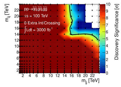
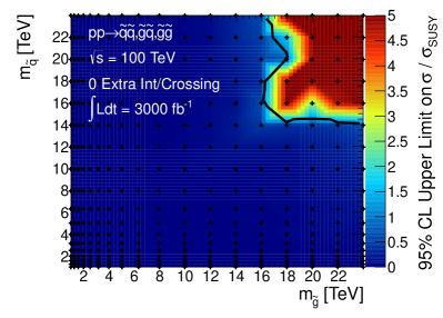
Refer to caption
Refer to caption
Figure 50: Results for the gluino-squark model with a massless neutralino are given in the mg~subscript𝑚~𝑔m_{\widetilde{g}} versus mq~subscript𝑚~𝑞m_{\widetilde{q}} plane. The left [right] panel shows the expected 5σ5𝜎5\sigma discovery reach [95% confidence level upper limits] for the combined production channels at a 100100100 TeV proton collider. Mass points to the left/below the contours are expected to be probed with 3000 fb-1 of data. A 20% systematic uncertainty is assumed and pileup is not included.

7.7   Comparing Colliders

The multi-jet plus ETmisssuperscriptsubscript𝐸𝑇missE_{T}^{\mathrm{miss}} signature of the gluino-squark-neutralino model with light flavor decays provides a useful case study with which to compare the potential impact of different proton colliders. Due to the large production cross sections, this model is also interesting as one of the most striking possible cases of accessible new physics. Figure 51 shows the 5σ5𝜎5\sigma discovery reach [95%percent9595\% CL exclusion] for two choices of integrated luminosity at 141414 TeV, along with the full data set assumed for 333333 and 100100100 TeV. Because the high mass signal regions are relatively low-background for this model, a factor of 101010 increase in luminosity leads to roughly a factor of 10 increase in cross-section reach at edges of the limits. In terms of mass reach, this corresponds roughly to a respectable 500500500 GeV improvement. Again increasing the center-of-mass energy has a tremendous impact on the experimentally available parameter space, since now much heavier gluinos can be produced without relying on the tails of parton distributions to supply the necessary energy. Figure 51 makes a compelling case for investing in future proton colliders which can operate at these high energies.
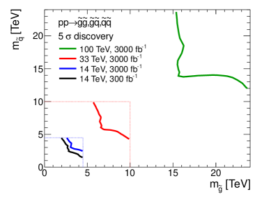
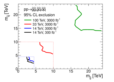
Refer to caption
Refer to caption
Figure 51: Results for the gluino-squark-neutralino model. The neutralino mass is taken to be 1 GeV1 GeV1{\text{ GeV}}. The left [right] panel shows the 5σ5𝜎5\,\sigma discovery reach [95%percent9595\% CL exclusion] for the four collider scenarios studied here. A 20%percent2020\% systematic uncertainty is assumed and pileup is not included.

8 The Gluino-Neutralino Model with Heavy Flavor Decays

In the “gluino-neutralino model with heavy flavor decays”, the gluino g~~𝑔\widetilde{g} is the only kinematically accessible colored particle. The squarks are completely decoupled and do not contribute to gluino production diagrams. The gluino undergoes a prompt three-body decay through off-shell stops, g~tt¯χ~10~𝑔𝑡¯𝑡subscriptsuperscript~𝜒01\widetilde{g}\rightarrow t\,\overline{t}\,\widetilde{\chi}^{0}_{1}, where t𝑡t is the top quark and χ~10subscriptsuperscript~𝜒01\widetilde{\chi}^{0}_{1} is a neutralino LSP. The only two relevant parameters are the gluino mass mg~subscript𝑚~𝑔m_{\widetilde{g}} and the neutralino mass mχ~10subscript𝑚subscriptsuperscript~𝜒01m_{\widetilde{\chi}^{0}_{1}}. This model can be summarized by:

BSM particles production decays
g~,χ~10~𝑔subscriptsuperscript~𝜒01\widetilde{g},\,\widetilde{\chi}^{0}_{1} ppg~g~𝑝𝑝~𝑔~𝑔p\,p\rightarrow\widetilde{g}\,\widetilde{g} g~tt¯χ~10~𝑔𝑡¯𝑡subscriptsuperscript~𝜒01\widetilde{g}\rightarrow t\,\overline{t}\,\widetilde{\chi}^{0}_{1}

This model has a variety of motivations. Perhaps the most compelling are “natural” SUSY scenarios [36, 37, 38, 39, 40], where the stop mass is assumed to be below the (stronger) bounds on first and second generation squark masses; for some examples of explicit constructions, see [41, 42, 43, 44, 45, 46, 47]. If both the stop and gluino are kinematically accessible for a given center-of-mass energy, the gluino would be visible above background before that of the stop; this Simplified Model reproduces the first signature of this paradigm. Note that in these models, the gluino decays involving on-shell stops. However, the final state are identical and the kinematics are similar enough that the reach is qualitatively reproduced by the results presented below. The current preliminary limits on this model using 202020 fb-1 of 888 TeV data are mg~=1400 GeVsubscript𝑚~𝑔1400 GeVm_{\widetilde{g}}=1400\text{ GeV} (ATLAS [48]) and mg~=1310 GeVsubscript𝑚~𝑔1310 GeVm_{\widetilde{g}}=1310\text{ GeV} (CMS [49]) assuming a massless neutralino.

There is also a class of split-SUSY models where the inaccessible stops are somewhat lighter than the other squarks — this Simplified Model acts as an excellent proxy for the first signatures of these scenarios. There are compelling reasons to believe this is a “preferred” spectrum. Renormalization group evolution tends to reduce the stop mass with respect to the first/second generation squarks (due to the large top Yukawa coupling) [50]. Also, assuming the MSSM, avoiding flavor and/or CP violation bounds would imply that the squarks have masses 1000greater-than-or-equivalent-toabsent1000\gtrsim 1000 [51], while for tanβ2greater-than-or-equivalent-to𝛽2\tan\beta\gtrsim 2 the stops would be lighter than 𝒪(100 TeV)𝒪100 TeV\mathcal{O}(100{\text{ TeV}}) [52] in order to yield a 125 GeV125 GeV125{\text{ GeV}} Higgs boson.

Finally, we note that this model is interesting from an experimental perspective. The model produces two tt¯𝑡¯𝑡t\,\overline{t} pairs along with considerable ETmisssuperscriptsubscript𝐸𝑇missE_{T}^{\mathrm{miss}} (away from the compressed region of parameter space), and therefore provides an interesting benchmark scenario for searches involving a combination of hadronic activity, leptonic signatures and b-tagging. As described in detail below, a search which requires same-sign di-leptons (SSDL) is one viable approach to eliminating the SM background since this final state is highly suppressed in the SM. We note that this was the only channel explored in this scenario; it would be interesting to investigate how an all hadronic final state would perform at the higher energy machines.

We simulated matched MadGraph samples for g~g~~𝑔~𝑔\widetilde{g}\,\widetilde{g} with up to 2 additional generator level jets for the following points in parameter space:444We include 1 GeV1 GeV1{\text{ GeV}} for an example where the neutralino is effectively massless; the second line of neutralino masses is chosen to cover the bulk of the gluino-neutralino plane; the final line is chosen to ensure coverage in the “compressed” region.

BSM particles masses
mg~subscript𝑚~𝑔m_{\widetilde{g}} [14 TeV]delimited-[]14 TeV\big{[}14{\text{ TeV}}\big{]} (315,397,500,629,792,997,1255,1580,1989,2489,2989,3489) GeV315397500629792997125515801989248929893489 GeV(315,397,500,629,792,997,1255,1580,1989,2489,2989,3489){\text{ GeV}}
mg~subscript𝑚~𝑔m_{\widetilde{g}} [33 TeV]delimited-[]33 TeV\big{[}33{\text{ TeV}}\big{]} (500,629,792,997,1255,1580,1989,2504,3152,(500,629,792,997,1255,1580,1989,2504,3152,
3968,4968,5968,6968) GeV3968,4968,5968,6968){\text{ GeV}}
mg~subscript𝑚~𝑔m_{\widetilde{g}} [100 TeV]delimited-[]100 TeV\big{[}100{\text{ TeV}}\big{]} (1000,1259,1585,1995,2512,3162,3981,5012,6310,(1000,1259,1585,1995,2512,3162,3981,5012,6310,
7944,9944,11944,13944,15944) GeV7944,9944,11944,13944,15944){\text{ GeV}}
1 GeV1 GeV1{\text{ GeV}}
mχ~10subscript𝑚subscriptsuperscript~𝜒01m_{\widetilde{\chi}^{0}_{1}} (0.5,0.7,0.9)×(mg~2mt)0.50.70.9subscript𝑚~𝑔2subscript𝑚𝑡(0.5,0.7,0.9)\times(m_{\widetilde{g}}-2m_{t})
mg~2mt10 GeVsubscript𝑚~𝑔2subscript𝑚𝑡10 GeVm_{\widetilde{g}}-2m_{t}-10{\text{ GeV}}

8.1 Dominant Backgrounds

The analysis used to derive the results below requires an SSDL pair, which is very efficient at eliminating backgrounds. The dominant background is top pair production, where both tops decay leptonically (the di-leptonic channel). There are subdominant backgrounds from Wbb𝑊𝑏𝑏W\,b\,b, which are accounted for by including the BJ𝐵𝐽BJ Snowmass particle container [7]. All backgrounds simulated for Snowmass are included and their rates are found to be negligible.

8.2 Analysis Strategy

The gluino-neutralino model with heavy flavor decays can be probed with an analysis that is inspired by the CMS collaboration in [53]. A SSDL pair is required and any remaining leptons are not allowed to form a Z𝑍Z-boson. Since the SSDL requirement is very effective at suppressing backgrounds, only mild cut on ETmisssuperscriptsubscript𝐸𝑇missE_{T}^{\mathrm{miss}} is necessary to observe this model. This implies that this search will also be very effective in the compressed regions of parameter space where mg~mχ~10similar-to-or-equalssubscript𝑚~𝑔subscript𝑚superscriptsubscript~𝜒10m_{\widetilde{g}}\simeq m_{\widetilde{\chi}_{1}^{0}}.

In detail, our analysis strategy proceeds as follows:

Preselection

  • At least one SSDL pair, where the leptons are required to have pT>20 GeVsubscript𝑝𝑇20 GeVp_{T}>20{\text{ GeV}} and |η|<2.5𝜂2.5|\eta|<2.5

  • At least two b𝑏b-tagged jets

  • The invariant mass of the SSDL pair >12 GeVabsent12 GeV>12{\text{ GeV}} to suppress low mass resonances

  • Veto an event where a third lepton isubscript𝑖\ell_{i} reconstructs a Z𝑍Z-boson with either of the leptons from the SSDL pair jsubscript𝑗\ell_{j}: 76 GeV<mij<106 GeV76 GeVsubscript𝑚subscript𝑖subscript𝑗106 GeV76{\text{ GeV}}<m_{\ell_{i}\,\ell_{j}}<106{\text{ GeV}} is vetoed, where the third lepton is required to have pT>10 GeVsubscript𝑝𝑇10 GeVp_{T}>10{\text{ GeV}} and |η|<2.5𝜂2.5|\eta|<2.5

  • (HT)jets>80 GeVsubscriptsubscript𝐻𝑇jets80 GeV(H_{T})_{\text{jets}}>80{\text{ GeV}}

  • ETmiss>50 GeVsuperscriptsubscript𝐸𝑇miss50 GeVE_{T}^{\mathrm{miss}}>50{\text{ GeV}}

Search Strategy: Define 8 signal regions

After preselection, the following are used as discriminating variables. Eight model points, three with very low LSP mass, three with medium LSP mass, and two with high LSP mass are used to define eight signal regions, which rely on some combination of the following cuts.

  • symmetric MT2>(symmetric MT2)optimalsubscript𝑀𝑇2subscriptsymmetric subscript𝑀𝑇2optimalM_{T2}>\big{(}\text{symmetric }M_{T2}\big{)}_{\text{optimal}}

  • pT>(pT)optimalsubscript𝑝𝑇subscriptsubscript𝑝𝑇optimalp_{T}>\big{(}p_{T}\big{)}_{\text{optimal}} for the hardest lepton

  • ETmiss>(ETmiss)optimalsuperscriptsubscript𝐸𝑇misssubscriptsuperscriptsubscript𝐸𝑇missoptimalE_{T}^{\mathrm{miss}}>\big{(}E_{T}^{\mathrm{miss}}\big{)}_{\text{optimal}}

  • Njets>(Njets)optimalsubscript𝑁jetssubscriptsubscript𝑁jetsoptimalN_{\text{jets}}>\big{(}N_{\text{jets}}\big{)}_{\text{optimal}}

  • Nb-jets>(Nb-jets)optimalsubscript𝑁𝑏-jetssubscriptsubscript𝑁𝑏-jetsoptimalN_{b\text{-jets}}>\big{(}N_{b\text{-jets}}\big{)}_{\text{optimal}}

  • meff>(meff)optimalsubscript𝑚effsubscriptsubscript𝑚effoptimalm_{\text{eff}}>\big{(}m_{\text{eff}}\big{)}_{\text{optimal}}

  • (HT)jets>((HT)jets)optimalsubscriptsubscript𝐻𝑇jetssubscriptsubscriptsubscript𝐻𝑇jetsoptimal(H_{T})_{\text{jets}}>\big{(}(H_{T})_{\text{jets}}\big{)}_{\text{optimal}}

Symmetric MT2subscript𝑀𝑇2M_{T2} is defined in the canonical way [54, 55, 56], where the SSDL pair is used for the visible signal and the invisible particle test mass is assumed to be zero; meffsubscript𝑚effm_{\text{eff}} is defined as the scalar sum of the pTsubscript𝑝𝑇p_{T} of all visible objects and ETmisssuperscriptsubscript𝐸𝑇missE_{T}^{\mathrm{miss}}.

The goal is to attempt to provide as much total coverage in the Simplified Model plane as possible. Therefore, the cuts range from very stringent (for the light gluino mass/zero neutralino mass points) to very inclusive (for the compressed and heavy spectra). Approximate signal regions will be defined for each center-of-mass energy below. These provide a sense of how the cuts scale with luminosity and energy.

8.3   Analysis: 14 TeV

In this section, the signal regions are are presented. The choice of cuts depends on the assumed integrated luminosity. Table 17 [18] provides the values that are relevant for the 300300300 fb-1 [3000\big{[}3000 fb]1{}^{-1}\big{]} results. Also shown in these tables are number of events from the two dominant contributions to the background along with the total number of background events after cuts (including all contributions). When evaluating the gluino reach, we compute the signal efficiency after cuts for each signal region and use the one with the highest significance.

signal region BSM masses cuts backgrounds
SR1 mg~=997 GeVsubscript𝑚~𝑔997 GeVm_{\widetilde{g}}=997{\text{ GeV}} mχ~10=1 GeVsubscript𝑚superscriptsubscript~𝜒101 GeVm_{\widetilde{\chi}_{1}^{0}}=1{\text{ GeV}} ETmiss250 GeVgreater-than-or-equivalent-tosuperscriptsubscript𝐸𝑇miss250 GeVE_{T}^{\mathrm{miss}}\gtrsim 250{\text{ GeV}} Njets>5;Nb>2formulae-sequencesubscript𝑁jets5subscript𝑁𝑏2N_{\text{jets}}>5;\quad N_{b}>2 tt¯𝑡¯𝑡t\,\overline{t} 0.025 di-boson 0.37 total 0.40
SR2 mg~=997 GeVsubscript𝑚~𝑔997 GeVm_{\widetilde{g}}=997{\text{ GeV}} mχ~10=641 GeVsubscript𝑚superscriptsubscript~𝜒10641 GeVm_{\widetilde{\chi}_{1}^{0}}=641{\text{ GeV}} ETmiss250 GeV;HT700 GeVformulae-sequencegreater-than-or-equivalent-tosuperscriptsubscript𝐸𝑇miss250 GeVgreater-than-or-equivalent-tosubscript𝐻𝑇700 GeVE_{T}^{\mathrm{miss}}\gtrsim 250{\text{ GeV}};\quad H_{T}\gtrsim 700{\text{ GeV}} tt¯𝑡¯𝑡t\,\overline{t} 0.025 di-boson 0.37 total 0.40
meff1000 GeVgreater-than-or-equivalent-tosubscript𝑚eff1000 GeVm_{\text{eff}}\gtrsim 1000{\text{ GeV}}
Njets>5;Nb>2formulae-sequencesubscript𝑁jets5subscript𝑁𝑏2N_{\text{jets}}>5;\quad N_{b}>2
SR3 mg~=1580 GeVsubscript𝑚~𝑔1580 GeVm_{\widetilde{g}}=1580{\text{ GeV}} mχ~10=1 GeVsubscript𝑚superscriptsubscript~𝜒101 GeVm_{\widetilde{\chi}_{1}^{0}}=1{\text{ GeV}} ETmiss300 GeV;HT800 GeVformulae-sequencegreater-than-or-equivalent-tosuperscriptsubscript𝐸𝑇miss300 GeVgreater-than-or-equivalent-tosubscript𝐻𝑇800 GeVE_{T}^{\mathrm{miss}}\gtrsim 300{\text{ GeV}};\quad H_{T}\gtrsim 800{\text{ GeV}} tt¯𝑡¯𝑡t\,\overline{t} 0.020 di-boson 0.0064 total 0.031
meff1500 GeVgreater-than-or-equivalent-tosubscript𝑚eff1500 GeVm_{\text{eff}}\gtrsim 1500{\text{ GeV}}
Njets>5;Nb>2formulae-sequencesubscript𝑁jets5subscript𝑁𝑏2N_{\text{jets}}>5;\quad N_{b}>2
SR4 mg~=1580 GeVsubscript𝑚~𝑔1580 GeVm_{\widetilde{g}}=1580{\text{ GeV}} mχ~10=1224 GeVsubscript𝑚superscriptsubscript~𝜒101224 GeVm_{\widetilde{\chi}_{1}^{0}}=1224{\text{ GeV}} ETmiss600 GeV;meff1500 GeVformulae-sequencegreater-than-or-equivalent-tosuperscriptsubscript𝐸𝑇miss600 GeVgreater-than-or-equivalent-tosubscript𝑚eff1500 GeVE_{T}^{\mathrm{miss}}\gtrsim 600{\text{ GeV}};\quad m_{\text{eff}}\gtrsim 1500{\text{ GeV}} Njets>5;Nb>2formulae-sequencesubscript𝑁jets5subscript𝑁𝑏2N_{\text{jets}}>5;\quad N_{b}>2 di-boson 0.0064 tri-boson 0.0003 total 0.0067
SR5 mg~=2489 GeVsubscript𝑚~𝑔2489 GeVm_{\widetilde{g}}=2489{\text{ GeV}} mχ~10=1 GeVsubscript𝑚superscriptsubscript~𝜒101 GeVm_{\widetilde{\chi}_{1}^{0}}=1{\text{ GeV}} HT2000 TeV;meff2500 GeVformulae-sequencegreater-than-or-equivalent-tosubscript𝐻𝑇2000 TeVgreater-than-or-equivalent-tosubscript𝑚eff2500 GeVH_{T}\gtrsim 2000{\text{ TeV}};\quad m_{\text{eff}}\gtrsim 2500{\text{ GeV}} Njets>7subscript𝑁jets7N_{\text{jets}}>7 tt¯𝑡¯𝑡t\,\overline{t} 0.0072 di-boson 0.013 total 0.022
SR6 mg~=2489 GeVsubscript𝑚~𝑔2489 GeVm_{\widetilde{g}}=2489{\text{ GeV}} mχ~10=2133 GeVsubscript𝑚superscriptsubscript~𝜒102133 GeVm_{\widetilde{\chi}_{1}^{0}}=2133{\text{ GeV}} Njets>7;Nb>2formulae-sequencesubscript𝑁jets7subscript𝑁𝑏2N_{\text{jets}}>7;\quad N_{b}>2 tW𝑡𝑊t\,W 0.96 di-boson 0.77 total 2.1
SR7 mg~=3489 GeVsubscript𝑚~𝑔3489 GeVm_{\widetilde{g}}=3489{\text{ GeV}} mχ~10=1 GeVsubscript𝑚superscriptsubscript~𝜒101 GeVm_{\widetilde{\chi}_{1}^{0}}=1{\text{ GeV}} sym-MT2400 GeVgreater-than-or-equivalent-tosym-subscript𝑀𝑇2400 GeV\text{ sym-}M_{T2}\gtrsim 400{\text{ GeV}} tt¯𝑡¯𝑡t\,\overline{t} 0.021 total 0.021
Njets>7subscript𝑁jets7N_{\text{jets}}>7
SR8 mg~=3489 GeVsubscript𝑚~𝑔3489 GeVm_{\widetilde{g}}=3489{\text{ GeV}} mχ~10=3133 GeVsubscript𝑚superscriptsubscript~𝜒103133 GeVm_{\widetilde{\chi}_{1}^{0}}=3133{\text{ GeV}} Njets>7subscript𝑁jets7N_{\text{jets}}>7 tt¯𝑡¯𝑡t\,\overline{t} 0.39 di-boson 1.1 total 1.8
Table 17: The eight signal regions defined for the SSDL 141414 TeV 300 fb1300superscript fb1300\text{ fb}^{-1} search. Also shown are the dominant two contributions to the background along with the total background after cuts, which also includes all subdominant backgrounds.
signal region BSM masses cuts backgrounds
SR1 mg~=997 GeVsubscript𝑚~𝑔997 GeVm_{\widetilde{g}}=997{\text{ GeV}} mχ~10=1 GeVsubscript𝑚superscriptsubscript~𝜒101 GeVm_{\widetilde{\chi}_{1}^{0}}=1{\text{ GeV}} ETmiss250 GeV;HT500 GeVformulae-sequencegreater-than-or-equivalent-tosuperscriptsubscript𝐸𝑇miss250 GeVgreater-than-or-equivalent-tosubscript𝐻𝑇500 GeVE_{T}^{\mathrm{miss}}\gtrsim 250{\text{ GeV}};\quad H_{T}\gtrsim 500{\text{ GeV}} tt¯𝑡¯𝑡t\,\overline{t} 0.061 tW𝑡𝑊t\,W 0.019 total 0.086
meff1000 GeV;sym-MT260 GeVformulae-sequencegreater-than-or-equivalent-tosubscript𝑚eff1000 GeVgreater-than-or-equivalent-tosym-subscript𝑀𝑇260 GeVm_{\text{eff}}\gtrsim 1000{\text{ GeV}};\quad\text{sym-}M_{T2}\gtrsim 60{\text{ GeV}}
Njets>5;Nb>2formulae-sequencesubscript𝑁jets5subscript𝑁𝑏2N_{\text{jets}}>5;\quad N_{b}>2
SR2 mg~=997 GeVsubscript𝑚~𝑔997 GeVm_{\widetilde{g}}=997{\text{ GeV}} mχ~10=641 GeVsubscript𝑚superscriptsubscript~𝜒10641 GeVm_{\widetilde{\chi}_{1}^{0}}=641{\text{ GeV}} ETmiss150 GeV;sym-MT260 GeVformulae-sequencegreater-than-or-equivalent-tosuperscriptsubscript𝐸𝑇miss150 GeVgreater-than-or-equivalent-tosym-subscript𝑀𝑇260 GeVE_{T}^{\mathrm{miss}}\gtrsim 150{\text{ GeV}};\quad\text{sym-}M_{T2}\gtrsim 60{\text{ GeV}} Njets>4;Nb>2formulae-sequencesubscript𝑁jets4subscript𝑁𝑏2N_{\text{jets}}>4;\quad N_{b}>2 tt¯𝑡¯𝑡t\,\overline{t} 0.87 di-boson 0.15 total 1.04
SR3 mg~=1580 GeVsubscript𝑚~𝑔1580 GeVm_{\widetilde{g}}=1580{\text{ GeV}} mχ~10=1 GeVsubscript𝑚superscriptsubscript~𝜒101 GeVm_{\widetilde{\chi}_{1}^{0}}=1{\text{ GeV}} ETmiss250 GeV;HT700 GeVformulae-sequencegreater-than-or-equivalent-tosuperscriptsubscript𝐸𝑇miss250 GeVgreater-than-or-equivalent-tosubscript𝐻𝑇700 GeVE_{T}^{\mathrm{miss}}\gtrsim 250{\text{ GeV}};\quad H_{T}\gtrsim 700{\text{ GeV}} tt¯𝑡¯𝑡t\,\overline{t} 0.061 tri-boson 0.0053 total 0.069
meff1500 GeV;sym-MT250 GeVformulae-sequencegreater-than-or-equivalent-tosubscript𝑚eff1500 GeVgreater-than-or-equivalent-tosym-subscript𝑀𝑇250 GeVm_{\text{eff}}\gtrsim 1500{\text{ GeV}};\quad\text{sym-}M_{T2}\gtrsim 50{\text{ GeV}}
Njets>5;Nb>2formulae-sequencesubscript𝑁jets5subscript𝑁𝑏2N_{\text{jets}}>5;\quad N_{b}>2
SR4 mg~=1580 GeVsubscript𝑚~𝑔1580 GeVm_{\widetilde{g}}=1580{\text{ GeV}} mχ~10=1224 GeVsubscript𝑚superscriptsubscript~𝜒101224 GeVm_{\widetilde{\chi}_{1}^{0}}=1224{\text{ GeV}} ETmiss150 GeV;meff500 GeVformulae-sequencegreater-than-or-equivalent-tosuperscriptsubscript𝐸𝑇miss150 GeVgreater-than-or-equivalent-tosubscript𝑚eff500 GeVE_{T}^{\mathrm{miss}}\gtrsim 150{\text{ GeV}};\quad m_{\text{eff}}\gtrsim 500{\text{ GeV}} tt¯𝑡¯𝑡t\,\overline{t} 0.061 tW𝑡𝑊t\,W 0.019 total 0.088
sym-MT260 GeVgreater-than-or-equivalent-tosym-subscript𝑀𝑇260 GeV\text{sym-}M_{T2}\gtrsim 60{\text{ GeV}}
Njets>5;Nb>2formulae-sequencesubscript𝑁jets5subscript𝑁𝑏2N_{\text{jets}}>5;\quad N_{b}>2
SR5 mg~=2489 GeVsubscript𝑚~𝑔2489 GeVm_{\widetilde{g}}=2489{\text{ GeV}} mχ~10=1 GeVsubscript𝑚superscriptsubscript~𝜒101 GeVm_{\widetilde{\chi}_{1}^{0}}=1{\text{ GeV}} ETmiss250 GeV;HT1000 GeVformulae-sequencegreater-than-or-equivalent-tosuperscriptsubscript𝐸𝑇miss250 GeVgreater-than-or-equivalent-tosubscript𝐻𝑇1000 GeVE_{T}^{\mathrm{miss}}\gtrsim 250{\text{ GeV}};\quad H_{T}\gtrsim 1000{\text{ GeV}} tW𝑡𝑊t\,W 0.013 total 0.013
meff2000 GeV;sym-MT2180 GeVformulae-sequencegreater-than-or-equivalent-tosubscript𝑚eff2000 GeVgreater-than-or-equivalent-tosym-subscript𝑀𝑇2180 GeVm_{\text{eff}}\gtrsim 2000{\text{ GeV}};\quad\text{sym-}M_{T2}\gtrsim 180{\text{ GeV}}
Njets>5;Nb>2formulae-sequencesubscript𝑁jets5subscript𝑁𝑏2N_{\text{jets}}>5;\quad N_{b}>2
SR6 mg~=2489 GeVsubscript𝑚~𝑔2489 GeVm_{\widetilde{g}}=2489{\text{ GeV}} mχ~10=2133 GeVsubscript𝑚superscriptsubscript~𝜒102133 GeVm_{\widetilde{\chi}_{1}^{0}}=2133{\text{ GeV}} ETmiss150 GeV;HT300 GeVformulae-sequencegreater-than-or-equivalent-tosuperscriptsubscript𝐸𝑇miss150 GeVgreater-than-or-equivalent-tosubscript𝐻𝑇300 GeVE_{T}^{\mathrm{miss}}\gtrsim 150{\text{ GeV}};\quad H_{T}\gtrsim 300{\text{ GeV}} tt¯𝑡¯𝑡t\,\overline{t} 0.14 tri-boson 0.15 total 0.35
meff500 GeVgreater-than-or-equivalent-tosubscript𝑚eff500 GeVm_{\text{eff}}\gtrsim 500{\text{ GeV}}
Njets>5;Nb>2formulae-sequencesubscript𝑁jets5subscript𝑁𝑏2N_{\text{jets}}>5;\quad N_{b}>2
SR7 mg~=3489 GeVsubscript𝑚~𝑔3489 GeVm_{\widetilde{g}}=3489{\text{ GeV}} mχ~10=1 GeVsubscript𝑚superscriptsubscript~𝜒101 GeVm_{\widetilde{\chi}_{1}^{0}}=1{\text{ GeV}} ETmiss100 GeV;HT1000 GeVformulae-sequencegreater-than-or-equivalent-tosuperscriptsubscript𝐸𝑇miss100 GeVgreater-than-or-equivalent-tosubscript𝐻𝑇1000 GeVE_{T}^{\mathrm{miss}}\gtrsim 100{\text{ GeV}};\quad H_{T}\gtrsim 1000{\text{ GeV}} tri-boson 0.0027 total 0.0027
meff2000 GeV;sym-MT2100 GeVformulae-sequencegreater-than-or-equivalent-tosubscript𝑚eff2000 GeVgreater-than-or-equivalent-tosym-subscript𝑀𝑇2100 GeVm_{\text{eff}}\gtrsim 2000{\text{ GeV}};\quad\text{sym-}M_{T2}\gtrsim 100{\text{ GeV}}
Njets>5;Nb>2formulae-sequencesubscript𝑁jets5subscript𝑁𝑏2N_{\text{jets}}>5;\quad N_{b}>2
SR8 mg~=3489 GeVsubscript𝑚~𝑔3489 GeVm_{\widetilde{g}}=3489{\text{ GeV}} mχ~10=3133 GeVsubscript𝑚superscriptsubscript~𝜒103133 GeVm_{\widetilde{\chi}_{1}^{0}}=3133{\text{ GeV}} HT200 GeV;meff400 GeVformulae-sequencegreater-than-or-equivalent-tosubscript𝐻𝑇200 GeVgreater-than-or-equivalent-tosubscript𝑚eff400 GeVH_{T}\gtrsim 200{\text{ GeV}};\quad m_{\text{eff}}\gtrsim 400{\text{ GeV}} Njets>5;Nb>2formulae-sequencesubscript𝑁jets5subscript𝑁𝑏2N_{\text{jets}}>5;\quad N_{b}>2 tt¯𝑡¯𝑡t\,\overline{t} 1.1 tW𝑡𝑊t\,W 4.7 total 6.3
Table 18: The eight signal regions defined for the SSDL 141414 TeV 3000 fb13000superscript fb13000\text{ fb}^{-1} search. Also shown are the dominant two contributions to the background along with the total background after cuts, which also includes all subdominant backgrounds.

8.4   Results: 14 TeV

Using the signal regions outlined in the previous section, we determine the ability of the 141414 TeV LHC to probe this model in the SSDL channel. These results are presented in Fig. 52, where we show the 95%percent9595\% CL exclusion [solid line] and the 5σ5𝜎5\sigma discovery contours in the mχ~10subscript𝑚superscriptsubscript~𝜒10m_{\widetilde{\chi}_{1}^{0}} versus mg~subscript𝑚~𝑔m_{\widetilde{g}} plane. A 20%percent2020\% systematic uncertainty has been assumed for the background. Also shown on the bottom row of this figure are the results without including pileup. The dominant effect of pileup on this analysis is that it can contaminate the lepton isolation cones, thereby reducing the signal strength. At 141414 TeV this effect is significant only in the high mass compressed region, where it slightly weakens the limits.
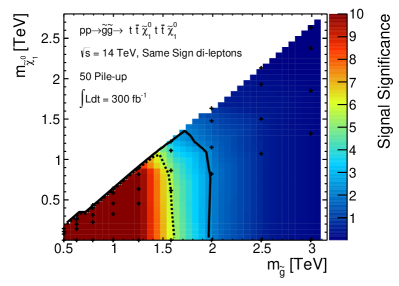
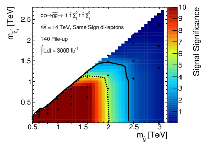
Refer to caption
Refer to caption
Refer to caption
Refer to caption
Figure 52: Results for the gluino-neutralino model with heavy flavor decays are given in the mχ~10subscript𝑚superscriptsubscript~𝜒10m_{\widetilde{\chi}_{1}^{0}} versus mg~subscript𝑚~𝑔m_{\widetilde{g}} plane. The solid [dotted] lines shows the expected 5σ5𝜎5\sigma discovery reach [95% confidence level upper limits] for gluino pair production. Mass points to the left/below the contours are expected to be probed at the 14 TeV14 TeV14{\text{ TeV}} LHC using 300 fb-1 [left] and 3000 fb-1 [right] of integrated luminosity. A 20% systematic uncertainty is assumed. The 300 fb1300superscript fb1300\text{ fb}^{-1} result on the left includes an average of 505050 pileup events; the3000 fb13000superscript fb13000\text{ fb}^{-1} result on the right includes an average of 140140140 pileup events. The results on the bottom do not include the effects of pileup.

Using the NLO gluino pair production cross section one can make a very naive estimate for the reach of a given collider. For example, we find that the choice of gluino mass which would yield 101010 SSDL events (accounting for the leptonic branching ratios) at 300 fb1300superscript fb1300\text{ fb}^{-1} (3000 fb1)3000superscript fb1\big{(}3000\text{ fb}^{-1}\big{)} is 2.3 TeV2.3 TeV2.3{\text{ TeV}} (2.8 TeV2.8 TeV2.8{\text{ TeV}}). This roughly corresponds to the maximal possible reach one could expect for a given luminosity using 14 TeV14 TeV14{\text{ TeV}} proton collisions.

Using a realistic simulation framework along with the search strategy employed here the 14 TeV14 TeV14{\text{ TeV}} 300 fb1300superscript fb1300\text{ fb}^{-1} limit is projected to be 1.9 TeV1.9 TeV1.9{\text{ TeV}} (corresponding to 73 events), and the 3000 fb13000superscript fb13000\text{ fb}^{-1} limit is projected to be 2.4 TeV2.4 TeV2.4{\text{ TeV}} (corresponding to 67 events). Finally, we note that the 14 TeV14 TeV14{\text{ TeV}} LHC with 3000 fb13000superscript fb13000\text{ fb}^{-1} could discover a gluino (with g~tt¯χ~10~𝑔𝑡¯𝑡superscriptsubscript~𝜒10\widetilde{g}\rightarrow t\,\overline{t}\,\widetilde{\chi}_{1}^{0}) as heavy as 2.0 TeV2.0 TeV2.0{\text{ TeV}} if the neutralino is massless. Note that due to the relatively weak cuts that can be placed on ETmisssuperscriptsubscript𝐸𝑇missE_{T}^{\mathrm{miss}}, the SSDL signal is robust against models with almost degenerate gluino and neutralino.

8.5   Analysis: 33 TeV

In this section, the signal regions are presented for the SSDL search at 33 TeV33 TeV33{\text{ TeV}} assuming 3000 fb13000superscript fb13000\text{ fb}^{-1}. Table 19 provides the values from an optimization for 300030003000 fb-1 of data. Also shown in these tables are number of events from the two dominant contributions to the background along with the total number of background events after cuts (including all contributions). When evaluating the gluino reach, we compute the signal efficiency after cuts for each signal region and use the one with the highest significance.

signal region BSM masses cuts backgrounds
SR1 mg~=997 GeVsubscript𝑚~𝑔997 GeVm_{\widetilde{g}}=997{\text{ GeV}} mχ~10=1 GeVsubscript𝑚superscriptsubscript~𝜒101 GeVm_{\widetilde{\chi}_{1}^{0}}=1{\text{ GeV}} ETmiss100 GeV;meff>1000 GeVformulae-sequencegreater-than-or-equivalent-tosuperscriptsubscript𝐸𝑇miss100 GeVsubscript𝑚eff1000 GeVE_{T}^{\mathrm{miss}}\gtrsim 100{\text{ GeV}};\quad m_{\text{eff}}>1000{\text{ GeV}} HT500 GeV;sym-MT240 GeVformulae-sequencegreater-than-or-equivalent-tosubscript𝐻𝑇500 GeVgreater-than-or-equivalent-tosym-subscript𝑀𝑇240 GeVH_{T}\gtrsim 500{\text{ GeV}};\quad\text{sym-}M_{T2}\gtrsim 40{\text{ GeV}} Njets>5;Nb>2formulae-sequencesubscript𝑁jets5subscript𝑁𝑏2N_{\text{jets}}>5;\quad N_{b}>2 tt¯𝑡¯𝑡t\,\overline{t} 19 di-boson 0.17 total 19.2
SR2 mg~=997 GeVsubscript𝑚~𝑔997 GeVm_{\widetilde{g}}=997{\text{ GeV}} mχ~10=641 GeVsubscript𝑚superscriptsubscript~𝜒10641 GeVm_{\widetilde{\chi}_{1}^{0}}=641{\text{ GeV}} ETmiss50 GeV;HT400 GeVformulae-sequencegreater-than-or-equivalent-tosuperscriptsubscript𝐸𝑇miss50 GeVgreater-than-or-equivalent-tosubscript𝐻𝑇400 GeVE_{T}^{\mathrm{miss}}\gtrsim 50{\text{ GeV}};\quad H_{T}\gtrsim 400{\text{ GeV}} meff700 GeVgreater-than-or-equivalent-tosubscript𝑚eff700 GeVm_{\text{eff}}\gtrsim 700{\text{ GeV}} Njets>5;Nb>2formulae-sequencesubscript𝑁jets5subscript𝑁𝑏2N_{\text{jets}}>5;\quad N_{b}>2 tt¯𝑡¯𝑡t\,\overline{t} 460 di-boson 9.2 total 470
SR3 mg~=1989 GeVsubscript𝑚~𝑔1989 GeVm_{\widetilde{g}}=1989{\text{ GeV}} mχ~10=1 GeVsubscript𝑚superscriptsubscript~𝜒101 GeVm_{\widetilde{\chi}_{1}^{0}}=1{\text{ GeV}} ETmiss500 GeV;HT1500 GeVformulae-sequencegreater-than-or-equivalent-tosuperscriptsubscript𝐸𝑇miss500 GeVgreater-than-or-equivalent-tosubscript𝐻𝑇1500 GeVE_{T}^{\mathrm{miss}}\gtrsim 500{\text{ GeV}};\quad H_{T}\gtrsim 1500{\text{ GeV}} meff2200 GeV;sym-MT2200 GeVformulae-sequencegreater-than-or-equivalent-tosubscript𝑚eff2200 GeVgreater-than-or-equivalent-tosym-subscript𝑀𝑇2200 GeVm_{\text{eff}}\gtrsim 2200{\text{ GeV}};\quad\text{sym-}M_{T2}\gtrsim 200{\text{ GeV}} Njets>7;Nb>2formulae-sequencesubscript𝑁jets7subscript𝑁𝑏2N_{\text{jets}}>7;\quad N_{b}>2 tt¯𝑡¯𝑡t\,\overline{t} 0.081 tri-boson 0.0062 total 0.087
SR4 mg~=1989 GeVsubscript𝑚~𝑔1989 GeVm_{\widetilde{g}}=1989{\text{ GeV}} mχ~10=1633 GeVsubscript𝑚superscriptsubscript~𝜒101633 GeVm_{\widetilde{\chi}_{1}^{0}}=1633{\text{ GeV}} ETmiss600 GeV;meff3000 GeVformulae-sequencegreater-than-or-equivalent-tosuperscriptsubscript𝐸𝑇miss600 GeVgreater-than-or-equivalent-tosubscript𝑚eff3000 GeVE_{T}^{\mathrm{miss}}\gtrsim 600{\text{ GeV}};\quad m_{\text{eff}}\gtrsim 3000{\text{ GeV}} Njets>7;Nb>2formulae-sequencesubscript𝑁jets7subscript𝑁𝑏2N_{\text{jets}}>7;\quad N_{b}>2 tt¯𝑡¯𝑡t\,\overline{t} 0.20 tj𝑡𝑗t\,j 0.035 total 0.26
SR5 mg~=3152 GeVsubscript𝑚~𝑔3152 GeVm_{\widetilde{g}}=3152{\text{ GeV}} mχ~10=1 GeVsubscript𝑚superscriptsubscript~𝜒101 GeVm_{\widetilde{\chi}_{1}^{0}}=1{\text{ GeV}} ETmiss1000 GeV;meff2000 GeVformulae-sequencegreater-than-or-equivalent-tosuperscriptsubscript𝐸𝑇miss1000 GeVgreater-than-or-equivalent-tosubscript𝑚eff2000 GeVE_{T}^{\mathrm{miss}}\gtrsim 1000{\text{ GeV}};\quad m_{\text{eff}}\gtrsim 2000{\text{ GeV}} sym-MT2300 GeVgreater-than-or-equivalent-tosym-subscript𝑀𝑇2300 GeV\text{sym-}M_{T2}\gtrsim 300{\text{ GeV}} Njets>7;Nb>2formulae-sequencesubscript𝑁jets7subscript𝑁𝑏2N_{\text{jets}}>7;\quad N_{b}>2 tri-boson 0.0062 total 0.0062
SR6 mg~=3152 GeVsubscript𝑚~𝑔3152 GeVm_{\widetilde{g}}=3152{\text{ GeV}} mχ~10=2796 GeVsubscript𝑚superscriptsubscript~𝜒102796 GeVm_{\widetilde{\chi}_{1}^{0}}=2796{\text{ GeV}} Njets>7;Nb>3formulae-sequencesubscript𝑁jets7subscript𝑁𝑏3N_{\text{jets}}>7;\quad N_{b}>3 tt¯𝑡¯𝑡t\,\overline{t} 2.9 tj𝑡𝑗t\,j 0.12 total 3.0
SR7 mg~=4968 GeVsubscript𝑚~𝑔4968 GeVm_{\widetilde{g}}=4968{\text{ GeV}} mχ~10=1 GeVsubscript𝑚superscriptsubscript~𝜒101 GeVm_{\widetilde{\chi}_{1}^{0}}=1{\text{ GeV}} ETmiss100 GeV;HT800 GeVformulae-sequencegreater-than-or-equivalent-tosuperscriptsubscript𝐸𝑇miss100 GeVgreater-than-or-equivalent-tosubscript𝐻𝑇800 GeVE_{T}^{\mathrm{miss}}\gtrsim 100{\text{ GeV}};\quad H_{T}\gtrsim 800{\text{ GeV}} meff1500 GeVgreater-than-or-equivalent-tosubscript𝑚eff1500 GeVm_{\text{eff}}\gtrsim 1500{\text{ GeV}} Njets>7;Nb>1formulae-sequencesubscript𝑁jets7subscript𝑁𝑏1N_{\text{jets}}>7;\quad N_{b}>1 tt¯𝑡¯𝑡t\,\overline{t} 390 di-boson 0.75 total 400
SR8 mg~=4968 GeVsubscript𝑚~𝑔4968 GeVm_{\widetilde{g}}=4968{\text{ GeV}} mχ~10=4612 GeVsubscript𝑚superscriptsubscript~𝜒104612 GeVm_{\widetilde{\chi}_{1}^{0}}=4612{\text{ GeV}} meff400 GeV;HT150 GeVformulae-sequencegreater-than-or-equivalent-tosubscript𝑚eff400 GeVgreater-than-or-equivalent-tosubscript𝐻𝑇150 GeVm_{\text{eff}}\gtrsim 400{\text{ GeV}};\quad H_{T}\gtrsim 150{\text{ GeV}} sym-MT2100 GeVgreater-than-or-equivalent-tosym-subscript𝑀𝑇2100 GeV\text{sym-}M_{T2}\gtrsim 100{\text{ GeV}} Njets>7;Nb>2formulae-sequencesubscript𝑁jets7subscript𝑁𝑏2N_{\text{jets}}>7;\quad N_{b}>2 tt¯𝑡¯𝑡t\,\overline{t} 1.6 tj𝑡𝑗t\,j 0.12 total 1.8
Table 19: The eight signal regions defined for the SSDL 333333 TeV 3000 fb13000superscript fb13000\text{ fb}^{-1} search. Also shown are the dominant two contributions to the background along with the total background after cuts, which also includes all subdominant backgrounds.

8.6   Results: 33 TeV

Using the signal regions outlined in the previous section, we determine the ability of the 333333 TeV LHC to probe this model in the SSDL channel. These results are presented in Fig. 53, where we show the 95%percent9595\% CL exclusion [solid line] and the 5σ5𝜎5\sigma discovery contours in the mχ~10subscript𝑚superscriptsubscript~𝜒10m_{\widetilde{\chi}_{1}^{0}} versus mg~subscript𝑚~𝑔m_{\widetilde{g}} plane. A 20%percent2020\% systematic uncertainty has been assumed for the background. Also shown in the right panel of this figure are the results without including pileup. The dominant effect of pileup on this analysis is that it can contaminate the lepton isolation cones, thereby reducing the signal strength. As we go to higher CM energy colliders the min bias events have higher pTsubscript𝑝𝑇p_{T} and begin to affect the lepton isolation more significantly. At 333333 TeV, in contrast with 141414 TeV, we find a small change in the overall reach and a substantial change in the reach for the high mass compressed region.
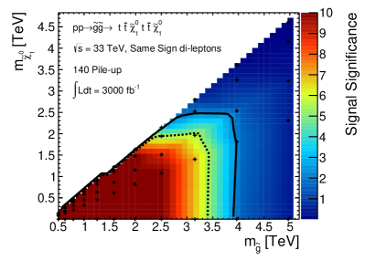
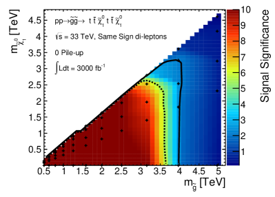
Refer to caption
Refer to caption
Figure 53: Results for the gluino-neutralino model with heavy flavor decays are given in the mχ~10subscript𝑚superscriptsubscript~𝜒10m_{\widetilde{\chi}_{1}^{0}} versus mg~subscript𝑚~𝑔m_{\widetilde{g}} plane. The solid [dotted] lines shows the expected 5σ5𝜎5\sigma discovery reach [95% CL upper limits] for gluino pair production. Mass points to the left/below the contours are expected to be probed at a 33 TeV33 TeV33{\text{ TeV}} proton collider using 3000 fb-1 of integrated luminosity. A 20% systematic uncertainty is assumed. For the figure on the left [right], an average of 140140140 [0]delimited-[]0[0] pileup events are included.

Using the NLO squark pair production cross section one can make a very naive estimate for the reach of a given collider. For example, we find that the choice of gluino mass which would yield 101010 SSDL events, i.e., appropriately accounting for the branching ratio, at 3000 fb13000superscript fb13000\text{ fb}^{-1} is 5.5 TeV5.5 TeV5.5{\text{ TeV}}. This roughly corresponds to the maximal possible reach one could expect for a given luminosity using 33 TeV33 TeV33{\text{ TeV}} proton collisions.

Using a realistic simulation framework along with the search strategy employed here the 33 TeV33 TeV33{\text{ TeV}} 3000 fb13000superscript fb13000\text{ fb}^{-1} limit is projected to be 4.0 TeV4.0 TeV4.0{\text{ TeV}} (corresponding to 243 events). Finally, we note that a 33 TeV33 TeV33{\text{ TeV}} proton collider with 3000 fb13000superscript fb13000\text{ fb}^{-1} could discover a gluino (with g~tt¯χ~10~𝑔𝑡¯𝑡superscriptsubscript~𝜒10\widetilde{g}\rightarrow t\,\overline{t}\,\widetilde{\chi}_{1}^{0}) as heavy as 3.4 TeV3.4 TeV3.4{\text{ TeV}} if the neutralino is massless. Note that due to the relatively weak cuts that can be placed on ETmisssuperscriptsubscript𝐸𝑇missE_{T}^{\mathrm{miss}}, the SSDL signal is robust against models with almost degenerate gluino and neutralino.

8.7   Analysis: 100 TeV

In this section, the signal regions are are presented for the SSDL search at 100 TeV100 TeV100{\text{ TeV}} assuming 3000 fb13000superscript fb13000\text{ fb}^{-1}. Table 20 provides the values from an optimization for 300030003000 fb-1 of data. Also shown in these tables are number of events from the two dominant contributions to the background along with the total number of background events after cuts (including all contributions). When evaluating the gluino reach, we compute the signal efficiency after cuts for each signal region and use the one with the highest significance.

signal region BSM masses cuts backgrounds
SR1 mg~=1995 GeVsubscript𝑚~𝑔1995 GeVm_{\widetilde{g}}=1995{\text{ GeV}} mχ~10=1 GeVsubscript𝑚superscriptsubscript~𝜒101 GeVm_{\widetilde{\chi}_{1}^{0}}=1{\text{ GeV}} ETmiss400 GeV;HT1500 GeVformulae-sequencegreater-than-or-equivalent-tosuperscriptsubscript𝐸𝑇miss400 GeVgreater-than-or-equivalent-tosubscript𝐻𝑇1500 GeVE_{T}^{\mathrm{miss}}\gtrsim 400{\text{ GeV}};\quad H_{T}\gtrsim 1500{\text{ GeV}} meff2000 GeV;sym-MT2100 GeVformulae-sequencegreater-than-or-equivalent-tosubscript𝑚eff2000 GeVgreater-than-or-equivalent-tosym-subscript𝑀𝑇2100 GeVm_{\text{eff}}\gtrsim 2000{\text{ GeV}};\quad\text{sym-}M_{T2}\gtrsim 100{\text{ GeV}} Njets>7;Nb>3formulae-sequencesubscript𝑁jets7subscript𝑁𝑏3N_{\text{jets}}>7;\quad N_{b}>3 tt¯𝑡¯𝑡t\,\overline{t} 0.53 total 0.53
SR2 mg~=1995 GeVsubscript𝑚~𝑔1995 GeVm_{\widetilde{g}}=1995{\text{ GeV}} mχ~10=1639 GeVsubscript𝑚superscriptsubscript~𝜒101639 GeVm_{\widetilde{\chi}_{1}^{0}}=1639{\text{ GeV}} ETmiss400 GeV;HT1200 GeVformulae-sequencegreater-than-or-equivalent-tosuperscriptsubscript𝐸𝑇miss400 GeVgreater-than-or-equivalent-tosubscript𝐻𝑇1200 GeVE_{T}^{\mathrm{miss}}\gtrsim 400{\text{ GeV}};\quad H_{T}\gtrsim 1200{\text{ GeV}} meff2000 GeV;sym-MT2100 GeVformulae-sequencegreater-than-or-equivalent-tosubscript𝑚eff2000 GeVgreater-than-or-equivalent-tosym-subscript𝑀𝑇2100 GeVm_{\text{eff}}\gtrsim 2000{\text{ GeV}};\quad\text{sym-}M_{T2}\gtrsim 100{\text{ GeV}} Njets>7;Nb>3formulae-sequencesubscript𝑁jets7subscript𝑁𝑏3N_{\text{jets}}>7;\quad N_{b}>3 tt¯𝑡¯𝑡t\,\overline{t} 0.53 total 0.53
SR3 mg~=3981 GeVsubscript𝑚~𝑔3981 GeVm_{\widetilde{g}}=3981{\text{ GeV}} mχ~10=1 GeVsubscript𝑚superscriptsubscript~𝜒101 GeVm_{\widetilde{\chi}_{1}^{0}}=1{\text{ GeV}} ETmiss1200 GeV;HT3500 GeVformulae-sequencegreater-than-or-equivalent-tosuperscriptsubscript𝐸𝑇miss1200 GeVgreater-than-or-equivalent-tosubscript𝐻𝑇3500 GeVE_{T}^{\mathrm{miss}}\gtrsim 1200{\text{ GeV}};\quad H_{T}\gtrsim 3500{\text{ GeV}} meff4500 GeV;sym-MT2350 GeVformulae-sequencegreater-than-or-equivalent-tosubscript𝑚eff4500 GeVgreater-than-or-equivalent-tosym-subscript𝑀𝑇2350 GeVm_{\text{eff}}\gtrsim 4500{\text{ GeV}};\quad\text{sym-}M_{T2}\gtrsim 350{\text{ GeV}} Njets>7;Nb>2formulae-sequencesubscript𝑁jets7subscript𝑁𝑏2N_{\text{jets}}>7;\quad N_{b}>2 tt¯𝑡¯𝑡t\,\overline{t} 0.60 total 0.60
SR4 mg~=3981 GeVsubscript𝑚~𝑔3981 GeVm_{\widetilde{g}}=3981{\text{ GeV}} mχ~10=3625 GeVsubscript𝑚superscriptsubscript~𝜒103625 GeVm_{\widetilde{\chi}_{1}^{0}}=3625{\text{ GeV}} ETmiss1200 GeV;HT4000 GeVformulae-sequencegreater-than-or-equivalent-tosuperscriptsubscript𝐸𝑇miss1200 GeVgreater-than-or-equivalent-tosubscript𝐻𝑇4000 GeVE_{T}^{\mathrm{miss}}\gtrsim 1200{\text{ GeV}};\quad H_{T}\gtrsim 4000{\text{ GeV}} meff5000 GeVgreater-than-or-equivalent-tosubscript𝑚eff5000 GeVm_{\text{eff}}\gtrsim 5000{\text{ GeV}} Njets>7;Nb>2formulae-sequencesubscript𝑁jets7subscript𝑁𝑏2N_{\text{jets}}>7;\quad N_{b}>2 tt¯𝑡¯𝑡t\,\overline{t} 0.85 tW𝑡𝑊t\,W 0.14 total 1.0
SR5 mg~=7944 GeVsubscript𝑚~𝑔7944 GeVm_{\widetilde{g}}=7944{\text{ GeV}} mχ~10=1 GeVsubscript𝑚superscriptsubscript~𝜒101 GeVm_{\widetilde{\chi}_{1}^{0}}=1{\text{ GeV}} ETmiss800 GeV;HT3000 GeVformulae-sequencegreater-than-or-equivalent-tosuperscriptsubscript𝐸𝑇miss800 GeVgreater-than-or-equivalent-tosubscript𝐻𝑇3000 GeVE_{T}^{\mathrm{miss}}\gtrsim 800{\text{ GeV}};\quad H_{T}\gtrsim 3000{\text{ GeV}} meff5000 GeVgreater-than-or-equivalent-tosubscript𝑚eff5000 GeVm_{\text{eff}}\gtrsim 5000{\text{ GeV}} Njets>7;Nb>2formulae-sequencesubscript𝑁jets7subscript𝑁𝑏2N_{\text{jets}}>7;\quad N_{b}>2 tt¯𝑡¯𝑡t\,\overline{t} 3.6 tW𝑡𝑊t\,W 0.20 total 3.8
SR6 mg~=7944 GeVsubscript𝑚~𝑔7944 GeVm_{\widetilde{g}}=7944{\text{ GeV}} mχ~10=7588 GeVsubscript𝑚superscriptsubscript~𝜒107588 GeVm_{\widetilde{\chi}_{1}^{0}}=7588{\text{ GeV}} HT400 GeV;meff800 GeVformulae-sequencegreater-than-or-equivalent-tosubscript𝐻𝑇400 GeVgreater-than-or-equivalent-tosubscript𝑚eff800 GeVH_{T}\gtrsim 400{\text{ GeV}};\quad m_{\text{eff}}\gtrsim 800{\text{ GeV}} Njets>7;Nb>2formulae-sequencesubscript𝑁jets7subscript𝑁𝑏2N_{\text{jets}}>7;\quad N_{b}>2 tt¯𝑡¯𝑡t\,\overline{t} 8100 tW𝑡𝑊t\,W 190 total 8300
SR7 mg~=15944 GeVsubscript𝑚~𝑔15944 GeVm_{\widetilde{g}}=15944{\text{ GeV}} mχ~10=1 GeVsubscript𝑚superscriptsubscript~𝜒101 GeVm_{\widetilde{\chi}_{1}^{0}}=1{\text{ GeV}} ETmiss500 GeV;HT4000 GeVformulae-sequencegreater-than-or-equivalent-tosuperscriptsubscript𝐸𝑇miss500 GeVgreater-than-or-equivalent-tosubscript𝐻𝑇4000 GeVE_{T}^{\mathrm{miss}}\gtrsim 500{\text{ GeV}};\quad H_{T}\gtrsim 4000{\text{ GeV}} meff6000 GeVgreater-than-or-equivalent-tosubscript𝑚eff6000 GeVm_{\text{eff}}\gtrsim 6000{\text{ GeV}} Njets>5;Nb>1formulae-sequencesubscript𝑁jets5subscript𝑁𝑏1N_{\text{jets}}>5;\quad N_{b}>1 tt¯𝑡¯𝑡t\,\overline{t} 45 single boson 1.8 total 50
SR8 mg~=15944 GeVsubscript𝑚~𝑔15944 GeVm_{\widetilde{g}}=15944{\text{ GeV}} mχ~10=15588 GeVsubscript𝑚superscriptsubscript~𝜒1015588 GeVm_{\widetilde{\chi}_{1}^{0}}=15588{\text{ GeV}} HT200 GeV;meff400 GeVformulae-sequencegreater-than-or-equivalent-tosubscript𝐻𝑇200 GeVgreater-than-or-equivalent-tosubscript𝑚eff400 GeVH_{T}\gtrsim 200{\text{ GeV}};\quad m_{\text{eff}}\gtrsim 400{\text{ GeV}} sym-MT2100 GeVgreater-than-or-equivalent-tosym-subscript𝑀𝑇2100 GeV\text{sym-}M_{T2}\gtrsim 100{\text{ GeV}} Njets>5;Nb>2formulae-sequencesubscript𝑁jets5subscript𝑁𝑏2N_{\text{jets}}>5;\quad N_{b}>2 tt¯𝑡¯𝑡t\,\overline{t} 2200 tW𝑡𝑊t\,W 16 total 2200
Table 20: The eight signal regions defined for the SSDL 100100100 TeV 3000 fb13000superscript fb13000\text{ fb}^{-1} search. Also shown are the dominant two contributions to the background along with the total background after cuts, which also includes all subdominant backgrounds.

8.8   Results: 100 TeV

Using the signal regions outlined in the previous section, we determine the ability of the 100100100 TeV LHC to probe this model in the SSDL channel. These results are presented in Fig. 54, where we show the 95%percent9595\% CL exclusion [solid line] and the 5σ5𝜎5\sigma discovery contours in the mχ~10subscript𝑚superscriptsubscript~𝜒10m_{\widetilde{\chi}_{1}^{0}} versus mg~subscript𝑚~𝑔m_{\widetilde{g}} plane. A 20%percent2020\% systematic uncertainty has been assumed for the background. Also shown in the right panel of this figure are the results without including pileup. The dominant effect of pileup on this analysis is that it can contaminate the lepton isolation cones, thereby reducing the signal strength. As we go to higher CM energy colliders the min bias events have higher pTsubscript𝑝𝑇p_{T} and begin to affect the lepton isolation more significantly. At 100100100 TeV, this effect is significant enough to decrease the limits on the gluino mass in this analysis by almost 1 TeV1 TeV1{\text{ TeV}}. Note that the lepton isolation cuts were not optimized for the higher pile-up and CM energy environments in this study; an interesting direction for future work would be to study how this issue can be ameliorated.
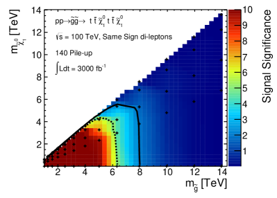
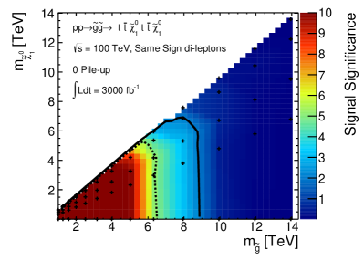
Refer to caption
Refer to caption
Figure 54: Results for the gluino-neutralino model with heavy flavor decays are given in the mχ~10subscript𝑚superscriptsubscript~𝜒10m_{\widetilde{\chi}_{1}^{0}} versus mg~subscript𝑚~𝑔m_{\widetilde{g}} plane. The solid [dotted] lines shows the expected 5σ5𝜎5\sigma discovery reach [95% confidence level upper limits] for gluino pair production. Mass points to the left/below the contours are expected to be probed at a 100 TeV100 TeV100{\text{ TeV}} proton collider using 3000 fb-1 of integrated luminosity. A 20% systematic uncertainty is assumed. For the figure on the left [right], an average of 140140140 [0]delimited-[]0[0] pileup events are included.

Using the NLO gluino pair production cross section one can make a very naive estimate for the reach of a given collider. For example, we find that the choice of gluino mass which would yield 101010 SSDL events at 3000 fb13000superscript fb13000\text{ fb}^{-1} is 12.7 TeV12.7 TeV12.7{\text{ TeV}}. This roughly corresponds to the maximal possible reach one could expect for a given luminosity using 100 TeV100 TeV100{\text{ TeV}} proton collisions.

Using a realistic simulation framework along with the search strategy employed here the 100 TeV100 TeV100{\text{ TeV}} 3000 fb13000superscript fb13000\text{ fb}^{-1} limit is projected to be 8.8 TeV8.8 TeV8.8{\text{ TeV}} (corresponding to 224 events). Finally, we note that a 100 TeV100 TeV100{\text{ TeV}} proton collider with 3000 fb13000superscript fb13000\text{ fb}^{-1} could discover a gluino (with g~tt¯χ~10~𝑔𝑡¯𝑡superscriptsubscript~𝜒10\widetilde{g}\rightarrow t\,\overline{t}\,\widetilde{\chi}_{1}^{0}) as heavy as 6.4 TeV6.4 TeV6.4{\text{ TeV}} if the neutralino is massless. Note that due to the relatively weak cuts that can be placed on ETmisssuperscriptsubscript𝐸𝑇missE_{T}^{\mathrm{miss}}, the SSDL signal is robust against models with almost degenerate gluino and neutralino.

8.9   Comparing Colliders

The same-sign di-lepton signature of the gluino-neutralino model with heavy flavor decays provides a useful case study with which to compare the potential impact of different proton colliders. Due to theoretical motivation in the context of both natural SUSY and split SUSY models, this final state is a very important signature of new physics to consider. Figure 55 shows the 5σ5𝜎5\sigma discovery reach [95%percent9595\% CL exclusion] for two choices of integrated luminosity at 141414 TeV, along with the full data set assumed for 333333 and 100100100 TeV. At the LHC, a factor of 101010 increase in luminosity leads to an improved reach of roughly 500500500 GeV. Increasing the center-of-mass energy has a tremendous impact on the experimentally available parameter space, since now much heavier gluinos can be produced without relying on the tails of parton distributions to supply the necessary energy. Figure 55 makes a compelling case for investing in future proton colliders which can operate at these high energies.

Note that studying other final states for this decay channel was outside the scope of this project. In light of these results though, it would be interesting to see if an all hadronic search would lead to improvements in the projected limits, especially since lepton efficiencies are significantly affected at high CM energies by the pile-up conditions and the highly boosted top quarks, and similarly to veto τ𝜏\tau-tagged jets to further reduce W/Z𝑊𝑍W/Z+jets. In particular, when considering searches at a 100 TeV100 TeV100{\text{ TeV}} collider, it would be interesting to investigate the fat top jet signatures of this model with very heavy gluinos.
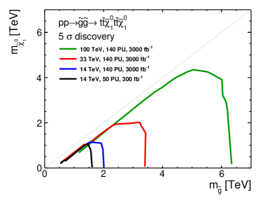
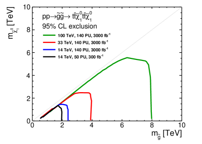
Refer to caption
Refer to caption
Figure 55: Results for the gluino-squark-neutralino model. The neutralino mass is taken to be 1 GeV1 GeV1{\text{ GeV}}. The left [right] panel shows the 5σ5𝜎5\,\sigma discovery reach [95%percent9595\% CL exclusion] for the four collider scenarios studied here. A 20%percent2020\% systematic uncertainty is assumed and pileup is included.

9 Outlook

Particle accelerators are one of the primary tools for experimentally investigating questions related to the microscopic properties of our Universe. Given the 20+limit-from2020+ year time scale required to build one of these machines, it is important to think carefully about their physics capabilities. A wide variety of studies are required for making informed decisions on the machine requirements such as center-of-mass energy, instantaneous and integrated luminosity; issues related to detailed detector design specifications must also be addressed.

This paper presents some of the first comprehensive comparisons between the upcoming 14 TeV14 TeV14{\text{ TeV}} run of the CERN Large Hadron Collider and future possible experiments (for other recent studies see [12, 13, 14, 15, 16, 17, 18, 19, 20, 21]). This includes a high-luminosity program at 14 TeV14 TeV14{\text{ TeV}}, and experiments that will collide protons at energies between 33similar-toabsent33\sim 33 and 100 TeVsimilar-toabsent100 TeV\sim 100{\text{ TeV}}. Our goal was to obtain the best limits possible with generic, signature-based searches that are not overly tuned to specific models.

We assessed the physics potential of these collider scenarios by performing analyses using Monte Carlo samples for signals and backgrounds with a realistic detector model. Results obtained with a fast detector simulation provide a complimentary estimate to a simple rescaling of existing limits, where the 888 TeV search strategies could be more sophisticated or involve more signal regions than the approaches taken here. Performing searches on Monte Carlo also provides insight into the impact of effects such as systematic uncertainties and pileup as a function of the center-of-mass energy.

In particular, we studied the reach for four SUSY Simplified Models whose experimental signatures are driven by the production of colored states. Three analysis strategies were employed in deriving these projections: a jets + ETmisssuperscriptsubscript𝐸𝑇missE_{T}^{\mathrm{miss}} analysis which optimized over HTsubscript𝐻𝑇H_{T} and ETmisssuperscriptsubscript𝐸𝑇missE_{T}^{\mathrm{miss}}, a mono-jet analysis with either an inclusive or exclusive jet requirement, and a same-sign di-lepton search. Table 21 shows the discovery potential [exclusion reach] for the different collider scenarios.

Simplified Model 14 TeV14 TeV14{\text{ TeV}} 300 fb1300superscript fb1300\text{ fb}^{-1} 14 TeV14 TeV14{\text{ TeV}} 3000 fb13000superscript fb13000\text{ fb}^{-1} 33 TeV33 TeV33{\text{ TeV}} 100 TeV100 TeV100{\text{ TeV}}
g~~𝑔\widetilde{g} - χ~10superscriptsubscript~𝜒10\widetilde{\chi}_{1}^{0} 1.9 TeV1.9 TeV1.9{\text{ TeV}} [2.3 TeV]delimited-[]2.3 TeV\big{[}2.3{\text{ TeV}}\big{]} 2.2 TeV2.2 TeV2.2{\text{ TeV}} [2.7 TeV]delimited-[]2.7 TeV\big{[}2.7{\text{ TeV}}\big{]} 5.0 TeV5.0 TeV5.0{\text{ TeV}} [5.8 TeV]delimited-[]5.8 TeV\big{[}5.8{\text{ TeV}}\big{]} 11 TeV11 TeV11{\text{ TeV}} [13.5 TeV]delimited-[]13.5 TeV\big{[}13.5{\text{ TeV}}\big{]}
light flavor decays
mχ~100similar-to-or-equalssubscript𝑚superscriptsubscript~𝜒100m_{\widetilde{\chi}_{1}^{0}}\simeq 0
g~~𝑔\widetilde{g} - χ~10superscriptsubscript~𝜒10\widetilde{\chi}_{1}^{0} 0.75 TeV0.75 TeV0.75{\text{ TeV}} [0.9 TeV]delimited-[]0.9 TeV\big{[}0.9{\text{ TeV}}\big{]} 0.9 TeV0.9 TeV0.9{\text{ TeV}} [1.0 TeV]delimited-[]1.0 TeV\big{[}1.0{\text{ TeV}}\big{]} 1.5 TeV1.5 TeV1.5{\text{ TeV}} [1.8 TeV]delimited-[]1.8 TeV\big{[}1.8{\text{ TeV}}\big{]} 4.6 TeV4.6 TeV4.6{\text{ TeV}} [5.5 TeV]delimited-[]5.5 TeV\big{[}5.5{\text{ TeV}}\big{]}
light flavor decays
mg~mχ~10similar-to-or-equalssubscript𝑚~𝑔subscript𝑚superscriptsubscript~𝜒10m_{\widetilde{g}}\simeq m_{\widetilde{\chi}_{1}^{0}}
q~~𝑞\widetilde{q} - χ~10superscriptsubscript~𝜒10\widetilde{\chi}_{1}^{0} 0.80 TeV0.80 TeV0.80{\text{ TeV}} [1.5 TeV]delimited-[]1.5 TeV\big{[}1.5{\text{ TeV}}\big{]} 0.9 TeV0.9 TeV0.9{\text{ TeV}} [1.7 TeV]delimited-[]1.7 TeV\big{[}1.7{\text{ TeV}}\big{]} 1.4 TeV1.4 TeV1.4{\text{ TeV}} [3.4 TeV]delimited-[]3.4 TeV\big{[}3.4{\text{ TeV}}\big{]} 2.4 TeV2.4 TeV2.4{\text{ TeV}} [8.0 TeV]delimited-[]8.0 TeV\big{[}8.0{\text{ TeV}}\big{]}
light flavor decays
mχ~100similar-to-or-equalssubscript𝑚superscriptsubscript~𝜒100m_{\widetilde{\chi}_{1}^{0}}\simeq 0
q~~𝑞\widetilde{q} - χ~10superscriptsubscript~𝜒10\widetilde{\chi}_{1}^{0} 0.45 TeV0.45 TeV0.45{\text{ TeV}} [0.65 TeV]delimited-[]0.65 TeV\big{[}0.65{\text{ TeV}}\big{]} 0.45 TeV0.45 TeV0.45{\text{ TeV}} [0.70 TeV]delimited-[]0.70 TeV\big{[}0.70{\text{ TeV}}\big{]} 0.80 TeV0.80 TeV0.80{\text{ TeV}} [1.3 TeV]delimited-[]1.3 TeV\big{[}1.3{\text{ TeV}}\big{]} 3.0 TeV3.0 TeV3.0{\text{ TeV}} [3.9 TeV]delimited-[]3.9 TeV\big{[}3.9{\text{ TeV}}\big{]}
light flavor decays
mq~mχ~10similar-to-or-equalssubscript𝑚~𝑞subscript𝑚superscriptsubscript~𝜒10m_{\widetilde{q}}\simeq m_{\widetilde{\chi}_{1}^{0}}
g~~𝑔\widetilde{g} - q~~𝑞\widetilde{q}- χ~10superscriptsubscript~𝜒10\widetilde{\chi}_{1}^{0} 2.7 TeV2.7 TeV2.7{\text{ TeV}} [2.8 TeV]delimited-[]2.8 TeV\big{[}2.8{\text{ TeV}}\big{]} 3.0 TeV3.0 TeV3.0{\text{ TeV}} [3.2 TeV]delimited-[]3.2 TeV\big{[}3.2{\text{ TeV}}\big{]} 6.6 TeV6.6 TeV6.6{\text{ TeV}} [6.8 TeV]delimited-[]6.8 TeV\big{[}6.8{\text{ TeV}}\big{]} 15.5 TeV15.5 TeV15.5{\text{ TeV}} [16 TeV]delimited-[]16 TeV\big{[}16{\text{ TeV}}\big{]}
light flavor decays
mg~mq~similar-to-or-equalssubscript𝑚~𝑔subscript𝑚~𝑞m_{\widetilde{g}}\simeq m_{\widetilde{q}} and mχ~100similar-to-or-equalssubscript𝑚superscriptsubscript~𝜒100m_{\widetilde{\chi}_{1}^{0}}\simeq 0
g~~𝑔\widetilde{g} - χ~10superscriptsubscript~𝜒10\widetilde{\chi}_{1}^{0} 1.6 TeV1.6 TeV1.6{\text{ TeV}} [1.9 TeV]delimited-[]1.9 TeV\big{[}1.9{\text{ TeV}}\big{]} 2.0 TeV2.0 TeV2.0{\text{ TeV}} [2.4 TeV]delimited-[]2.4 TeV\big{[}2.4{\text{ TeV}}\big{]} 3.4 TeV3.4 TeV3.4{\text{ TeV}} [3.9 TeV]delimited-[]3.9 TeV\big{[}3.9{\text{ TeV}}\big{]} 6.3 TeV6.3 TeV6.3{\text{ TeV}} [8.8 TeV]delimited-[]8.8 TeV\big{[}8.8{\text{ TeV}}\big{]}
heavy flavor decays
mχ~100similar-to-or-equalssubscript𝑚superscriptsubscript~𝜒100m_{\widetilde{\chi}_{1}^{0}}\simeq 0
Table 21: This table summarizes the expected discovery reach [95%percent9595\% CL limits] as computed using the search strategies employed in this study.

The results clearly demonstrate that these machines can have a substantial impact on our understanding of the parameter space of these models. They also address several big-picture questions when comparing colliders. In particular, it is possible to understand “how do analyses scale between these different machines?” by studying this work.

One example of how collider physics evolves as one moves to higher s𝑠\sqrt{s} is seen in the composition of the jets + ETmisssuperscriptsubscript𝐸𝑇missE_{T}^{\mathrm{miss}} backgrounds. This was most obvious in the g~qq¯χ10~𝑔𝑞¯𝑞superscriptsubscript𝜒10\widetilde{g}\rightarrow q\,\overline{q}\,\chi_{1}^{0} study of Sec. 3, where the dominant background was W/Z+jets𝑊𝑍jetsW/Z+\text{jets} at 14 TeV14 TeV14{\text{ TeV}}, but became tt¯𝑡¯𝑡t\,\overline{t} at 100 TeV100 TeV100{\text{ TeV}}. Another important lesson was illustrated in using the same-sign di-lepton approach to the g~tt¯χ10~𝑔𝑡¯𝑡superscriptsubscript𝜒10\widetilde{g}\rightarrow t\,\overline{t}\,\chi_{1}^{0} final state, where it was clear that the impact of pileup changed significantly between 14 TeV14 TeV14{\text{ TeV}} and 100 TeV100 TeV100{\text{ TeV}}. In particular, it is likely that lepton isolation requirements will need to evolve to cope with higher pTsubscript𝑝𝑇p_{T} objects and harder pileup interactions at high s𝑠\sqrt{s}.

There are many exciting opportunities for progress. This paper provides a concrete starting point for understanding the new physics potential of experiments that would collide protons at energies approaching the boundary of what humans can hope to achieve. By providing a quantitative analysis of several SUSY Simplified Models, these results help define many challenges and opportunities for future hadron colliders.

Acknowledgments

We thank Michael Peskin and Gavin Salam for helpful discussions. TC is supported by the US DoE under contract number DE-AC02-76SF00515 and was supported in part by the NSF under Grant No. PHYS-1066293 while enjoying the hospitality of the Aspen Center for Physics. AH is supported by the Alexander von Humboldt Foundation, Germany. KH is supported by an NSF Graduate Research Fellowship under Grant number DGE-0645962 and by the US DoE under contract number DE-AC02-76SF00515, and was partially supported by ERC grant BSMOXFORD no. 228169. SP was supported in part by the Department of Energy grant DE-FG02-90ER40546 and the FNAL LPC Fellowship. JGW is supported by the US DoE under contract number DE-AC02-76SF00515. The authors are supported by grants from the Department of Energy Office of Science, the Alfred P. Sloan Foundation and the Research Corporation for Science Advancement.

Appendix: Simulation Framework

This appendix is devoted to the details of our simulation procedure for the signal events. The publicly available Snowmass backgrounds [7] were used for all Standard Model Monte Carlo events.

Unless otherwise specified we applied the following systematic uncertainties to all analyses:

  • luminosity: 2.8%

  • PDF uncertainty: 5%

  • signal acceptance: 15%

  • background normalization: 20%

Parton level events were generated using Madgraph5 v1.5.10 [57]. All signals involve the pair production of SUSY particles and are matched using MLM matching up to 2 additional jets. The kTsubscript𝑘𝑇k_{T}-ordered shower scheme with a matching scale of qcut=xqcut=100 GeV100 GeV100{\text{ GeV}} was used. Note that we do not account for any possible inadequacies inherent in the current Monte Carlo technology, e.g. electroweak gauge bosons are not included in the shower.

The gluinos and squarks were treated as stable at the parton level. These events were subsequently decayed and showered using Pythia6 [58] and passed through the Delphes detector simulation [59] using the “Snowmass” detector parameter card [9]. Total production cross sections were computed at NLO using a modified version of Prospino v2.1 [60, 61, 62].

It proved to be advantageous to use a weighted event procedure. In particular, it was our goal to accurately model the tails of the distributions in the compressed region which is notoriously difficult to simulate. To this end we used a variation of the procedure developed for the Snowmass Standard Model background generation [7]. Since the only jets at the parton level were due to ISR, we could use generator level HTsubscript𝐻𝑇H_{T} variable which is built into Madgraph5. We will refer to cuts on this variable as htmin, htmax. This allowed us to bin events in “recoil” due to the presence of ISR — these are exactly the types of events which contribute in the compressed region.

In detail, the process for each parameter point is:

  1. 1.

    Compute the approximate differential cross section with respect to HTsubscript𝐻𝑇H_{T}. We run Madgraph in “survey” mode (using the command bin/madevent survey) while incrementing the htmin cut to determine the cross section as a function of this cut, σiσ(HT>htmini)subscript𝜎𝑖𝜎subscript𝐻𝑇subscripthtmin𝑖\sigma_{i}\equiv\sigma(H_{T}>\texttt{htmin}_{i}) with

    htmini=0n={0 GeV, 100 GeV, 200 GeV,}subscripthtmin𝑖0𝑛0 GeV100 GeV200 GeV\texttt{htmin}_{i=0\dots n}=\{0\mbox{ GeV},\,100\mbox{ GeV},\,200\mbox{ GeV},\dots\}

    We find that subsequent steps of 100 GeV provide an accurate enough characterization of the cross section for our purposes. We increase the cut until σi<1/subscript𝜎𝑖1\sigma_{i}<1/\mathcal{L} where \mathcal{L} is the luminosity for which good statistics are desired. The differential cross section is calculated from the differences:

    dσi=σi+1σi.dsubscript𝜎𝑖subscript𝜎𝑖1subscript𝜎𝑖\text{d}\sigma_{i}=\sigma_{i+1}-\sigma_{i}.
  2. 2.

    Determine bins of HTsubscript𝐻𝑇H_{T} for event generation. We define binα=1msubscriptbin𝛼1𝑚{\rm bin}_{\alpha=1\dots m} by htminαHT<htmaxαsubscripthtmin𝛼subscript𝐻𝑇subscripthtmax𝛼\texttt{htmin}_{\alpha}\leq H_{T}<\texttt{htmax}_{\alpha}. We choose bin edges based on a “weight fraction” x𝑥x with 0<x10𝑥10<x\leq 1 as follows:

    1. (a)

      The lower edge of the first bin is htmin1=0GeVsubscripthtmin10GeV\texttt{htmin}_{1}=0{\rm~{}GeV}.

    2. (b)

      The upper edge of the first bin htmax1subscripthtmax1\texttt{htmax}_{1} is chosen to be the smallest value such that σ1x×σtotsubscript𝜎1𝑥subscript𝜎tot\sigma_{1}\geq x\times\sigma_{\rm tot}.

    3. (c)

      The remaining upper bin edges htmaxα=2msubscripthtmax𝛼2𝑚\texttt{htmax}_{\alpha=2\dots m} are chosen similarly with each bin as small as possible such that

      σασ(htmaxα>HT>htminα)>x×σ(HT>htminα),subscript𝜎𝛼𝜎subscripthtmax𝛼subscript𝐻𝑇subscripthtmin𝛼𝑥𝜎subscript𝐻𝑇subscripthtmin𝛼\sigma_{\alpha}\equiv\sigma(\texttt{htmax}_{\alpha}>H_{T}>\texttt{htmin}_{\alpha})>x\times\sigma(H_{T}>\texttt{htmin}_{\alpha}), (3)

      with htminα=htmaxα1subscripthtmin𝛼subscripthtmax𝛼1\texttt{htmin}_{\alpha}=\texttt{htmax}_{\alpha-1}, where σ(bink)𝜎subscriptbin𝑘\sigma({\rm bin}_{k}) is the sum over dσidsubscript𝜎𝑖\text{d}\sigma_{i} for the range associated with bink.

    4. (d)

      The final bin is inclusive and determined by σ(binm)×<N/10𝜎subscriptbin𝑚𝑁10\sigma({\rm bin}_{m})\times\mathcal{L}<N/10, where N𝑁N is the total number of events to be generated in the final bin.

    Note that x=0.9𝑥0.9x=0.9 was used for this study.

  3. 3.

    Generate weighted events. We generate N5×104similar-to-or-equals𝑁5superscript104N\simeq 5\times 10^{4} generator-level events in each of the m𝑚m bins. For each bin separately, the events are showered, decayed, and matched in Pythia and reconstructed in Delphes. After matching, each bin has nkNsubscript𝑛𝑘𝑁n_{k}\leq N events and an associated matched cross section σLOmatchedsubscript𝜎LOmatched\sigma_{{\rm LO-matched}}.

References