Cosmic Emulation: Fast Predictions for the Galaxy Power Spectrum

Abstract

The halo occupation distribution (HOD) approach has proven to be an effective method for modeling galaxy clustering and bias. In this approach, galaxies of a given type are probabilistically assigned to individual halos in $N$-body simulations. In this paper, we present a fast emulator for predicting the fully nonlinear galaxy-galaxy auto and galaxy-dark matter cross power spectrum and correlation function over a range of freely specifiable HOD modeling parameters. The emulator is constructed using results from 100 HOD models run on a large $\Lambda$CDM $N$-body simulation, with Gaussian Process interpolation applied to a PCA-based representation of the galaxy power spectrum. The total error is currently $\sim 1$% in the auto correlations and $\sim 2$% in the cross correlations from $z=1$ to $z=0$, over the considered parameter range. We use the emulator to investigate the accuracy of various analytic prescriptions for the galaxy power spectrum, parametric dependencies in the HOD model, and the behavior of galaxy bias as a function of HOD parameters. Additionally, we obtain fully nonlinear predictions for tangential shear correlations induced by galaxy-galaxy lensing from our galaxy-dark matter cross power spectrum emulator.

All emulation products are publicly available at http://www.hep.anl.gov/cosmology/CosmicEmu/emu.html.

                                                                                                                                     ANL-HEP-PR-XX-XX

The Astrophysical Journal, submitted

1 Introduction

Measurements of galaxy clustering at large scales provide essential cosmological information, including key inputs to investigations of dark energy, the growth rate of structure, and neutrino mass. In particular, observations of two-point clustering statistics, such as the power spectrum and correlation function of galaxies obtained from large scale structure surveys, such as the Sloan Digital Sky Survey (SDSS)/BOSS (Baryon Oscillation Spectroscopic Survey), Two-degree Field Galaxy Redshift Survey, and WiggleZ, have been of particular significance (Pope et al., 2004; Tegmark et al., 2004, 2006; Cole et al., 2005; Eisenstein et al., 2005; Parkinson et al., 2012). Some of the strongest current constraints on the nature of dark energy have been derived from measurements of the Baryon Acoustic Oscillations (BAO) peak (e.g. Anderson et al., 2012, 2014) and redshift space distortions (RSDs) (e.g. Reid et al., 2012, 2014). Aside from the BAO scale, the amplitude and shape of the galaxy power spectrum and correlation function provide further cosmological information. In this case, it is desirable to include as many scales as is practical in the analysis, however, to do so requires that the nonlinear regime of structure formation be accurately modeled. As has been appreciated for quite some time, an essential difficulty is that galaxies are biased tracers of the underlying density field (Kaiser, 1984; Dekel & Rees, 1987). Because the nature of the bias is complex and often difficult to unravel, the underlying cosmological information cannot be straightforwardly extracted.

Modeling the distribution of galaxies remains an enduring problem in cosmology. $N$-body methods, while extremely successful in capturing the dark matter distribution at high resolution, do not incorporate the required baryonic physics for galaxies to emerge out of the large scale structure self-consistently. Furthermore, the positions of galaxies do not necessarily follow that of the dark matter, resulting in a nontrivial bias between statistical measurements of the clustering patterns between dark matter and galaxies. However, as mentioned above, accurate modeling of the nonlinear distribution of galaxies is crucial for extracting cosmological information from large scale structure surveys and understanding galaxy formation. Hydrodynamic simulations are still far from attaining the required degree of maturity needed to provide a complete first-principles understanding of galaxy formation. For these reasons, a number of phenomenological approaches – varying considerably in the amount of physical input – have been employed in the continuing quest to faithfully model galaxy clustering. (For a recent review, see Baugh 2013.)

The original, and simplest, approach is to assume a (nonlinear, scale-dependent) fitting function for the bias (defined, say, as the ratio between the galaxy and the linear or nonlinear matter power spectrum), combine this with clustering measurements, and marginalize over the free parameters. Like any such general approach, the problem is that the fitting form is not necessarily based on a physically correct model for galaxy formation, and if the form itself is not sufficiently flexible, this can lead to systematic errors in the determination of cosmological parameters. (See, e.g., a comparison of results from different bias models in Swanson et al. 2010; Parkinson et al. 2012.)

More detailed models for inferring the location of galaxies can be obtained by working at the level of dark matter-dominated halos and subhalos obtained from $N$-body simulations. These methods fall into three main categories: Halo Occupation Distribution (HOD) modeling, Subhalo/Halo Abundance Matching (S/HAM) and Semi-Analytic Models (SAMs). The HOD model is a probabilistic description that aims to reproduce the statistical distribution of target galaxies on average. This is achieved by populating dark matter halos with galaxies as a function of the halo mass. (We discuss HOD modeling more fully in Section 2.)

Halo abundance matching is an empirical procedure that involves rank ordering dark matter halos and subhalos in terms of a particular characteristic, such as mass or peak circular velocity during its accretion history (Vale & Ostriker, 2004; Conroy et al., 2006; Guo et al., 2010; Moster et al., 2010; Wetzel & White, 2010). Similarly, the galaxies are ordered according to an observable feature, say, luminosity. In this example, the most massive halo would be matched to the most luminous galaxy, the next most massive halo assigned the next most luminous galaxy, and so on, until no galaxies remain. This process ensures that the luminosity function is exactly reproduced by the synthetic galaxy catalog.

SAMs are the most complex, providing a simplified accounting of a large number of (baryonic) physical processes, embedded within $N$-body simulations. They include phenomenological prescriptions for galaxy formation and associated effects such as gas cooling, active galactic nuclei and supernova feedback, and star formation, based on the subhalo and halo formation history, e.g. (White & Frenk, 1991; Kauffmann, White, & Guiderdoni, 1993; Cole et al., 1994; Somerville & Primack, 1999; Benson et al., 2003; Baugh, 2006; Benson, 2010).

All of these more detailed methods can make predictions for galaxy clustering (and hence for bias), by using $N$-body simulations and some number of observational inputs to fix modeling parameters. The results for the galaxy power spectrum or correlation functions depend on the modeling parameters, as well as on cosmology. In many cases, it is not obvious exactly how the final answer depends on the interaction of these parameters, and an exhaustive sampling of parameter space by brute force can become computationally very expensive.

The general problem of efficiently sampling cosmological parameter space and building fast (essentially instantaneous), accuracy controlled, simulation-based predictors (“emulators”) for summary statistics has been addressed via the introduction of the Cosmic Calibration Framework (CCF). The CCF is based on efficient parameter sampling strategies coupled to Gaussian Process (GP) based interpolation and a Markov chain Monte Carlo (MCMC) sampler (Heitmann et al., 2006; Habib et al., 2007). The efficiency of the CCF for reproducing highly nonlinear observables is demonstrated in the Coyote (Heitmann et al., 2010, 2009; Lawrence et al., 2010) and extended Coyote (Heitmann et al., 2014) emulators for the matter power spectrum, accurate to 1% up to $k=1$ Mpc^-1 and 3-5% up to $k=8.6$ Mpc^-1, and an emulator for the halo concentration-mass ($c-M$) relation (Kwan et al., 2013), accurate to 3% at $z=0$.

This paper is concerned with providing a means for efficiently predicting galaxy 2-point statistics within the HOD model, using GP-based emulation. Our method presents a considerable advantage over algorithms that directly sample the dark matter halo catalogs (Neistein and Khochfar, 2012), because these involve a substantial computational overhead in terms of time and memory consumption. Moreover, the large scale information in the emulator is a product of several realizations of $N$-body simulations to reduce finite volume effects; this is not possible with a single catalogue as discussed in Neistein and Khochfar (2012). It is especially powerful because it can be run on a single processor and each run takes less than a second.

We adopt the HOD model as a first test case for emulation of galaxy based statistics because it is simple, yet flexible, and because it is the least demanding in terms of $N$-body simulation requirements. Using results from a high resolution simulation, we have populated the halos with galaxies from a sampling design with a 100 different HOD models, measuring the galaxy-galaxy and galaxy-dark matter power spectra from each model. This process is applied to six snapshots between $0\leq z\leq 1$ and we perform a linear interpolation to obtain additional power spectra at intermediate redshifts. The emulator is driven by a GP to return either a galaxy auto or cross power spectrum for arbitrary HOD models within the design. Sampling from the GP is a fast and accurate means of obtaining a nonlinear galaxy power spectrum without having to populate a halo catalog with a new HOD model each time. With the additional input of source and lens catalogs, the emulator can return the tangential shear $\left<\gamma_{t}(\theta)\right>$ or the excess surface density, $\Delta\Sigma(r)$.

In the following, we discuss our HOD approach, including the parameter choices, in Section 2. We describe the simulation underlying this work in Section 3 and provide some details on extracting the galaxy power spectra for the different HOD models from the simulation. Section 4 describes the emulator construction itself and the tests used for verifying its accuracy. Section 5 compares the performance of the emulator to a number of analytic halo models for the galaxy auto and cross power spectra. An initial set of scientific results based on the new emulator are reported in Sections 6 and 7, analyzing the dependence of the galaxy power spectrum on different HOD parameters and determining galaxy bias for different HOD models. In Section 8, we generalize the emulator to configuration space. In Section 9, we extend the galaxy-dark matter cross power spectrum emulator to calculate $\left<\gamma_{t}(\theta)\right>$ and $\Delta\Sigma(r)$. We conclude with a short discussion in Section 10.

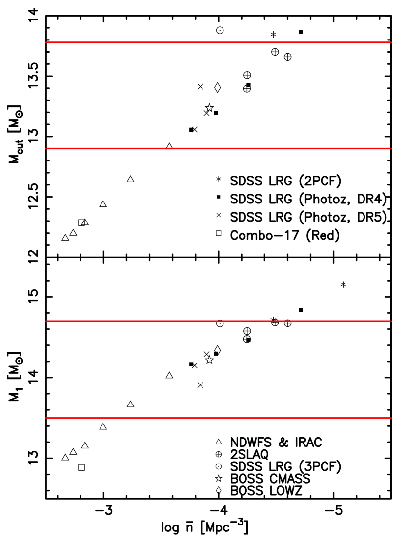
Figure 1: Range of the HOD emulator for $M_{cut}$ (top panel) and $M_{1}$ (bottom panel) compared to previous HOD analyses. The emulator covers the parameter space between the red lines. The survey data points are taken from Table A1 of Parejko et al. (2013) and include:  Zheng et al. (2009) [SDSS LRG (2PCF)],  Blake et al. (2008) [SDSS LRG (Photo-z, DR4)],  Padmanabhan et al. (2009) [SDSS LRG (Photo-z, DR5)], Phleps et al. (2006) [Combo-17 (Red)],  Brown et al. (2008) [NDWFS & IRAC], Wake et al. (2008) [2SLAQ], Kulkarni et al (2007) [SDSS LRG (3PCF)],  White et al. (2011) [BOSS CMASS] and  Parejko et al. (2013) [BOSS LOWZ].

2 The Halo Occupation Model

The HOD model (Kauffmann et al., 1997; Jing et al., 1998; Benson et al., 2000; Peacock & Smith, 2000; Seljak, 2000; Berlind & Weinberg, 2002) has evolved over time (cf. Zheng et al. 2005) into a straightforward method for associating galaxies with halos. The idea behind the HOD model is that every galaxy is required to be contained within a dark matter halo and galaxy populations are split into “centrals”, the bright main galaxy inside the halo, located at the halo center, and surrounding dimmer “satellite” galaxies. HOD models are calibrated against clustering observations of sets of target galaxies, allowing for an interpretation of the measurement in terms of a galaxy population model for halos. In this sense, the models are not predictive, and, in principle, have to be tuned to the galaxy population (defined, e.g., by color and luminosity) under consideration. (It is also not obvious that the simple assumption of the halo mass as the master variable is sufficiently accurate, due to halo assembly bias, as discussed in Gao et al. 2005.)

Despite the above caveats, the HOD approach has proven to be very successful when applied to large scale structure surveys, mostly to interpret their galaxy populations. These studies have informed us about the typical host halo mass and the ratio of satellite to central galaxies for a number of galaxy populations. The HOD model has been applied to both photometric and spectroscopic galaxy surveys, and hence galaxy types. These include Luminous Red Galaxies (LRGs), in the SDSS (Zehavi et al., 2004; Zehavi et al., 2005; Kulkarni et al, 2007; Blake et al., 2008; Zheng et al., 2009; Padmanabhan et al., 2009) and combined 2dF-SDSS LRG and QSO survey (2SLAQ) (Wake et al., 2008), red galaxies from the NOAO Deep Wide Field Survey (NDWFS), Spitzer IRAC Shallow Survey (Brown et al., 2008) and Combo-17 (Phleps et al., 2006) as well as CMASS (White et al., 2011) and LOWZ (Parejko et al., 2013) populations from BOSS.

In order to be specific, we adopt the HOD model of Zheng et al. (2009) for SDSS LRGs, although other models could easily have been considered. In this particular case, the average number of central and satellite galaxies, in a halo of mass $M$, is determined by the following equations:

$$\left<n_{\rm cen}\right>=\frac{1}{2}\;{\rm{erfc}}\left[\frac{\ln\left(M_{\rm cut}/M\right)}{\sqrt{2}\sigma}\right],$$ (1)

$$\left<n_{\rm sat}\right>=\left(\frac{M-\kappa M_{\rm cut}}{M_{1}}\right)^{\alpha}.$$ (2)

According to the HOD model, each halo must be assigned a probability of hosting a central galaxy based on the mass of the halo, with the sharpness of the cutoff mass determined by the parameter $\sigma$. If the halo is sufficiently massive to satisfy an additional cut in halo mass, imposed by $\kappa M_{\rm cut}$, then more galaxies are placed around the halo center as satellite galaxies; how many of these are inserted into the halo is controlled by the parameter $\alpha$. We assume that the number of satellite galaxies follows a Poisson distribution with mean $\left<n_{\rm sat}\right>$. The effect of these parameters on the mean number of galaxies assigned to each halo are illustrated in Figure 2 for two example HOD models. When calculating the contribution from satellite galaxies, instead of drawing dark matter particles from the halo at random based on the likelihood of hosting a galaxy, if a halo has been determined to host a satellite galaxy, each halo particle is assigned a weight according to the number of galaxies predicted by the HOD model. We do not weight halo particles unless the halo center also has a non-zero weight. This is done to reduce the level of shot noise in the power spectra. In this scheme, the halo center is given a weight of $\left<n_{\rm cen}\right>$, and each particle belonging to the halo has a weight of $\left<n_{\rm sat}\right>/N$, where $N$ is the total number of halo particles.

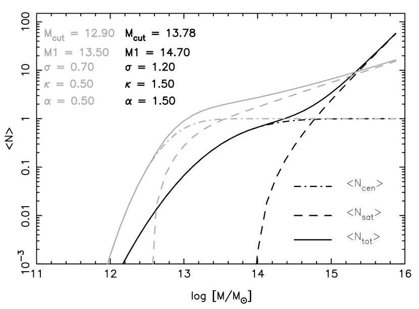
Figure 2: Mean number of central (dot-dashed) and satellite (dashed) galaxies per halo for two extreme HOD models at the edges of the prior range of the emulator. The average total number of galaxies per halo is shown as a solid curve. The two models shown have the lowest (grey) and highest (black) values in the HOD parameter space specified in Table 1.

The ranges of HOD parameters that we cover are given in Table 1 and illustrated in Figure 1 with respect to observational values obtained from large scale structure surveys. Figure 2 shows the values of $\left<n_{\rm cen}\right>$ and $\left<n_{\rm sat}\right>$ for the two HOD models at the extreme ends of the prior range. The emulator comfortably covers the HOD models used for the analysis of the recent CMASS BOSS results (White et al., 2011) as well as many SDSS LRG samples at certain redshifts and luminosity cuts.

Table 1: Prior Range of HOD Model Parameters

12.9	$\leq\log_{10}(M_{cut}[M_{\odot}])\leq$	13.78
13.5	$\leq\log_{10}(M_{1}[M_{\odot}])\leq$	14.7
0.5	$\leq\sigma\leq$	1.2
0.5	$\leq\kappa\leq$	1.5
0.5	$\leq\alpha\leq$	1.5

The parameter ranges of our emulator are motivated by the galaxy samples that we wish to study but ultimately limited by the mass resolution of our simulation; we only consider halos with a minimum mass cut set by a lower limit of 40 particles per halo, this in turn imposes a lower limit on $M_{\rm cut}$ and $\sigma$. While the smallest halos that we populate are actually less massive than the value of $M_{\rm cut}$ in that HOD model because $\sigma$ can substantially increase the value of $\left<n_{\rm cen}\right>$ for low mass halos, we have ensured that these limits are within the mass resolution of our simulation (discussed below) by setting an appropriately conservative lower limit on $M_{\rm cut}$. The upper limit is set mainly by statistical limitations due to the finite number of high mass halos in the simulation – a lower mass cut reduces the amount of noise in the power spectrum, and is in accordance with current and future galaxy surveys. Galaxy samples with excessively high $M_{\rm cut}$ and $M_{1}$ will have a low number density (high mass halos are rare) and as such there are few surveys that will target such galaxies. We have checked that the limits imposed in Table 1 will miss, at most, 1.6% of galaxies residing in halos below the mass resolution of the simulation. This translates to an error of $\sim$1% in the galaxy power spectrum as calculated from the halo model in the worse case scenario.

3 $N$-body Simulations

Our HOD catalogs are based on an $N$-body simulation with a box-size of $L=2100$ Mpc, 3200³ simulation particles and a cosmology similar to WMAP7: $\Omega_{m}=0.2648$ (including both cold dark matter and baryonic matter), $\Omega_{b}=0.0448,n_{s}=0.963,\sigma_{8}=0.8$, and $h=0.71$. This leads to a particle mass, $m_{p}=1.05\cdot 10^{10}$M_⊙. The force resolution was set to $\sim$9 kpc. Initial conditions were set with the Zel’dovich approximation, at $z_{\rm in}=200$. The simulation was performed using the HACC (Hardware/Hybrid Accelerated Cosmology Code) framework (Habib et al. 2009; Pope et al. 2010; Habib et al. 2012) on the Mira supercomputer at the Argonne Leadership Computing Facility.

To demonstrate the accuracy of our $N$-body simulation, we have shown the matter power spectrum in comparison to a smoothed average matter power spectrum in Figure 3, which was produced by averaging an additional 15 particle-mesh (PM) simulations combined with a theoretical matter power spectrum calculated from Resummed Perturbation Theory (RPT; Crocce & Scoccimarro (2006)), and then smoothed using a process convolution, according to the procedure outlined in Lawrence et al. (2010). Our RPT power spectra were calculated using the perturbation theory package, Copter (Carlson et al., 2009). The combination of the low resolution simulations reduces scatter from finite volume effects on the power spectrum on large scales. Note that the BAO feature has been enhanced relative to the simulation as a result of averaging over the additional realizations. We will later reuse these smoothed matter power spectra to obtain smoothed estimates of the galaxy power spectra. To avoid finite sampling errors on the very largest scales, we model the ratio of the matter power spectrum with respect to the galaxy-galaxy and galaxy-dark matter power spectra, rather than modeling each separately.

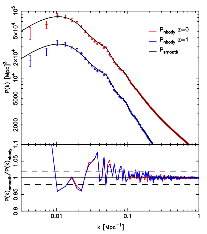
Figure 3: Matter power spectra measured from the $N$-body simulation at $z=0$ (red) and at $z=1$ (blue) with Poisson errors calculated from the number of counts in each bin in $k$. Smoothed matter power spectra obtained from an additional 16 PM runs and RPT (as described in Section 4.2) have also been shown for comparison. The lower panel shows the data presented as a ratio; the upper and lower horizontal lines indicate a 2% deviation.

Halos were identified with a Friends-of-Friends (FOF) algorithm (Einasto et al., 1984; Davis et al., 1985). This algorithm groups all particles that are joined to at least one other particle by a certain link length, $b$, as belonging to the same halo; approximately equivalent to requiring a minimum isodensity contour before an overdensity is considered a halo. Halo centers are assigned by identifying the gravitational potential minimum. We chose to use $b=0.168$, since this in rough correspondence with a spherical overdensity (SOD) mass of $M_{200}$, reduces halo over-linking, and is also consistent with other HOD analyses carried out on recent measurements, e.g. by White et al. (2011) and Parejko et al. (2013). The last feature allows for an easy comparison of results. The smallest halos we consider have at least 40 particles, leading to a halo mass of $\sim 4.2\cdot 10^{10}$M_⊙. At $z=0$, we have a total of $\sim 3.4\cdot 10^{7}$ halos in the simulation and there are $\sim$ 2000 halos with masses in excess of $9.55\cdot 10^{14}$M_⊙, ensuring good statistics for massive halos.

3.1 Measuring the Galaxy Auto and Cross Power Spectra from $N$-body Simulations

After having identified the halos in the simulations, the next step is the generation of galaxy catalogs following our HOD prescription outlined in Section 2. Varying the set of five HOD parameters introduced in Table 1, we generate 100 different models, arranged in a space-filling Symmetric Latin Hypercube design as explained in more detail in Section 4.1. For each of the 100 HOD models, the halo catalog is populated with galaxies from which we then measure a galaxy power spectrum. The power spectrum is defined as:

$$P(k)=\left<|\delta(k)|^{2}\right>,$$ (3)

where $\delta=(\rho-\bar{\rho})/\bar{\rho}$ and because we are interested in characterizing the clustering of galaxies, $\rho$ is the density of the galaxy field in the Universe. We use a Cloud in Cell (CIC) deposition on to a 10240³ grid to generate the density field, followed by a standard power spectrum estimation step using the Fast Fourier Transform (FFT). We then subtract the Poisson shot noise from each galaxy auto power spectrum; under our weighting scheme for the halo particles, this is defined as $\sum^{N}_{i=1}w_{i}/\sum^{N}_{i=1}w^{2}_{i}$, where $w$ is weight on each particle as determined by the HOD model. For the cross power spectrum, no weighting or shot noise subtraction is necessary, since the high resolution of the $N$-body simulation ensures that the shot noise contribution to the power spectrum is kept small.

4 Emulating the Galaxy Auto and Cross Power Spectra

Building a prediction scheme, or emulator, for the galaxy power spectrum, proceeds in three steps: (i) the design step, where we decide the HOD parameter settings at which to generate the power spectra, (ii) a smoothing step, where we take the resulting power spectra and filter discreteness noise caused by the finite number of galaxies in our catalogs, (iii) the interpolation step, where we build a GP model to generate predictions at new points in the HOD parameter space, leading to the final emulator. Next, we describe each of these steps in detail, followed by a rigorous testing procedure to verify the accuracy of our new emulator.

4.1 Design Strategy

The distribution of models in the five-dimensional HOD parameter space – the emulator design – is determined by a Symmetric Latin Hypercube to cover the maximum amount of parameter space with the fewest models. The technique for generating such a design is detailed in Heitmann et al. (2009) (including many references); the basic premise is that it is a space-filling design such that in any given two-dimensional projection of the full five-dimensional space, the models are approximately evenly sampled. The challenge is to determine a sufficiently large sample of models such that the target accuracy can be achieved without wasting computational time by oversampling.

Initially, we tried a set of 100 HOD models that span the range given in Table 1. The number of models chosen to cover the parameter space is determined by performing a series of tests in which we vary the number of design points used from 25, 50, to 100 and build a toy emulator for each set using halo model predictions for the HOD power spectrum as a proxy model (see Cooray & Sheth, 2002, for example) because these can be generated quickly. According to the halo model, the galaxy power spectrum is given by:

$$P_{gg}(k)=P^{1h}_{gg}(k)+P^{2h}_{gg}(k);$$ (4)

and

$$P^{1h}_{gg}=\int n(m)\frac{\left<N_{\rm gal}\left(N_{\rm gal}-1\right)|m\right>}{\bar{n}}|u(k|m)|^{2}\;dm$$ (5)

$$P^{2h}_{gg}=P_{L}\left[\int n(m)\;b(m)\frac{\left<N_{\rm gal}|m\right>}{\bar{n}}u(k|m)\;dm\right]^{2},$$ (6)

where $n(m)$ is the halo mass function, $\bar{n}$ is the mean density of galaxies and $u(k|m)$ is the dark matter mass profile in Fourier space, $P_{L}(k)$ is the linear matter power spectrum and $b(m)$ is the bias. Similarly, for the galaxy-dark matter cross power spectrum, we can write:

$$P_{gm}(k)=P^{1h}_{gm}(k)+P^{2h}_{gm}(k);$$ (7)

and

$$P^{1h}_{gm}=\frac{1}{\bar{n}}\int n(m)\frac{m}{\bar{\rho}}\left[|u(k|m)|^{2}\left<N_{\rm sat}|m\right>+u(k|m)\left<N_{\rm cen}|m\right>\right]dm$$ (8)

$$P^{2h}_{gm}=P_{L}\left[\int n(m)\;b(m)\frac{\left<N_{\rm gal}|m\right>}{\bar{n}}u(k|m)\;dm\right],$$ (9)

where $\bar{\rho}$ is the mean density of dark matter in the Universe.

Since there exist analytic prescriptions or fitting formulae for many of these terms, we can calculate these quantities much more readily compared to using galaxy catalogs from $N$-body simulations. The accuracy checks on these toy emulators are shown in Figure 4, in which we have selected five models not included in any of the designs and compared the predictions from each emulator to these. We found the proxy model easily achieves subpercent level accuracy with only 100 models. However, the response surface can be more complicated in the fully nonlinear case than in the simplified proxy model. In fact, we required 100 HOD models at redshifts, $z=0-0.66$, but 149 models for redshift $z=1$ to assure percent level accuracy in the final product. Unfortunately, the proxy model cannot fully account for the effect of shot noise in the galaxy power spectra and for the range of HOD models we considered, the shot noise was sufficiently different across the parameter space to require a closer sampling at high redshift where the halos are sparser. The estimate of the resultant accuracy of our emulator is verified by our later a posteriori tests (Section 4.4) carried out on the full emulator.

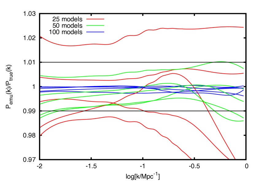
Figure 4: Accuracy test on the toy emulators built from halo model proxies. The aim is to estimate the number of models needed to cover the space of five HOD parameters with percent level accuracy. We built three emulators based on linear theory HOD models with 25 (red), 50 (green) and 100 (blue) design points and use these to predict the power spectrum of five models not included in the designs, which we denote $P_{\rm true}(k)$. The horizontal black lines denote our targeted accuracy of 1%.

4.2 Smoothing the power spectrum

In this section, we discuss the smoothing process used to convert the power spectra into noise-free estimates suitable for emulation. The galaxy auto and cross power spectra generated from the simulation contain measurement noise, because of finite volume effects and discrete sampling of Fourier modes. For the GP to function properly, we do not want to model noisy estimates of quantities as this would interfere with the ability of the GP to smoothly vary across the parameter space because of the random noise included with each function. Therefore we smooth the power spectra before they are used to condition the GP. We require that this effective filtering introduces errors of no more than $\sim$ 1% percent into the power spectrum measurement.

Our process for smoothing for the power spectrum proceeds in the following steps:

1. We measure the set of matter, galaxy-dark matter and galaxy-galaxy power spectra from the $N$-body simulation using the same sized FFT grids.

2. We take the ratio between the matter and the galaxy-galaxy and galaxy-dark matter power spectra to give the bias. This removes much of the scatter from finite volume effects, seen in Figure 3 on large scales, in the power spectra.

3. We then perform a basis spline on the binned power spectra. The bias is a simple enough function such that we can use a basis spline of order 4 with 10 coefficients evenly spaced throughout the $k$-range to capture the dependence of the bias on scale. The variance in the bias is sufficiently low such that the spline is able to capture the shape without much error as demonstrated in Figure 5.

4. The power spectra are then recovered by multiplying the bias with a smoothed estimate of the dark matter power spectrum. This is obtained from the same procedure that was used in Figure 5. In Lawrence et al. (2010), it was shown that the smoothing process, which uses additional information from the linear regime in the form of 15 low resolution simulations and perturbation theory, correctly captures the matter power spectrum to 1% accuracy.

In Figure 5, we show an example HOD galaxy-galaxy power spectrum with parameters, $M_{\rm cut}$ = 13.7086, $M_{1}$ = 13.4515, $\sigma$ = 0.6061, $\kappa$ = 0.9444 and $\alpha$ = 1.1364, chosen at random, after applying all the steps in the smoothing process. The results shown in the figure demonstrate that visually, there are no discernible defects in the galaxy power spectrum caused by our smoothing procedure and that the basis spline is sufficiently complex to fit the data points.

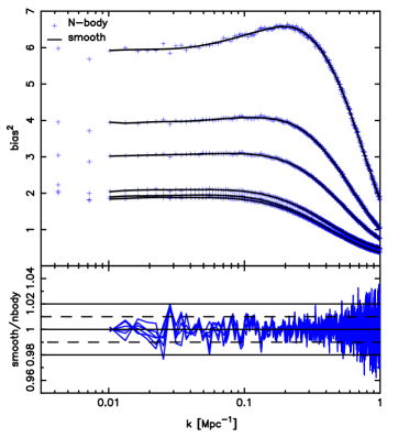
Figure 5: Example HOD model results obtained after applying the smoothing process at six redshifts. The top panel shows the ratio $P_{gg}/P_{m}$ measured from both the $N$-body simulation (blue crosses) and the smoothed HOD models (black curve). The bottom panel shows the ratio between the two, with dashed and solid lines indicating 1% and 2% error bands respectively.

4.3 Gaussian Process Modeling

Once the smoothed power spectra have been obtained at the design points, a Gaussian Process model is conditioned on these results, and can be interrogated to provide power spectrum predictions for any set of parameters chosen to lie within the prior range of Table 1.

The GP is a family of non-parametric, Gaussian distributed functions about a set of input points. The GP returns a function whose behavior is obliged to satisfy the input points at high accuracy. Our Gaussian model exists in parameter space, and not in $k-$space; i.e. the GP does not model each $k$ bin individually but rather the function as a whole over the entire parameter set. Overfitting is avoided by supplying a covariance function that regulates the complexity or “smoothness” of the function returned by the GP. This is achieved by controlling the relationship between each model in parameter space in terms of a distance metric. It is important that the underlying response surface mapped by the GP varies smoothly with the parameters – this requires the absence of sudden discontinuities as we move from one model to another with similar parameters. In most cosmological applications, this is not an issue, as most two-point statistics are quite well behaved when the underlying parameters are changed. However, we often do not know in advance the exact dependencies and degeneracies that exist in parameter space, particularly if the problem is nonlinear. For this reason, the form of the covariance function is parameterized with a set of hyperparameters. These are determined by maximizing the likelihood of these parameters given the simulation data, which we carry out via an MCMC process.

Our procedure for setting up the GP closely follows the method outlined in  Heitmann et al. (2006), Habib et al. (2007) and Heitmann et al. (2009). We have only briefly summarized the process here, because we are not so much concerned with the use of GPs for precision cosmology, but the application of GPs to the particular problem at hand. We refer the interested reader to the earlier papers for further details.

Once the GP is fully specified, we can draw a function, constrained to pass through the design points, at any point in the parameter space that satisfies the covariance function. This process is no more computationally expensive than calculating of the inverse of the covariance matrix with the new model included.

4.4 Testing the Emulator

In this section, we test the accuracy of the emulator by comparing the power spectrum generated by the emulator to HOD models directly sampled from our N-body simulation but not included in the conditioning of the GP. We apply the same smoothing process, described in Section 3.1, to these new HOD models. We repeat this test on both $P_{gg}(k)$ and $P_{gm}$ at each of the six redshift slices used to construct the emulator. In Figures 6, and 7, we show the results of these tests, demonstrating that the emulators are indeed accurate to $\sim 1$% and $\sim 2$% respectively, over the range $0.01\leq k\leq 1$ Mpc^-1. These accuracy limits are well below the accuracy requirement on $P_{gm}$ to extract HOD constraints from galaxy-galaxy lensing data for current experiments. Our test models are chosen at random to span the full range of parameters. Generally, the emulator should perform better near the center of the design and worse at the edges of the Latin hypercube, simply because there are a limited number of models that support the design edge. This is seen in some of the blue curves in Figure 6, particularly at $z=1$, which is poorly reproduced from $k\sim 0.8$ Mpc^-1 onwards because it lies on a corner of the design space and because galaxies from this HOD utilize the most massive halos i.e. $M_{\rm cut}=13.78$ and $M_{1}=14.7$ and hence require the most shot-noise subtraction.

Note that the errors in Figure 6 are percent level in the fully nonlinear case rather than below sub-percent level as in Figure 4 because the response surface is more complicated with nonlinear structure formation and there are additional contributions to the error budget in smoothing and shot noise.

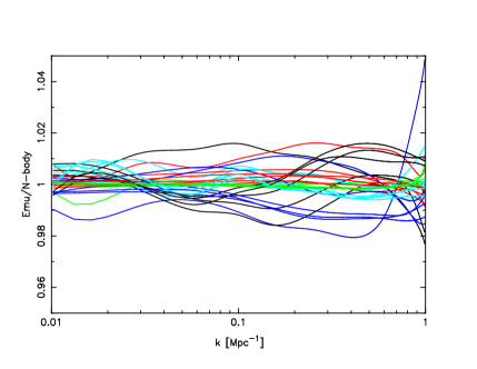
Figure 6: Accuracy test for $P_{gg}(k)$ : five HOD power spectra at each redshift are predicted by the emulator and compared to the same models directly measured from the $N$-body simulation not included in the original design. Each model is represented by a different color. The HOD power spectra returned by the emulator are within $\sim$ 1% of the smoothed $N$-body results on the scales $0.01\leq k\leq 1$ Mpc^-1 for the models tested.

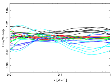
Figure 7: Accuracy test for $P_{gm}(k)$ at all redshifts. As in Figure 6, we test the emulator against five new HOD models drawn from the $N$-body simulation that were not included in the original design. Each color represents the same set of HOD parameters drawn from the within the parameter range at each of the six redshifts used to build the emulator.

5 Comparison to Analytic Models

We now compare the accuracy of our emulator to analytic predictions of the HOD power spectrum. These models are based on summing the 2-halo and 1-halo contributions to the galaxy power spectrum. The relevant equations for the most basic halo model (see, e.g., Cooray & Sheth 2002) are listed in Section 4.1 (Equations 4 – 6). The 2-halo term (Equation 5) describes galaxy pairs in two different halos, while the 1-halo term (Equation 6) arises from the galaxy pairs that occupy the same halo. There have been many revisions to this model and we consider two of the most popular, the Zheng (2004) and Tinker et al. (2005) models, which we will call Z04 and T05 respectively.

There are four ingredients to these models: the halo profile, the concentration-mass relation, the halo bias and the halo mass function. Whenever possible, we take the most recent fitting functions that are the most widely accepted in the literature to model these four quantities. We use an NFW profile to describe the distribution of galaxies in a halo. For the concentration-mass relation, we use Bhattacharya et al. (2013), which was calibrated on a $\Lambda$CDM cosmology that closely resembles our simulation in its $\Omega_{m}$ and $\sigma_{8}$ values.

To model the large scale halo bias, we use the following fitting function from Tinker et al. (2010)

$$b(\nu)=1-A\frac{\nu^{a}}{\nu^{a}+\delta_{c}^{a}}+B\nu^{b}+C\nu^{c}$$ (10)

where $A=1+0.24y\exp\left[-(4/y)^{4}\right]$, $a=0.44y-0.88$, $B=0.183$, $b=1.5$, $C=0.019+0.107y+0.19\exp\left[-(4/y)^{4}\right]$, $c=2.4$ and $y=\log_{10}\Delta$ and $\Delta=200$. For our FOF catalogs with $b=0.168$, $\Delta=200$ is the most appropriate background overdensity value considered in Tinker et al. (2010), who used halo catalogs identified with a SOD finder. Indeed, Tinker et al. (2010) report that a good agreement was found in the measured values of the large scale bias between FOF halo catalogs with $b=0.168$ and a SOD catalog of $\Delta=200$, despite the differences in the methodology and effects of aspherical FOF halo isodensity contours (Lukic et al, 2007). To this end, we also use the mass function from Tinker et al. (2008); although this is also calibrated on SOD halos, the normalization of the mass function is consistent with Equation 10 for the halo bias such that $\int b(\nu)n(\nu)\,d\nu=1$ and we would like to limit our analysis to only include model ingredients that are publicly available.

Our implementation of both the Z04 and T05 models use the same halo mass function, concentration-mass relation and the same expression for the large scale, linear halo bias. There are, however, two points on which the models differ; firstly the treatment of halo exclusion and secondly, the functional form assumed for the evolution of the halo bias as a function of scale. The Z04 model imposes halo exclusion by setting the upper integration limit, $M_{\rm lim}$, on the 2-halo term to avoid counting contributions from two overlapping halos. This is done by requiring $M_{\rm lim}=4/3\pi(r/2)^{3}\rho_{c}\Omega_{m}\Delta$, where $r$ is the radius of the halo, such that no other halo residing within half of the radius of a halo of mass, $M_{\rm lim}$, can be considered. T05 extends this halo exclusion model by allowing halos to be ellipsoidal and by modelling the distribution of the ratio of their major to minor axes. We can then calculate the effect of non-spherical halo alignments on the 2-halo term thusly:

$$P^{2h}_{gg}(k,r)=\frac{1}{\bar{n}^{\prime 2}}P_{m}(k)\int^{\infty}_{0}n(M_{1})\left<N_{\rm gal}|{M_{1}}\right>b(M_{1},r)u(k|M_{1})\;dM_{1}$$

$$\qquad\qquad\int^{\infty}_{0}n(M_{2})\left<N_{\rm gal}|{M_{2}}\right>b(M_{2},r)u(k|M_{2})p(y)\;dM_{2}$$ (11)

where $\bar{n}^{\prime}$ is the reduced number density and $p(y)=3y^{2}-2y^{3},y=(x-0.8)/0.29$ and is the probability of non-overlapping halos as calibrated from $N$-body simulations. The function $p(y)$ is bounded such that, when $y<0$, $p(y)=0$ and when $y>1$, $p(y)=1$. Equation 11 then requires a Hankel transform to remove the remaining dependence on scale and is reweighted thusly:

$$1+\xi^{2h}(r)={\left(\frac{\bar{n}^{\prime}}{\bar{n}}\right)}^{2}\left[1+\xi^{\prime 2h}(r)\right],$$ (12)

where $\xi^{\prime 2h}(r)$ is just the Hankel transform of $P^{2h}_{gg}(k,r)$ from Equation 11. Because the double integral in Equation 11 is time consuming to evaluate, we use the $\bar{n}^{\prime}$ matched limit as suggested in T05. This involves calculating the reduced number density as

$$\bar{n}^{\prime 2}=\int^{\infty}_{0}n(M_{1})\left<n_{\rm gal}|M_{1}\right>\;dM_{1}\int^{\infty}_{0}n(M_{2})\left<n_{\rm gal}|M_{2}\right>\;dM_{2},$$ (13)

then finding the value for the upper limit on the integral over halo mass that gives an equivalent number density to Equation 13 and replacing the $M_{lim}$ in the Z04 model with this value.

The halo bias in the T05 model is given by:

$$b^{2}(M,r)=b^{2}(M)\frac{\left[1+1.17\,\xi_{m}(r)\right]^{1.49}}{\left[1+0.69\,\xi_{m}(r)\right]^{2.09}}$$ (14)

where $b^{2}(M)$ is the expression in Equation 10 from Tinker et al. (2010) and $\xi_{m}$ is the matter correlation function. Unfortunately, the form of the scale dependence of the halo bias used in Z04 is not explicitly written out (it is only stated that it is calibrated to $N$-body simulations) and so we can only use the large scale asymptotic bias in the 2-halo term.

In Figure 8, we compare the Z04 and T05 models (solid and dotted-dashed, respectively), calculated using the halo model components described above, against our HOD emulator. We chose a random set of model parameters within our acceptable parameter range. On large scales, both power spectra agree to $\sim$10% (better than $\sim 5$% in the T05 model), then the Z04 model starts to deviate at $k\sim 0.06$ Mpc^-1, as the scale dependent bias becomes important and the contribution from the 1-halo term is inadequate at this scale to substantially increase the amplitude of the total power spectrum. In contrast, the T05 model remains accurate to $\sim 5\%$ down to $k\sim 0.17$ Mpc^-1. By allowing for non-spherical halos, there are additional contributions to the 2-halo term from halos that are fortuitously aligned along their minor axes and $P^{2h}(k)$ in the T05 model is boosted relative to the Z04 model. This results in the overall power spectrum having a better fit to the simulations. Note that the 1-halo contributions are the same for both models.

The evolution of the halo bias with scale makes a significant contribution in the T05 model in matching the amplitude of the power spectrum to the HOD emulator by boosting the linear halo bias. However, there are indications that the modeling of the scale dependent bias is not ideal. If we neglect the scale dependence in the halo bias in Equation 11, the T05 model is accurate to 10% down to $k\sim 0.3$ Mpc^-1 but the discrepancy between this version of the T05 model and the emulator is approximately constant with $k$. This suggests that the scale dependent bias would not be necessary (for this set of HOD parameters) if the large scale linear bias was better captured by Tinker et al. (2010). This implies that accurately characterizing the halo bias is a worthwhile endeavour if we are to improve the halo model.

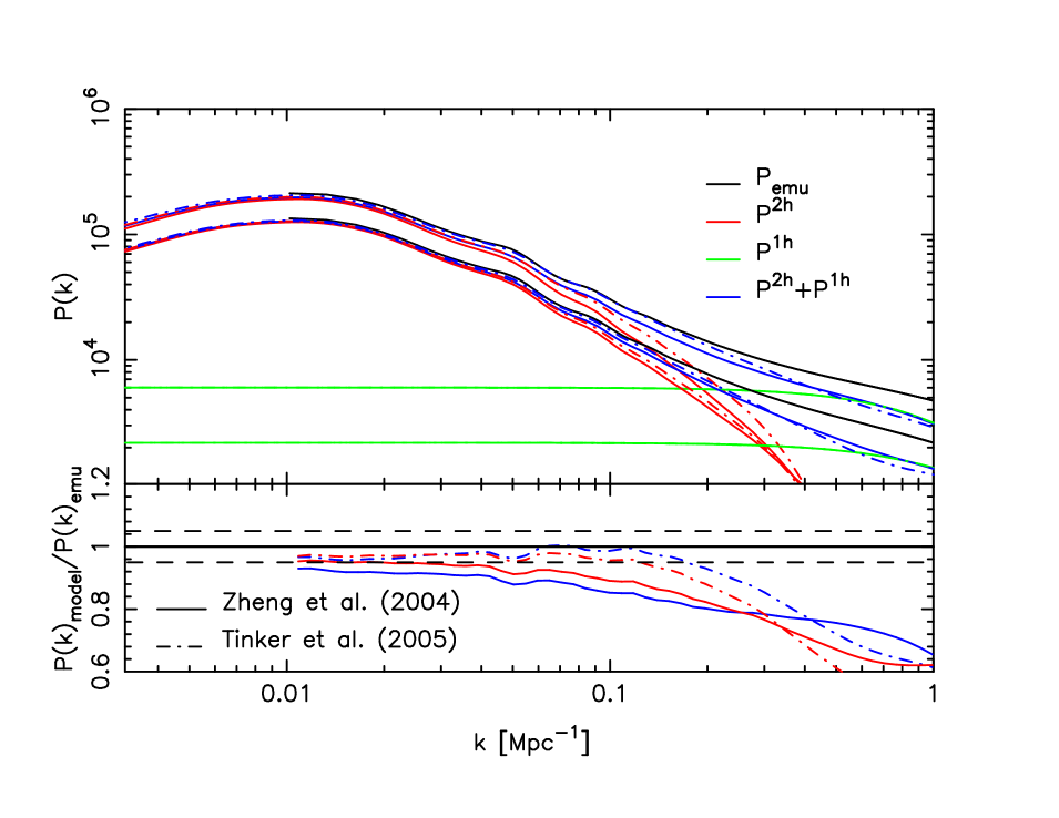
Figure 8: The auto and cross power spectra from the HOD emulator compared to the Zheng (2004) (Z04; solid) and Tinker et al. (2005) (T05; dotted-dashed) analytic models. We have split the total power spectrum from each of these models into their 2-halo (red) and 1-halo (green) components. The bottom panel shows the error in the analytic models compared to the emulator for the galaxy-dark matter cross power spectrum in red and the galaxy-galaxy power spectrum in blue. The large scale bias in the T05 model is reproduced quite well at the $\sim$ 5% level up to $k\sim 0.17$ Mpc^-1, but then there are deviations of up to 40% on smaller scales.

Past the quasi-linear scale, neither model can be trusted to derive accurate constraints on cosmology or the HOD parameters as the shape of the power spectrum is significantly biased at the 20-40% level. Unfortunately, this sort of halo model approach is only as good as its constituent fitting functions and the accuracy of these may be severely restrictive and dependant on the cosmology, volume, mass resolution etc. of the simulations used to calibrate them. Furthermore, the evaluation of these models is very slow, (the double integral in Equation 13 is particularly time consuming as is the transformation to configuration space for Equation 12); each model can take up to a minute to compute, compared to less than a second for the emulator.

Nonetheless, these models give an intuitive understanding of the HOD power spectrum via the halo model and its 2-halo and 1-halo contributions. Furthermore, while undoubtedly more accurate, by construction, the emulator can only operate within a certain parameter range, while, in principle, the halo model can be less restricted. Unfortunately, some of the ingredients of the halo model are also calibrated on $N$-body simulations, which can carry their own assumptions, such as the choice of a particle cosmology or in the implementation of a technique e.g. FOF versus SOD halo finding.

Figure 9: Emulated galaxy auto power spectrum at $z=0$. The five HOD parameters $M_{\rm cut},M_{1},\sigma,\kappa$ and $\alpha$ are varied. A single parameter is changed at a time in each panel, while the other four parameters are kept fixed at the midpoint of the parameter space. We divide the range of each parameter into ten evenly spaced bins, these are the values fed into the HOD emulator.

6 Parameter Sensitivities

Now that we are in possession of an HOD emulator, we can smoothly vary each HOD parameter in turn to investigate parametric degeneracies and other effects on the galaxy auto and cross power spectra. In Figure 9, we explore the effect of changing each parameter on the galaxy-galaxy auto power spectrum. We divide the parameter space into ten evenly spaced bins for each HOD parameter in turn, while keeping all the other parameters fixed at the center of the design, i.e. $M_{\rm cut}=13.35,M_{1}=13.8,\sigma=0.85,\kappa=1$ and $\alpha=1$. The resultant series of multiple power spectra are plotted in Figure 9.

The results shown in Figure 9 demonstrate that the parameters that most strongly affect the HOD power spectrum are $M_{cut}$ and $\alpha$, while $\kappa$ only minimally affects the power spectrum over our parameter range. The parameter, $M_{\rm cut}$, has the greatest influence in determining which halo will host a central galaxy. Since the majority of galaxies in our HOD models are centrals, it follows that $M_{\rm cut}$ has the greatest effect on the HOD power spectrum, especially on the linear bias.

In Figures 10 and 11, we have calculated $\partial\log P(k)/\partial\theta_{i}$ from the emulator as a function of wave number, (here $\theta_{i}=\{M_{\rm cut},M_{1},\sigma,\kappa,\alpha\}$) to demonstrate the degeneracies between the HOD parameters. The Fisher information matrix assess how well a parameter can be measured from a particular statistic and is defined as follows:

$$F_{ij}=-\left<\frac{\partial^{2}logf}{\partial\theta_{i}\partial\theta_{j}}\right>$$ (15)

From Tegmark (1997), we can approximate the Fisher matrix with

$$F_{ij}\approx 2\pi\int^{k_{\rm max}}_{k_{\rm min}}\left(\frac{\partial\log P(k)}{\partial\theta_{i}}\right)\left(\frac{\partial\log P(k)}{\partial\theta_{j}}\right)w(k)d\log k$$ (16)

Assuming the same survey window, $w(k)$, Figures 10 and 11, give an insight into how well these HOD parameters can be measured from the auto and cross power spectra respectively at two redshifts $z=0$ (grey) and $z=0.5$ (black).

Figure 10 shows that all the HOD parameters are degenerate on large scales, since they all show a similar relationship with $k$ up to $k=0.05$ Mpc^-1. This implies that they are all capable of shifting the linear, large scale asymptotic bias; but higher $M_{cut}$ and $\alpha$ values will increase the bias as the galaxy catalog will be populated from higher mass halos and more satellite galaxies, whereas increasing $M_{1}$ will decrease the bias, as a catalog with a higher $M_{1}$ will contain fewer satellite galaxies, if all other parameters are kept fixed. The parameter, $\sigma$, widens the mass cut on the central galaxies to accept more low mass halos and increasing $\sigma$ reduces the linear bias. At smaller scales up to $k=1$ Mpc^-1, $M_{\rm cut}$ affects the shape of the HOD power spectrum more strongly than any other parameter. At these scales, the power spectrum is still dominated by the two-halo term, so the additional satellite galaxies produced by having a larger value of $\alpha$ contributes less clustering than does $M_{\rm cut}$. As in Figure 9, $\kappa$ does very little to change the shape of the power spectrum. We have also investigated these relationships at $z=0.5$, as shown in Figure 10. By this redshift, the number of massive halos has been greatly reduced compared to $z=0$. This in turn reduces the influence of $M_{1}$ and $\alpha$ on the HOD power spectrum, which are only active parameters if $M\gtrsim 10^{14}$ $M_{\odot}$. Conversely, $\sigma$ and $M_{\rm cut}$ become more influential at higher redshift. We have also tried varying the central point in parameter space from which we calculate the derivatives of the parameter values. We found our conclusions to be qualitatively unchanged when the ‘midpoint’ is shifted to either edge of the parameter range, although the overall amplitudes of $\partial\log{\rm P}/\partial\theta_{i}$ may be more or less pronounced.

For the galaxy-dark matter cross power spectrum, Figure 11 shows that the dominant HOD parameter that determines its amplitude and shape is the mass cut off for the central galaxies, $M_{\rm cut}$. We can also expect to constrain, $\alpha$, which controls how many satellite galaxies to insert into each halo, much more readily than the typical mass of the halo hosting the galaxies, $M_{1}$, while $\sigma$ and $\kappa$ make very little difference to the shape and bias of the cross power spectrum.

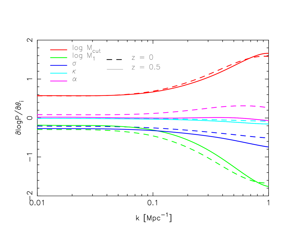
Figure 10: Derivatives of the galaxy-galaxy power spectrum with respect to the 5 HOD parameters, $\theta_{i}=\{M_{\rm cut}$ (red), $M_{1}$ (green), $\sigma$ (blue), $\kappa$ (cyan) and $\alpha$ (magenta) $\}$. We compute each partial derivative at the midpoint of the design at two redshifts, $z=0$ (dashed) and $z=0.5$ (solid).

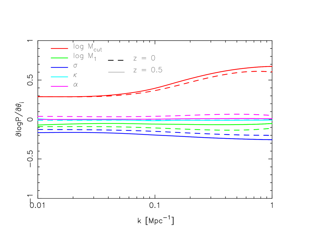
Figure 11: As in Figure 10, but for the galaxy-dark matter cross power spectrum. Note the change in scale on the y-axis.

Our results agree with Parejko et al. (2013), who found similar dependencies on the shape of the projected HOD correlation function, $w_{p}$, although their study probes much smaller scales than our HOD power spectrum emulator.

7 Nonlinear Bias

We now investigate the nonlinear galaxy bias with our HOD emulator. This is a difficult quantity to model analytically beyond the large scale, linear limit and our emulator offers a means of easily accessing nonlinear predictions for the galaxy bias. We define the galaxy bias as follows:

$$b(k)=\sqrt{\frac{P_{gg}(k)}{P_{m}(k)}},$$ (17)

where $P_{m}(k)$ can be chosen to be either the linear or nonlinear matter power spectrum, defining two notions of galaxy bias. In Figures 12 and 13, we show the evolution of the galaxy bias as a function of scale at $z=0$ and $z=1$, respectively. As in Figure 9, we have divided the parameter range into 10 bins, but in this section, we allow only $M_{cut}$ to change, since this is the parameter that the HOD power spectrum is most sensitive to, as shown previously in Section 6.

Figures 12 and 13 show that the nonlinearity of the bias increases with redshift when the HOD model is kept the same. The scale dependence of the bias in relation to the nonlinear matter power spectrum is quite moderate for the models with a low $M_{\rm cut}$ and is approximately linear until $k\sim 0.1-0.2$ Mpc^-1. The scale dependence is stronger at higher redshift, but this is because a galaxy catalog at this redshift with the same HOD parameters will contain rarer halos, i.e. there were much fewer $10^{15}$ M_⊙ halos at $z=1$ than $z=0$ and so these are more biased with respect to the matter density field.

In evaluating power spectra where the density field is reconstructed from mass points, there is an unavoidable shot noise contribution due to the finite mass resolution. At the highest $k$ values considered here, the shot noise in the matter power spectra is insignificant, because the particle Nyquist wave number in the simulation is sufficiently large (see Heitmann et al., 2010, for detailed evaluations and tests). A similar situation exists for the galaxy field: the preferential sampling of halos amongst the dark matter distribution introduces an element of shot noise in the galaxy power spectrum. We subtract a Poissonian shot noise term, proportional to $1/\bar{n}$ in keeping with current analyses of observational data, e.g Anderson et al. (2012). But halos are biased tracers that tend to follow the highest peaks of the dark matter density field, and by placing galaxies inside these, we have inherently chosen positions that are not a fair sample of the entire density field and so the generation of shot noise is not entirely a Poisson process in the galaxy power spectrum. It is important to note that the galaxy shot noise will make a substantial contribution to the bias shown in Figures 12 and 13 on small scales.

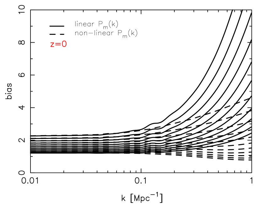
Figure 12: Nonlinear galaxy bias determined from the HOD emulator calculated using the linear $P_{m}(k)$ (solid) and nonlinear $P_{m}(k)$ (dashed) at $z=0$. We have varied $M_{\rm cut}$ between the maximum and minimum parameter ranges to produce 10 different curves. The other HOD parameters are kept constant at their midpoint values.

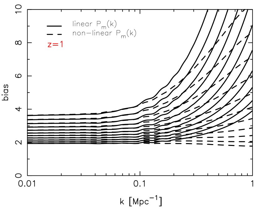
Figure 13: Galaxy bias, following Figure 12, but at $z=1$.

8 Configuration Space

We now consider the HOD power spectra in configuration space. Certain features, e.g. the baryon oscillations, are more prominent in configuration space than in Fourier space; additionally, the correlation function can be more readily measured from galaxy surveys than can the power spectrum, making the correlation function a more attractive quantity to model.

The correlation function is related to the power spectrum via the following transformation:

$$\xi(r)=\frac{1}{2\pi^{2}}\int k^{2}\;P(k)\;j_{0}(kr)\>dk,$$ (18)

where $j_{0}$ is the spherical Bessel function. Performing this integral is numerically challenging because of the highly oscillating integrand. Nonetheless, we attempt this brute force approach to obtain a reference correlation function which can be compared to more sophisticated methods. In order for the integral to converge, we introduce a smoothing term by multiplying the integrand with a damping factor of $\exp{(-k^{2}\sigma^{2})}$ where $\sigma=0.5$. We tried two other methods in addition to the brute force approach, a quadrature formula to approximate integrals over Bessel functions introduced by Ogata (2005) and applied to the correlation function by Szapudi et al. (2005) and FFTlog, an algorithm that performs Fast Fourier or Hankel transforms over logarithmically spaced intervals  (Hamilton, 2000).

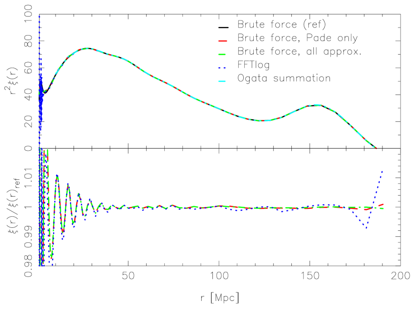
Figure 14: The matter correlation function produced by different schemes for calculating the Hankel transformation from Fourier space. This shows that the quadrature formula of Ogata (2005) and the extrapolations that we employ to calculate the correlation function from the power spectrum only introduces less than 1% error.

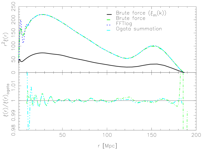
Figure 15: Similar to Figure 14 but now testing the Ogata (2005) integral, FFTlog (Hamilton, 2000) and brute force integration, using the HOD power spectrum emulator as input. The power spectrum has been extrapolated into both the linear and nonlinear regimes by a simple power law and using a Padé approximant respectively.

As shown in Ogata (2005), integrals involving Bessel functions such as the one that appears in Equation 18 can be approximated as:

$$\int f(x)J_{\nu}(x)\;dx$$

$$\approx\pi\sum_{n=1}^{k}w_{\nu k}f(\pi\psi_{\nu k}(hr_{\nu k})/h)J(\pi\psi_{\nu k}(hr_{\nu k})/h){\psi_{\nu k}}^{\prime}(hr_{\nu k})$$

(19)

where $\psi(x)=x\tanh[(\pi/2)\sinh(x)]$, $h$ is the step length of the integration, $w_{\nu k}(x)=Y_{\nu}(x)/J_{\nu+1}(x)$ and $r_{\nu}$ are the zeros of the Bessel function. For the correlation function, we want to consider $\nu=1/2$, since $j_{0}(x)=\sqrt{(\pi/2x)}J_{1/2}$. Two parameters, $h$, the step size, and $k$, the number of steps performed, control the accuracy of the integration. We use $h=1/150$ and $m=500$ and have verified that for $f(x)=1$, the integral is indeed equal to 1. We found that these parameters were a good compromise between accuracy and the time taken to calculate the sum in Equation 19. However, these two methods also require the power spectrum to be known over a large range of wavelengths, much larger than the range covered by the HOD emulator.

To extend the power spectrum to larger length scales, we use the smoothed matter power spectrum multiplied by the linear bias up to $k=0.001$ Mpc^-1 and beyond that, we match a simple power law extrapolation, $P(k)\propto k^{n}$, to the amplitude of the primordial power spectrum, where $n=0.963$.

The smaller scales are extended to $k=10^{3}$ Mpc^-1 with a scheme based on a Padé approximant, $R(x)$, which is a series approximation defined as $R_{[n,m]}(x)=\left(\sum^{n}_{i=0}a_{n}x^{n}\right)/\left(1+\sum^{m}_{i=1}b_{m}x^{m}\right)$ for constants, $a_{0},a_{1},...,a_{n}$, and $b_{1},b_{2},...b_{n}$. Fortunately, the behavior of the correlation function on the scales that we emulate is not affected too much by the power spectrum on these extremely large scales; we only require a smooth extrapolation that approaches zero as $k$ increases. We chose a Padé approximation of the form $R_{[0,m]}(k)=a_{0}/(1+b_{1}k+b_{2}k^{2})$, because the power spectrum appears to approach a power law, $k^{-2}$, on small scales. The constants $a_{0},b_{1},b_{2}$ are set by matching the function to $P(k)$ at three points at $k\approx 0.699,0.848,0.995$ Mpc^-1. Because the amplitude of the power spectrum rapidly approaches zero in the nonlinear regime, the correlation function is largely insensitive to the exact form used to extrapolate the power spectrum to small scales; we only require that it exists for the integral to converge. Nonetheless, in Figure 14, we check each of these assumptions in turn. We generate a power spectrum up to $k=10$ Mpc^-1 using the extended Coyote matter power spectrum emulator (Heitmann et al., 2014) and this is transformed into a correlation function via Equation 18 using a brute force integration. This acts as a reference (Figure 14; black) to which we can compare the effect of our extrapolation methods on the resultant correlation function. In Figure 14, we show two more correlation functions whose corresponding matter power spectrum was extrapolated to smaller scales using the Padé approximation (red) and additionally extended with a power law to model the linear regime (green). We also compare the methods proposed by Ogata (2005) (cyan) and Hamilton (2000) (dark blue). The bottom panel shows that the relative error as a result of making these assumptions compared to the brute force approach is less than 1%. In Figure 15, we demonstrate that this still holds for the galaxy power spectra produced by our emulator. However, we are only able to test the various prescriptions used to evaluate the Hankel transform in Equation 18 because the $k-$range of the emulator is not wide enough for the brute force method to work without some sort of extrapolation. The three methods that we consider in Figure 15 all yield results consistent to 1%.

9 Galaxy-Galaxy Lensing

We now demonstrate the usefulness of our emulator by applying our predictions for the galaxy-matter cross power spectrum to estimate the average tangential shear produced by galaxies residing in dark matter haloes. Galaxy-galaxy lensing involves the distortion of background galaxy images by the dark matter haloes of foreground galaxies. Because galaxy-galaxy lensing is concerned with probing the halo profile of galactic sized dark matter haloes, the HOD model is a natural candidate for modeling the distribution of galaxies on small scales. Indeed, some of the strongest constraints on small scale structure have been derived from applying the HOD model to observations of galaxy-galaxy lensing.

The tangential shear from galaxy-galaxy lensing is given by Moessner & Jain (1998); Guzik & Seljak (2001):

$$\left<\gamma_{t}(\theta)\right>=6\pi\Omega_{m}\int d\chi\,f_{\chi}(\chi^{\prime},\chi)\frac{n_{1}(\chi)}{a(\chi)}\int dk\,k\,P_{gm}(k,\chi)\,J_{2}(k,\theta,\chi),$$ (20)

where $f(\chi^{\prime},\chi)=\int d\chi^{\prime}n_{2}(\chi^{\prime})\frac{\chi(\chi-\chi^{\prime})}{\chi^{\prime}}$ is defined as the lens efficiency, $\chi$ is the comoving angular distance and $a$ is the scale factor. The normalized distributions of foreground (lens) and background (source) galaxies are given by $n_{1}(\chi)$ and $n_{2}(\chi)$ respectively.

Our emulator also calculates the excess surface density in the plane of the lensing potential, $\Delta\Sigma$ via the following equation:

$$\Delta\Sigma(R)=\Sigma_{crit}\left<\gamma_{t}(R)\right>,$$ (21)

where $\Sigma_{crit}=\frac{c^{2}}{4\pi G}\frac{D_{s}}{D_{l}D_{ls}}$ is the critical surface density and $D$ is the angular diameter distance in proper coordinates.

To evaluate the Hankel transform in Equation 20, it is necessary to extend the galaxy-dark matter power spectrum to smaller scales to allow the integral to converge. Again, we adopt the Padé approximation because this approach involves minimal assumptions about the high $k$ behaviour of the galaxy-dark matter cross power spectrum. This time, however, we add an additional exponential damping term to prevent the bias from becoming too large in the small scale regime. Another possible extension is to add a baryon model (such as $\propto<M>/R^{2}$ to represent the stellar contribution as additional lensing with a point mass) as in Velander et al. (2013) or model of sub-halo clustering with truncated NFW profiles as in Li et al. (2014) instead with additional fitted parameters.

In Figure 16, we show the dependence of the tangential shear, $\left<\gamma_{t}(\theta)\right>$, (grey) excess surface density, $\Delta\Sigma(r)$, on our five HOD parameters. By far, the mass cut on centrals, $M_{\rm cut}$, dominates all the other HOD parameters and we can only expect to constrain two parameters, $M_{\rm cut}$ and $M_{1}$ easily. This motivates a joint analysis involving another statistic such as $w(\theta)$ to break the degeneracy between the HOD parameters. Furthermore, Figure 16 suggests that these HOD parameters may be more readily constrained from $\left<\gamma_{t}(\theta)\right>$ than $\Delta\Sigma(r)$.

The use of our emulator removes the reliance on halo model based methods and provides a significantly more accurate estimate of the non-linear clustering in the large-$k$ regime as demonstrated in our comparisons with halo model in Section 5. In addition, the emulator is substantially faster at evaluating the cross galaxy-matter power spectrum than any of the analytic methods that we have considered. Using the emulator instead of an analytic model reduces the run time on a typical MCMC analysis with $\sim 10^{4}$ steps for convergence from $\sim$10 hours to $\sim$ 15 minutes on a single processor, since each evaluation of $\left<\gamma_{t}(\theta)\right>$ with the emulator saves about five seconds. The emulator will be applied to observations of $\left<\gamma_{t}(\theta)\right>$ and $\Delta\Sigma(r)$ to determine the HOD of galaxies in the sample (in prep). For this purpose, we have additionally built an emulator with an extended parameter range covering halos down to M${}_{\rm cut}\sim 10^{12.5}$M_⊙ with only an additional 50 models per redshift, at the cost of downgrading the accuracy of the power spectra to $\sim$ 5%. Fortunately, this is not an issue for current datasets. This allows our tool to be more robust against changes in galaxy samples. The nested design demonstrates the flexibility of the Cosmic Calibration Framework as a powerful tool for providing fast, nonlinear predictions for the purposes of deriving cosmological constraints from observations.

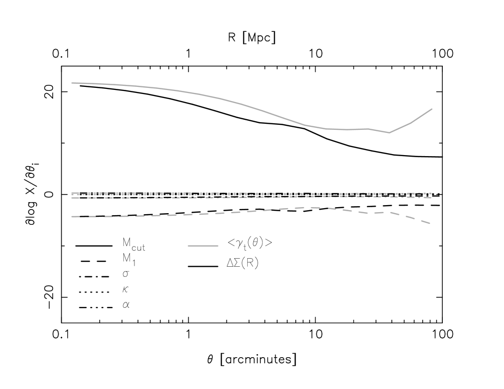
Figure 16: Derivatives of the averaged tangential shear $\left<\gamma_{t}(\theta)\right>$ (grey) and excess surface density, $\Delta\Sigma(r)$ (black) with respect to the 5 HOD parameters, $\theta_{i}=\{M_{\rm cut}$ (solid), $M_{1}$ (dashed), $\sigma$ (dotted-dashed), $\kappa$ (dotted) and $\alpha$ (dotted-dotted- dashed) $\}$. We assume a redshift range of $0.2<z<0.4$ for the sources and $0.5<z<1.3$ for the lens catalog and a redshift distribution typical of the Dark Energy Survey.

10 Conclusions

We present an emulator for an HOD-based galaxy-galaxy and galaxy-dark matter cross power spectra (and correlation functions) obtained from an $N$-body simulation. The emulator is accurate to $\sim$1% (auto) and $\sim$2% (cross) over the range $0.01\leq k\leq 1$ Mpc^-1 $(1\leq r\leq 180\;\rm{Mpc})$ from $0\leq z\leq 1$. Using our emulator, we explore the parameter degeneracies of the five-parameter HOD model of Zheng et al. (2009), finding significant degeneracies between the parameters on large scales. Changes in M_cut dominate both the shape and overall amplitude of the HOD power spectrum, while the parameter $\kappa$ has a very small effect. We show how the emulator can be used to extract scale-dependent galaxy bias. By comparing against the emulator results, we find that that analytic halo model predictions for the galaxy bias, such as that of Zheng (2004) and Tinker et al. (2005), while reasonably accurate at large length scales ($k<0.1$ Mpc^-1), cannot be used to derive accurate constraints on cosmology or the HOD parameters as the form of the resulting galaxy power spectrum is significantly biased at the 20-40% level at smaller length scales. We also extend the emulator to provide predictions for the averaged tangential shear, $\left<\gamma_{t}(\theta)\right>$ and excess surface density, $\Delta\Sigma(r)$, which are highly useful for obtaining the HOD of source galaxies from galaxy-galaxy lensing. We explore the parameter degeneracies in these statistics and find that the main parameter that affects the measurement of the shear is M_cut.

Emulation is a powerful technique for efficiently generating accurate models for highly nonlinear quantities in cosmology, such as the galaxy power spectrum. The emulator only requires a small number (100) of models to be directly computed from the halo catalog of an $N$-body simulation, following which each prediction from the emulator takes less than a second. This can substantially reduce the run time needed for an MCMC analysis where, in the current approach e.g. White et al. (2011); Parejko et al. (2013), the halo catalog and power spectrum are recomputed at each step. To facilitate use by the community, the emulator code has been publicly released.

Future plans to extend the emulator include the addition of cosmological parameters to the HOD parameter space and the modeling of redshift space distortions.

11 Acknowledgments

JK thanks Dave Higdon and Amol Upadhye for useful discussions. Partial support for JK and KH was provided by NASA. NF and SH acknowledge partial support from the Scientific Discovery through Advanced Computing (SciDAC) program funded by the U.S. Department of Energy, Office of Science, jointly by Advanced Scientific Computing Research and High Energy Physics.

This research used resources of the Argonne Leadership Computing Facility (ALCF) under a Mira Early Science Project program. The ALCF is supported by DOE/SC under contract DE-AC02-06CH11357. Some of the work was conducted at the National Energy Research Scientific Computing Center, which is supported by the Office of Science of the U.S. Department of Energy under Contract No. DE-AC02-05CH11231.

The submitted manuscript has been created by UChicago Argonne, LLC, Operator of Argonne National Laboratory (“Argonne”). Argonne, a U.S. Department of Energy Office of Science laboratory, is operated under Contract No. DE-AC02- 06CH11357. The U.S. Government retains for itself, and others acting on its behalf, a paid-up nonexclusive, irrevocable worldwide license in said article to reproduce, prepare derivative works, distribute copies to the public, and perform publicly and display publicly, by or on behalf of the Government.

References

- Anderson et al. (2012) Anderson, L., Aubourg, E., Bailey, S., Bizyaev, D., Blanton, M., Bolton, A. S., Brinkmann, J., Brownstein, J. R. et al. 2012, MNRAS, 427, 3435
- Anderson et al. (2014) Anderson, L., Aubourg, É, Bailey, S., Beutler, F., Bhardwaj, V., Blanton, M., Bolton, A., S., Brinkmann, J., Brownstein, J., R. et al. 2014, MNRAS, 441, 24
- Baugh (2006) Baugh, C.M. 2006, Rep. Prog. Phys., 69, 3101
- Baugh (2013) Baugh, C.M. 2013, PASA, 30, e030; arXiv:1302.2768 [astro-ph.CO]
- Benson et al. (2000) Benson, A.J., Cole, S., Frenk, C.S., Baugh, C.M., & Lacey, C.G. 2000, MNRAS, 311, 793
- Benson et al. (2003) Benson, A.J., Bower, R.G., Frenk, C.S., Lacey, C.G., Baugh, C.M., & Cole, S. 2003, ApJ, 599, 38
- Benson (2010) Benson, A.J. 2010, Phys. Rep., 495, 33
- Berlind & Weinberg (2002) Berlind, A.A. & Weinberg, D.H. 2002, ApJ, 575, 587
- Bhattacharya et al. (2013) Bhattacharya, S., Habib, S., Heitmann, K., & Vikhlinin, A, 2013, ApJ, 766, 32
- Blake et al. (2008) Blake, C., Collister, A., & Lahav, O. 2008, MNRAS, 385, 1257
- Brown et al. (2008) Brown, M.J.I., Zheng, Z., White, M., Dey, A., Jannuzi, B.T., Benson, A.J., Brand, K., Brodwin, M., & Croton, D.J. 2008, ApJ, 682, 937
- Carlson et al. (2009) Carlson, J.,White, M. & Padmanabhan, N., Phys. Rev. D, 80, 043531
- Cole et al. (1994) Cole, S., Aragon-Salamanca, A., Frenk, C.S., Navarro, J.F., & Zepf, S.E. 1994, MNRAS, 271, 781
- Cole et al. (2005) Cole, S., Percival, W. J., Peacock, J. A., Norberg, P, B., Carlton, B., M., Frenk, C.,S., Baldry, I., Bland-Hawthorn, J., et al. 2005, MNRAS, 362, 505
- Conroy et al. (2006) Conroy, C., Wechsler, R.H., & Kravtsov, A.V. 2006, ApJ, 647, 201
- Cooray & Sheth (2002) Cooray, A. & Sheth, R. 2002, Phys. Rep., 372, 1
- Crocce & Scoccimarro (2006) Crocce, M. & Scoccimarro, R, Phys. Rev. D, 73, 063519
- Davis et al. (1985) Davis, M., Efstathiou, G., Frenk, C., & White, S.D.M. 1985, ApJ, 292, 371
- Dekel & Rees (1987) Dekel, A. & Rees, M.J. 1987, Nature 326, 455
- Einasto et al. (1984) Einasto, J., Klypin, A.A., Saar, E., & Shandarin, S.F. 1984, MNRAS, 206, 529
- Eisenstein et al. (2005) Eisenstein, D.J., Zehavi, I., Hogg, D. W., et al. 2005, ApJ, 633, 560
- Gao et al. (2005) Gao, L., Springel, V., & White, S.D.M. 2005, MNRAS, 363, L66
- Guo et al. (2010) Guo, Q., White, S., Cheng, L., & Bolyan-Kolchin, M. 2010, MNRAS, 404, 1111
- Guzik & Seljak (2001) Guzik, J. & Seljak, U, 2001, MNRAS, 321, 439
- Habib et al. (2007) Habib, S., Heitmann, K., Higdon, D., Nakhleh, C., & Williams, B. 2007, Phys. Rev. D 76, 083503
- Habib et al. (2009) Habib, S., Pope, A., Lukić, Z., Daniel, D., Fasel, P., Desai, N., Heitmann, K., Hsu, C.-H., Ankeny, L., Mark G., Bhattacharya, S., & Ahrens, J. 2009, J. Phys. Conf. Ser., 180, 012019
- Habib et al. (2012) Habib, S., Morozov, V., Finkel, H., Pope, A., Heitmann, K., Kumaran, K., Peterka, T., Insley, J., Daniel, D., Fasel, P., Frontiere, N., & Lukić, Z. 2012, arXiv:1211.4864 [cs.DC]
- Hamilton (2000) Hamilton, A. J. S., 2000, MNRAS312, 257
- Heitmann et al. (2006) Heitmann, K., Higdon, D., Nakhleh, C., & Habib, S. 2006, ApJ, 646, L1
- Heitmann et al. (2009) Heitmann K., Higdon D., White M., Habib S., Williams, B.J., & Wagner, C. 2009, ApJ, 705, 156
- Heitmann et al. (2010) Heitmann K., White M., Wagner C., Habib S., & Higdon D. 2010, ApJ, 715, 104
- Heitmann et al. (2014) Heitmann, K., Lawrence, E., Kwan, J., Habib, S., & Higdon, D. 2014, ApJ, 780, 111
- Jing et al. (1998) Jing, Y.P., Mo H.J., & Börner, G. 1998, ApJ, 494, 1
- Kauffmann, White, & Guiderdoni (1993) Kauffmann, G., White, S.D.M., & Guiderdoni, B. 1993, MNRAS, 264, 201
- Kauffmann et al. (1997) Kauffmann, G., Nusser, A., & Steinmetz, M. 1997, MNRAS, 286, 795
- Kaiser (1984) Kaiser, N. 1984, ApJ, 284, L9
- Kulkarni et al (2007) Kulkarni, G.V., Nichol, R.C., Sheth, R.K., Seo, H.-J., Eisenstein, D.J., & Gray, A. 2007, MNRAS, 378, 1196
- Kwan et al. (2013) Kwan, J., Bhattacharya, S., Heitmann, K., & Habib, S. 2013, ApJ, 768, 123
- Lawrence et al. (2010) Lawrence, E., Heitmann, K., White M., Higdon D., Wagner C., Habib S., & Williams, B. 2010, ApJ, 713, 1322
- Li et al. (2014) Li., R, Shan, H., Mo, H., et al., 2014, MNRAS,d 438, 2864
- Lukic et al (2007) Lukic, Z., Heitmann, K., Habib, S., Bashinsky, S., & Ricker, P., M., 2007, ApJ, 671, 1160
- McDonald (2006a) McDonald, P., 2006, Phys. Rev. D, 74, 103512
- McDonald (2006b) McDonald, P., 2006, Phys. Rev. D, 74, 129901
- Moessner & Jain (1998) Moessner, R. & Jain, B, 1998, MNRAS, 294, L18
- Moster et al. (2010) Moster, B.P., Somerville, R.S., Maulbetsch, C., van den Bosch, F.C., Maccio, A.V., Naab, T., & Oser, L. 2010, ApJ, 710, 903
- Neistein and Khochfar (2012) Neistein, E. & Khochfar, S., 2012, arxiv:1209.0463
- Ogata (2005) Ogata, H., 2005, Publ. RIMS, Kyoto University, 41, 949
- Padmanabhan et al. (2009) Padmanabhan, N., White, M., Norberg, P., & Porciani, C., 2009, MNRAS, 397, 1862
- Parejko et al. (2013) Parejko, J.K., Sunayama, T., Padmanabhan, N., Wake, D., A., Berlind, A., A., Bizyaev, D., Blanton, M., Bolton, A., S. et al. 2013, MNRAS, 428, 98
- Parkinson et al. (2012) Parkinson, D., Riemer-Sorensen, S., Blake, C., Poole, G., B., Davis, T., M., Brough, S., Colless, M., Contreras, C., et al. 2012, Phys, Rev. D, 86, 103518
- Peacock & Smith (2000) Peacock, J. A., & Smith., R.E. 2000, MNRAS, 318, 1144
- Phleps et al. (2006) Phleps, S., Peacock, J. A., Meisenheimer, K., & Wolf, C., 2006, A&A, 457, 145
- Pope et al. (2004) Pope, A. C., Matsubara, T., Szalay, A., S., Blanton, M., R., Eisenstein, D., J., Gray, J., Jain, B., Bahcall, N., A. et al. 2004, ApJ, 607, 655
- Pope et al. (2010) Pope, A. C, Habib, S, Lukić, Z., Daniel, D., Fasel, P., Desai, N., & Heitmann, K. 2010, Comp. Sci. & Eng. 12, 17
- Reid et al. (2012) Reid, B.A., Samushia, L., White, M., Percival, W., J., Manera, M., Padmanabhan, N., Ross, A., J., Sánchez, A., G. et al. 2012, MNRAS, 426, 2719
- Reid et al. (2014) Reid, B.A., Seo ,H.-J., Leauthaud, A., Tinker, J.L. & White, M. 2014, MNRAS, 444, 476
- Seljak (2000) Seljak, U. 2000, MNRAS, 318, 203
- Somerville & Primack (1999) Somerville, R.S., & Primack, J.R. 1999, MNRAS, 310, 1087
- Swanson et al. (2010) Swanson, M. E. C., Percival, W. J. & Lahav, O, 2010, MNRAS, 409, 1100
- Szapudi et al. (2005) Szapudi, I., Pan, J., Prunet, S., & Budavári, T., 2005, ApJ, 631, 1
- Tinker et al. (2005) Tinker, J., Weinberg, D., Zheng, Z., & Zehavi, I., 2005, ApJ, 631, 41
- Tinker et al. (2008) Tinker, J., Kravtsov, A. V., Klypin, A., Abazajian, K., Warren, M., Yepes, G., Gottlöber, S., & Holz, D. E., 2008, ApJ, 688, 709
- Tinker et al. (2010) Tinker, J., Robertson, B., E. et al., Kravtsov, A. V., Klypin, A., Warren, M., S., Yepes, G., & Gottlöber, S., 2010, ApJ, 724, 878
- Tegmark (1997) Tegmark, M. 1997, Phys. Rev. Lett.79, 3806
- Tegmark et al. (2004) Tegmark, M., Blanton, M., R., Strauss, M., A., Hoyle, F., Schlegel, D., Scoccimarro, R., Vogeley, M., S., Weinberg, D., H. et al. 2004, ApJ, 606, 702
- Tegmark et al. (2006) Tegmark, M., Eisenstein, D., J., Strauss, M., A., Weinberg, D., H., Blanton, M., R., Frieman, J., A., Fukugita, M., Gunn, J., E., et al. 2006, Phys. Rev. D, 74, 123507
- Vale & Ostriker (2004) Vale, A. & Ostriker, J.P. 2004, MNRAS, 353, 189
- Velander et al. (2013) Velander, M., van Uitert, E, Hoekstra, H., et al., 2013, MNRAS, 437, 2111
- Wake et al. (2008) Wake, D.A., Sheth, R., K., Nichol, R., C., Baugh, C., M., Bland-Hawthorn, J., Colless, M., Couch, W., J., Croom, S. M. et al. 2008, MNRAS, 387, 1045
- Wetzel & White (2010) Wetzel, A.R., & White, M. 2010, MNRAS, 403, 1072
- White et al. (2011) White, M., Blanton, M., Bolton, A., Schlegel, D., Tinker, J., Berlind, A., da Costa, L., Kazin, E. et al. 2011, ApJ, 728, 126
- White & Frenk (1991) White, S.D.M., & Frenk, C.S. 1991, ApJ, 379, 52
- Zehavi et al. (2004) Zehavi, I., Weinberg, D., H., Zheng, Z., Berlind, A., A., Frieman, J., A., Scoccimarro, R., Sheth, R. K. Blanton, M., R., et al. 2004, ApJ, 608, 16
- Zehavi et al. (2005) Zehavi, I, Zheng, Z., Weinberg, D., H., Frieman, J., A., Berlind, A., A., Blanton, M., R., Scoccimarro, R., Sheth, R., K., et al. 2005, ApJ, 630, 1
- Zheng (2004) Zheng, Z, 2004, ApJ, 610, 61
- Zheng et al. (2005) Zheng, Z., Berlind, A., A., Weinberg, D., H., Benson, A., J., Baugh, C., M., Cole, S., Davé, R., Frenk, C., S., et al. 2005, ApJ, 633, 791
- Zheng et al. (2009) Zheng, Z, Zehavi, I., Eisenstein, D.J.; Weinberg, D.H., & Jing, Y.P. 2009, ApJ, 707, 554