Non parametric estimation of the diffusion coefficents of a diffusion with jumps

Non parametric estimation of the coefficients of a diffusion with jumps

Abstract

In this article, we consider a jump diffusion process $\left(X_{t}\right)_{t\geq 0}$, with drift function $b$, diffusion coefficient $\sigma$ and jump coefficient $\xi^{2}$. This process is observed at discrete times $t=0,\Delta,\ldots,n\Delta$. The sampling interval $\Delta$ tends to 0 and $n\Delta$ tends to infinity. We assume that $\left(X_{t}\right)_{t\geq 0}$ is ergodic, strictly stationary and exponentially $\beta$-mixing. We use a penalized least-square approach to compute adaptive estimators of the functions $\sigma^{2}+\xi^{2}$ and $\sigma^{2}$. We provide bounds for the risks of the two estimators.

Résumé

Nous observons une diffusion à sauts $(X_{t})_{t\geq 0}$ à des instants discrets $t=0,\Delta,\ldots,n\Delta$. Le temps d’observation $n\Delta$ tend vers l’infini et le pas d’observation $\Delta$ tend vers 0). Nous supposons que le processus $(X_{t})_{t\geq 0}$ est ergodique, stationnaire et exponentiellement $\beta$-mélangeant. Nous construisons des estimateurs adaptatifs des fonctions $\sigma^{2}+\xi^{2}$ et $\sigma^{2}$, où $\sigma^{2}$ est le coefficient de diffusions et $\xi^{2}$ le coefficient de sauts, grâce à une méthode de moindres carrés pénalisés. Nous majorons le risque de ces estimateurs de manière non asymptotique.

Keywords: jump diffusions, model selection, nonparametric estimation
Subject Classification: 62G05, 62M05

1 Introduction

We consider the stochastic differential equation (SDE):

$$dX_{t}=b(X_{t^{-}})dt+\sigma(X_{t^{-}})dW_{t}+\xi(X_{t^{-}})dL_{t},\qquad X_{0}=\eta$$ (1)

with $\eta$ a random variable, $(W_{t})_{t\geq 0}$ a Brownian motion independent of $\eta$ and $\left(L_{t}\right)_{t\geq 0}$ a pure jump centered Lévy process independent of $\left(\left(W_{t}\right)_{t\geq 0},\eta\right)$:

$$L_{t}=\int_{0}^{t}\int_{z\in\mathbb{R}}z\left(\mu(dt,dz)-\nu(dz)\right)dt$$

where $\mu$ is a Poisson measure of intensity $\nu(dz)dt$, with $\int_{\mathbb{R}}(z^{2}\wedge 1)\nu(dz)<\infty$. The process $(X_{t})_{t\geq 0}$ is assumed to be ergodic, stationary and exponentially $\beta$-mixing. It is observed at discrete times $t=0,\Delta,\ldots,n\Delta$ where the sampling interval $\Delta$ tends to 0 and the time of observation $n\Delta$ tends to infinity. Our aim is to construct adaptive non-parametric estimators of $\xi^{2}$ and $\sigma^{2}$ on a compact set $A$.

Diffusions with jumps become powerful tools to model processes in biology, physics, social sciences, medical sciences, economics, and a variety of financial applications such as interest rate modelling or derivative pricing. However, if the non-parametric estimation of the coefficients of a diffusion without jumps is well known (see for instance Hoffmann (1999) or Comte et al. (2007)), to our knowledge, there do not exist adaptive estimators for the coefficients of a jump diffusion, neither minimax rates of convergence. Shimizu (2008) construct maximum-likelihood parametric estimators of $\sigma^{2}$ and $\xi^{2}$. Their estimators converge with rates $\sqrt{n}$ and $\sqrt{n\Delta}$ respectively. Mancini and Renò (2011) and Hanif et al. (2012) construct non-parametric estimators of $\sigma^{2}$ and $\sigma^{2}+\xi^{2}$ thanks to kernel or local polynomials estimators. The estimator of $\sigma^{2}$ converges with rate $\sqrt{hn}$, meanwhile the estimator of $\xi^{2}+\sigma^{2}$ converges with rate $\sqrt{n\Delta h}$, where $h$ is the bandwidth of the estimator.

In this paper, we construct non-parametric estimators of $g=\sigma^{2}+\xi^{2}$ and $\sigma^{2}$ under the asymptotic framework $n\Delta\rightarrow\infty$ and $\Delta\rightarrow 0$ by model selection. This method was introduced by Birgé and Massart (1998). We consider first the following random variables

$$T_{k\Delta}=\frac{(X_{(k+1)\Delta}-X_{k\Delta})^{2}}{\Delta}=\sigma^{2}(X_{k\Delta})+\xi^{2}(X_{k\Delta})+\textrm{noise}+\textrm{remainder.}$$

We introduce a sequence of increasing subspaces $S_{m}$ of $L^{2}(A)$ and we construct a sequence of estimators $\hat{g}_{m}$ by minimizing over each $S_{m}$ a contrast function

$$\gamma_{n}(t)=\frac{1}{n}\sum_{k=1}^{n}(T_{k\Delta}-t(X_{k\Delta}))^{2}.$$

We bound the risk of $\hat{g}_{m}$, then we introduce a penalty function $pen(m)$ and me minimize on $m$ the function $\gamma_{n}(\hat{g}_{m})+pen(m)$. If the Lévy measure $\nu$ is sub-exponential, the adaptive estimator $\hat{g}_{\hat{m}}$ satisfies an oracle inequality (up to a multiplicative constant).

To estimate the function $\sigma^{2}$, we need to cut off the jumps. We minimize over each $S_{m}$ the contrast function

$$\tilde{\gamma}_{n}(t)=\frac{1}{n}\sum_{k=1}^{n}\left(T_{k\Delta}\mathbbmss{1}_{\left|X_{(k+1)\Delta}-X_{k\Delta}\right|\leq C_{\Delta}}-t(X_{k\Delta})\right)^{2}\quad\textrm{where}\quad C_{\Delta}\propto\sqrt{\Delta}\ln(n).$$

We obtain a sequence of estimators $\hat{\sigma}_{m}^{2}$ of $\sigma^{2}$. The risk of these estimators depends on the Blumenthal-Getoor index of $\nu$. To construct an adaptive estimator, $\hat{\sigma}_{\hat{m}}^{2}$, we again introduce a penalty function $\widetilde{pen}(m)$. The estimator $\hat{\sigma}_{\hat{m}}^{2}$ automatically realizes a bias-variance compromise. The rates of convergence obtained for $\hat{g}_{m}$ and $\hat{\sigma}_{m}^{2}$ are similar to those obtained by Hanif et al. (2012) and Mancini and Renò (2011).

This article is composed as follows: in Section 2, we specify the model and its assumptions. In Sections 3 and 4, we construct the estimators and bound their risks. Section 5 is devoted to the simulations and proofs are gathered in Section 6.

2 Model

We consider the stochastic differential equation (1). We assume that the following assumptions are fulfilled:

A 1.

1. The functions $b$, $\sigma$ and $\xi$ are Lipschitz.

2. The functions $\sigma$ and $\xi$ are bounded: $\exists\sigma_{0}^{2},\xi_{0}^{2}$ such that

   $$\forall x\in\mathbb{R},\>0<\sigma^{2}(x)\leq\sigma_{0}^{2}\quad\textrm{and}\quad 0<\xi^{2}(x)\leq\xi_{0}^{2}.$$

   Moreover either there exists a positive constant constant $\sigma_{1}^{2}$ such that $\forall x\in\mathbb{R},\>\sigma^{2}(x)\geq\sigma_{1}^{2}>0$, or there exists $\xi_{1}^{2}$ such that, $\forall x\in\mathbb{R},\>\xi^{2}(x)\geq\xi_{1}^{2}>0$.

3. The function $b$ is elastic: $\exists M,C$, $\forall x,|x|>M$, $b(x)x\leq-Cx^{2}$.

4. The Lévy measure $\nu$ satisfies:

   $$\nu\left(\left\{0\right\}\right)=0\quad\textrm{and}\quad\int_{-\infty}^{+\infty}z^{8}\nu(dz)<\infty$$

   and the Blumenthal-Getoor index is strictly less than 2: there exists $\beta\in[0,2[$ such that $\int_{-1}^{1}z^{\beta}\nu(dz)<\infty$. This is a classical assumption (see for instance Mai (2012)). In order to ensure the uniqueness of the function $\xi$, we also assume that $\int_{-\infty}^{+\infty}z^{2}\nu(dz)=1$.

If Assumption A1.1 is satisfied, SDE (1) as a unique solution. According to Masuda (2007), under assumptions A1.(1-3), the process $\left(X_{t}\right)_{t\geq 0}$ is exponentially $\beta$-mixing and has a unique invariant probability. Moreover, under assumption A1.(4), $\mathbb{E}\left(X_{t}^{8}\right)<\infty$. Then we can assume:

A 2.

The process $\left(X_{t}\right)_{t\geq 0}$ is stationary, exponentially $\beta-$mixing and its stationary measure has a density $\pi$ which is bounded on any compact set.

The following result is very useful. It comes from Dellacherie and Meyer (1980) or Applebaum (2004).

Burkholder Davis Gundy inequality.

Let us consider the filtration

$$\mathscr{F}_{t}=\sigma(\eta,(W_{s})_{0\leq s\leq t},(L_{s})_{0\leq s\leq t}).$$

Then, for any $p\geq 2$, there exists a constant $C_{p}>0$ such that:

$$\mathbb{E}\left(\sup_{s\in[t,t+h]}\left|\int_{s}^{t}\sigma(X_{u})dW_{u}\right|^{p}\left|\mathscr{F}_{t}\right.\right)\leq C_{p}\mathbb{E}\left(\left|\int_{t}^{t+h}\sigma^{2}(X_{u})du\right|^{p/2}\left|\mathscr{F}_{t}\right.\right)$$

and

$$\mathbb{E}\left(\sup_{s\in[t,t+h]}\left|\int_{s}^{t}\xi(X_{u^{-}})dL_{u}\right|^{p}\left|\mathscr{F}_{t}\right.\right) \leq C_{p}\mathbb{E}\left(\left|\int_{t}^{t+h}\xi^{2}(X_{u})du\right|^{p/2}\left|\mathscr{F}_{t}\right.\right)$$

$$+C_{p}\mathbb{E}\left(\left|\int_{t}^{t+h}\left|\xi^{p}(X_{u})\right|du\right|\left|\mathscr{F}_{t}\right.\right)\int_{\mathbb{R}}\left|z\right|^{p}\nu(dz)$$

The following proposition derives from this result.

Proposition 1.

For any integer $p$ and any $t\leq 1$:

$$\mathbb{E}\left(\sup_{0\leq s\leq t}\left(X_{t+u}-X_{u}\right)^{2p}\right)\lesssim t.$$

Now we introduce an increasing sequence of vectorial subspaces $\left(S_{m}\right)_{m\geq 0}$ of $L^{2}(A)$ satisfying the following properties:

A 3.

1. The subspaces $S_{m}$ have finite dimension $D_{m}$ and are increasing:  $\forall m$, $S_{m}\subseteq S_{m+1}$.

2. The $\|.\|_{L^{2}}$ and $\|.\|_{\infty}$ norms are connected:

   $$\exists\phi_{1},\forall m,\forall t\in S_{m},\quad\|t\|_{\infty}^{2}\leq\phi_{1}D_{m}\|t\|_{L^{2}}^{2}$$

   with $\|t\|_{L^{2}}^{2}=\int_{A}t^{2}(x)dx$ and $\|t\|_{\infty}=\sup_{x\in A}\left|t(x)\right|$.

3. For any function $t\in\mathscr{B}_{2,\infty}^{\alpha}$,

   $$\exists c,\>\forall m,\>\|t-t_{m}\|_{L^{2}}^{2}\leq cD_{m}^{-2\alpha}$$

   where $t$ is the orthogonal projection $L^{2}$ of $t$ on $S_{m}$.

The vectorial subspaces generated by the trigonometric polynomials, the piecewise polynomials, the spline functions and the wavelets satisfy these properties (see Meyer (1990) and DeVore and Lorentz (1993) for the proofs).

3 Estimation of $\sigma^{2}+\xi^{2}.$

Let us set $Z_{k\Delta}=\int_{k\Delta}^{(k+1)\Delta}\sigma(X_{s})dW_{s}$ and $J_{k\Delta}=\int_{k\Delta}^{(k+1)\Delta}\xi(X_{s^{-}})dL_{s}$. To estimate $\sigma^{2}$ for a diffusion process (without jumps), we can consider the random variables

$$T_{k\Delta}=\frac{(X_{(k+1)\Delta}-X_{k\Delta})^{2}}{\Delta}$$

(see Comte et al. (2007)). For jump diffusions,

$$X_{(k+1)\Delta}-X_{k\Delta}=\int_{k\Delta}^{(k+1)\Delta}b(X_{s})ds+Z_{k\delta}+J_{k\Delta}$$

and therefore

$$T_{k\Delta}=\sigma^{2}(X_{k\Delta})+\xi^{2}(X_{k\Delta})+A_{k\Delta}+B_{k\Delta}+E_{k\Delta}$$

where

$$A_{k\Delta} =A_{k\Delta}^{(1)}+A_{k\Delta}^{(2)}+A_{k\Delta}^{(3)}+A_{k\Delta}^{(4)}$$

$$=\frac{1}{\Delta}\left(\int_{k\Delta}^{(k+1)\Delta}b(X_{s})ds\right)^{2}+\frac{2}{\Delta}\left(Z_{k\Delta}+J_{k\Delta}\right)\int_{k\Delta}^{(k+1)\Delta}\left(b(X_{s})-b(X_{k\Delta})\right)ds$$

$$+\frac{1}{\Delta}\int_{k\Delta}^{(k+1)\Delta}\left(\sigma^{2}(X_{s})-\sigma^{2}(X_{k\Delta})\right)ds+\frac{1}{\Delta}\int_{k\Delta}^{(k+1)\Delta}\left(\xi^{2}(X_{s})-\xi^{2}(X_{k\Delta})\right)ds,$$

$$B_{k\Delta}=B_{k\Delta}^{(1)}+B_{k\Delta}^{(2)}=2b(X_{k\Delta})Z_{k\Delta}+\frac{1}{\Delta}\left[Z_{k\Delta}^{2}-\int_{k\Delta}^{(k+1)\Delta}\sigma^{2}(X_{s})ds\right]$$

and

$$E_{k\Delta} =E_{k\Delta}^{(1)}+E_{k\Delta}^{(2)}+E_{k\Delta}^{(3)}$$

$$=2b(X_{k\Delta})J_{k\Delta}+\frac{2}{\Delta}Z_{k\Delta}J_{k\Delta}+\frac{1}{\Delta}\left[J_{k\Delta}^{2}-\int_{k\Delta}^{(k+1)\Delta}\xi^{2}(X_{s^{-}})ds\right].$$

The term $A_{k\Delta}$ is small, whereas $B_{k\Delta}$ and $E_{k\Delta}$ are centred. The random variables $B_{k\Delta}$ depend on the Brownian motion $\left(W_{t}\right)_{t\geq 0}$, while $E_{k\Delta}$ depends on the jump process $\left(L_{t}\right)_{t\geq 0}$. The following lemma is derived from Proposition 1 and the Burkholder Davis Gundy inequality.

Lemma 2.

• $\mathbb{E}\left(A_{k\Delta}^{2}\right)\lesssim\Delta$ and $\mathbb{E}\left(A_{k\Delta}^{4}\right)\lesssim\Delta.$

• $\mathbb{E}\left(B_{k\Delta}\left|\mathscr{F}_{k\Delta}\right.\right)=0$, $\mathbb{E}\left(B_{k\Delta}^{2}\left|\mathscr{F}_{k\Delta}\right.\right)\lesssim 1$ and $\mathbb{E}\left(B_{k\Delta}^{4}\right)\lesssim 1$.

• $\mathbb{E}\left(E_{k\Delta}\left|\mathscr{F}_{k\Delta}\right.\right)=0$, $\mathbb{E}\left(E_{k\Delta}^{2}\left|\mathscr{F}_{k\Delta}\right.\right)\lesssim 1/\Delta$ and $\mathbb{E}\left(E_{k\Delta}^{4}\right)\lesssim 1/\Delta^{3}$.

3.1 Estimation for fixed $m$

For any $m\in\mathscr{M}_{n}=\left\{m,\>D_{m}\leq\mathscr{D}_{n}\right\}$ where the maximal dimension $\mathscr{D}_{n}$ satisfies $\mathscr{D}_{n}\leq\sqrt{n\Delta}/\ln(n)$, we construct an estimator $\hat{g}_{m}$ of $g=\sigma^{2}+\xi^{2}$ by minimizing on $S_{m}$ the contrast function

$$\gamma_{n}(t)=\frac{1}{n}\sum_{k=1}^{n}\left(t(X_{k\Delta})-T_{k\Delta}\right)^{2}.$$

Let us bound the empirical risk $\mathscr{R}_{n}(\hat{g}_{m})$, where

$$\mathscr{R}_{n}(t)=\mathbb{E}\left(\|t-g\|_{n}^{2}\right)\quad\textrm{with}\quad\|t\|_{n}^{2}=\frac{1}{n}\sum_{k=1}^{n}t^{2}(X_{k\Delta}).$$

We set $\|t\|_{\pi}^{2}=\int_{A}t^{2}(x)\pi(x)dx$ and $g_{A}=g\mathbbmss{1}_{A}$.

We have that

$$\gamma_{n}(t) =\frac{1}{n}\sum_{k=1}^{n}\left(t(X_{k\Delta})-g(X_{k\Delta})+A_{k\Delta}+B_{k\Delta}+E_{k\Delta}\right)^{2}$$

$$=\|t-g\|_{n}^{2}+\frac{1}{n}\sum_{k=1}^{n}(A_{k\Delta}+B_{k\Delta}+E_{k\Delta})^{2}$$

$$-\frac{2}{n}\sum_{k=1}^{n}\left(A_{k\Delta}+B_{k\Delta}+E_{k\Delta}\right)\left(g(X_{k\Delta})-t(X_{k\Delta})\right).$$

As $\hat{g}_{m}$ minimizes $\gamma_{n}(t)$, the inequality $\gamma_{n}(\hat{g}_{m})\leq\gamma_{n}(g_{m})$ holds and then

$$\|\hat{g}_{m}-g\|_{n}^{2}\leq\|g_{m}-g\|_{n}^{2}+\frac{2}{n}\sum_{k=1}^{n}\left(A_{k\Delta}+B_{k\Delta}+E_{k\Delta}\right)\left(\hat{g}_{m}(X_{k\Delta})-g_{m}(X_{k\Delta})\right).$$

By Cauchy-Schwarz, and as $\hat{g}_{m}$ and $g_{m}$ are $A$-supported,

$$\|\hat{g}_{m}-g_{A}\|_{n}^{2}\leq\|g_{m}-g_{A}\|_{n}^{2}+\frac{12}{n}\sum_{k=1}^{n}A_{k\Delta}^{2}+\frac{1}{12}\|\hat{g}_{m}-g_{m}\|_{n}^{2}+12\sup_{t\in\mathscr{B}_{m}}\nu_{n}^{2}(t)+\frac{1}{12}\|\hat{g}_{m}-g_{m}\|_{\pi}^{2}$$

where $\mathscr{B}_{m}=\left\{t\in S_{m},\|t\|_{\pi}^{2}\leq 1\right\}$ and $\nu_{n}(t)=\frac{1}{n}\sum_{k=1}^{n}(B_{k\Delta}+E_{k\Delta})t(X_{k\Delta})$. Let us set

$$\Omega_{n}=\left\{\omega,\>\forall m\in\mathscr{M}_{n},\forall t\in S_{m},\left|\frac{\|t\|_{n}^{2}}{\|t\|_{\pi}^{2}}-1\right|\leq\frac{1}{2}\right\}$$

where the norms $\left\|.\right\|_{\pi}$ and $\left\|.\right\|_{n}$ are equivalent. The following lemma is proved by Comte et al. (2007) for diffusion processes, but only relies of the $\beta$-mixing and stationary properties.

Lemma 3.

$$\mathbb{P}\left(\Omega_{n}^{c}\right)\leq\frac{c}{n^{8}}.$$

We obtain that

$$\mathbb{E}\left(\|\hat{g}_{m}-g_{A}\|_{n}^{2}\mathbbmss{1}_{\Omega_{n}}\right)\leq 3\|g_{m}-g_{A}\|_{\pi}^{2}+12\mathbb{E}\left(A_{k\Delta}^{2}\right)+12\mathbb{E}\left(\sup_{t\in\mathscr{B}_{m}}\nu_{n}^{2}(t)\right).$$

On $\Omega_{n}$, any function $t\in S_{m}$ satisfies: $\|t\|_{\pi}^{2}\leq 2\|t\|_{n}^{2}$. Moreover, for any deterministic function $t$, $\mathbb{E}\left(\|t\|_{n}^{2}\right)=\|t\|_{\pi}^{2}$. Consequently:

$$\mathbb{E}\left(\|\hat{g}_{m}-g_{A}\|_{n}^{2}\mathbbmss{1}_{\Omega_{n}}\right)\leq 3\|g_{m}-g_{A}\|_{\pi}^{2}+12\mathbb{E}\left(A_{\Delta}^{2}\right)+12\mathbb{E}\left(\sup_{t\in\mathscr{B}_{m}}\nu_{n}^{2}(t)\right).$$

By Assumption A2, $\pi$ is bounded on $A$ and then $\|g_{m}-g_{A}\|_{\pi}^{2}\lesssim\|g_{m}-g_{A}\|_{L^{2}}^{2}.$ The remainder of the proof is done in Section 6.

Theorem 4.

Under Assumptions A1-A3, if $m\in\mathscr{M}_{n}$, the risk of the estimator $\hat{g}_{m}$ is bounded by:

$$\mathscr{R}_{n}(\hat{g}_{m})\lesssim\|g_{m}-g_{A}\|_{L^{2}}^{2}+\frac{D_{m}}{n\Delta}\xi_{0}^{4}+\frac{D_{m}}{n}(\sigma_{0}^{4}+\sigma_{0}^{2}\xi_{0}^{2})+\frac{1}{n\Delta}+\Delta$$

where $g_{m}$ is the orthogonal $(L^{2})$ projection of $g$ on $S_{m}$.

We have to find a good compromise between the bias term, $\|g_{m}-g_{A}\|_{L^{2}}^{2}$, which decreases when $m$ increases, and the variance term, proportional to $D_{m}/(n\Delta)$. If $g$ belongs to the Besov space $\mathscr{B}_{2,\infty}^{\alpha}$, then the bias term $\|g_{m}-g_{A}\|_{L^{2}}^{2}\propto D_{m}^{-2\alpha}$. The risk is then minimum for $m_{opt}=(n\Delta)^{1/(1+2\alpha)}$, and satisfies

$$\mathscr{R}_{n}(\hat{g}_{m_{opt}})\lesssim(n\Delta)^{-2\alpha/(2\alpha+1)}+\Delta.$$

3.2 Adaptive estimator

To bound the risk of the adaptive estimator, we need the additional assumption:

A 4.

1. The Lévy measure $\nu$ is sub-exponential:

   $$\exists\lambda,C>0,\quad\forall|z|>1,\quad\nu(]-z,z[^{c})\leq Ce^{-\lambda\left|z\right|}.$$

2. There exists $\eta$, $\eta>1$, such that $\Delta^{\eta}=O(n^{-1})$.

Let us consider the penalty function $pen(m)=\kappa\xi_{0}^{4}\frac{D_{m}}{n\Delta}$ and choose the adaptive estimator $\hat{g}_{\hat{m}}$ by minimizing the function

$$\hat{m}=\min_{m\in\mathscr{M}_{n}}\gamma_{n}(\hat{g}_{m})+pen(m).$$

We introduce the function $p(m,m^{\prime})=\frac{pen(m)+pen(m^{\prime})}{12}.$ For any $m\in\mathscr{M}_{n}$,

$$\mathbb{E}\left(\|\hat{g}_{\hat{m}}-g_{A}\|_{n}^{2}\mathbbmss{1}_{\Omega_{n}}\right) \lesssim\|g_{m}-g\|_{L^{2}}^{2}+\mathbb{E}\left(A_{k\Delta}^{2}\right)+2pen(m)$$

$$+12\mathbb{E}\left(\sum_{m^{\prime}\in\mathscr{M}_{n}}\left[\left(\sup_{t\in\mathscr{B}_{m,m^{\prime}}}\nu_{n}^{2}(t)-p(m,m^{\prime})\right)\mathbbmss{1}_{\Omega_{n}}\right]_{+}\right)$$

where $\mathscr{B}_{m,m^{\prime}}=\left\{t\in S_{m}+S_{m^{\prime}},\|t\|_{\pi}\leq 1\right\}$. In order to bound the remaining term,

$$\mathbb{E}\left(\left[\sup_{t\in\mathscr{B}_{m,m^{\prime}}}\nu_{n}^{2}(t)-p(m,m^{\prime})\right]_{+}\right),$$

we use the Berbee’s coupling Lemma and a Talagrand’s inequality. Berbee’s coupling Lemma is proved by Viennet (1997). As the random variables $(X_{k\Delta})$ are exponentially $\beta-$mixing, it allows us to deal with independent random variables.

Berbee’s coupling lemma.

Let $(X_{t})_{t\geq 0}$ be a stationary and exponentially $\beta-$mixing process observed at discrete times $t=0,\Delta,\ldots,n\Delta$. Let us set $n=2p_{n}q_{n}$ with $q_{n}=8\ln(n)/\Delta$. For any $a\in\left\{0,1\right\}$, $1\leq k\leq p_{n}$, we consider the random variables

$$U_{k,a}=\left(X_{((2(k-1)+a)q_{n}+1)\Delta},\ldots,X_{(2k-1+a)q_{n}\Delta}\right).$$

There exist random variables $X_{\Delta}^{*},\ldots,X_{n\Delta}^{*}$ such that

$$U_{k,a}^{*}=\left(X_{((2(k-1)+a)q_{n}+1)\Delta}^{*},\ldots,X_{(2k-1+a)q_{n}\Delta}^{*}\right)$$

satisfy:

• For any $a\in\{0,1\}$, the random vectors $U_{1,a}^{*},U_{2,a}^{*},\ldots,U_{p_{n},a}^{*}$ are independent.

• For any $(a,k)\in\{0,1\}\times\left\{1,\ldots,p_{n}\right\}$, $U_{k,a}^{*}\sim U_{k,a}$.

• For any $(a,k)\in\{0,1\}\times\{1,\ldots,p_{n}\}$, $\mathbb{P}\left(U_{k,a}\neq U_{k,a}^{*}\right)\leq\beta(q_{n}\Delta)\leq n^{-8}$.

Let us set $\Omega^{*}=\left\{\omega,\>\forall(k,a)\in\{0,1\}\times\{1,\ldots,p_{n}\},\>U_{k,a}=U_{k,a}^{*}\right\}$. Then $\mathbb{P}(\Omega^{*})\leq n\Delta/n^{8}$.

The following Talagrand’s inequality is proved by Birgé and Massart (1998) (corollary 2p.354) and Comte and Merlevède (2002) (p222-223).

Talagrand’s inequality.

Let $(X_{1},\ldots,X_{n})$ be independent identically distributed random variables and $f_{n}:\mathscr{B}_{m,m^{\prime}}\rightarrow S_{m}$ such that

$$f_{n}(t)=\frac{1}{n}\sum_{k=1}^{n}F_{t}(X_{k})-\mathbb{E}\left(F_{t}(X_{k})\right).$$

If

$$\sup_{t\in\mathscr{B}_{m,m^{\prime}}}\|F_{t}\|_{\infty}\leq M,\quad\mathbb{E}\left(\sup_{t\in\mathscr{B}_{m,m^{\prime}}}f_{n}^{2}(t)\right)\leq H^{2},\quad\sup_{t\in\mathscr{B}_{m,m^{\prime}}}\operatorname{Var}\left(F_{t}(X_{k})\right)\leq V$$

then

$$\mathbb{E}\left(\sup_{t\in\mathscr{B}_{m,m^{\prime}}}f_{n}^{2}(t)-12H^{2}\right)_{+}\lesssim\frac{V}{n}\exp\left(-k_{1}\frac{nH^{2}}{V}\right)+\frac{M^{2}}{n^{2}}\exp\left(-k_{2}\frac{nH}{M}\right).$$

We then obtain the following oracle inequality:

Theorem 5.

Under assumptions A1-A4, there exists $\kappa_{0}$ such that for any $\kappa\geq\kappa_{0}$,

$$\mathscr{R}_{n}\left(\hat{g}_{\hat{m}}\right)\lesssim\inf_{m\in\mathscr{M}_{n}}\left\{\|g_{m}-g_{A}\|_{L^{2}}^{2}+pen(m)\right\}+\Delta+\frac{\ln^{3}(n)}{n\Delta}.$$

The adaptive estimator $\hat{g}_{\hat{m}}$ automatically realises the best (up to a multiplicative constant) compromise.

4 Estimation of $\sigma^{2}$.

We have that

$$T_{k\Delta}=\frac{(X_{(k+1)\Delta}-X_{k\Delta})^{2}}{\Delta}=\sigma^{2}(X_{k\Delta})+\frac{1}{\Delta}J_{k\Delta}^{2}+\textrm{small terms}+\textrm{ centred terms}.$$

The idea is to keep $T_{k\Delta}$ only when there is no jumps. As the stochastic term $Z_{k\Delta}$ is of order $\Delta^{1/2}$, we can only suppress the jumps of amplitude greater than $\Delta^{1/2}$. Then we consider:

$$Y_{k\Delta}=\frac{\left(X_{(k+1)\Delta}-X_{k\Delta}\right)^{2}}{\Delta}\mathbbmss{1}_{\Omega_{X,k}}$$

where $\Omega_{X,k}=\left\{\omega,\>\left|X_{(k+1)\Delta}-X_{k\Delta}\right|\leq\left(\sigma_{0}+\xi_{0}\right)\ln(n)\Delta^{1/2}+\Delta^{1/2}\right\}$. We have that

$$Y_{k\Delta} =\sigma^{2}(X_{k\Delta})-\sigma^{2}(X_{k\Delta})\mathbbmss{1}_{\Omega_{X,k}^{c}}+\xi^{2}(X_{k\Delta^{-}})\mathbbmss{1}_{\Omega_{X,k}}+\left(A_{k\Delta}+B_{k\Delta}+E_{k\Delta}\right)\mathbbmss{1}_{\Omega_{X,k}}$$

$$=\sigma^{2}(X_{k\Delta})-\sigma^{2}(X_{k\Delta})\mathbbmss{1}_{\Omega_{X,k}^{c}}+\left(\tilde{A}_{k\Delta}+B_{k\Delta}+\tilde{E}_{k\Delta}\right)\mathbbmss{1}_{\Omega_{X,k}}$$

with $\tilde{A}_{k\Delta}=A_{k\Delta}^{(1)}+A_{k\Delta}^{(2)}+A_{k\Delta}^{(3)}$ and $\tilde{E}_{k\Delta}=E_{k\Delta}^{(1)}+E_{k\Delta}^{(2)}+\frac{1}{\Delta}\left(\int_{k\Delta}^{(k+1)\Delta}\xi(X_{s^{-}})dL_{s}\right)^{2}$. Let us consider $J_{k\Delta}^{(i)}=\int_{k\Delta}^{(k+1)\Delta}\xi(X_{s}^{-})dL_{s}^{(i)}$, with

$$L_{s}^{(1)}=\int_{|z|\leq\Delta^{1/2}}z\mu(dz,ds),\quad L_{s}^{(2)}=\int_{|z|\in]\Delta^{1/2},\Delta^{1/4}]}z\mu(dz,ds),$$

$$L_{s}^{(3)}=\int_{|z|>\Delta^{1/4}}z\mu(dz,ds)$$

and denote by $N_{k}=\mu\left(\left](k\Delta,(k+1)\Delta\right],\left[-\Delta^{1/4},\Delta^{1/4}\right]^{c}\right)$ the number of jumps of amplitude greater than $\Delta^{1/4}$ on the time interval $]k\Delta,(k+1)\Delta]$. We introduce the set

$$\Omega_{N,k}=\left\{\omega,\>N_{k}=0\quad\textrm{and}\quad\left|\int_{k\Delta}^{(k+1)\Delta}dL_{s}^{(1)}+dL_{s}^{(2)}\right|\leq 4\frac{\sigma_{0}+\xi_{0}}{\xi_{1}}\Delta^{1/2}\ln(n)\right\}.$$

The term $B_{k\Delta}\mathbbmss{1}_{\Omega_{X,k}}$ is no longer centred. Let us set

$$\tilde{B}_{k\Delta}=B_{k\Delta}\mathbbmss{1}_{\Omega_{X,k}\cap\Omega_{N,k}}-\mathbb{E}\left(B_{k\Delta}\mathbbmss{1}_{\Omega_{X,k}\cap\Omega_{N,k}}\left|\mathscr{F}_{k\Delta}\right.\right)$$

and

$$F_{k\Delta} =\left(\tilde{A}_{k\Delta}+\tilde{E}_{k\Delta}\right)\mathbbmss{1}_{\Omega_{X,k}}-\sigma^{2}(X_{k\Delta})\mathbbmss{1}_{\Omega_{X,k}^{c}}+B_{k\Delta}\mathbbmss{1}_{\Omega_{X,k}\cap\Omega_{N,k}^{c}}$$

$$-\mathbb{E}\left(B_{k\Delta}\mathbbmss{1}_{\Omega_{X,k}\cap\Omega_{N,k}}\left|\mathscr{F}_{k\Delta}\right.\right).$$

Then

$$Y_{k\Delta}=\sigma^{2}(X_{k\Delta})+F_{k\Delta}+\tilde{B}_{k\Delta}.$$

The following assumption is needed.

A 5.

1. The function $\xi$ is bounded from below: $\exists\xi_{1}$, $\forall x\in\mathbb{R}$, $\xi^{2}(x)\geq\xi_{1}^{2}>0$.

2. There exists $\eta$, $\eta>1$ such that $\Delta^{\eta}=O(n^{-1})$.

The following lemmas are proved later.

Lemma 6.

$\mathbb{P}\left(\Omega_{X,k}^{c}\right)\lesssim\Delta^{1-\beta/2}+n^{-1}$, $\mathbb{P}(\Omega_{N,k}^{c})\lesssim\Delta^{1-\beta/2}$ and $\mathbb{P}\left(\Omega_{X,k}\cap\Omega_{N,k}^{c}\right)\lesssim\Delta^{2-\beta/2}+n^{-1}$.

Lemma 7.

• $\mathbb{E}\left(\tilde{A}_{k\Delta}^{2}\left|\mathscr{F}_{k\Delta}\right.\right)\lesssim\Delta$ and $\mathbb{E}\left(\tilde{A}_{k\Delta}^{4}\left|\mathscr{F}_{k\Delta}\right.\right)\lesssim\Delta$.

• $\mathbb{E}\left(\tilde{B}_{k\Delta}\left|\mathscr{F}_{k\Delta}\right.\right)=0$, $\mathbb{E}\left(\tilde{B}_{k\Delta}^{2}\left|\mathscr{F}_{k\Delta}\right.\right)\leq\sigma_{0}^{4}/n$ and $\mathbb{E}\left(\tilde{B}_{k\Delta}^{4}\left|\mathscr{F}_{k\Delta}\right.\right)\lesssim 1$.

• $\mathbb{E}\left(\tilde{E}_{k\Delta}^{2}\mathbbmss{1}_{\Omega_{X,k}}\left|\mathscr{F}_{k\Delta}\right.\right)\lesssim\Delta^{1-\beta/2}$ and $\mathbb{E}\left(\tilde{E}_{k\Delta}^{4}\mathbbmss{1}_{\Omega_{X,k}}\left|\mathscr{F}_{k\Delta}\right.\right)\lesssim 1$.

4.1 Estimator for fixed $m$

We consider the following contrast function and the empirical risk

$$\tilde{\gamma}_{n}(t)=\frac{1}{n}\sum_{k=1}^{n}\left(t(X_{k\Delta})-Y_{k\Delta}\right)^{2}\mathbbmss{1}_{X_{k\Delta}\in A}\quad\textrm{and}\quad\mathscr{R}_{n}(t)=\mathbb{E}\left(\|t-\sigma^{2}\|_{n}^{2}\right).$$

Let us set $\hat{\sigma}_{m}^{2}=\arg\inf_{t\in S_{m}}\tilde{\gamma}_{n}(t)$.

Theorem 8.

Under Assumptions A1, A2, A3 and A5, we have that

$$\mathscr{R}_{n}(\hat{\sigma}_{m}^{2})\lesssim\left\|\sigma_{A}^{2}-\sigma_{m}^{2}\right\|_{L^{2}}^{2}+\sigma_{0}^{4}\frac{D_{m}}{n}+\Delta^{1-\beta/2}\ln^{4}(n)$$

where $\sigma_{A}^{2}(x)=\sigma^{2}(x)\mathbbmss{1}_{x\in A}$.

The bias term $\left\|\sigma_{A}^{2}-\sigma_{m}^{2}\right\|_{L^{2}}^{2}$ and the variance term $\sigma_{0}^{4}D_{m}n^{-1}$ are the same as for a diffusion without jumps. Nevertheless, the remainder term is $\Delta^{2}$ for a diffusion process (see for instance Comte et al. (2007)). Even for Poisson processes, the remainder term will be here proportional to $\Delta\ln^{4}(n)$.

If $\sigma^{2}$ belongs to $\mathscr{B}_{2,\infty}^{\alpha}$, then $\|\sigma_{A}^{2}-\sigma_{m}^{2}\|_{L^{2}}^{2}\lesssim D_{m}^{-2\alpha}$ . The best estimator is obtained for $D_{m_{opt}}=n^{-1/(1+2\alpha)}$ and its risk is bounded by $n^{-2\alpha/(2\alpha+1)}+\Delta^{1-\beta/2}$.

Remark 9.

Let us set $\Delta\sim n^{-a}$, with $0<a<1$. We have the following rates of convergence:

$a$	jumps diffusions	diffusions
$0<a\leq\frac{2\alpha}{2(2\alpha+1)}\leq\frac{1}{2}$	$\Delta^{1/2-\beta/4}$	$\Delta$
$\frac{2\alpha}{2(2\alpha+1)}\leq a\leq\frac{2\alpha}{(2\alpha+1)(1-\beta/2)}\wedge 1$	$\Delta^{1/2-\beta/4}$	$n^{-\alpha/(2\alpha+1)}$
$\frac{2\alpha}{(2\alpha+1)(1-\beta/2)}\wedge 1\leq a<1$	$n^{-\alpha/(2\alpha+1)}$	$n^{-\alpha/(2\alpha+1)}$

If $\beta=0$, the adaptive estimator will reach the rate of convergence $n^{-\alpha/(2\alpha+1)}$ for high frequency data ($n\Delta^{\text{2$\alpha$}+1/(2\alpha)}=O(1))$. This is the minimax rate of convergence for non-parametric estimation of $\sigma^{2}$ for diffusions processes (see for instance Hoffmann (1999)). If $\beta$ or $\alpha$ is too big (as soon as $\beta(\alpha+1/2)>1$), even for high frequency data, the remainder term will be predominant in the risk.

4.2 Adaptive estimator

Let us introduce a penalty function $\widetilde{pen}(m)=\kappa n^{-1}\sigma_{0}^{2}$ and define the adaptive estimator $\hat{\sigma}_{\hat{m}}^{2}$:

$$\hat{m}=\arg\min_{m\in\mathscr{M}_{n}}\tilde{\gamma}_{n}\left(\hat{\sigma}_{m}^{2}\right)+\widetilde{pen}(m)$$

where $\mathscr{M}_{n}=\left\{m,\>D_{m}\leq\mathscr{D}_{n}\right\}$. As for the adaptive estimator of $g=\sigma^{2}+\xi^{2}$, we use the Berbee’s coupling lemma and the Talagrand’s inequality to bound the risk of the estimator $\hat{\sigma}_{\hat{m}}$.

Theorem 10.

Under Assumptions A1, A2, A3 and A5, there exists $\kappa_{1}$ such that, if $\kappa\geq\kappa_{1}$, we have the following oracle inequality:

$$\mathscr{R}_{n}(\hat{\sigma}_{\hat{m}}^{2})\lesssim\min_{m\in\mathscr{M}_{n}}\left(\|\sigma_{A}^{2}-\sigma_{m}^{2}\|_{L^{2}}^{2}+\widetilde{pen}(m)\right)+\Delta^{1-\beta/2}\ln^{4}(n)+\frac{1}{n}.$$

Remark 11.

If Assumptions A1-A5 are satisfied, the risk of the estimator $\hat{\xi}^{2}=\hat{g}_{\hat{m}}-\hat{\sigma}_{\hat{m}}^{2}$satisfies the following inequality:

$$\mathbb{E}\left(\|\hat{\xi}^{2}-\xi_{A}^{2}\|\right) \lesssim \min_{m\in\mathscr{M}_{n}}\left\{\|g_{m}-g_{A}\|_{\pi}^{2}+\kappa_{0}\frac{D_{m}}{n\Delta}\right\}+\min_{m\in\mathscr{M}_{n}}\left\{\|\sigma_{m}^{2}-\sigma_{A}^{2}\|+\kappa_{1}\frac{D_{m}}{n}\right\}$$

$$+ \Delta^{1-\beta/2}\ln^{2}(n).$$

5 Simulations

5.1 Models

We consider a stochastic process $(X_{t})$ such that

$$dX_{t}=b(X_{t})dt+\sigma(X_{t})dW_{t}+\xi(X_{t^{-}})dL_{t},\quad X_{0}=\eta,$$

with $L_{t}$ a compound Poisson process:

$$L_{t}=\sum_{k=1}^{N_{t}}\zeta_{k}$$

where $N_{t}$ is a compound Poisson process of intensity 1, and $(\zeta_{k})$ are centred, independent, and identically distributed random variables. We denote by $F$ the law of $\zeta$ and we assume that $\mathbb{E}\left(\zeta_{k}^{2}\right)=1$ and that the random variables $(\zeta_{k})$ are independent of $(\eta,\left(W_{t}\right)_{t\geq 0},N_{t})$.

5.1.1 Model 1: Ornstein Uhlenbeck

$$dX_{t}=-2X_{t}dt+dW_{t}+dL_{t}$$

with binomial jumps: $\mathbb{P}(\zeta=1)=\mathbb{P}(\zeta=-1)=0.5$.

5.1.2 Model 2 

$$dX_{t}=-2X_{t}dt+\frac{X_{t^{-}}^{2}+3}{X_{t^{-}}^{2}+1}dW_{t}+dL_{t}$$

with Laplace jumps:

$$f(dz)=\nu(dz)=0.5e^{-\lambda|x|}.$$

5.1.3 Model 3

$$dX_{t}=(-2X_{t}+\sin(3X_{t}))dt+\sqrt{2+0.5\sin(\pi X_{t^{-}})}(dW_{t}+dL_{t})$$

with normal jumps: $\zeta_{k}\sim\mathscr{N}(0,1)$.

5.1.4 Model 4: 

In this model, the Lévy process is not a compound Poisson process. We set

$$n(z)=\sum_{k=1}^{\infty}2^{k+1}(\delta_{1/2^{k}}+\delta_{-1/2^{k}}),\quad b(x)=-2x\quad\textrm{and}\quad\sigma(x)=\xi(x)=1.$$

The Blumenthal-Getoor index of this process is such that $\beta>1$.

5.2 Method

We use the vectorial subspaces generated by the spline functions:

$$S_{m,r}=\textrm{Vect}\left(\varphi_{r,k,m},\;k\in\mathbb{Z}\right),\quad\textrm{with}\quad\varphi_{r,k,m}=2^{m/2}g_{r}(2^{m}x-k)\mathbbmss{1}_{x\in A}$$

$$\textrm{and}\quad g_{r}=\mathbbmss{1}_{x\in A}*\ldots*\mathbbmss{1}_{x\in A}$$

Those subspaces form a multi-resolution analysis of $L^{2}(A)$. We use the same simulation method as in Rubenthaler (2010).

To construct the adaptive estimator, we compute $\hat{f}_{m,r}$ for $D_{m}\leq\sqrt{n\Delta}$, $0\leq r\leq 4$ and $m\leq 7$ (for $m=7$, we already have $D_{m}=128$. If $m$ was bigger, there will be a memory problem). Then we minimize $\gamma_{n}(\hat{f}_{m,r})+pen(m,r)$ with respect to $m$, then $r$. There is three constants in the penalty function $pen(m,r)$. The constants $\sigma_{0}^{4}$ and $\xi_{0}^{4}$ are unknown, but they can be replaced by rough estimators, as only an upper bound for $\sigma_{0}^{4}$ and $\xi_{0}^{4}$ is needed. In our simulations, we took the true value of $\sigma_{0}^{4}$ and $\xi_{0}^{4}$. The constants $\kappa_{0}$ and $\kappa_{1}$ are chosen by numerical calibration (see Comte and Rozenholc (2002, 2004) for a complete discussion). Another way of dealing with the constants of the penalty would be the slope method developed by Arlot and Massart (2009), however, this method is a bit slow.

To obtain Figures 1-4, for each model, we realise 5 simulations and draw the 5 corresponding estimators. To construct Tables (1)-(4), for each couplet $(n,\Delta)$ and each model, we make 50 simulations, and for each simulation, we compute the adaptive estimator $\hat{g}_{\hat{m},\hat{r}}$ or $\hat{\sigma}_{\hat{m},\hat{r}}$ , the selected dimension $\left(\hat{m},\hat{r}\right)$ and the empirical error

$$err=\frac{1}{n}\sum_{k=1}^{n}\left(\hat{g}_{\hat{m},\hat{r}}(X_{k\Delta})-g(X_{k\Delta})\right)^{2}\mathbbmss{1}_{X_{k\Delta}\in A}$$

$$\textrm{or}\quad err=\frac{1}{n}\sum_{k=1}^{n}\left(\hat{\sigma}_{\hat{m},\hat{r}}^{2}(X_{k\Delta})-\sigma^{2}(X_{k\Delta})\right)^{2}\mathbbmss{1}_{X_{k\Delta}\in A}.$$

We also compute the empirical error for each $\hat{g}_{m,r}$ (or $\hat{\sigma}_{m,r}^{2}$). Then we deduce the dimension $(m_{min},r_{min})$ that minimizes the empirical error (denoted by $err_{min}$). In the tables, we write the following informations:

• mean of the empirical errors of $\hat{g}_{\hat{m},\hat{r}}$ and $\hat{\sigma}_{\hat{m},\hat{r}}^{2}$, $risk$

• oracle $or=mean(err/err_{min})$.

• $m_{est}$ and $r_{est}$, means of $\hat{m}$ and $\hat{r}$.

• $t_{e}$ the mean of the estimation time for one simulation.

5.3 Results

For Models 1-3, for $\Delta$ small enough ($\Delta=10^{-2}$ or $10^{-3}$ for Model 1, $\Delta=10^{-3}$ for Models 2 and 3), the risk of the adaptive estimator $\hat{\sigma}_{\hat{m}}^{2}$ is inversely proportional to $n$, that is proportional to the variance term. In Table 4, we can see that the risk mostly depends on $\Delta$: the remainder term is predominant. As the Blumethal-Getoor index $\beta>1$, this is consistent with Remark (9). We can see in Figure 4 that $\sigma^{2}$ is overestimated: this is because the small jumps can not be cut. This bias decreases with $\Delta$.

The function $g=\sigma^{2}+\xi^{2}$ is more difficult to estimate. Indeed, the variance term is bigger (it is proportional to $1/n\Delta$ and not $1/n$). For $n\Delta$ not big enough ($n\Delta=1$ or 10), the results can be quite bad. When $\Delta$ is fixed (and small enough so that the remainder term is not preponderant), the risk decreases when $n$ increases.

Figure 1: Model 1

$$dX_{t}=-2X_{t}dt+dW_{t}+dL_{t},\quad\textrm{binomial jumps}$$

Estimation of $\sigma^{2}$	Estimation of $\sigma^{2}+\xi^{2}$
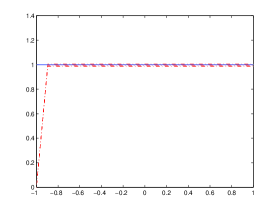
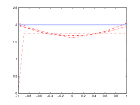
$-$ : true function	$-$ : true function
$-.$ : estimator	$-.$ : estimator
$n=10^{5}$, $\Delta=10^{-3}$	$n=10^{5}$, $\Delta=0.1$

Figure 2: Model 2

$$dX_{t}=-2X_{t}dt+\frac{X_{t^{-}}^{2}+3}{X_{t^{-}}^{2}+1}dW_{t}+dL_{t},\quad\textrm{Laplace jumps}$$

Estimation of $\sigma^{2}$	Estimation of $\sigma^{2}+\xi^{2}$
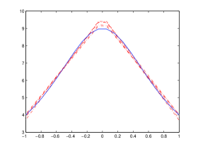
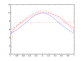
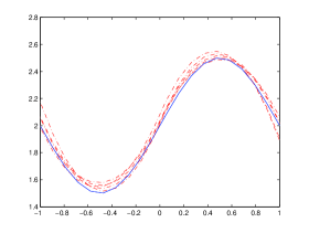
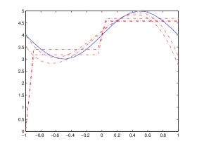
$-$ : true function	$-$: true function
$-.$ : estimator	$-.$ : estimator
$n=10^{5}$, $\Delta=10^{-3}$	$n=10^{5}$, $\Delta=10^{-2}$

Figure 3: Model 3

$$dX_{t}=(-2X_{t}+\sin(3X_{t}))dt+\sqrt{2+0.5\sin(\pi X_{t^{-}})}(dW_{t}+dL_{t}),\quad\textrm{Normal jumps}$$

Estimation of $\sigma^{2}$	Estimation of $\sigma^{2}+\xi^{2}$
$-$ : true function	$-$ : true function
$-.$ : estimator	$-.$ : estimator
$n=10^{5}$, $\Delta=10^{-3}$	$n=10^{5}$, $\Delta=10^{-2}$

Figure 4: Model 4

$$n(z)=\sum_{k=1}^{\infty}2^{k+1}(\delta_{1/2^{k}}+\delta_{-1/2^{k}}),\quad b(x)=-2x\quad\textrm{and}\quad\sigma(x)=\xi(x)=1.$$

Estimation of $\sigma^{2}$	Estimation of $\sigma^{2}+\xi^{2}$
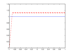
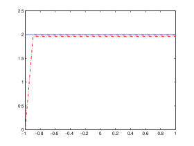
$-$ : true function	$-$ : true function
_. : estimator	_. : estimator
$n=10^{5}$, $\Delta=10^{-4}$	$n=10^{5}$, $\Delta=10^{-2}$

Table 1: Model 1

$$dX_{t}=-2X_{t}dt+dW_{t}+dL_{t},\quad\textrm{binomial jumps}$$

		Estimation of $\sigma^{2}+\xi^{2}$					Estimation of $\sigma^{2}$
$\Delta$	$n$	risk	oracle	$m_{est}$	$r_{est}$	$t_{e}$	risk	oracle	$m_{est}$	$r_{est}$	$t_{e}$
$10^{-1}$	$10^{3}$	0.075	1.00	0.00	0.92	0.78	0.93	1.56	1.92	0.92	0.78
$10^{-1}$	$10^{4}$	0.061	1.03	0.02	1.30	3.61	0.63	1.12	3.44	1.30	3.61
$10^{-1}$	$10^{5}$	0.066	1.14	0.16	1.46	36	0.59	1.03	3.46	1.46	36
$10^{-2}$	$10^{3}$	0.15	1.00	0.00	0.00	0.22	0.0026	1.71	0.02	0.00	0.22
$10^{-2}$	$10^{4}$	0.015	1.00	0.00	0.00	3.60	0.0004	3.27	0.02	0.00	3.60
$10^{-2}$	$10^{5}$	0.0021	1.00	0.00	0.52	36	0.00048	4.70	0.12	0.52	36
$10^{-3}$	$10^{3}$	4.18	1.21	0.02	0.00	0.13	0.0020	1.00	0.00	0.00	0.13
$10^{-3}$	$10^{4}$	0.12	1.00	0.00	0.00	0.58	0.0002	1.00	0.00	0.00	0.58
$10^{-3}$	$10^{5}$	0.013	1.00	0.00	0.02	36	0.000022	1.57	0.00	0.02	36

Table 2: Model 2

$$dX_{t}=-2X_{t}dt+\frac{X_{t^{-}}^{2}+3}{X_{t^{-}}^{2}+1}dW_{t}+dL_{t},\quad\textrm{Laplace jumps}$$

		Estimation of $\sigma^{2}+\xi^{2}$					Estimation of $\sigma^{2}$
$\Delta$	$n$	risk	oracle	$m_{est}$	$r_{est}$	$t_{e}$	risk	oracle	$m_{est}$	$r_{est}$	$t_{e}$
$10^{-1}$	$10^{3}$	3.53	2.46	0.00	0.02	0.78	3.02	3.04	0.00	0.02	0.77
$10^{-1}$	$10^{4}$	3.07	2.05	0.00	0.42	2.54	2.23	1.68	0.14	0.42	2.54
$10^{-1}$	$10^{5}$	1.51	1.01	0.52	1.58	20.4	1.26	1.01	0.46	1.58	20.4
$10^{-2}$	$10^{3}$	152	5.00	0.20	0.08	0.23	2.81	10.5	0.02	0.08	0.23
$10^{-2}$	$10^{4}$	3.37	5.69	0.00	1.28	2.56	0.28	1.25	0.72	1.28	2.53
$10^{-2}$	$10^{5}$	1.36	1.39	0.54	1.08	20.3	0.22	1.05	1.00	1.08	20.3
$10^{-3}$	$10^{3}$	1600	2.87	0.02	0.20	0.14	2.34	10.2	0.16	0.20	0.14
$10^{-3}$	$10^{4}$	85	3.60	0.10	1.16	0.56	0.087	1.47	0.84	1.16	0.56
$10^{-3}$	$10^{5}$	4.90	6.58	0.00	1.00	20.3	0.023	3.23	1.00	1.00	20.3

Table 3: Model 3

$$dX_{t}=(-2X_{t}+\sin(3X_{t}))dt+\sqrt{2+0.5\sin(\pi X_{t^{-}})}(dW_{t}+dL_{t}),\quad\textrm{Normal jumps}$$

		Estimation of $\sigma^{2}+\xi^{2}$					Estimation of $\sigma^{2}$
$\Delta$	$n$	risk	oracle	$m_{est}$	$r_{est}$	$t_{e}$	risk	oracle	$m_{est}$	$r_{est}$	$t_{e}$
$10^{-1}$	$10^{3}$	1.00	1.86	0.02	1.10	0.81	15.4	7.15	4.52	1.10	0.80
$10^{-1}$	$10^{4}$	0.56	1.27	0.48	1.20	3.43	3.43	1.71	5.72	1.20	3.39
$10^{-1}$	$10^{5}$	0.43	1.03	0.90	1.00	31.3	2.09	1.08	6.24	1.00	31.2
$10^{-2}$	$10^{3}$	24.4	28.5	0.32	0.62	0.24	2.49	8.59	1.66	0.62	0.24
$10^{-2}$	$10^{4}$	0.78	2.57	0.12	1.30	3.41	1.46	4.34	4.88	1.30	3.38
$10^{-2}$	$10^{5}$	0.12	3.30	0.82	1.10	31.1	0.75	1.54	6.98	1.10	31.0
$10^{-3}$	$10^{3}$	82.3	3.57	0.08	0.08	0.14	0.090	5.43	0.12	0.08	0.14
$10^{-3}$	$10^{4}$	13.1	2.51	0.18	1.14	0.60	0.019	4.61	0.80	1.14	0.61
$10^{-3}$	$10^{5}$	0.98	2.63	0.26	2.18	31	0.0026	1.16	0.82	2.18	30.8

Table 4: Model 4

$$n(z)=\sum_{k=1}^{\infty}2^{k+1}(\delta_{1/2^{k}}+\delta_{-1/2^{k}}),\quad b(x)=-2x\quad\textrm{and}\quad\sigma(x)=\xi(x)=1.$$

		Estimation of $\sigma^{2}+\xi^{2}$					Estimation of $\sigma^{2}$
$\Delta$	$n$	risk	oracle	$m_{est}$	$r_{est}$	$t_{e}$	risk	oracle	$m_{est}$	$r_{est}$	$t_{e}$
$10^{-1}$	$10^{3}$	0.074	1.00	0.00	0.14	0.86	0.56	1.02	0.06	0.14	0.89
$10^{-1}$	$10^{4}$	0.075	1.01	0.02	1.28	4.04	0.54	1.02	0.30	1.28	4.01
$10^{-1}$	$10^{5}$	0.080	1.02	0.12	1.98	37.4	0.55	1.02	0.12	1.98	37.3
$10^{-2}$	$10^{3}$	0.039	1.00	0.00	0.42	0.25	0.96	1.19	0.70	0.42	0.25
$10^{-2}$	$10^{4}$	0.0040	1.00	0.00	0.62	4.57	0.86	1.01	0.72	0.62	4.58
$10^{-2}$	$10^{5}$	0.0012	1.00	0.00	0.58	38.3	0.91	1.00	1.24	0.58	38.1
$10^{-3}$	$10^{3}$	1.22	1258	0.04	1.02	0.14	0.071	1.07	0.04	0.02	0.15
$10^{-3}$	$10^{4}$	0.012	1.00	0.00	0.10	0.87	0.094	1.01	0.02	0.10	0.87
$10^{-3}$	$10^{5}$	0.0015	1.00	0.00	0.36	38.5	0.15	1.00	0.22	0.36	38.5
$10^{-4}$	$10^{4}$	0.24	1.00	0.00	0.02	0.39	0.013	1.04	0.02	0.02	0.39
$10^{-4}$	$10^{5}$	0.021	1.00	0.00	0.04	6.31	0.014	1.00	0.00	0.04	6.26

6 Proofs

6.1 Proof of Theorem 4

By Lemma 2, $\mathbb{E}\left(A_{k\Delta}^{2}\right)\lesssim\Delta$. It remains to bound $\mathbb{E}\left(\sup_{t\in\mathscr{B}_{m}}\nu_{n}^{2}(t)\right)$. Let $\left(\varphi_{\lambda}\right)_{1\leq\lambda\leq D_{m}}$ be an orthonormal (for the $\|.\|_{\pi}$ norm) basis of $S_{m}$. Any function $t\in\mathscr{B}_{m}$ can be written $t=\sum_{\lambda=1}^{D_{m}}a_{\lambda}\varphi_{\lambda}$ with $\sum_{\lambda=1}^{D_{m}}a_{\lambda}^{2}\leq 1$. By Cauchy-Schwarz,

$$\sup_{t\in\mathscr{B}_{m}}\nu_{n}^{2}(t)=\sup_{\sum_{\lambda=1}^{D_{m}}a_{\lambda}^{2}\leq 1}\left(\sum_{\lambda=1}^{D_{m}}a_{\lambda}^{2}\right)\left(\sum_{\lambda=1}^{D_{m}}\nu_{n}^{2}\left(\varphi_{\lambda}\right)\right)\leq\sum_{\lambda=1}^{D_{m}}\nu_{n}^{2}(\varphi_{\lambda}).$$

According to Lemma 2, $\mathbb{E}\left(B_{k\Delta}+E_{k\Delta}\left|\mathscr{F}_{k\Delta}\right.\right)=0$, and

$$\mathbb{E}\left(\nu_{n}^{2}(\varphi_{\lambda})\right) =\mathbb{E}\left[\left(\frac{1}{n}\sum_{k=1}^{n}\left(B_{k\Delta}+E_{k\Delta}\right)\varphi_{\lambda}(X_{k\Delta})\right)^{2}\right]$$

$$\leq\frac{2}{n^{2}}\sum_{k=1}^{n}\mathbb{E}\left[\varphi_{\lambda}^{2}(X_{k\Delta})\mathbb{E}\left(B_{k\Delta}^{2}+E_{k\Delta}^{2}\left|\mathscr{F}_{k\Delta}\right.\right)\right]$$

$$\lesssim\frac{\xi_{0}^{4}}{n\Delta}+\frac{\sigma_{0}^{4}+\sigma_{0}^{2}\xi_{0}^{2}}{n}.$$

Then

$$\mathbb{E}\left(\sup_{t\in\mathscr{B}_{m}}\nu_{n}^{2}(t)\right)\lesssim\left(\frac{\xi_{0}^{4}}{\Delta}+\sigma_{0}^{4}+\sigma_{0}^{2}\xi_{0}^{2}\right)\frac{D_{m}}{n}$$ (2)

It remains to bound the risk on $\Omega_{n}^{c}$.  By Lemma 3, $\mathbb{P}\left(\Omega_{n}^{c}\right)\leq 1/n^{8}$. The function $\hat{g}_{m}$ is the orthogonal projection (for the $\|.\|_{n}$ norm) of $(T_{\Delta},\ldots,T_{n\Delta})$ on the vectorial subspace $\left\{(t(X_{\Delta}),\ldots,t(X_{n\Delta}))\>,t\in S_{m}\right\}$. Let us denote by $\Pi_{m}$ the orthogonal projection on this subspace. As $T_{k\Delta}=g(X_{k\Delta})+A_{k\Delta}+B_{k\Delta}+E_{k\Delta}$, we obtain:

$$\|\hat{g}_{m}-g_{A}\|_{n}^{2} =\|\Pi_{m}T-g_{A}\|_{n}^{2}=\|\Pi_{m}g_{A}-g_{A}\|_{n}^{2}+\|\Pi_{m}A+\Pi_{m}B+\Pi_{m}E\|_{n}^{2}$$

$$\leq\|g_{A}\|_{n}^{2}+\|A+B+E\|_{n}^{2}$$

By stationarity and Cauchy-Schwarz:

$$\mathbb{E}\left(\|\hat{g}_{m}-g_{A}\|_{n}^{2}\mathbbmss{1}_{\Omega_{n}^{c}}\right) \lesssim\mathbb{E}\left(\|g_{A}\|_{n}^{2}\mathbbmss{1}_{\Omega_{n}^{c}}\right)+\mathbb{E}\left[\left(\frac{1}{n}\sum_{k=1}^{n}A_{k\Delta}^{2}+B_{k\Delta}^{2}+E_{k\Delta}^{2}\right)\mathbbmss{1}_{\Omega_{n}^{c}}\right]$$

$$\lesssim\left[\left(\mathbb{E}\left[\|g_{A}\|_{n}^{4}\right]+\mathbb{E}\left[A_{k\Delta}^{4}+B_{k\Delta}^{4}+E_{k\Delta}^{4}\right]\right)\mathbb{P}\left(\Omega_{n}^{c}\right)\right]^{1/2}.$$

By Lemmas 2 and 3, we obtain:

$$\mathbb{E}\left(\|\hat{g}_{m}-g_{A}\|_{n}^{2}\mathbbmss{1}_{\Omega_{n}^{c}}\right)\lesssim\frac{1}{\Delta^{3/2}n^{4}}\leq\frac{1}{n}.$$

6.2 Proof of Theorem 5

First, we apply the Berbee’s coupling lemma to the random vectors $(B_{k\Delta}+E_{k\Delta},X_{k\Delta})$ which are exponentially $\beta$-mixing. According to Berbee’s coupling lemma, we can construct independent variables

$$U_{k,a}^{*}=\frac{1}{q_{n}}\sum_{l=1}^{q_{n}}\left(B+E\right)_{(2(k-1)+a)q_{n}+l)\Delta}^{*}t(X_{(2(k-1+a)q_{n}+l)\Delta}^{*})$$

such that for $a\in\left\{0,1\right\}$, the random variables $(U_{k,a}^{*})_{0\leq k\leq p_{n}}$ are independent and have same law as

$$U_{k,a}=\frac{1}{q_{n}}\sum_{l=1}^{q_{n}}\left(B+E\right)_{(2(k-1)+a)q_{n}+l)\Delta}t(X_{(2(k-1+a)q_{n}+l)\Delta}).$$

Let us set

$$\Omega^{*}=\left\{\omega,\>\forall a,\>\forall k,\>U_{k,a}=U_{k,a}^{*}\right\},$$

$$\Omega_{B,\alpha}=\left\{\omega,\>\forall(a,k),\>\left|U_{k,a}^{*}\right|\leq c\ln^{2}(n)D^{1/2}\Delta^{-\alpha}\right\}$$

and

$$\mathscr{O}=\Omega_{n}\cap\Omega_{B,\alpha}\cap\Omega^{*}$$

with $D=D_{m}+D_{m^{\prime}}$. By Berbee’s coupling lemma,

$$\mathbb{P}\left(\Omega^{*c}\right)\lesssim n\Delta/n^{8}.$$

The following lemma is proved later.

Lemma 12.

For any $\alpha>0$, there exists a constant $c$ such that

$$\mathbb{P}\left(\Omega_{B,\alpha}^{c}\right)\lesssim\frac{1}{n^{5}}.$$

Then

$$\mathbb{P}\left(\mathscr{O}^{c}\right)\leq\mathbb{P}(\Omega_{B,\alpha}^{c})+\mathbb{P}(\Omega^{*c})+\mathbb{P}(\Omega_{n}^{c})\lesssim\frac{1}{n^{5}}+\frac{n\Delta}{n^{8}}+\frac{1}{n^{8}}\lesssim\frac{1}{n^{5}}.$$

We can bound $\mathbb{E}\left(\|\hat{g}_{\hat{m}}-g\|_{n}^{2}\mathbbmss{1}_{\mathscr{O}^{c}}\right)$ in the same way as we bound the risk of the non-adaptive estimator on $\Omega_{n}^{c}$:

$$\mathbb{E}\left(\|\hat{g}_{\hat{m}}-g_{A}\|_{n}^{2}\mathbbmss{1}_{\mathscr{O}^{c}}\right)\lesssim\frac{1}{\Delta^{3/2}n^{5/2}}\lesssim\frac{1}{n}.$$

It remains to bound the risk on $\mathscr{O}$. Let us set, for $a\in\left\{0,1\right\}$,

$$\nu_{n,a}^{*}(t)=\frac{1}{p_{n}}\sum_{k=1}^{p_{n}}U_{k,a}^{*}\mathbbmss{1}_{\mathscr{O}}-\mathbb{E}\left(U_{k,a}^{*}\mathbbmss{1}_{\mathscr{O}}\right)$$

and $\nu_{n}^{*}(t)=\nu_{n,0}^{*}(t)+\nu_{n,1}^{*}(t)$. We have:

$$\|\hat{g}_{\hat{m}}-g\|_{n}^{2}\mathbbmss{1}_{\mathscr{O}}\lesssim\frac{1}{n}\sum_{k=1}^{n}A_{k\Delta}^{2}+\left(\mathbb{E}\left[\left(B_{k\Delta}^{*}+E_{k\Delta}^{*}\right)\mathbbmss{1}_{\mathscr{O}}\right]\right)^{2}+\sup_{t\in\mathscr{B}_{m,\hat{m}}}\left(\nu_{n}^{*}(t)\right)^{2}+2pen(m).$$

As the random variables $B_{k\Delta}^{*}$ and $E_{k\Delta}^{*}$ are centred,

$$R_{1}:=\mathbb{E}\left[\left(B_{k\Delta}^{*}+E_{k\Delta}^{*}\right)\mathbbmss{1}_{\mathscr{O}}\right]=-\mathbb{E}\left[\left(B_{k\Delta}^{*}+E_{k\Delta}^{*}\right)\mathbbmss{1}_{\mathscr{O}^{c}}\right]$$

then by Lemma 2,

$$\left|R_{1}\right|\lesssim\left(\mathbb{E}\left[\left(B_{k\Delta}^{*}+E_{k\Delta}^{*}\right)^{2}\right]\mathbb{P}\left(\mathscr{O}^{c}\right)\right)^{1/2}\leq n^{-5/2}\Delta^{-1/2}.$$

Then

$$\mathbb{E}\left(\|\hat{g}_{\hat{m}}-g_{A}\|_{n}^{2}\mathbbmss{1}_{\mathscr{O}}\right) \lesssim\|g_{m}-g\|_{L^{2}}^{2}+\Delta+\frac{1}{n}+2pen(m)$$

$$+12\mathbb{E}\left(\sum_{m^{\prime}\in\mathscr{M}_{n}}\left[\left(\sup_{t\in\mathscr{B}_{m,m^{\prime}}}\left(\nu_{n}^{*}(t)\right)^{2}-p(m,m^{\prime})\right)\mathbbmss{1}_{\mathscr{O}}\right]_{+}\right)$$

The functions $\nu_{n,a}^{*}(t)$ satisfy the assumptions of Talagrand’s inequality with $M=c\ln^{2}(n)D^{1/2}\Delta^{-\alpha}$, $V=\frac{1}{q_{n}\Delta}$, and $H^{2}=c^{\prime}D/(n\Delta)$. Then

$$R_{2} :=\mathbb{E}\left(\left[\sup_{t\in\mathscr{B}_{m,m^{\prime}}}\left(\nu_{n}^{*}(t)\right)^{2}-12p(m,m^{\prime})\right]_{+}\right)$$

$$\lesssim\frac{1}{n\Delta}\exp\left(-c^{\prime}\frac{p_{n}q_{n}\Delta}{n\Delta}D\right)+\frac{c^{2}\ln^{4}(n)D\Delta^{-2\alpha}}{p_{n}^{2}}\exp\left(-\frac{c^{\prime}}{c}\frac{p_{n}D^{1/2}}{\sqrt{n\Delta}\Delta^{-\alpha}D^{1/2}\ln^{2}(n)}\right)$$

$$\lesssim\frac{1}{n\Delta}\exp\left(-cD\right)+\frac{\ln^{6}(n)}{n^{2}\Delta^{2+2\alpha}}D\exp\left(-c^{\prime}\frac{\sqrt{n\Delta^{1+2\alpha}}}{\ln^{3}(n)}\right).$$

Consequently, as $\alpha$ is as small as we want:

$$\mathbb{E}\left(\left[\sup_{t\in\mathscr{B}_{m,\hat{m}}}\nu_{n}^{2}(t)-pen(m)\right]_{+}\right)\lesssim\frac{1}{n\Delta}\sum_{m^{\prime}}e^{-cD_{m,m^{\prime}}}\lesssim\frac{1}{n\Delta}.$$

6.3 Proof of Lemma 12

We have that

$$U_{1,0}^{*}=\frac{1}{q_{n}}\sum_{j=1}^{q_{n}}(B_{j\Delta}^{*}+E_{j\Delta}^{*})t(X_{j\Delta}^{*})\lesssim\frac{1}{q_{n}\Delta}\sum_{j=1}^{q_{n}}\left(J_{j\Delta}^{2}+Z_{j\Delta}^{2}\right)t(X_{j\Delta}).$$

We know that $\left|t(X_{j\Delta})\right|\leq\|t\|_{\infty}\lesssim D^{1/2}$. Moreover,

$$\mathbb{P}\left(\left|Z_{k\Delta}\right|\geq k\sigma_{0}\Delta^{1/2}\ln(n)\right) \leq n^{-k}\mathbb{E}\left[\exp\left(\frac{1}{\sigma_{0}\Delta^{1/2}}Z_{k\Delta}\right)\right]$$

$$\leq n^{-k}\mathbb{E}\left[\exp\left(\frac{1}{\sigma_{0}^{2}\Delta}\int_{k\Delta}^{(k+1)\Delta}\sigma^{2}(X_{s})ds\right)\right]$$

$$\leq n^{-k}.$$ (3)

Then

$$\mathbb{P}\left(\left|Z_{k\Delta}\right|\geq 6\sigma_{0}^{2}\Delta\ln(n)\right)\lesssim n^{-6}.$$ (4)

and then

$$\sum_{k=1}^{p_{n}}\mathbb{P}\left(\frac{1}{q_{n}}\sum_{j=1}^{q_{n}}Z_{j\Delta}^{2}\geq 36\sigma_{0}^{4}\Delta\ln^{2}(n)\right)\lesssim n^{-5}.$$

Bound of $\mathbb{P}\left(\left|J_{k\Delta}^{(1)}\right|\geq 12\xi_{0}\Delta^{1/2}\ln(n)\right)$.

The terms $J_{k\Delta}^{(1)}$ are small and can be bounded in the same way as the Brownian terms $Z_{k\Delta}$. As $\nu$ is symmetric:

$$\mathbb{P}\left(\left|J_{k\Delta}^{(1)}\right|\geq 12\xi_{0}\Delta^{1/2}\ln(n)\right) \leq 2\mathbb{P}\left(\exp\left(aJ_{k\Delta}^{(1)}\right)\geq\exp\left(12a\xi_{0}\Delta^{1/2}\ln(n)\right)\right)$$

$$\leq 2\exp\left(-12a\xi_{0}\Delta^{1/2}\ln(n)\right)\mathbb{E}\left(\exp\left(aJ_{k\Delta}^{(1)}\right)\right).$$

According to Corollary 5.2.2 of Applebaum (2004),

$$\mathbb{E}\left(\exp\left(aJ_{k\Delta}^{(1)}\right)\right)=\mathbb{E}\left(\exp\left(\int_{k\Delta}^{(k+1)\Delta}\int_{-\Delta^{1/2}}^{\Delta^{1/2}}\left(e^{a\xi(X_{s-})z}-1-a\xi(X_{s^{-}})z\right)\nu(dz)ds\right)\right).$$

Then for any $a\leq 1/(2\xi_{0}\Delta^{1/2})$,

$$\mathbb{E}\left(\exp\left(aJ_{k\Delta}^{(1)}\right)\right) \leq\mathbb{E}\left(\exp\left(\int_{k\Delta}^{(k+1)\Delta}\int_{-\Delta^{1/2}}^{\Delta^{1/2}}a^{2}z^{2}\xi^{2}(X_{s^{-}})\nu(dz)\right)\right)$$

$$\leq\mathbb{E}\left(\exp\left(\xi_{0}^{2}a^{2}\Delta^{\text{2-$\beta$/2}}\right)\right).$$

Let us then set $a=1/(2\xi_{0}\Delta^{1/2})$, we obtain:

$$\mathbb{P}\left(\left|J_{k\Delta}^{(1)}\right|\geq 12\xi_{0}\Delta^{1/2}\ln(n)\right)\lesssim\exp\left(-6\ln(n)\right)\leq n^{-6}.$$ (5)

Bound for the jumps greater than $\Delta^{1/2}$.

The probability that

$$J_{k\Delta}^{(2)}+J_{k\Delta}^{(3)}\geq\Delta^{1/2}\ln(n)$$

is not small enough. We have to bound both the number of jumps of the time interval $[k\Delta,(k+1)\Delta[$ and the size of the jumps. Let us first consider the jumps greater than 1:

$$J_{k\Delta}^{(0)}=\int_{k\Delta}^{(k+1)\Delta}\xi(X_{s^{-}})\int_{\left|z\right|\geq 1}\mu(dz,ds).$$

The probability of having a very high jump is quite small: by Assumption A4,

$$\nu\left(\left[-\frac{8\ln(n)}{\lambda},\frac{8\ln(n)}{\lambda}\right]^{c}\right)\lesssim n^{-8}.$$ (6)

The probability of having more than $C=8\eta/(1-\beta/2)$ (see Assumption A4) jumps greater than $1$ on a time interval $\Delta$ is very low:

$$Q_{1} :=\mathbb{P}\left(\mu\left(\left[k\Delta,(k+1)\Delta\right[,\left[-1,1\right]^{c}\right)\geq C\right)$$

$$\leq\mathbb{P}\left(\mu\left(\left[k\Delta,(k+1)\Delta\right[,\left[-\Delta^{1/2},\Delta^{1/2}\right]^{c}\right)\geq C\right)$$

$$\leq\left(\Delta\int_{\left|z\right|>\Delta^{1/2}}\nu(dz)\right)^{C}\lesssim\left(\Delta^{1-\beta/2}\right)^{C}=\Delta^{8\eta}\lesssim n^{-8}.$$ (7)

By (6) and (7),

$$\mathbb{P}\left(|J_{k\Delta}^{(0)}|\geq\frac{8C\ln(n)}{\lambda}\right)\lesssim n^{-8}.$$

Let us set $v_{1}=\nu(]-1,1[^{c})\vee 1$. We have that

$$Q_{2} :=\mathbb{P}\left(\frac{1}{q_{n}}\sum_{k=1}^{q_{n}}\left|J_{k\Delta}^{(0)}\right|^{2}\geq\frac{8^{2}C^{2}}{\lambda^{2}}v_{1}\Delta\ln^{2}(n)\right)$$

$$\lesssim q_{n}\mathbb{P}\left(|J_{k\Delta}^{(0)}|\geq\frac{8C\ln(n)}{\lambda}\right)+\mathbb{P}\left[\mu\left([0,q_{n}\Delta[,[-1,1]^{c}\right)\geq v_{1}\Delta q_{n}\right]$$

$$\lesssim\frac{q_{n}}{n^{8}}+\sum_{j\geq v_{1}\Delta q_{n}}^{+\infty}\frac{\left(q_{n}\Delta v_{1}\right)^{j}}{j!}e^{-q_{n}\Delta v_{1}}$$

$$\lesssim\frac{q_{n}}{n^{8}}+\sum_{j\geq 8v_{1}\ln(n)}^{+\infty}\left(\frac{8\ln(n)v_{1}e}{j}\right)^{j}\sqrt{j}e^{-8\ln(n)v_{1}}$$

$$\lesssim\frac{q_{n}}{n^{8}}+\frac{1}{n^{8}}.$$ (8)

Let us now set $\alpha_{0}=0$, $\alpha_{j}=\frac{2\alpha_{j-1}+\alpha}{\beta}\wedge\frac{1}{2}$ and

$$J_{k\Delta}^{(\alpha_{j})}=\int_{k\Delta}^{(k+1)\Delta}\int_{[-\Delta^{\alpha_{j-1}},-\Delta^{\alpha_{j}}]\cup[\Delta^{\alpha_{j}},\Delta^{\alpha_{j-1}}]}\xi(X_{s^{-}})dL_{s}.$$

By (7),

$$\mathbb{P}\left(\left|J_{k\Delta}^{(\alpha_{j})}\right|\geq C\Delta^{\alpha_{j-1}}\right)\lesssim\frac{1}{n^{8}}.$$

We have that $\nu\left(\left[-\Delta^{-\alpha_{j-1}},-\Delta^{\alpha_{j}}\right]\cup\left[\Delta^{\alpha_{j}},\Delta^{\alpha_{j-1}}\right]\right)\lesssim\Delta^{-\alpha_{j}\beta}$. Let us set $v_{2}=\Delta^{\beta\alpha_{j}}\left(\nu(\left[-\Delta^{-\alpha_{j-1}},-\Delta^{\alpha_{j}}\right]\cup\left[\Delta^{\alpha_{j}},\Delta^{\alpha_{j-1}}\right])\vee 1\right).$ Then

$$Q_{3} :=\mathbb{P}\left(\frac{1}{q_{n}}\sum_{k=1}^{q_{n}}\left|J_{k\Delta}^{\left(\alpha_{j}\right)}\right|^{2}\geq C^{2}\Delta^{1-\alpha}\right)$$

$$\leq\mathbb{P}\left[\mu\left(\left[0,q_{n}\Delta\right[,\left[-\Delta^{-\alpha_{j-1}},-\Delta^{\alpha_{j}}\right]\cup\left[\Delta^{\alpha_{j}},\Delta^{\alpha_{j-1}}\right]\right)\geq q_{n}\Delta^{1-2\alpha_{j-1}-\alpha}\right]$$

$$+q_{n}\mathbb{P}\left(\left|J_{k\Delta}^{(\alpha_{j})}\right|\geq C\Delta^{\alpha_{j-1}}\right)$$

$$\lesssim\frac{q_{n}}{n^{8}}+\sum_{i=q_{n}\Delta^{1-2\alpha_{j-1}-\alpha}}^{\infty}\frac{\left(q_{n}\Delta v_{2}\Delta^{-\beta\alpha_{j}}\right)^{i}}{i!}e^{-q_{n}\Delta v_{2}\Delta^{-\beta\alpha_{j}}}$$

$$\lesssim n^{-8}.$$ (9)

Then, by (4), (5), (8) and (9), we obtain:

$$\mathbb{P}\left(\Omega_{B,\alpha}^{c}\right)\lesssim\frac{p_{n}q_{n}}{n^{6}}+\frac{p_{n}q_{n}}{n^{8}}\lesssim n^{-5}.$$

6.4 Proof of Lemma 6

Bound of $\mathbb{P}\left(\Omega_{X,k}^{c}\right)$.

We have that $X_{(k+1)\Delta}=X_{k\Delta}+\int_{k\Delta}^{(k+1)\Delta}b(X_{s})ds+Z_{k\Delta}+J_{k\Delta}$. Then

$$\mathbb{P}\left(\Omega_{X,k}^{c}\right) \leq\mathbb{P}\left(\left|\int_{k\Delta}^{(k+1)\Delta}b(X_{s})ds\right|\geq\Delta^{1/2}\right)+\mathbb{P}\left(\left|Z_{k\Delta}\right|\geq\sigma_{0}\Delta^{1/2}\ln(n)\right)$$

$$+\mathbb{P}\left(\left|J_{k\Delta}\right|\geq\xi_{0}\Delta^{1/2}\ln(n)\right).$$

By Markov’s inequalities, for any $k\leq 4$:

$$\mathbb{P}\left(\left|\int_{k\Delta}^{(k+1)\Delta}b(X_{s})ds\right|\geq\Delta^{1/2}\right)\lesssim\Delta^{-k}\mathbb{E}\left[\left(\int_{k\Delta}^{(k+1)\Delta}b(X_{s})ds\right)^{2k}\right]\lesssim\Delta^{k}$$ (10)

and by (3), $\mathbb{P}\left(\left|Z_{k\Delta}\right|\geq k\sigma_{0\mbox{}}\Delta^{1/2}\ln(n)\right)\lesssim n^{-k}.$ Moreover,

$$\mathbb{P}\left(\left|J_{k\Delta}^{(2)}+J_{k\Delta}^{(3)}\right|>0\right) \leq\Delta\int_{[-\Delta^{1/2},\Delta^{1/2}]^{c}}\nu(dz)\leq\Delta\Delta^{-\beta/2}\int_{[-\Delta^{1/2},\Delta^{1/2}]^{c}}z^{\beta}\nu(dz)$$

$$\lesssim\Delta^{1-\beta/2}$$ (11)

and by Markov’s inequality:

$$\mathbb{P}\left(\left|J_{k\Delta}^{(1)}\right|>\xi_{0}\Delta^{1/2}\right) \leq\frac{1}{\xi_{0}^{2}\Delta}\mathbb{E}\left[\left(J_{k\Delta}^{(1)}\right)^{2}\right]$$

$$\leq\frac{1}{\xi_{0}^{2}\Delta}\Delta\xi_{0}^{2}\int_{-\Delta^{1/2}}^{\Delta^{1/2}}z^{2}\nu(dz)\lesssim\Delta^{1-\beta/2}\int_{-\Delta^{1/2}}^{\Delta^{1/2}}z^{\beta}\nu(dz)$$

$$\lesssim\Delta^{1-\beta/2}.$$ (12)

Bound of $\mathbb{P}\left(\Omega_{N,k}^{c}\right)$.

We have that

$$\mathbb{P}\left(N_{k}\geq 1\right)=\int_{k\Delta}^{(k+1)\Delta}\int_{|z|\geq\Delta^{1/4}}\nu(dz)\leq\Delta^{1-\beta/4}\int_{|z|\geq\Delta^{1/4}}z^{\beta}\nu(dz)\lesssim\Delta^{1-\beta/4}.$$

Then by (11) and (12), we obtain:

$$\mathbb{P}\left(\Omega_{N,k}^{c}\right) \leq\mathbb{P}\left(N_{k}\geq 1\right)+\mathbb{P}\left(|J_{k\Delta}^{(2)}+J_{k\Delta}^{(3)}|>0\right)+\mathbb{P}\left(\left|\int_{k\Delta}^{(k+1)\Delta}dL_{s}^{(1)}\right|\geq\ln(n)\Delta^{1/2}\right)$$

$$\lesssim\Delta^{1-\beta/2}.$$

Bound of $\mathbb{P}\left(\Omega_{X,k}\cap\Omega_{N,k}^{c}\right)$.

We have that

$$\mathbb{P}\left(\Omega_{X,k}\cap\left\{N_{k}\geq 1\right\}\right)\leq\mathbb{P}\left(N_{k}\geq 2\right)+\mathbb{P}\left(\Omega_{X,k}\cap\left\{N_{k}=1\right\}\right).$$

Now $\mathbb{P}\left(N_{k}\geq 2\right)\leq\left(\Delta^{1-\beta/4}\int_{|z|\geq\Delta^{1/4}}z^{\beta}\nu(dz)\right)^{2}\lesssim\Delta^{2-\beta/2}$. Moreover, if $N_{k}=1$, then $\left|J_{k\Delta}^{(3)}\right|\geq\xi_{1}\Delta^{1/4}$ and by conditional independence, we get:

$$S_{1} :=\mathbb{P}\left(\Omega_{X,k}\cap\left\{N_{k}=1\right\}\right)$$

$$\leq\mathbb{P}\left(N_{k}=1\right)\times\mathbb{P}\left(\left|\int_{k\Delta}^{(k+1)\Delta}b(X_{s})ds+Z_{k\Delta}+J_{k\Delta}^{(1)}+J_{k\Delta}^{(2)}\right|>\xi_{1}\Delta^{1/4}\right)$$

$$\leq\mathbb{P}\left(N_{k}=1\right)\left[\mathbb{P}\left(\left|\int_{k\Delta}^{(k+1)\Delta}b(X_{s})ds\right|\geq\frac{\xi_{1}\Delta^{1/4}}{3}\right)+\mathbb{P}\left(\left|Z_{k\Delta}\right|\geq\frac{\xi_{1}\Delta^{1/4}}{3}\right)\right]$$

$$+\mathbb{P}\left(N_{k}=1\right)\mathbb{P}\left(\left|J_{k\Delta}^{(1)}+J_{k\Delta}^{(2)}\right|\geq\frac{\xi_{1}\Delta^{1/4}}{3}\right).$$

By (10) and (3), $\mathbb{P}\left(\left|\int_{k\Delta}^{(k+1)\Delta}b(X_{s})ds\right|\geq c\Delta^{1/4}\right)\leq\Delta^{4}$ and, as $\ln(n)\ll\Delta^{-1/4}$, $\mathbb{P}\left(\left|Z_{k\Delta}\right|\geq c\Delta^{1/4}\right)\leq\mathbb{P}\left(\left|Z_{k\Delta}\right|\geq\ln(n)\Delta^{1/2}\right)\lesssim n^{-1}$. Moreover, by a Markov inequality, we obtain:

$$\mathbb{P}\left(\left|J_{k\Delta}^{(1)}+J_{k\Delta}^{(2)}\right|>c\Delta^{1/4}\right) \leq c^{-2}\Delta^{-1/2}\mathbb{E}\left[\left(J_{k\Delta}^{(1)}+J_{k\Delta}^{(2)}\right)^{2}\right]$$

$$\leq c^{-2}\Delta^{-1/2}\xi_{0}^{2}\Delta\int_{-\Delta^{1/4}}^{\Delta^{1/4}}z^{2}\nu(dz)$$

$$\lesssim\Delta^{1/2}\Delta^{1/2-\beta/4}.$$

As $\mathbb{P}\left(N_{k}=1\right)\lesssim\Delta^{1-\beta/4}$, we obtain:

$$\mathbb{P}\left(\Omega_{X,k}\cap\left\{N_{k}\geq 1\right\}\right)\lesssim\Delta^{2-\beta/2}.$$

Let us set $L_{s}^{(1)+(2)}=L_{s}^{(1)}+L_{s}^{(2)}$ and $J_{k\Delta}^{(1)+(2)}=J_{k\Delta}^{(1)}+J_{k\Delta}^{(2)}$. We consider

$$\mathscr{E}_{k}=\left\{\left|\int_{k\Delta}^{(k+1)\Delta}dL_{s}^{(1)+(2)}\right|\leq 4\frac{\xi_{0}+\sigma_{0}}{\xi_{1}}\Delta^{1/2}\ln(n)\right\}.$$

We have that

$$\mathscr{E}_{k}^{c} \subseteq\left\{\left|\xi(X_{k\Delta^{-}})\int_{k\Delta}^{(k+1)\Delta}dL_{s}^{(1)+(2)}\right|\geq 4(\xi_{0}+\sigma_{0})\Delta^{1/2}\ln(n)\right\}$$

$$\subseteq\left\{\left|J_{k\Delta}^{(1)+(2)}\right|\geq 2\left(\xi_{0}+\sigma_{0}\right)\Delta^{1/2}\ln(n)\right\}$$

$$\cup\left\{\left|\int_{k\Delta}^{(k+1)\Delta}\left(\xi(X_{s^{-}})-\xi(X_{k\Delta^{-}})\right)dL_{s}^{(1)+(2)}\right|\geq 2\left(\xi_{0}+\sigma_{0}\right)\Delta^{1/2}\ln(n)\right\}.$$

By (10) and (3),

$$S_{2} :=\mathbb{P}\left(\Omega_{X,k}\cap\left\{\left|J_{k\Delta}^{(1)+(2)}\right|\geq 2\left(\sigma_{0}+\xi_{0}\right)\Delta^{1/2}\ln(n)\right\}\cap N_{k}=0\right)$$

$$\lesssim\mathbb{P}\left(\left|\int_{k\Delta}^{(k+1)\Delta}b(X_{s})ds+Z_{k\Delta}\right|\geq\left(\sigma_{0}+\xi_{0}\right)\Delta^{1/2}\ln(n)\right)$$

$$\lesssim\Delta^{4}+n^{-1}.$$

By the Burkholder Davis Gundy inequality, we obtain that

$$\mathbb{E}\left(\sup_{s\leq(k+1)\Delta}\left(X_{s}-X_{k\Delta}\right)^{4}\mathbbmss{1}_{\Omega_{N,k}}\right)\lesssim\Delta^{2-\beta/4}.$$

Moreover,

$$S_{3} :=\mathbb{E}\left[\left(\int_{k\Delta}^{(k+1)\Delta}\left(\xi(X_{s^{-}})-\xi(X_{k\Delta^{-}})\right)dL_{s}^{(1)+(2)}\right)^{4}\right]$$

$$\lesssim\left(\int_{k\Delta}^{(k+1)\Delta}\Delta\int_{-\Delta^{1/4}}^{\Delta^{1/4}}z^{2}\nu(dz)\right)^{2}+\int_{k\Delta}^{(k+1)\Delta}\Delta^{2-\beta/4}\int_{-\Delta^{1/4}}^{\Delta^{1/4}}z^{4}\nu(dz)$$

$$\lesssim\Delta^{5-\beta/2}+\Delta^{4-\beta/2}\lesssim\Delta^{4-\beta/2}.$$ (13)

Then by a Markov’s inequality,

$$\mathbb{P}\left(\left|\int_{k\Delta}^{(k+1)\Delta}\left(\xi(X_{s^{-}})-\xi(X_{k\Delta^{-}})\right)dL_{s}^{(1)+(2)}\right|\geq\Delta^{1/2}\ln(n)\right)\lesssim\Delta^{2-\beta/2}$$

which ends the proof.

6.5 Proof of Lemma 7

From the Burkholder Davis Gundy inequality and Proposition 1, we derive easily the bounds for $\tilde{A}_{k\Delta}$ and $\tilde{B}_{k\Delta}$. It remains to bound $\mathbb{E}\left(\tilde{E}_{k\Delta}^{2}\left|\mathscr{F}_{k\Delta}\right.\right)$ and $\mathbb{E}\left(\tilde{E}_{k\Delta}^{4}\left|\mathscr{F}_{k\Delta}\right.\right)$. We first bound $\mathbb{E}\left(\left(J_{k\Delta}^{(1)+(2)}\right)^{4}\right)$. We have that

$$J_{k\Delta}^{(1)+(2)}=\int_{k\Delta}^{(k+1)\Delta}(\xi(X_{s^{-}})-\xi(X_{k\Delta^{-}}))dL_{s}^{(1)+(2)}+\xi(X_{k\Delta^{-}})\int_{k\Delta}^{(k+1)\Delta}dL_{s}^{(1)+(2)}.$$

By (13), $\mathbb{E}\left[\left(\int_{k\Delta}^{(k+1)\Delta}(\xi(X_{s^{-}})-\xi(X_{k\Delta^{-}}))dL_{s}^{(1)+(2)}\right)^{4}\right]\lesssim\Delta^{4-\beta/2}$. It remains to bound $\mathbb{E}\left[\left(\int_{k\Delta}^{(k+1)\Delta}dL_{s}^{(1)+(2)}\mathbbmss{1}_{\mathscr{E}_{k}}\right)^{4}\right].$ This is nearly Proposition 4.5 of Mai (2012). Let us introduce a nonnegative function $f$ $\mathscr{C}^{\infty}$ such that

$$\begin{cases}f(x)=x^{4}&\textrm{ if }|x|\leq 1\\ f(x)=0&\textrm{ if }|x|\geq 2.\end{cases}$$

Let us set $f^{a}(x)=a^{4}f(x/a)$. By stationarity, we have

$$\mathbb{E}\left[\left(\int_{k\Delta}^{(k+1)\Delta}dL_{s}^{(1)+(2)}\mathbbmss{1}_{\Omega_{N,k}}\right)^{4}\right]=\mathbb{E}\left[\left(L_{\Delta}^{(1)+(2)}\right)^{4}\mathbbmss{1}_{\Omega_{N,k}}\right]\leq\mathbb{E}\left(f^{\Delta^{1/2}\ln(n)}(L_{\Delta}^{(1)+(2)})\right).$$

The following result is needed.

Result 13.

[Fourier transform]

We denote by $\mathcal{F}h$ the Fourier transform of a function $h\in L^{1}(\mathbb{R})$:

$$\mathcal{F}h(x)=\int_{\mathbb{R}}f(u)e^{-ixu}du.$$

The Schwarz space is defined as

$$S\left(\mathbb{R}\right)=\left\{h\in\mathscr{C}^{\infty},\;\forall p,q\in\mathbb{N},\;\exists C_{p,q},\>\forall x\in\mathbb{R},\;|x^{p}h^{(q)}(x)|\leq C_{pq}\right\}.$$

Then we have the following properties:

1. For any $h_{1},h_{2}\in L^{2}(\mathbb{R})$, $(a_{1},a_{2})\in\mathbb{R}^{2}$, $\mathcal{F}(a_{1}h_{1}+a_{2}h_{2})=a_{1}\mathcal{F}h_{1}+a_{2}\mathcal{F}h_{2}$.

2. For any $h\in L^{2}(\mathbb{R})$, $\mathcal{F}h\in L^{2}(\mathbb{R})$ and $\forall x\in\mathbb{R},\;h(x)=\frac{1}{2\pi}\int_{\mathbb{R}}e^{itx}\mathcal{F}h(t)dt$.

3. For any $h\in L^{2}(\mathbb{R})$, $\mathcal{F}h(./a)(x)=|a|\mathcal{F}h(ax)$.

4. For any functions $h_{1},h_{2}\in L^{2}(\mathbb{R})$, the Parseval’s formula holds:

   $$\int_{\mathbb{R}}h_{1}(x)\overline{h_{2}(x)}dx=\frac{1}{2\pi}\int_{\mathbb{R}}\mathcal{F}h_{1}(u)\overline{\mathcal{F}h_{2}}(u)du.$$

   As $\mathcal{F}\delta_{y}(x)=e^{-ixy}$,

   $$h(0)=\int_{\mathbb{R}}h(y)\delta_{0}(y)dy=\frac{1}{2\pi}\int_{\mathbb{R}}\mathcal{F}h(u)du$$

5. For any $h$ in $S(\mathbb{R})$, $\mathcal{F}h\in S(\mathbb{R})$ and

   $$\mathcal{F}(h^{(q)})(x)=(ix)^{q}\mathcal{F}h(x).$$

By Result 13.4, we have that

$$\mathbb{E}\left(f^{a}(L_{t}^{(1)+(2)})\right) =\int_{\mathbb{R}}f^{a}(x)P_{L_{\Delta}^{(1)+(2)}}(dx)$$

$$=\frac{1}{2\pi}\int_{\mathbb{R}}\mathcal{F}f^{a}(u)\bar{\phi}_{\Delta}(u)du$$

where $\phi_{\Delta}$ is the characteristic function of the Lévy process $L_{\Delta}^{(1)+(2)}$:

$$\phi_{\Delta}(u)=\exp\left(\Delta\int_{-\Delta^{1/4}}^{\Delta^{1/4}}(e^{iux}-1-iux)\nu(dx)\right).$$

By a Taylor development in 0, we obtain that

$$\phi_{\Delta}(u)=1+\psi_{\Delta}(u)+R(\Delta,u)$$

with $\psi_{\Delta}(u)=\Delta\int_{-\Delta^{1/4}}^{\Delta^{1/4}}(e^{iux}-1-iux)\nu(dx)$. Then

$$\mathbb{E}\left(f^{a}(L_{t}^{(1)+(2)})\right) =\frac{1}{2\pi}\int_{\mathbb{R}}\mathcal{F}f^{a}(u)du+\frac{1}{2\pi}\int_{\mathbb{R}}\mathcal{F}f^{a}(u)\overline{\psi_{\Delta}(u)}du$$

$$+\frac{1}{2\pi}\int_{\mathbb{R}}\mathcal{F}f^{a}(u)\overline{R(\Delta,u)}du.$$

By Result 13.4, $\int_{\mathbb{R}}\mathcal{F}f^{a}(u)du=2\pi f^{a}(0)=0$ and consequently,

$$\int_{\mathbb{R}}\mathcal{F}f^{a}(u)\overline{\psi_{\Delta}(u)}du =\int_{\mathbb{R}}\mathcal{F}f^{a}(u)\Delta\int_{-\Delta^{1/4}}^{\Delta^{1/4}}(e^{-iux}-1+iux)du\nu(dx)$$

$$=\Delta\int_{-\Delta^{1/4}}^{\Delta^{1/4}}(2\pi)f^{a}(x)\nu(dx)-f^{a}(0)+\int_{\mathbb{R}}\mathcal{F}f^{a}(u)iuxdu\nu(dx).$$

By Result 13.5, as $f^{a}\in S(\mathbb{R})$, $\int_{\mathbb{R}}\mathcal{F}f^{a}(u)iudu=\int_{\mathbb{R}}\mathcal{F}((f^{a})^{\prime})(u)du=(f^{a})^{\prime}(0)=0$. Then

$$\int_{\mathbb{R}}\mathcal{F}f^{\Delta^{1/2}\ln(n)}(u)\overline{\psi_{\Delta}(u)}du =2\pi\Delta\int_{-\Delta^{1/4}}^{\Delta^{1/4}}f^{\Delta^{1/2}\ln(n)}(x)\nu(dx)$$

$$\lesssim\Delta\int_{-2\Delta^{1/2}\ln(n)}^{2\Delta^{1/2}\ln(n)}x^{4}\nu(dx)\lesssim\Delta\Delta^{2-\beta/2}\ln(n)^{4-\beta}.$$

It remains to bound $\mathbb{E}\left(\int_{\mathbb{R}}\mathcal{F}f^{a}(u)\overline{R(\Delta,u)}du\right)$. We have that

$$|R(\Delta,u)|=\left|e^{\psi_{\Delta}(u)}-\psi_{\Delta}(u)-1\right|\leq\left|\psi_{\Delta}^{2}(u)\right|.$$

According to Kappus (2012), $\left|\psi_{\Delta}(u)\right|\lesssim C\Delta|u|^{\beta}$. By Result 13.3, $\mathcal{F}f^{a}(u)=a^{5}\mathcal{F}f(au)$ and therefore

$$\left|\mathbb{E}\left(\int_{\mathbb{R}}\mathcal{F}f^{a}(u)\overline{R(\Delta,u)}du\right)\right| \lesssim\Delta^{2}\int_{\mathbb{R}}\left|\mathcal{F}f^{a}(u)\right||u|^{2\beta}du$$

$$\lesssim\Delta^{2}\int_{\mathbb{R}}a^{5}\left|\mathcal{F}f(au)\right||u|^{2\beta}du.$$

As $f^{a}\in S(\mathbb{R})$, $\mathcal{F}f^{a}\in S(\mathbb{R})$ and then for any $m>0$, $\exists C_{m}>0$, $|\mathcal{F}f(u)|\leq C_{m}|u|^{-m}$. Then, for any $m\in\mathbb{N}$:

$$\mathbb{E}\left(\int_{\mathbb{R}}\mathcal{F}f^{\Delta^{1/2}\ln(n)}(u)\overline{R(\Delta,u)}du\right)\lesssim\Delta^{2}\int_{\mathbb{R}}a^{5-m}|u|^{2\beta-m}\wedge a^{5}|u|^{2\beta}du.$$

We choose $m$ such that $2\beta+1<m\leq 3+\beta$. As $\beta<2$, $m$ always exists. Then $\int_{\mathbb{R}}|u|^{2\beta-m}\wedge|u|^{2\beta}<\infty$ and we get:

$$\mathbb{E}\left(\int_{\mathbb{R}}\mathcal{F}f^{\Delta^{1/2}\ln(n)}(u)\overline{R(\Delta,u)}du\right)\lesssim\Delta^{2}\left(\Delta^{1/2}\ln(n)\right)^{2-\beta}\lesssim\Delta^{3-\beta/2}\ln(n)^{2-\beta}$$

Then we obtain

$$\mathbb{E}\left[\left(J_{k\Delta}^{(1)+(2)}\right){}^{4}\mathbbmss{1}_{\mathscr{E}_{k}}\right] \lesssim\Delta^{3-\beta/2}\left(\ln(n)\right)^{4-\beta}.$$ (14)

Bound of $\mathbb{E}\left(\tilde{E}_{k\Delta}^{2}\mathbbmss{1}_{\Omega_{X,k}\cap\Omega_{N,k}}\right)$.

On $\Omega_{N,k}$,

$$\tilde{E}_{k\Delta}=\left(2b(X_{k\Delta})J_{k\Delta}^{(1)+(2)}+\frac{J_{k\Delta}^{(1)+(2)}}{\Delta}Z_{k\Delta}+\frac{\left(J_{k\Delta}^{(1)+(2)}\right)^{2}}{\Delta}\right)\mathbbmss{1}_{\mathscr{E}_{k}}.$$

Then by (14),

$$\mathbb{E}\left(\tilde{E}_{k\Delta}^{2}\mathbbmss{1}_{\Omega_{N,k}\cap\Omega_{X,k}}\right) \lesssim\frac{\mathbb{E}\left((J_{k\Delta}^{(1)+(2)})^{4}\mathbbmss{1}_{\mathscr{E}_{k}}\right)}{\Delta^{2}}+\mathbb{E}\left(Z_{k\Delta}^{4}\right)$$

$$\lesssim\Delta^{1-\beta/2}\ln(n)^{4-\beta}.$$

Bound of $\mathbb{E}\left(\tilde{E}_{k\Delta}^{2}\mathbbmss{1}_{\Omega_{X,k}\cap\Omega_{N,k}^{c}}\right)$.

We have that

$$S_{5} :=\mathbb{E}\left(\tilde{E}_{k\Delta}^{2}\mathbbmss{1}_{\Omega_{X,k}\cap\Omega_{N,k}^{c}}\right)$$

$$\leq\mathbb{E}\left(\tilde{E}_{k\Delta}^{2}\mathbbmss{1}_{\Omega_{X,k}\cap\Omega_{N,k}^{c}\cap\left\{\left|J_{k\Delta}\right|+\left|Z_{k\Delta}\right|\geq 9\sigma_{0}\ln(n)\Delta^{1/2}\right\}}\right)$$

$$+\mathbb{E}\left(\tilde{E}_{k\Delta}^{2}\mathbbmss{1}_{\Omega_{X,k}\cap\Omega_{N,k}^{c}\cap\left\{\left|J_{k\Delta}\right|+\left|Z_{k\Delta}\right|\leq 9\sigma_{0}\ln(n)\Delta^{1/2}\right\}}\right)$$

$$\lesssim\left(\mathbb{E}\left(\tilde{E}_{k\Delta}^{4}\right)\mathbb{P}\left(\Omega_{X,k}\cap\left\{\left|J_{k\Delta}\right|+\left|Z_{k\Delta}\right|\geq 9\sigma_{0}\ln(n)\Delta^{1/2}\right\}\right)\right)^{1/2}$$

$$+\ln^{2}(n)\mathbb{P}\left(\Omega_{X,k}\cap\Omega_{N,k}^{c}\right).$$

It remains to bound $\mathbb{P}\left(\Omega_{X,k}\cap\left\{\left|J_{k\Delta}\right|+\left|Z_{k\Delta}\right|\geq 9\sigma_{0}\ln(n)\Delta^{1/2}\right\}\right)$ . By inequality (3), $\mathbb{P}\left(\left|Z_{k\Delta}\right|\geq 4\sigma_{0}\ln(n)\Delta^{1/2}\right)\lesssim n^{-4}$ and

$$S_{6} :=\mathbb{P}\left(\left\{\left|J_{k\Delta}\right|\geq 5\sigma_{0}\Delta^{1/2}\ln(n)\right\}\cap\Omega_{X,k}\right)$$

$$\leq\mathbb{P}\left(\left|\int_{k\Delta}^{(k+1)\Delta}b(X_{s})ds+Z_{k\Delta}\right|\geq 4\sigma_{0}\Delta^{1/2}\ln(n)\right)$$

$$\lesssim\Delta^{5}+n^{-4}.$$

It follows that

$$\mathbb{E}\left(\tilde{E}_{k\Delta}^{2}\mathbbmss{1}_{\Omega_{X,k}\cap\Omega_{N,k}^{c}}\right)\lesssim\left(\left(n^{-4}+\Delta^{5}\right)\mathbb{E}\left(\tilde{E}_{k\Delta}^{4}\right)\right)^{1/2}+\Delta^{2-\beta/2}\ln^{4}(n).$$

As $\mathbb{E}\left(\tilde{E}_{k\Delta}^{4}\right)\lesssim 1/\Delta^{3}$, we get that $\mathbb{E}\left(\tilde{E}_{k\Delta}^{2}\mathbbmss{1}_{\Omega_{X,k}\cap\Omega_{N,k}^{c}}\right)\lesssim\Delta^{1-\beta/2}\ln^{4}(n)$.

6.6 Proof of Theorem 8

As before, we decompose the bound of the risk on $\Omega_{n}$ and $\Omega_{n}^{c}$. We bound the risk on $\Omega_{n}^{c}$ in the same way as in the proof of Theorem 4. On $\Omega_{n}$ , we obtain that:

$$\mathbb{E}\left(\|\hat{\sigma}_{m}^{2}-\sigma_{A}^{2}\|_{n}^{2}\mathbbmss{1}_{\Omega_{n}}\right)\leq 3\|\sigma_{m}^{2}-\sigma_{A}^{2}\|_{\pi}^{2}+12\mathbb{E}\left(F_{\Delta}^{2}\right)+12\mathbb{E}\left(\sup_{t\in\mathscr{B}_{m}}\tilde{\nu}_{n}^{2}(t)\right).$$

where $\tilde{\nu}_{n}(t)=n^{-1}\sum_{k=1}^{n}\tilde{B}_{k\Delta}t(X_{k\Delta})$. By Lemma 7, we get that

$$\mathbb{E}\left(F_{k\Delta}^{2}\right)\lesssim\Delta+\sigma_{0}^{2}\Delta^{1-\beta/2}+\mathbb{E}\left(B_{k\Delta}^{2}\mathbbmss{1}_{\Omega_{X,k}\cap\Omega_{N,k}^{c}}\right)+\left(\mathbb{E}\left(B_{k\Delta}\mathbbmss{1}_{\Omega_{X,k}\cap\Omega_{N,k}}\left|\mathscr{F}_{k\Delta}\right.\right)\right)^{2}.$$

By (3), $\mathbb{P}\left(\left|Z_{k\Delta}\right|\geq\Delta^{1/2}\ln(n)\right)\lesssim n^{-1}$, then $\mathbb{P}\left(\left|B_{k\Delta}\right|\geq\ln^{2}(n)\right)\lesssim n^{-1}$ and then:

$$\mathbb{E}\left(B_{k\Delta}^{2}\mathbbmss{1}_{\Omega_{X,k}\cap\Omega_{N,k}^{c}}\right) \lesssim\mathbb{E}\left(B_{k\Delta}^{2}\mathbbmss{1}_{\left|B_{k\Delta}\right|\geq\ln^{2}(n)}\right)+\mathbb{E}\left(\ln^{2}(n)\mathbbmss{1}_{\Omega_{X,k}\cap\Omega_{N,k}^{c}}\right)$$

$$\lesssim n^{-1}+\ln^{2}(n)\mathbb{P}\left(\Omega_{X,k}\cap\Omega_{N,k}^{c}\right)\lesssim\ln^{2}(n)\Delta^{2-\beta/2}.$$

As the random variables $B_{k\Delta}$ are centred:

$$\left(\mathbb{E}\left(B_{k\Delta}\mathbbmss{1}_{\Omega_{X,k}\cap\Omega_{N,k}}\right)\right)^{2} =\left(\mathbb{E}\left(B_{k\Delta}\mathbbmss{1}_{\Omega_{X,k}^{c}\cup\Omega_{N,k}^{c}}\right)\right)^{2}$$

$$\lesssim\mathbb{E}\left(B_{k\Delta}^{2}\right)\left(\mathbb{P}\left(\Omega_{X,k}^{c}\right)+\mathbb{P}\left(\Omega_{N,k}^{c}\right)\right)$$

$$\lesssim\Delta^{1-\beta/2}.$$

Then $\mathbb{E}\left(F_{k\Delta}^{2}\right)\lesssim\Delta^{1-\beta/2}.$ We have that

$$\mathbb{E}\left(\sup_{t\in S_{m}}\tilde{\nu}_{n}^{2}(t)\right)\leq\sum_{\lambda\in\Lambda}\mathbb{E}\left(\tilde{\nu}_{n}^{2}\left(\varphi_{\lambda}\right)\right)\leq\frac{\mathbb{E}\left(\tilde{B}_{k\Delta}^{2}\right)}{n}\lesssim\frac{\sigma_{0}^{4}}{n}.$$

where$\left(\varphi_{\lambda}\right)_{1\leq\lambda\leq D_{m}}$ is the orthonormal basis of $S_{m}$ for the $\|.\|_{\pi}$-norm.

6.7 Proof of Theorem 10

We apply the Berbee’s coupling Lemma to the random exponentially $\beta$-mixing vectors $(\tilde{B}_{k\Delta},X_{k\Delta})$. For any $a\in\{0,1\}$, we can construct random variables

$$V_{k,a}^{*}=\frac{1}{q_{n}}\sum_{l=1}^{q_{n}}\tilde{B}_{(2(k-1)+a)q_{n}+l)\Delta}^{*}t(X_{(2(k-1+a)q_{n}+l)\Delta}^{*})$$

independent and of same law as

$$V_{k,a}=\frac{1}{q_{n}}\sum_{l=1}^{q_{n}}\tilde{B}_{(2(k-1)+a)q_{n}+l)\Delta}t(X_{(2(k-1+a)q_{n}+l)\Delta}).$$

Let us set $\tilde{\Omega}^{*}=\left\{\omega,\>\forall a,\>\forall k,\>V_{k,a}=V_{k,a}^{*}\right\}$, $\mathbb{P}\left(\tilde{\Omega}^{*c}\right)\lesssim n^{-4}$. Let us consider the set $\Omega_{Z}=\left\{\omega,\>\forall k\>\left|Z_{k\Delta}\right|\leq 4\sigma_{0}\ln(n)\Delta^{1/2}\right\}$ on which the random variables $\tilde{B}_{k\Delta}$ are bounded. According to inequality (3), $\mathbb{P}\left(\Omega_{Z}^{c}\right)\lesssim n^{-4}$.

Let us set $\tilde{\mathscr{O}}=\Omega_{n}\cap\Omega_{Z}\cap\tilde{\Omega}^{*}$. We bound the risk on $\tilde{\mathscr{O}}^{c}$ in the same way as on $\Omega_{n}^{c}$. Let us set

$$\tilde{\nu}_{n}^{*}(t)=\tilde{\nu}_{n,0}^{*}(t)+\tilde{\nu}_{n,1}^{*}(t)\quad\textrm{with}\quad\tilde{\nu}_{n,a}^{*}(t)=\frac{1}{p_{n}}\sum_{k=1}^{p_{n}}V_{k,a}^{*}-\mathbb{E}\left(V_{k,a}^{*}\right).$$

For any $m\in\mathscr{M}_{n}$:

$$\mathbb{E}\left(\|\hat{\sigma}_{\hat{m}}-\sigma_{A}\|_{n}^{2}\mathbbmss{1}_{\tilde{\mathscr{O}}}\right) \leq 3\|\sigma_{m}^{2}-\sigma^{2}\|_{\pi}^{2}+12\mathbb{E}\left(F_{k\Delta}^{2}\right)+12\left(\mathbb{E}\left(\tilde{B}_{k\Delta}^{*}\mathbbmss{1}_{\tilde{\mathscr{O}}}\right)\right)^{2}$$

$$+2pen(m)-2\widetilde{pen}(\hat{m})+\mathbb{E}\left(\sup_{t\in\mathscr{B}_{m,\hat{m}}}\left(\tilde{\nu}_{n}^{*}(t)\right)^{2}\right).$$

Let us introduce the function $\tilde{p}(m,m^{\prime})=(\widetilde{pen}(m)+\widetilde{pen}(m^{\prime}))/12.$ We have that

$$\left[\left(\sup_{t\in\mathscr{B}_{m,\hat{m}}}\tilde{\nu}_{n}^{*2}(t)-\tilde{p}(m,\hat{m})\right)\mathbbmss{1}_{\tilde{\mathscr{O}}}\right]_{+}\leq\sum_{m^{\prime}\in\mathscr{M}_{n}}\left[\left(\sup_{t\in\mathscr{B}_{m}}\tilde{\nu}_{n}^{*2}(t)-\tilde{p}(m,m^{\prime})\right)\mathbbmss{1}_{\tilde{\mathscr{O}}}\right]_{+}.$$

On $\tilde{\mathscr{O}}$, for any $a$, the random variables $(V_{k,a}^{*})$ are independent, centred and bounded. We have that $\left|V_{k,a}^{*}\right|\leq\tilde{M}=\sigma_{0}^{2}\ln^{2}(n)D^{1/2}$, $\mathbb{E}\left(\left(V_{k,a}^{*}\right)^{2}\right)\leq\tilde{V}=\sigma_{0}^{4}/q_{n}$ and

$$\mathbb{E}\left(\sup_{t\in\mathscr{B}_{m,m^{\prime}}}\tilde{\nu}_{n,a}^{*2}(t)\right)\leq\tilde{H}=\sigma_{0}^{4}\frac{D}{n}.$$

By the Talagrand’s inequality, we deduce:

$$R_{3}:= \mathbb{E}\left(\left[\sup_{t\in\mathscr{B}_{m,m^{\prime}}}\left(\tilde{\nu}_{n}^{*}(t)\right)^{2}-12\tilde{p}(m,m^{\prime})\right]_{+}\right)$$

$$\lesssim\frac{1}{n}\exp\left(-c\frac{p_{n}q_{n}}{n}D\right)+\frac{\ln^{4}(n)D}{p_{n}^{2}}\exp\left(-c^{\prime}\frac{p_{n}D^{1/2}}{\ln(n)D^{1/2}}\right)$$

$$\lesssim\frac{1}{n}\exp\left(-cD\right)+\frac{\ln^{6}(n)}{n^{2}\Delta^{2}}D\exp\left(-c^{\prime}\frac{\sqrt{n\Delta}}{\ln^{3}(n)}\right).$$

As $\mathscr{D_{n}^{2}}\leq n\Delta$ and $\ln^{3}(n)\ll n\Delta$ , we find:

$$\mathbb{E}\left(\left[\sup_{t\in\mathscr{B}_{m,\hat{m}}}\nu_{n}^{2}(t)-pen(m)\right]_{+}\right) \lesssim\frac{1}{n}\sum_{m^{\prime}}e^{-cD_{m,m^{\prime}}}+\frac{\ln^{4}(n)}{n\Delta}\exp-c^{\prime}\frac{n\Delta}{\ln^{2}(n)}$$

$$\lesssim\frac{1}{n}.$$

References

- Applebaum (2004) Applebaum, D. (2004) Lévy processes and stochastic calculus, Cambridge Studies in Advanced Mathematics, volume 93. Cambridge University Press, Cambridge.
- Arlot and Massart (2009) Arlot, S. and Massart, P. (2009) Data-driven calbration of penalties for least-squares regression. Journal of Machine Learning Research, 10 pp. 245–279.
- Birgé and Massart (1998) Birgé, L. and Massart, P. (1998) Minimum contrast estimators on sieves: exponential bounds and rates of convergence. Bernoulli, 4 (3) pp. 329–375.
- Comte and Rozenholc (2002) Comte, F. and Rozenholc, Y. (2002) Adaptive estimation of mean and volatility functions in (auto-)regressive models. Stochastic Process. Appl., 97 (1) pp. 111–145.
- Comte and Rozenholc (2004) Comte, F. and Rozenholc, Y. (2004) A new algorithm for fixed design regression and denoising. Ann. Inst. Statist. Math., 56 (3) pp. 449–473.
- Comte et al. (2007) Comte, F., Genon-Catalot, V. and Rozenholc, Y. (2007) Penalized nonparametric mean square estimation of the coefficients of diffusion processes. Bernoulli, 13 (2) pp. 514–543.
- Comte and Merlevède (2002) Comte, F. and Merlevède, F. (2002) Adaptive estimation of the stationary density of discrete and continuous time mixing processes. ESAIM Probab. Statist., 6 pp. 211–238 (electronic). New directions in time series analysis (Luminy, 2001).
- Dellacherie and Meyer (1980) Dellacherie, C. and Meyer, P.A. (1980) Probabilités et potentiel. Chapitres V à VIII, Actualités Scientifiques et Industrielles [Current Scientific and Industrial Topics], volume 1385. Hermann, Paris, revised edition. Théorie des martingales. [Martingale theory].
- DeVore and Lorentz (1993) DeVore, R.A. and Lorentz, G.G. (1993) Constructive approximation, Grundlehren der Mathematischen Wissenschaften [Fundamental Principles of Mathematical Sciences], volume 303. Springer-Verlag, Berlin.
- Hanif et al. (2012) Hanif, M., Wang, H. and Lin, Z. (2012) Reweighted Nadaraya-Watson estimation of jump-diffusion models. Sci. China Math., 55 (5) pp. 1005–1016. URL http://dx.doi.org/10.1007/s11425-011-4340-4.
- Hoffmann (1999) Hoffmann, M. (1999) Adaptive estimation in diffusion processes. Stochastic Process. Appl., 79 (1) pp. 135–163.
- Kappus (2012) Kappus, J. (2012) Nonparametric adaptive estimation for discretely observed Lévy processes. Ph.D. thesis, Humboldt-Universität zu Berlin.
- Mai (2012) Mai, H. (2012) Efficient maximum likelihood estimation for lévy-driven ornstein-uhlenbeck processes.
- Mancini and Renò (2011) Mancini, C. and Renò, R. (2011) Threshold estimation of Markov models with jumps and interest rate modeling. J. Econometrics, 160 (1) pp. 77–92.
- Masuda (2007) Masuda, H. (2007) Ergodicity and exponential -mixing bounds for multidimensional diffusions with jumps. Stochastic Process. Appl., 117 (1) pp. 35–56.
- Meyer (1990) Meyer, Y. (1990) Ondelettes et opérateurs. I. Actualités Mathématiques. [Current Mathematical Topics]. Hermann, Paris. Ondelettes. [Wavelets].
- Rubenthaler (2010) Rubenthaler, S. (2010) Probabilités : aspects théoriques et applications en filtrage non linéaire, systèmes de particules et processus stochastiques.. Habilitation à diriger des recherches, Université de Nice-Sophia Antipolis, France.
- Shimizu (2008) Shimizu, Y. (2008) Some remarks on estimation of diffusion coefficients for jump-diffusions from finite samples. Bull. Inform. Cybernet., 40 pp. 51–60.
- Viennet (1997) Viennet, G. (1997) Inequalities for absolutely regular sequences: application to density estimation. Probab. Theory Related Fields.