Beyond the random phase approximation: Stimulated Brillouin backscatter for finite laser coherence times

Abstract

We develop a statistical theory of stimulated Brillouin backscatter (BSBS) of a spatially and temporally partially incoherent laser beam for laser fusion relevant plasma. We find a new collective regime of BSBS (CBSBS) with intensity threshold controlled by diffraction, an insensitive function of the laser coherence time, $T_{c}$, once light travel time during $T_{c}$ exceeds a laser speckle length. The BSBS spatial gain rate is approximately the sum of that due to CBSBS, and a part which is independent of diffraction and varies linearly with $T_{c}$. We find that the bandwidth of KrF-laser-based fusion systems would be large enough to allow additional suppression of BSBS.

I Introduction

Inertial confinement fusion (ICF) experiments require propagation of intense laser light through underdense plasma subject to laser-plasma instabilities which can be deleterious for achievement of thermonuclear target ignition because they can cause the loss of target symmetry, energy and hot electron production Lindl2004 . Among laser-plasma instabilities, backward stimulated Brillouin scatter (BSBS) has long been considered a serious danger because the damping threshold of BSBS of coherent laser beams is typically several order of magnitude less then the required laser intensity $\sim 10^{15}\mbox{W}/\mbox{cm}^{2}$ for ICF. BSBS may result in laser energy retracing its path to the laser optical system, possibly damaging laser components Lindl2004 ; MeezanEtAlPhysPlasm2010 . Recent experiments for a first time achieved conditions of fusion plasma and indeed demonstrated that large levels of BSBS (up to tens percent of reflectivity) are possible FroulaPRL2007 .

Theory of laser-plasma interaction instabilities is well developed for coherent laser beam Kruer1990 . However, ICF laser beams are not coherent because temporal and spatial beam smoothing techniques are currently used to produce laser beams with short enough correlation time, $T_{c},$ and lengths to suppress self-focusing Kruer1990 ; Lindl2004 ; MeezanEtAlPhysPlasm2010 . The laser intensity forms a speckle field - a random in space distribution of intensity with transverse correlation length $l_{c}\simeq F\lambda_{0}$ and longitudinal correlation length (speckle length) $L_{speckle}\simeq 7F^{2}\lambda_{0}$, where $F$ is the optic $f$-number and $\lambda_{0}=2\pi/k_{0}$ is the wavelength (see e.g. RosePhysPlasm1995 ; GarnierPhysPlasm1999 ). There is a long history of study of amplification in random media (see e.g vedenov1964 ; PesmeBerger1994 and references there in). For small laser beam correlation time $T_{c}$, the spatial instability increment is given by a Random Phase Approximation (RPA). Beam smoothing for ICF typically has $T_{c}$ much above the regime of RPA applicability. There are few examples in which implications of laser beam spatial and temporal incoherence have been analyzed for such larger $T_{c}$. One exception is forward stimulated Brillouin scattering (FSBS). We have obtained in Refs. LushnikovRosePRL2004 ; LushnikovRosePlasmPhysContrFusion2006 the FSBS dispersion relation for laser beam which has the correlation time $T_{c}$ too large for RPA relevance, but still small enough to suppress single laser speckle instabilities RoseDuBois1994 . We verified our theory of this “collective” FSBS instability regime with 3D simulations. Similar simulation results had been previously observed SchmittAfeyan1998 .

This naturally leads one to consider the possibility of a collective regime for BSBS (CBSBS). We present 2D and 3D simulation results as evidence for such a regime, and find agreement with a simple theory that above CBSBS threshold, the spatial increment for backscatter amplitude $\kappa_{i}$, is well approximated by the sum of two contributions. The first contribution is RPA-like $\propto T_{c}$ without intensity threshold (we neglect light wave damping). The second contribution has a threshold in laser intensity. That threshold is in parameter range of ICF hohlraum plasmas such as at the National Ignition Facility (NIF) Lindl2004 and the Omega laser facility (OMEGA) NiemannPRL2008 experiments. The existence of threshold was first predicted in Ref. LushnikovRoseArxiv2007 in the limit $cT_{c}\gg L_{speckle},$ where $c$ is the speed of flight RemarkReplete . The second contribution is collective-like because it neglects speckle contributions and is only weakly dependent on $T_{c}$. CBSBS threshold is applicable for strong and weak acoustic damping coefficient $\nu_{ia}$. The theory also demonstrates a good quantitative prediction of the instability increment for small $\nu_{ia}\sim 0.01$ which is relevant for gold plasma near the wall of hohlraum in NIF and OMEGA experiments Lindl2004 ; NiemannPRL2008 .

The paper is organized as follows. In Section II we introduce the basic equations of BSBS for laser-plasma interaction and the stochastic boundary conditions which correspond to the partial incoherence of laser beam. In Section III we analyze the linearized BSBS equations and find the dispersion relations. In Section IV the convective versus absolute instabilities are analyzed from the dispersion relations. Section V describes the details of the performed stochastic simulations of the full linearized equations. In section VI the conditions of applicability of the dispersion relation are discussed as well as the estimates for typical ICF experimental conditions are given. In Section VII the main results of the paper are discussed.

II Basic equations

Assume that laser beam propagates in plasma with frequency $\omega_{0}$ along $z$. The electric field $\cal E$ is given by

$${\cal E}=(1/2)e^{-i\omega_{0}t}\Big{[}Ee^{ik_{0}z}+Be^{-ik_{0}z-i\Delta\omega t}\Big{]}+c.c.,$$ (1)

where $E({\bf r},z,t)$ is the envelope of laser beam and $B({\bf r},z,t)$ is the envelope of backscattered wave, ${\bf r}=(x,y)$, and c.c. means complex conjugated terms. Frequency shift $\Delta\omega=-2k_{0}c_{s}$ is determined by coupling of $E$ and $B$ through ion-acoustic wave of phase speed $c_{s}$ and wavevector $2k_{0}$ with plasma density fluctuation $\delta n_{e}$ given by $\frac{\delta n_{e}}{n_{e}}=\frac{1}{2}\sigma e^{2ik_{0}z+i\Delta\omega t}+c.c.,$ where $\sigma({\bf r},z,t)$ is the slow envelope (slow provided $\Delta\omega T_{c}\gg 1$) and $n_{e}$ is the average electron density, assumed small compared to the critical electron density $n_{c}$. We consider a slab model of plasma (plasma parameters are uniform). The coupling of $E$ and $B$ to plasma density fluctuations gives

$$R_{EE}^{-1}E\equiv\left[i\Big{(}c^{-1}{\partial_{t}}+{\partial_{z}}\Big{)}+\frac{1}{2k_{0}}\nabla^{2}\right]E=\frac{k_{0}}{4}\frac{n_{e}}{n_{c}}\sigma B,$$ (2)

$$R_{BB}^{-1}B\equiv\left[i\Big{(}c^{-1}{\partial_{t}}-{\partial_{z}}\Big{)}+\frac{1}{2k_{0}}\nabla^{2}\right]B=\frac{k_{0}}{4}\frac{n_{e}}{n_{c}}\sigma^{*}E,$$ (3)

$\nabla=({\partial_{x}},{\partial_{y}})$, and $\sigma$ is described by the acoustic wave equation coupled to the pondermotive force $\propto{\cal E}^{2}$ which results in the envelope equation

$$R_{\sigma\sigma}^{-1}\sigma^{*}\equiv[i({c_{s}^{-1}}{\partial_{t}}+2\nu_{ia}k_{0}+{\partial_{z}})-(4k_{0})^{-1}\nabla^{2}]\sigma^{*}$$

$$=-2k_{0}E^{*}B.$$ (4)

Here we neglected terms $\propto|E|^{2},\ |B|^{2}$ in the right-hand side (r.h.s.) which are responsible for self-focusing effects, $\nu_{L}$ is the Landau damping of ion-acoustic wave and $\nu_{ia}=\nu_{L}/2k_{0}c_{s}$ is the scaled acoustic Landau damping coefficient. $E$ and $B$ are in thermal units (see e.g. LushnikovRosePRL2004 ) defined so that if we add self-focusing term $I=|E|^{2}$ in r.h.s. of Eq. (II) then in equilibrium, with uniform $E$, the standard $\delta n_{e}/n_{e}=\exp(-I)-1$ is recovered.

We use a simple model of induced spacial incoherence beam smoothing LehmbergObenschain1983 which defines stochastic boundary conditions at $z=0$ for spatial Fourier transform (over ${\bf r}$) components $\hat{E}({\bf k})$, of laser beam amplitude LushnikovRosePRL2004 :

$$\hat{E}({\bf k},z=0,t)=|E_{\bf k}|\exp[i\phi_{\bf k}(t)],$$

$$\langle\exp i[\phi_{\bf k}(t)-\phi_{{\bf k}^{\prime}}(t^{\prime})]\rangle=\delta_{{\bf kk}^{\prime}}\exp(-|t-t^{\prime}|/T_{c}),$$ (5)

where

$$|E_{\bf k}|=const,\ k<k_{m};\ E_{\bf k}=0,\ k>k_{m},$$ (6)

is chosen as the idealized “top hat” model of NIF optics polarization . Here $\langle\ldots\rangle$ means the averaging over the ensemble of stochastic realizations of boundary conditions, $k_{m}\simeq k_{0}/(2F)$ is the top hat width and the average intensity, $\langle I\rangle\equiv\langle|E|^{2}\rangle=I$ determines the constant.

III Linearized equations and dispersion relations

In linear approximation, assuming $|B|\ll|E|$ so that only the laser beam is BSBS unstable, we neglect right hand side (r.h.s.) of Eq. (2). The resulting linear equation with boundary condition (II) has the exact solution as decomposition of $E$ into Fourier series,

$$E({\bf r},z,t)=\sum_{j}E_{{\bf k}_{j}},$$

$$E_{{\bf k}_{j}}=|E_{{\bf k}_{j}}|\exp\big{[}i(\phi_{{\bf k}_{j}}(t-z/c)+{\bf k}_{j}\cdot{\bf r}-{\bf k}_{j}^{2}z/2k_{0})\big{]}.$$ (7)

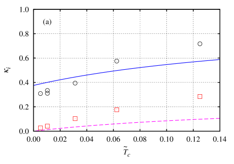
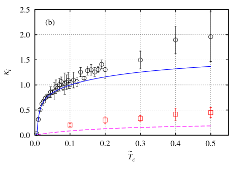
Figure 1: Spatial increment $\kappa_{i}$ of CBSBS obtained from stochastic simulations of (3)-(III) compared with the sum of increments $\kappa_{B}+\kappa_{\sigma}$ (obtained by solving (16) and (III)). The scaled damping rate $\mu=5.12$ is used (e.g. it corresponds to $\nu_{ia}=0.01,\ F=8$). (a) $3D$ simulations with $c_{s}/c=0$, $\tilde{I}=2$ (circles) and $\tilde{I}=1$ (squares). The scaled dimensionless laser intensity $\tilde{I}$, $\mu$ and the scaled correlation time $\tilde{T}_{c}$ are defined in (8). Solid and dashed lines show $\kappa_{B}+\kappa_{\sigma}$ for $\tilde{I}=2$ and $\tilde{I}=1$, respectively. If $\kappa_{\sigma}<0$ then $\kappa_{B}+\kappa_{\sigma}$ is replaced by $\kappa_{B}$. (b) $2D$ simulations with the modified boundary conditions, $c/c_{c}=500$, $\tilde{I}=3$ (circles) and $\tilde{I}=1$ (squares). Error bars are also shown. Solid and dashed lines show $\kappa_{B}+\kappa_{\sigma}$ for $\tilde{I}=3$ and $\tilde{I}=1$, respectively, for both (a) and (b). The details of simulation method are provided in Section V.

Figures 1 show the increment $\kappa_{i}$ of the spatial growth of backscattered light intensity $\langle|B|^{2}\rangle\propto e^{-2\kappa_{i}z}$ as a function of the rescaled correlation time $\tilde{T}_{c}$ obtained from the numerical solution of the stochastic linear equations (3)-(III) (details of numerical simulations are provided in Section V), the scaled damping rate $\mu$ and the scaled laser intensity $\tilde{I}$. These scaling quantities are defined as

$$\tilde{T}_{c}\equiv T_{c}k_{0}c_{s}/4F^{2},\ \mu\equiv 2\nu_{ia}k_{0}^{2}/k_{m}^{2},\ \tilde{I}\equiv\frac{4F^{2}}{\nu_{ia}}\frac{n_{e}}{n_{c}}I.$$ (8)

Here $\tilde{T}_{c}$ has the meaning of the correlation time $T_{c}$ in units of the acoustic transit time along speckle. (Note that definition of $\tilde{T}_{c}$ is different by a factor $1/2F$ from the definition used for FSBS LushnikovRosePRL2004 ; LushnikovRosePlasmPhysContrFusion2006 , where units of the transverse acoustic transit time through speckle were used.) We use dimensionless units with $k_{0}/k_{m}^{2}=4F^{2}/k_{0}$ as the unit in $z$ direction, and $k_{0}/k_{m}^{2}c_{s}$ is the time unit. $\langle\ldots\rangle$ means averaging over the statistics of laser beam fluctuations (II). $\mu$ is the damping rate in units of the inverse acoustic propagation time along a speckle. (See also Figure 4 below for illustration of intensity normalization in comparison with physical units.)

We relate $\kappa_{i}$ to the instability increments for $\langle B\rangle$ and $\langle\sigma^{*}\rangle$ (we designate them $\kappa_{B}$ and $\kappa_{\sigma}$, respectively). In general, growth rates of mean amplitudes give a lower bound to $\kappa_{i}$. However, according to Figure 2, $\sigma$ is almost coherent on a time scale $T_{c}$ justifying the use of mean values of amplitudes.

First we look for the expression for $\kappa_{\sigma}$. Eq. (3) is linear in $B$ and $E$ implying that $B$ can be decomposed into $B=\sum_{j}B_{{\bf k}_{j}}$ with

$$R_{BB}^{-1}B_{{\bf k}_{j}}=\frac{k_{0}}{4}\frac{n_{e}}{n_{c}}\sigma^{*}E_{{\bf k}_{j}}.$$ (9)

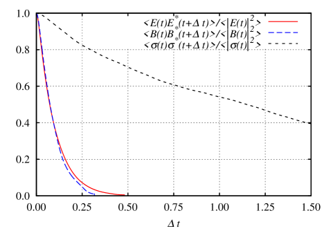
Figure 2: Normalized autocorrelation functions vs. a dimensionless time shift $\Delta t$ for $E,\ B$ and $\sigma$: $\langle E({\bf r},z,t)E^{*}({\bf r},z,t+\Delta t)\rangle$, $\langle B({\bf r},z,t)B^{*}({\bf r},z,t+\Delta t)\rangle$ and $\langle\sigma({\bf r},z,t)\sigma^{*}({\bf r},z,t+\Delta t)\rangle$ with $\tilde{I}=3,$ $\tilde{T}_{c}=0.1$ and $\mu=5.12$ from stochastic simulations of (3)-(III). It is seen that $B$ is correlated at the same time $\tilde{T}_{c}$ as $E$ while $\rho$ is correlated at much larger times.

Approximating r.h.s. of (II) as $E^{*}B\simeq\sum_{j}E_{{\bf k}_{j}}^{*}B_{{\bf k}_{j}}$ gives

$$R_{\sigma\sigma}^{-1}\sigma^{*}=-2k_{0}\sum_{j}E_{{\bf k}_{j}}^{*}B_{{\bf k}_{j}},$$ (10)

which means that we neglect off-diagonal terms $E_{{\bf k}_{j}}^{*}B_{{{\bf k}_{j}}^{\prime}},\quad j\neq j^{\prime}.$ Since speckles of laser field arise from interference of different Fourier modes, $j\neq j^{\prime},$ we associate the off-diagonal terms with speckle contribution to BSBS RoseDuBois1993 ; RosePhysPlasm1995 ; RoseMounaixPhysPlasm2011 . Neglecting off-diagonal terms requires that during time $T_{c}$ light travels much further than a speckle length, $L_{speckle}\ll cT_{c}$ and that $T_{c}\ll t_{sat}$, where $t_{sat}$ is the characteristic time scale at which BSBS convective gain saturates at each speckle MounaixPRL2000 .

Eqs. (9) and (10) result in

$$R_{\sigma\sigma}^{-1}\langle\sigma^{*}\rangle=-(k_{0}^{2}/2)(n_{e}/n_{c})\langle\sum_{j}E_{{\bf k}_{j}}^{*}R_{BB}\sigma^{*}E_{{\bf k}_{j}}\rangle$$ (11)

with the Fourier transformed $R_{BB}$ given by

$$\hat{R}_{BB}({\bf k},z,t)=-ic\delta(z+ct)\exp{[i\frac{k^{2}}{2k_{0}}z]\Theta(-z)},$$ (12)

where $\Theta(z)$ is the Heaviside step function.

We assume that $\sigma^{*}$ is slow in comparison with $E_{{\bf k}_{j}}$ (consistent with Figure 2) which allows to approximate fluctuating terms in r.h.s. of (11) as $\langle E_{{\bf k}_{j}}^{*}\sigma^{*}E_{{\bf k}_{j}}\rangle\simeq\langle\sigma^{*}\rangle\langle E_{{\bf k}_{j}}^{*}E_{{\bf k}_{j}}\rangle$ which has the same form as the Bourret approximation PesmeBerger1994 and provides the closed expression for $\langle\sigma^{*}\rangle$ as follows

$$R_{\sigma\sigma}^{-1}\langle\sigma^{*}({\bf r},z,t)\rangle=-(k_{0}^{2}/2)(n_{e}/n_{c})\int\int\int d{\bf r}^{\prime}dz^{\prime}dt^{\prime}$$

$$\times R_{BB}({\bf r}-{\bf r}^{\prime},z-z^{\prime},t-t^{\prime})C^{*}({\bf r}-{\bf r}^{\prime},z-z^{\prime},t-t^{\prime})$$

$$\times\langle\sigma^{*}({\bf r}^{\prime},z^{\prime},t^{\prime})\rangle,$$ (13)

where the kernel of the response function $R_{BB}({\bf x},z,t)$ is the inverse Fourier transform of (12) and the laser beam correlation function $C$ is given by

$$C({\bf r}-{\bf r}^{\prime},z-z^{\prime},t-t^{\prime})\equiv\langle E({\bf r},z,t)E^{*}({\bf r}^{\prime},z^{\prime},t^{\prime})\rangle$$

$$=\sum_{j}|E_{{\bf k}_{j}}|^{2}\exp\Big{[}i{\bf k}_{j}\cdot({\bf r}-{\bf r}^{\prime})-i\frac{{\bf k}_{j}^{2}}{2k_{0}}(z-z^{\prime})$$

$$-\big{|}t-t^{\prime}-(z-z^{\prime})/c\big{|}/T_{c}\Big{]}$$ (14)

for the top hat model (II),(6) and (III).

We look for solution of (III) in exponential form $\langle\sigma^{*}\rangle\propto e^{i(\kappa z+{\bf k}\cdot{\bf r}-\omega t)}$, then the exponential time dependence of (III) allows to carry all integrations in (12) and (III) explicitly to arrive at the following dispersion relation in dimensionless units

$$-i\omega+\mu+i\kappa-(i/4)k^{2}\qquad\qquad\qquad\qquad\qquad\qquad$$

$$=8iF^{4}\frac{n_{e}}{n_{c}}\sum\limits_{j=1}^{N}\frac{|E_{{\bf k}_{j}}|^{2}}{\omega\frac{c_{s}}{c}+\kappa-k_{j}^{2}-\frac{k^{2}}{2}-{\bf k}_{j}\cdot{\bf k}+2i\frac{c_{s}}{c}\frac{1}{\tilde{T}_{c}}},$$ (15)

where vectors ${\bf k}_{j}$ span top hat (II),(6), and $I=\sum_{j}|E_{{\bf k}_{j}}|^{2}$.

In the continuous limit $N\to\infty$, sum in (III) is replaced by integral, giving for the most unstable mode ${\bf k}=0$:

$$\Delta_{\sigma}(\omega,\kappa) =-i\omega+\mu+i\kappa$$ (16)

$$+i\frac{\mu}{4}\tilde{I}\ln\frac{1-\kappa-\omega\frac{c_{s}}{c}-2i\frac{c_{s}}{c}\frac{1}{\tilde{T}_{c}}}{-\kappa-\omega\frac{c_{s}}{c}-2i\frac{c_{s}}{c}\frac{1}{\tilde{T}_{c}}}=0,$$

which supports the convective instability with the increment $\kappa_{\sigma}\equiv Im(\kappa)>0$ only for $\tilde{I}>\tilde{I}_{convthresh}$, where $\tilde{I}_{convthresh}$ is the convective CBSBS threshold given by

$$\tilde{I}_{convthresh}=\frac{4}{\pi}\Big{(}1-\frac{8c_{s}}{\pi c\tilde{T}_{c}}\Big{)}^{-1}.$$ (17)

In the limit $c/c_{s}\to\infty$, the increment $\kappa_{\sigma}$ is independent of $\tilde{T}_{c}$ which suggests that we refer to it as the collective instability branch. For finite but small $c_{s}/c\ll 1$ and $\tilde{I}>\tilde{I}_{convthresh}$ there is sharp transition of $\kappa_{\sigma}$ as a function of $\tilde{T}_{c}$ from 0 for $\tilde{T}_{c}=0$ to $\tilde{T}_{c}$-independent value of $\kappa_{\sigma}$. That value can be obtained analytically from (16) for $I$ just above the threshold as follows: $\kappa_{\sigma}=\mu(\pi/4-2\tilde{T}_{c}^{-1}c_{s}/c)(\tilde{I}-\tilde{I}_{convthresh})/(\mu\tilde{I}-1)$ absolutecomment .

The increment $\kappa_{B}$ is obtained in a similar way by statistical averaging of equation (3) for $\langle B\rangle$ which gives

$$R_{BB}^{-1}\langle B\rangle=-(k_{0}^{2}/2)(n_{e}/n_{c})\langle ER_{\sigma\sigma}E^{*}B\rangle$$ (18)

with the Fourier transformed response function

$$\hat{R}_{\sigma\sigma}({\bf k},z,t)=-ic_{s}\delta(z-c_{s}t)\exp{[(i\frac{k^{2}}{4k_{0}}-2\nu_{ia}k_{0})z]\Theta(z)}$$ (19)

Then the Bourret approximation (18) results in the following closed expression for $\langle B\rangle$:

$$R_{BB}^{-1}\langle B({\bf r},z,t)\rangle=-(k_{0}^{2}/2)(n_{e}/n_{c})\int\int\int d{\bf r}^{\prime}dz^{\prime}dt^{\prime}$$

$$\times R_{\sigma\sigma}({\bf r}-{\bf r}^{\prime},z-z^{\prime},t-t^{\prime})C^{*}({\bf r}-{\bf r}^{\prime},z-z^{\prime},t-t^{\prime})$$

$$\times\langle B({\bf r}^{\prime},z^{\prime},t^{\prime})\rangle,$$ (20)

where the kernel of the response function $R_{\sigma\sigma}({\bf x},z,t)$ is the inverse inverse Fourier transform of (19) and $C$ is given by (III).

We look for solution of (III) in exponential form $\langle B\rangle\propto e^{i(\kappa z+{\bf k}\cdot{\bf r}-\omega t)}$, then the exponential time dependence of (III) allows to carry all integrations in (19) and (III) explicitly to arrive at the following dispersion relation in dimensionless units

$$\Delta_{B}(\omega,\kappa)=i\omega\frac{c_{s}}{c}+i\kappa$$

$$\qquad\qquad\qquad\qquad\qquad+i\frac{\mu}{4}\tilde{I}\frac{1}{\kappa-\omega-i\mu-i\frac{1}{\tilde{T}_{c}}}=0.$$ (21)

Here we neglected the contribution to $\kappa_{B}\equiv Im(\kappa)$ from diffraction and used the condition $c_{s}/c\ll 1.$ Equation (III) does not have a convective threshold (provided we neglect here light wave damping) while $\kappa_{B}$ has near-linear dependence on $\tilde{T}_{c}:$ $\kappa_{B}\simeq\mu\tilde{I}\tilde{T}_{c}/4$ for $\tilde{T}_{c}<1/\mu$ which is typical for RPA results. It suggests that we refer $\kappa_{B}$ as the RPA-like branch of instability.

Solving the equations (16) and (III) numerically for $\kappa$ allows to find $\kappa_{\sigma}$ and $\kappa_{B}$, respectively, for given $\omega$. We choose $\omega=0.5$ in (16) and $\omega=0$ in (III) to maximize $\kappa_{\sigma}$ and $\kappa_{B}$, respectively. Figures 1a and 1b show that the analytical expression $\kappa_{B}+\kappa_{\sigma}$ is a reasonably good approximation for numerical value of $\kappa_{i}$ above the convective threshold (17) for $\tilde{T}_{c}\lesssim 0.1$ which is the main result of this paper. Below this threshold analytical and numerical results are only in qualitative agreement and we replace $\kappa_{B}+\kappa_{\sigma}$ by $\kappa_{B}$ because $\kappa_{\sigma}<0$ in that case.

The qualitative explanation why $\kappa_{B}+\kappa_{\sigma}$ is a surprisingly good approximation to $\kappa_{i}$ is based on the following argument. First imagine that $B$ propagates linearly and not coupled to the fluctuations of $\sigma^{*}$, so its source is $\sigma^{*}E\to\langle\sigma^{*}\rangle E$ in r.h.s of (3). If $\langle\sigma^{*}\rangle\propto e^{\kappa_{\sigma}z}$ grows slowly with $z$ (i.e. if $\langle\sigma^{*}\rangle$ changes a little over the speckle length $L_{speckle}$ and time $T_{c}$), then so will $\langle|B|^{2}\rangle$ at the rate $2\kappa_{\sigma}$. But if the total linear response $R_{BB}^{tot}$ ($R_{BB}^{tot}$ is the renormalization of bare response $R_{BB}$ due to the coupling in r.h.s of (3)) is unstable then its growth rate gets added to $\kappa_{\sigma}$ in the determination of $\langle|B|^{2}\rangle$ since in all theories which allow factorization of 4-point correlation function into product of 2-point correlation functions, $\langle B(1)B^{*}(2)\rangle=R^{tot}_{BB}(1,1^{\prime})S(1^{\prime},2^{\prime})R^{tot\,*}_{BB}(2^{\prime},2)$. Here $S(1,2)\equiv\langle\sigma^{*}(1)\sigma(2)\rangle\langle E(1)E^{*}(2)\rangle\simeq\langle\sigma^{*}(1)\rangle\langle\sigma(2)\rangle\langle E(1)E^{*}(2)\rangle$ and $``1",\,``2"$ etc. mean a set of all spatial and temporal arguments.

IV Convective instability versus absolute instability

In this Section we show that the dispersion relations (16) and (III) predict absolute instability for large intensities. We first consider the dispersion relation (16) which has branch cut in the complex $\kappa$-plane connecting two branch points $\kappa_{1}=1-\omega\frac{c_{s}}{c}-2i\frac{c_{s}}{c}\frac{1}{\tilde{T}_{c}}$ and $\kappa_{2}=-\omega\frac{c_{s}}{c}-2i\frac{c_{s}}{c}\frac{1}{\tilde{T}_{c}}$.

Absolute instability occurs if the contour $Im(\omega)=const$ in the complex $\omega$-plane cannot be moved down to real $\omega$ axis because of pinching of two solutions of (16) in the complex $\kappa$-plane Briggs1964 ,PitaevskiiLifshitzPhysicalKineticsBook1981 . To describe instability one of these solutions must cross the real axis in $\kappa$-plane as the contour $Im(\omega)=const$ is moving down. The pinch occurs provided

$$\frac{\partial\Delta_{\sigma}(\omega,\kappa)}{\partial\kappa}=0.$$ (22)

The pinch condition (22) together with the requirement of crossing the real axis in $\kappa$-plane result in

$$\kappa=\frac{1}{2}+\frac{1}{2}i\sqrt{\mu\tilde{I}-1}-\frac{c_{s}}{c}{\omega}-\frac{c_{s}}{c}{\frac{2i}{\tilde{T}_{c}}}.$$ (23)

Taking (23) together with $\Delta_{\sigma}(\omega,\kappa)=0$ from (16) at the absolute instability threshold $Im(\omega)=0$ gives the transcendental expression

$$\mu-\frac{1}{2}(\mu\tilde{I}_{absthresh}-1)^{1/2}+\frac{c_{s}}{c}{\frac{2}{\tilde{T}_{c}}}$$

$$-\frac{1}{2}\mu\tilde{I}_{absthresh}\arctan{}\left[(\mu\tilde{I}_{absthresh}-1)^{-1/2}\right]=0$$ (24)

for the absolute instability threshold intensity $\tilde{I}_{absthresh}$. Assuming $\mu\tilde{I}_{absthresh}\gg 1$ we obtain from (IV) the explicit expression for the CBSBS absolute instability threshold

$$\tilde{I}_{absthresh}=\mu+3\mu^{-1}+O(\mu^{-3})+O(\tilde{T}_{c}^{-1}c_{s}/c).$$ (25)

The absolute instability threshold for the second RPA-like branch (III) is obtained similarly with the pinch condition $\frac{\partial\Delta_{B}(\omega,\kappa)}{\partial\kappa}=0.$ It gives the absolute instability threshold for RPA-like branch of instability

$$\tilde{I}_{absthresh,B}=\mu\left(1+\frac{1}{\mu\tilde{T}_{c}}\right)^{2}.$$ (26)

For $\tilde{T}_{c}\lesssim 1$, the threshold (25) is lower than (26) thus (26) can be ignored.

For $\mu\gg 1$ the absolute threshold (25) reduces to the coherent absolute BSBS instability threshold

$$\tilde{I}_{absthreshcoherent}=\mu.$$ (27)

For typical experimental condition $\mu\gtrsim 5$. Then the absolute instability threshold (25) is significantly above the convective instability threshold (17). Thus in simulations described below we emphasize the convective regime and assume $\tilde{I}$ to be below the absolute threshold.

V Numerical simulations

We performed two types of simulations. First type is $3+1D$ simulations (three spatial coordinates $\bf r$, $z$ and $t$) of Eqs. (3), (II) and (III) with the boundary and initial conditions (II),(6) in the limit $c\to\infty$ (i.e., setting $c^{-1}=0$ in (3) and (II)). It implies that the phases $\phi_{{\bf k}_{j}}(t-z/c)$ in (III) become only $t$-dependent, $\phi_{{\bf k}_{j}}(t)$. That formal limit $c\to\infty$, is consistent provided $cT_{c}\gg L_{speckle}$. Then in the linear instability regime, the laser field, $E$, at any time may be obtained by propagation from $z=0$ while the scattered light field, $B$ is obtained by backward propagation from $z=L_{z}$. Time scales are now set by the minimum of $T_{c}$ and the acoustic time scale for the density $\sigma^{*}$. We performed numerical simulation of $B$ and $\sigma^{*}$ via a split-step (operator splitting) method. $E$ advances only due to diffraction and is determined exactly by (III). For given $\sigma^{*}$, $B$ is first advanced due to diffraction in transverse Fourier space, and then the source term (r.h.s. of (3) which is $\propto\sigma^{*}E$) is added for all ${\bf r}=(x,y)$. The density $\sigma^{*}$ is evolved in the strong damping approximation in which the $d/dz$ term is omitted from equation (II). In the regimes of interest, in particular near the collective threshold (17) regime, the dimensionless damping coefficient in (II) increases with acoustic Landau damping coefficient, and even for its physically smallest value of $0.01$, the scaled damping $\mu$ is approximately $5$ while $d/dz$ is either $\simeq\kappa_{i}$ or $1/10$ (an inverse speckle length). So given $E$ and $B$, $\sigma^{*}$ may be advanced in time at each $z$, for each transverse Fourier mode, or since the transverse Laplacian term is estimated as unity in magnitude (base on the speckle width estimate of $F\lambda_{0}$), $\sigma^{*}$ may be approximately advanced at each spatial lattice point.

Second type is $2+1D$ simulations (two spatial coordinates $x$, $z$ and $t$) of Eqs. (3),(II) and(III) with finite value $c_{s}/c=1/500$ (the typical value for the experiment) and modified top-hat boundary condition

$$|E_{\bf k}|=k^{1/2}\,const,\ k<k_{m};\ E_{\bf k}=0,\ k>k_{m},$$ (28)

chosen to mimic the extra factor $k$ in the integral over transverse direction of the full $3+1D$ problem. That modified top hat choice ensures that the linearized equations of that $2+1D$ problem give exactly the same analytical solutions (16) and (III) as for the full $3+1D$ problem. We used again the split step method by integrating along the characteristics of $\rho$ and $B$ and solving for the diffraction by Fourier transform in the transverse coordinate $x$.

We run simulations in the box $0<z<L_{z}$. For both types of simulations the boundary conditions for $B$ were set at $z=L_{z}$. We take these boundary conditions as the Fourier modes of $B({\bf r},z=L_{z},t)$ in $\bf r$ with random time-independent phases. These modes correspond to the random seed from the thermal fluctuations. The boundary conditions for $\rho$ were set to be zero. As the time progress from the beginning of each simulation, both $|\rho|$ and $|B|^{2}$ grow until reaching the statistical steady state if the $\tilde{I}$ is below the threshold of absolute instability (25). Figure 3 shows a typical time dependence of $\langle|B|^{2}\rangle_{x}$, where $\langle\ldots\rangle_{x}$ means averaging over the transverse coordinate $x$. Because we solve linear equations (3) and (II), the maximum value of $\langle|B|^{2}\rangle_{x}$ grows if we increase $L_{z}$ as well as the boundary condition $B({\bf r},z=L_{z},t)$ is defined up to the multiplication by the arbitrary constant. $z$-dependence of $\langle|B|^{2}\rangle_{x}$ in the statistical steady state follows the exponential law $\langle|B|^{2}\rangle_{x}\propto e^{-2\kappa_{i}z}$ well inside the interval $0<z<L_{z}$. Near the boundaries $z=0$ and $z=L_{z}$ there are short transition layers before solution settles at $e^{-2\kappa_{i}z}$ law inside that interval. The particular form of the boundary conditions for $B$ and $\rho$ affect only these transition layers while $e^{-2\kappa_{i}z}$ law is insensitive to them.

To recover $\kappa_{i}$ with high precision we performed simulations for long time after reaching statistical steady state and average $\langle|B|^{2}\rangle_{x}$ over that time at each $z$ (i.e. we assumed ergodicity). E.g. for $\tilde{T}_{c}=0.1$ (the time the laser light travels along $\simeq 5$ laser speckles) we use 256 transverse Fourier modes and discrete steps $\Delta z=0.15$ in dimensionless units with the typical length of the system $L_{z}=50$ ($\simeq 5$ speckle lengths) and a time step $\Delta t=\Delta zc_{s}/c$. For this particular set of parameters it implies $\Delta t=3\cdot 10^{-4}$. For simulation we typically wait $\sim 10^{5}-10^{6}$ time steps to achieve a robust statistical steady state and then average over another $\sim 10^{5}-10^{6}$ time steps (together with averaging over the transverse coordinates) to find $\kappa_{i}$ with high precision. Figures 1a and 1b show $\kappa_{i}$ extracted from $3+1D$ and $2+1D$ simulations, respectively.

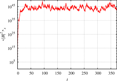
Figure 3: The time dependence of $\langle|B|^{2}\rangle_{x}$ for $3+1D$ simulation with $L_{z}=50$, $\mu=5.12$, $\tilde{T}_{c}=0.1$ and $\tilde{I}=3.0$. $\langle|B|^{2}\rangle_{x}$ is shown at $z=25$. It is seen that after the initial growth, $\langle|B|^{2}\rangle_{x}$ settles at the statistical steady state with the large fluctuations around it. The boundary condition at $z=L_{z}$ is $\langle|B|^{2}\rangle_{x}\sim 1$.

For the practical purposes it is also interesting to estimate the time $t_{ini}$ at which the initial thermal fluctuations of $|B|^{2}$ are amplified by $\sim e^{20}$ to reach the comparable intensity with the laser pump. We obtained from simulations that $\tilde{t}_{ini}\sim 0.7$ for $L_{z}\simeq$ two laser speckles (relevant for gold plasma in ICF experiments and corresponds to $L_{z}\simeq 22$ in dimensionless units), $\tilde{I}=3$ and $\tilde{T}_{c}=0.1$. In dimensional units for NIF conditions $t_{ini}\sim 20$ps which is well below hydrodynamic time (several hundreds of ps).

Figure 2 shows normalized autocorrelation functions $\langle E({\bf r},z,t)E^{*}({\bf r},z,t+\Delta t)\rangle$, $\langle B({\bf r},z,t)B^{*}({\bf r},z,t+\Delta t)\rangle$ and $\langle\sigma({\bf r},z,t)\sigma^{*}({\bf r},z,t+\Delta t)\rangle$ for $\tilde{T}_{c}=0.1$. It is seen that the correlation times for $E$ and $B$ are similar while the correlation time for $\sigma$ is much larger, the more so the smaller $\tilde{T}_{c}$. This justify the use the analytical approximations of the Section III.

VI Applicability of the dispersion relation and estimates for experiment

The applicability conditions of the Bourret approximation used in derivation of (16) and (III) in the dimensionless units are

$$\Delta\omega_{B}\Delta\omega_{\sigma}\gg\gamma_{0}^{2}.$$ (29)

and $\Delta\omega_{B}\gg(c/c_{s})|\kappa_{B}|$ as well as $\Delta\omega_{\sigma}\gg\mu$. Here $\gamma_{0}$ is the temporal growth rate of the spatially homogeneous solution given by $\gamma_{0}^{2}=(1/4)(c/c_{s})\mu\tilde{I}.$ Also $\Delta\omega_{\sigma}=1/\tilde{T}_{c}$ is the bandwidth for $\sigma$ and $\Delta\omega_{B}$ is the effective bandwidth for $B$. $\Delta\omega_{B}$ is dominated by the diffraction in (3) giving in the dimensionless units $\Delta\omega_{B}=c/c_{s}$. Then (29) reduces to $\tilde{T}_{c}\ll 4/(\mu\tilde{I})$ and $|\kappa_{B}|\ll 1$. Together with the condition $T_{c}\gg L_{speckle}/c$ used in the derivation of (16) and assuming that $\tilde{I}\simeq\tilde{I}_{convthresh}$, it gives a double inequality $(7\pi/2)(c_{s}/c)\ll\tilde{T}_{c}\ll\pi/\mu$ which can be well satisfied for $\mu\simeq 5$, i.e. for $\nu_{ia}\simeq 0.01$ as in gold ICF plasma but not for $\mu\simeq 50$ as in low ionization number $Z$ ICF plasma. Also $|\kappa_{B}|<1$ implies that $\tilde{I}>\tilde{I}_{convthresh}$ because otherwise, below that threshold, $\kappa_{B}\sim-\mu$ which would contradict $|\kappa_{B}|<1$. All these conditions are satisfied for $\tilde{T}_{c}\lesssim 1/4$ for the parameters of Figure 1 with $\tilde{I}=2$ or $\tilde{I}=3$ (solid lines in Figure 1) but not for $\tilde{I}=1$ (dashed lines in Figure 1). Additionally, an estimate for $T_{c}\ll t_{sat}$ from the linear part of the theory of Ref. MounaixPRL2000 results in the condition $\tilde{T}_{c}\ll 8\tilde{I}/\mu$ which is less restrictive than above conditions. These estimates are consistent with the observed agreement between $\kappa_{i}=\kappa_{\sigma}+\kappa_{B}$ and $\kappa_{i}$ from simulations (filled circles in Figures 1) for $\tilde{I}$ above the threshold (17). We conclude from Figures 1 that the applicability condition for the Bourret approximation is close to the domain of $\tilde{T}_{c}$ values for which $\kappa_{i}=\kappa_{\sigma}+\kappa_{B}$.

For nominal NIF parameters Lindl2004 ; LushnikovRosePlasmPhysContrFusion2006 , $F=8,\ \ n_{e}/n_{c}=0.1,\ \lambda_{0}=351\mbox{nm}$, $c_{s}=6\times 10^{7}\ \mbox{cm s}^{-1}$ and electron plasma temperature $T_{e}\simeq 2.6\mbox{keV}$ ($T_{e}$ was recently updated from the old standard value $T_{e}\simeq 5\mbox{keV}$ RosenInvitedAPRPlasma2011 ), we obtain from (17) that $I_{convthresh}\simeq 1.1\times 10^{14}\mbox{W}/\mbox{cm}^{2}$ for gold plasma with $\nu_{ia}\simeq 0.01$ which is in the range of NIF single polarization intensities. Fig. 4 shows $\kappa_{i}$ in the limit $c_{s}/c=0,\ \tilde{T}_{c}\to 0$ from simulations, analytical result $\kappa_{\sigma}$ ($\kappa_{B}=0$ in that limit) and the instability increment of the coherent laser beam $\kappa_{coherent}=\mu/2-(\mu^{2}-\mu\tilde{I})^{1/2}/2$ (see e.g. Kruer1990 ). It is seen that the coherent increment significantly overestimates numerical increment especially around $I_{convthresh}.$ The convective increment $\kappa_{i}$ has a significant dependence on $\tilde{T}_{c}$ if we include the effect of finite $c/c_{s}=500$ and finite $\tilde{T}_{c}$ as in Fig. 1b. Current NIF 3Å beam smoothing design has $T_{c}\simeq 4$ps implying $\tilde{T}\simeq 0.15$. In that case Fig. 1b shows that there is a significant (about 5 fold) change in $\kappa_{i}$ between $\tilde{I}=1$ and $\tilde{I}=3$. Similar estimate for KrF lasers ($\lambda_{0}=248\mbox{nm},\ F=8,\ T_{c}=0.7$ps) gives $\tilde{T}_{c}=0.04$ which results in a significant ($40\%$) reduction of $\kappa_{i}$ for $\tilde{I}=3$ compare with above NIF estimate.

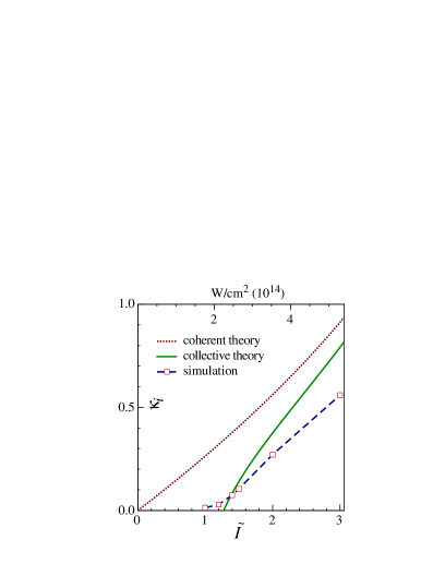
Figure 4: $\kappa_{i}$ vs. $\tilde{I}$ for $\mu=5.12$ obtained from $3+1D$ simulations (squares connected by dashed line, $c_{s}/c=0$ and limit $\tilde{T}_{c}\to 0$ taken by extrapolation from $\tilde{T}_{c}\ll 1$), analytical result $\kappa_{\sigma}$ (solid curve) and coherent laser beam increment $\kappa_{coherent}$ (dotted curve). The scaled dimensionless laser intensity $\tilde{I}$ and damping rate $\mu$ in units of acoustic propagation time along a speckle are defined in (8). Upper grid corresponds to laser intensity in dimensional units $I_{physical}\propto T_{e}/\lambda_{0}^{2}$ for NIF parameters and gold plasma $T_{e}\simeq 5\mbox{keV},\ F=8,\ \ n_{e}/n_{c}=0.1,\nu_{ia}=0.01,\ \lambda_{0}=351\mbox{nm}$.

The BSBS threshold may be reduced by self-induced temporal incoherence (see e.g. SchmittAfeyan1998 ), which in its linear regime, includes collective FSBS (CFSBS) which reduces $T_{c}$ and laser correlation lengths. For low $Z$ plasma, the CBSBS and CFSBS thresholds are close while the latter may be lowered by adding higher $Z$ dopant.

VII Conclusion

In conclusion, we identified the collective threshold (17) of BSBS instability of partially incoherent laser beam for ICF relevant plasma. Above that threshold the CBSBS increment $\kappa_{i}$ is well approximated by the sum of the collective-like increment $\kappa_{\sigma}$ and RPA-like increment $\kappa_{B}$. That result is in agreement with the direct stochastic simulations of BSBS equations. Values of $\kappa_{\sigma}$ and $\kappa_{B}$ are comparable above threshold while in a small neighborhood of threshold the value of $\kappa_{i}$ changes quickly with changing either correlation time or laser intensity to pass through collective threshold. With further increase of laser intensity the absolute instability also develops above the threshold (25).

- (1) J. D. Lindl, et al., Phys. Plasmas 11, 339 (2004).
- (2) N. B. Meezan, et al., Phys. Plasmas 17, 056304 (2010).
- (3) S. H. Glenzer et. al., Nature Phys., 3, 716 (2007); D. H. Froula, et al., Phys. Rev. Lett., 98, 085001 (2007); N. B. Meezan, et al., Phys. Plasmas, 17, 056304 (2010) X. Meng, et al., Phys. Plasmas, High Power Laser Science and Engineering, 1, 94 (2012).
- (4) W. L. Kruer, The physics of laser plasma interactions, Addison-Wesley, New York (1990).
- (5) H. A. Rose, Phys. Plasmas 2, 2216 (1995).
- (6) J. Garnier, Phys. Plasmas 6, 1601 (1999).
- (7) A. A. Vedenov, and L. I. Rudakov, Sov. Phys. Doklady 9, 1073 (1965); A. M. Rubenchik, Radiophys. Quant. Electron. 17, 1249 (1976); V. E. Zakharov, S. L. Musher, and A. M. Rubenchik, Phys. Rep. 129, 285 (1985).
- (8) D. Pesme, et al., Natl. Tech. Inform. Document No. PB92-100312 (1987); arXiv:0710.2195 (2007).
- (9) P. M. Lushnikov and H. A. Rose, Phys. Rev. Lett. 92, 255003 (2004).
- (10) P. M. Lushnikov and H. A. Rose, Plasma Phys. Controlled Fusion 48, 1501 (2006).
- (11) H. A. Rose and D. F. DuBois, Phys. Rev. Lett. 72, 2883 (1994).
- (12) P. M. Lushnikov and H. A. Rose, arXiv:0710.0634 (2007).
- (13) C. Niemann, et al., Phys. Rev. Lett. 100, 045002 (2008).
- (14) The literature is replete with multi-dimensional simulations of SBS, with models which are similar to the one used in our work (see. e.g. SchmittAfeyan1998 ; MassonLabordePesmeEtAlJDePhys2006 ; PesmeEtAlPRL2000 ). However, the other works emphasize nonlinear regimes with competing instabilities, such as BSBS and filamentation, while we apply our theory and simulation to strictly linear BSBS regime.
- (15) H. A. Rose and Ph. Mounaix, Phys. Plasmas 18, 042109 (2011).
- (16) A. Bers, pp. 451-517, In Handbook of plasma physics, Eds. M.N Rosenbluth, at. al., North-Holland (1983).
- (17) L. P. Pitaevskii, and E.M. Lifshitz, Physical Kinetics: Volume 10, Butterworth-Heinemann, Oxford (1981).
- (18) Ph. Mounaix, et al., Phys. Rev. Lett. 85, 4526 (2000).
- (19) D. F. DuBois, B. Bezzerides, and H. A. Rose, Phys. of Fluids B: Plasma Physics 4, 241 (1992).
- (20) R. H. Lehmberg and S. P. Obenschain, Opt. Commun. 46, 27 (1983).
- (21) Subsequent analysis can be easily generalized to include polarization smoothing Lindl2004 .
- (22) H. A. Rose and D. F. DuBois, Phys. of Fluids B5, 3337 (1993).
- (23) M.D. Rosen,et al., High Energy Density Physics 7, 180 (2011).
- (24) This expression is valid for , while for the convective threshold coinsides with the absolute instability threshold.
- (25) A. J. Schmitt and B. B. Afeyan, Phys. Plasmas 5, 503 (1998).
- (26) P.E. Masson-Laborde, et al., J. De Physique IV 133, 247 (2006).
- (27) D. Pesme, et al., Phys. Rev. Lett. 84, 278 (2000); A. V. Maximov, et al., Phys. Plasmas 8, 1319 (2001); P. Loiseau, et al., Phys. Rev. Lett. 97, 205001 (2006).