Study of Critical Dynamics in Fluids via Molecular Dynamics in Canonical Ensemble

Abstract

With the objective of understanding the usefulness of thermostats in the study of dynamic critical phenomena in fluids, we present results for transport properties in a binary Lennard-Jones fluid that exhibits liquid-liquid phase transition. Various collective transport properties, calculated from the molecular dynamics (MD) simulations in canonical ensemble, with different thermostats, are compared with those obtained from MD simulations in microcanonical ensemble. It is observed that the Nosé-Hoover and dissipative particle dynamics thermostats are useful for the calculations of mutual diffusivity and shear viscosity. The Nosé-Hoover thermostat, however, as opposed to the latter, appears inadequate for the study of bulk viscosity.

I Introduction

In the vicinity of a critical point zinn , various static zinn ; stanley ; onuki1 and dynamic onuki1 ; onuki2 ; hohenberg ; ferrell1 ; olchowy ; luettmer ; anisimov ; burstyn1 ; burstyn2 quantities exhibit power-law singularities. Computer simulations played a crucial role in the understanding of static critical phenomena landau . In dynamics, on the other hand, simulations are recent, particularly for fluid criticality. In this case, in addition to the finite-size effects, critical slowing down poses enormous difficulty. Note that the slowest relaxation time, $\tau_{{}_{max}}$, diverges at the criticality as onuki1 ; landau

$$\tau_{{}_{max}}\sim L^{z},$$ (1)

where $L$ is the linear dimension of the system and $z$ is a dynamic critical exponent. While in the static critical phenomena, the problem of critical slowing down can be significantly reduced via a smart choice of ensemble (with smaller value of $z$ ), in dynamics this is not possible. The liberty in statics stems from the robust universality of static critical phenomena.

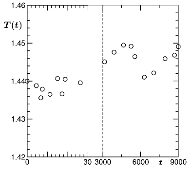
Figure 1: Drift of temperature is demonstrated for a typical molecular dynamics run in microcanonincal ensemble. The chosen temperature is very close to the critical value. The cubic simulation box has a linear dimension $L=14$ and number of particles $2744$. The initial temperature is set to a value $1.44$.

For the computational study of critical dynamics in fluids, using microscopic models, one typically carries out molecular dynamics (MD) frenkel ; allen ; rapaport simulations. Usually one considers the microcanonical ensemble (constant N, V, E, which are respectively the total number of particles, confining volume and energy) where requirements of hydrodynamics are satisfied. However, as seen in Eq. (1), close to the critical point, overwhelmingly long simulation runs are required to avoid finite-size effects even at a moderate level. In such a situation, control of temperature ($T$) in the NVE ensemble becomes problematic. A representative case for temperature drift in microcanonical runs has been shown in Fig. 1. Drift of such magnitude is acceptable in the normal region of the parameter space, i.e., far away from any phase transition. However, close to the critical point, where one focuses on quantifying singular behavior, this becomes problematic. This calls for the study of fluid critical dynamics in canonical (NVT) ensemble where, instead of $E$, $T$ is kept constant.

Various thermostats frenkel ; allen are used to maintain temperature in MD simulations in NVT ensemble, e.g. Andersen thermostat (AT), Langevin thermostat (LT), Nosé-Hoover thermostat (NHT), dissipative particle dynamics thermostat (DPDT), etc. Even though most of the thermostats are useful in controlling the temperature of the system, only a few are appropriate for the calculation of transport properties in fluids. Crucial tests of a thermostat, in terms of providing the correct value of a transport quantity as well as in keeping the temperature constant, lie in nontrivial phenomena like phase transition dynamics. In a recent work roy2014 , we have demonstrated the usefulness of the NHT for the calculation of shear viscosity. In this paper we address this issue in a more general context.

In AT frenkel , the temperature is controlled via the random assignments of velocities to a fraction of particles according to the Maxwell distribution, mimicking collisions of the particles with a heat bath. Due to this Monte Carlo-like stochastic nature, AT is not useful for the calculation of transport properties in fluids. With increasing collision frequency, the transport coefficients deviate further and further from the desired value. This stochastic character is also true for LT.

For MD in NVE ensemble, one solves the Newton’s equations of motion involving the inter-particle force. Like AT, in the NVT ensemble, depending upon the thermostat, additional rules are imposed. In the case of LT, an additional drag force proportional to the velocity is introduced, in addition to a random force, both coming from the background solvent particles. There, for the $i$th particle, one solves the equation grest

$$\frac{d^{2}{\vec{r}}_{i}}{dt^{2}}=-\vec{\nabla}U_{i}-\gamma\frac{d{\vec{r}}_{i}}{dt}+{\vec{W}}_{i},$$ (2)

where ${\vec{r}}_{i}$ is the position of the particle, $U_{i}$ is the inter-particle potential, $t$ is the time, $\gamma$ the drag coefficient and ${\vec{W}}_{i}$ is a temperature-dependent Gaussian noise with mean zero. The noise correlation between two times $t$ and $t^{\prime}$ follows the fluctuation-dissipation relation

$$\langle{W_{i\mu}W_{j\nu}}\rangle=2k_{B}T{\gamma}\delta_{ij}\delta(t-t^{\prime})\delta_{\mu\nu}.$$ (3)

In Eq. (3), $\mu$ and $\nu$ correspond to the Cartesian axes of space coordinates and $k_{B}$ is the Boltzmann constant. In case of non-Gaussian noise, one needs to appropriately adjust the numerical factor in Eq. (3). In this work we have used uniform random numbers between $-1$ and $1$, thus the prefactor $2$ is replaced by $6$.

Due to their inability to conserve the local momentum, AT and LT are used only for the equilibration purpose. Nevertheless, for the sake of completeness, we will present some results using these thermostats as well. But, there exist a number of thermostats, e.g. NHT, DPDT, etc., that are believed to be good for the calculation of transport properties in fluids. The understanding of the usefulness of these thermostats, however, to the best of our knowledge, is essentially restricted to the single particle dynamics.

In DPDT stoyanov ; nikunen ; soddemann , the dissipative force in Eq. (2) is given by $\gamma\omega^{D}(r_{ij})({\vec{v}}_{ij}\cdot{\vec{e}}_{ij}){\vec{e}}_{ij}$ where ${\vec{r}}_{ij}$ and ${\vec{v}}_{ij}$ are respectively the relative position and velocity between $i$ and $j$ particles with ${\vec{e}}_{ij}={\vec{r}}_{ij}/{r_{ij}}$; $r_{ij}=|{\vec{r}}_{ij}|=r$. Here, $\omega^{D}$ is a weight function connected to the random force as $\sqrt{2\gamma k_{B}T\omega^{D}}\omega_{ij}{\vec{e}}_{ij}$, where $\omega_{ij}$ are random numbers with $\omega_{ij}=\omega_{ji}$. For the choice of $\omega^{D}$, there is no fixed prescribed rule. In this work we use pastorino $\omega^{D}=(1-r)^{2}$ for $r\leq 1$ and $0$ otherwise. From the property of the random force and the expression of the dissipative force, it is understandable that DPDT will preserve local momentum, thus hydrodynamics. However, this thermostat has issues related to keeping the temperature constant. For the choice of the weight function mentioned above and $\gamma=0.1$, we obtained reasonable temperature control in this work. Note that for LT we used $\gamma=1$.

In NHT, an additional degree of freedom $\Xi$ is introduced and one solves the equations frenkel

$$m_{i}\dot{\vec{r}}_{i}=\vec{p}_{i},$$ (4)

$$\dot{\vec{p}}_{i}=-\frac{\delta U_{i}}{\delta\vec{r}_{i}}-\Xi\vec{p}_{i},$$ (5)

$$\dot{\Xi}=\Big{(}\sum_{i=1}^{N}p_{i}^{2}/m_{i}-3N/\beta\Big{)}/Q,$$ (6)

where $\beta=1/{k_{B}T}$, $\Xi$ is a time dependent drag, $\vec{p}_{i}$ is the momentum and $Q$ is the coupling strength between the system and the thermostat. Essentially, in this case, the simulation is done in microcanonical ensemble frenkel ; stoyanov with a modified Hamiltonian that provides averages equivalent to those of a canonical ensemble with the original Hamiltonian. The original energy function, that is constant in microcanonical ensemble, fluctuates in this method, as in the canonical ensemble. The constant of motion here is related to the Helmholtz free energy. Unless otherwise mentioned, for all our presented results the value of $Q$ was set to unity.

As is clear by now, in this paper we provide results for the utility of NHT and DPDT with respect to the study of dynamic critical phenomena. Despite its problems related to local momentum conservation, NHT still remained popular for the study of transport using NVT ensemble. Of course, every hydrodynamic preserving thermostat has some disadvantages, e.g., DPDT suffers from the temperature control problem.

The rest of the paper is organized as follows. In Section II, we introduce the model. The results are presented in Section III. Finally, the paper is concluded in Section IV with a summary and discussion.

II Model and Phase Behavior

In our binary ($A+B$) mixture model das3 ; das4 ; royepl , particles interact via the Lennard-Jones (LJ) pair potential

$$u(r)=4\varepsilon_{{}_{\alpha\beta}}\Big{[}\Big{(}\frac{\sigma}{r}\Big{)}^{12}-\Big{(}\frac{\sigma}{r}\Big{)}^{6}\Big{]},$$ (7)

where $\sigma$ is the particle diameter and $\varepsilon_{\alpha\beta}~{}[\alpha,\beta=A,B]$ is the interaction strength. For the sake of computational convenience, we have introduced a cut-off and shifting of the potential to zero at $r_{c}=2.5\sigma$. This, however, introduces a discontinuity in the force at $r_{c}$, which was removed by adding a term allen $(r-r_{{}_{c}})({du}/{dr})_{{r}=r_{{}_{c}}}$. We work with a symmetric model by setting $\varepsilon_{{}_{AA}}=\varepsilon_{{}_{BB}}=2\varepsilon_{{}_{AB}}=\varepsilon$ which produces liquid-liquid phase separation. The overall density of particles was set to unity. This avoids overlap between liquid-liquid and vapor-liquid phase separation.

The phase diagram for this model was studied das3 ; das4 ; royepl via a semi grandcanonical Monte Carlo landau ; frenkel method. In this scheme, in addition to the standard particle displacement moves, one tries identity switches $A\rightarrow B\rightarrow A$ which are accepted or rejected according to the standard Metropolis criterion. For the identity moves it is necessary to include in the Boltzmann factor frenkel the chemical potential difference between the two species. This difference, however, is zero along coexistence and for $50:50$ composition above the critical temperature $T_{c}$, due to the symmetry of the model. In this ensemble, from the fluctuation of concentration $x_{\alpha}(=N_{\alpha}/N,$ $N_{\alpha}$ being the number of particles of species $\alpha$), one obtains a probability distribution $P(x_{\alpha})$. Below the critical temperature, $P(x_{\alpha})$ should have a two-peak structure, the locations of the peaks providing the points along the coexistence. At the critical temperature, the form of the distribution crosses over from the double peak to a single peak one. But, this critical temperature is system-size dependent that we will denote as $T_{c}^{L}$, which, in the limit $L\rightarrow\infty$, will converge to the thermodynamic critical temperature, $T_{c}$. In Table I we list the values of $T_{c}^{L}$ for a few system sizes royepl ; royjcp .

As already mentioned, transport properties are studied via MD simulations in NVE as well as NVT ensembles, for the latter various temperature controlling methods, discussed in the previous section, were used. Details on the calculation of transport properties will be provided in the next section.

All our simulations were performed in three space dimensions with cubic boxes of linear size $L$ (in units of $\sigma$) and periodic boundary conditions in all directions. The equations of motion in MD were solved by applying Verlet velocity algorithm with integration time step $\Delta t=0.005$. Before starting the production runs, the configurations were equilibrated via MC simulations and, in the case of MD in NVE ensemble, further thermalization runs were performed via MD with AT. Except for self diffusivity, results are presented after averaging over a very large number of independent initial configurations, ranging between $80$ and $640$. In case of self-diffusivity, this number is $5$. For collective properties, as the terminology suggests, such high numbers become necessary due to lack of averaging involving the individual particles.

Table 1:

$L$	8	10	12	14	16	$\infty$
$T_{c}^{L}$	1.461	1.447	1.440	1.436	1.433	$T_{c}\simeq 1.421$

III Results

Using MD, at various temperatures (fixing the composition to the critical value) we present results for the self diffusivity ($D$), Onsager coefficient ($\mathscr{L}$), shear viscosity ($\eta$) and bulk viscosity ($\zeta$). These quantities were calculated (in dimensionless units) from the Green-Kubo (GK) relations hansen as (note that, because of the symmetry of the model $D=D_{A}=D_{B}$, $D_{\alpha}$ being the self diffusivity of species $\alpha$)

$$D(t)=\Big{(}{\frac{t_{0}}{3\sigma^{2}}}\Big{)}\int_{0}^{t}dt^{\prime}\langle{{\vec{v}}_{i,\alpha}(t^{\prime}){\vec{v}}_{i,\alpha}(0)}\rangle,$$ (8)

$${\mathscr{L}}(t)=\left(\frac{t_{{}_{0}}\varepsilon}{3k_{{}_{B}}NT\sigma^{2}}\right)\int_{0}^{t}dt^{\prime}\langle{{\vec{J}}_{{}_{AB}}}(t^{\prime}){{\vec{J}}_{{}_{AB}}}(0)\rangle,$$ (9)

$$\eta(t)={\left(\frac{t_{{}_{0}}^{3}\varepsilon}{\sigma VTm^{2}}\right)\int_{0}^{t}dt^{\prime}\langle{P_{\mu\nu}}(t^{\prime}){P_{\mu\nu}}(0)\rangle},$$ (10)

and

$$Y(t)={\left(\frac{t_{{}_{0}}^{3}\varepsilon}{\sigma VTm^{2}}\right)\int_{0}^{t}dt^{\prime}\langle{P^{{}^{\prime}}_{\mu\mu}}(t^{\prime}){P^{{}^{\prime}}_{\mu\mu}}(0)\rangle},$$ (11)

where $t_{0}$ is the LJ time unit $(=\sqrt{m\sigma^{2}/\varepsilon})$ and $m$ is the mass (same for all particles in our model). In Eq. (9), ${\vec{J}}_{AB}$ is a concentration current defined as

$${\vec{J}}_{{}_{AB}}(t)={{x_{{}_{B}}}{\sum}_{i=1}^{N_{{}_{A}}}{\vec{v}_{{}_{i,A}}}(t)}-{{x_{{}_{A}}}{\sum}_{i=1}^{N_{{}_{B}}}{\vec{v}_{{}_{i,B}}}(t)},~{}~{}$$ (12)

${\vec{v}}_{{}_{i,\alpha}}$ being the velocity of $i$th particle of species $\alpha$. In Eq. (10), $P_{\mu\nu}$ are the off-diagonal elements of the pressure tensor given as hansen

$$P_{\mu\nu}(t)=\sum_{i=1}^{N}\Big{[}mv_{i\mu}v_{i\nu}+\frac{1}{2}\sum_{j(\neq i)}(\mu_{i}-\mu_{j})F_{\nu}(|{\vec{r}}_{i}-{\vec{r}}_{j}|)\Big{]},~{}~{}~{}~{}~{}$$ (13)

$\vec{F}$ being the force between particles $i$ and $j$; $\mu_{i}$ is a Cartesian coordinate for the position of particle $i$. In Eq. (11), $Y=\zeta+\frac{4}{3}\eta$ and $P^{{}^{\prime}}_{\mu\mu}=P_{\mu\mu}-P$, $P$ being the pressure.

These quantities can also be calculated from the corresponding mean squared displacements (MSD) following the Einstein relations, e.g., the self diffusivity $D$, the Onsager coefficient ${\mathscr{L}}$ and the shear viscosity $\eta$ are calculated as hansen

$$D(t)=\Big{(}\frac{t_{0}}{6t\sigma^{2}}\Big{)}\langle|{\vec{r}}_{i,\alpha}(t)-{\vec{r}}_{i,\alpha}(0)|^{2}\rangle,$$ (14)

and

$${\mathscr{L}}(t)=\left(\frac{{t_{{}_{0}}}N_{A}^{2}\varepsilon}{6k_{{}_{B}}tNT\sigma^{2}}\right)\langle|{\vec{R}}_{{}_{A}}(t)-{\vec{R}}_{{}_{A}}(0)|^{2}\rangle,$$ (15)

and

$$\eta(t)=\left(\frac{t_{{}_{0}}^{3}\varepsilon}{2k_{{}_{B}}tVd_{0}Tm^{2}}\right)\langle|Q_{{}_{xy}}(t)-Q_{{}_{xy}}(0)|^{2}\rangle.$$ (16)

In Eq. (15), ${\vec{R}}_{\alpha}$ is the centre of mass (CM) coordinate of species $\alpha$ and in Eq. (16), the generalized displacement $Q_{xy}$ has the expression

$$Q_{{}_{xy}}(t)=\sum_{i=1}^{N}{x_{{}_{i}}(t)v_{iy}(t)}.$$ (17)

In the rest of the paper, we set $m$, $\varepsilon$, $\sigma$, $t_{0}$ and $k_{B}$ to unity. For self diffusivity, Onsager coefficient and shear viscosity, we present results from the MSD relations whereas the results for bulk viscosity were obtained using the GK relation.

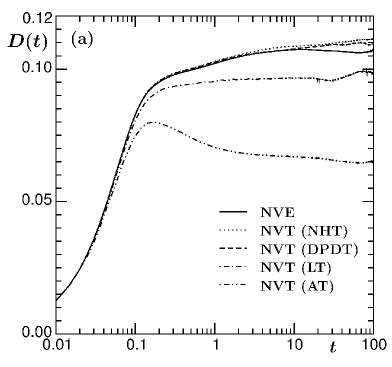
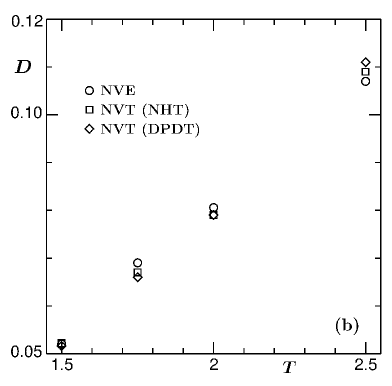
Figure 2: (a) Plot of time dependent self diffusivity obtained using various ensembles. (b) Plot of $D~{}[D(\infty)]$ vs $T$, for NVE, NHT and DPDT. All results are obtained after averaging over $5$ independent initial configurations.

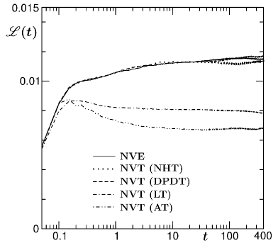
Figure 3: Plot of Onsager coefficient as a function of time, from MD calculations in NVE and NVT ensembles. For NVT ensemble, as indicated, four different thermostats were used. In all the cases, values of T and L were set to $2.5$ and $10$, respectively.

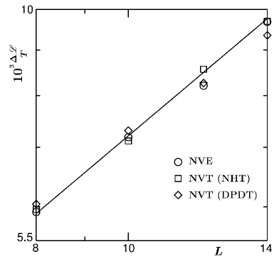
Figure 4: A finite-size scaling plot of Onsager coefficient $[{\mathscr{L}}={\mathscr{L}}(\infty)]$, after subtracting the background contribution, using data at $T_{c}^{L}$s. Results from both NVE and NVT ensembles are shown. For NVT ensemble, we have included data from NHT and DPDT. The continuous line corresponds to the theoretical prediction for critical divergence.

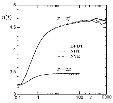
Figure 5: Plot of shear viscosity as a function of time for two different temperatures, viz., $T=2.5$ and $T=1.447$, the latter being the value of $T_{c}^{L}$ for $L=10$, the system size for which the results are presented. We have shown results from NVE, NHT and DPDT calculations.

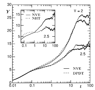
Figure 6: Comparison of time dependent bulk viscosity for calculations from NVE and DPDT, at two different temperatures. The inset shows a comparison between NVE and NHT for this quantity, only at $T=2.5$.

We start by showing a comparison of the time dependent self-diffusivity, calculated from the Einstein relation, in Fig. 2(a), obtained from NVE and NVT ensembles, at $T=2.5$. For NVT ensemble we have included results from AT, LT, NHT and DPDT as temperature controller. As expected, AT and LT do not provide results consistent with the NVE one. However, the results from NHT and DPDT are very much in agreement with the latter. The final values of the transport quantities, here and in other places, are obtained from the flat portions of these time-dependent plots. In Fig. 2(b) we show a comparison of $D$ calculated from NVE, NHT and DPDT, as a function of temperature, along the critical ($50:50$) composition line. All are in good agreement (the observed differences are not systematic). This is expected and demonstrated earlier frenkel . However, the cases of collective properties (except for shear viscosity, via NHT, in a recent work roy2014 ) are missing in the literature which we address below.

In Fig. 3 we show a comparison similar to Fig. 2(a) but for the time-dependent Onsager coefficient. For NHT, even though we have presented the result using only $Q=1$, we have performed the calculations with values of $Q$ up to $100$ and observed that the results are not very sensitive to the choice of this parameter. This fact will be demonstrated later, for all the transport quantities, by presenting representative results using the optimum value nose of $Q$ ($\sim 6Nk_{B}T/\omega_{0}^{2}$, $\omega_{0}$ being a characteristic vibrational frequency whose value is approximately $10$ for typical LJ fluid). Again, very good agreement is observed for results from NVE, NHT and DPDT. In the following we focus on the critical behavior of this quantity.

Note that $\mathscr{L}$ is expected to diverge at criticality with the correlation length $\xi$ as onuki1

$$\frac{\mathscr{L}}{T}\sim\xi^{x_{\lambda}},$$ (18)

with $x_{\lambda}\simeq 0.9$. To verify the consistency of our simulation results with this number for the critical exponent, we take the route of finite-size scaling analysis fisher2 . Noting that at criticality $\xi$ scales with $L$, for results obtained at $T_{c}^{L}$,

$$\frac{\mathscr{L}}{T}\sim L^{x_{\lambda}}.$$ (19)

It was observed in previous NVE MD simulations of this model das3 ; das4 that $\mathscr{L}$ has strong background contribution ${\mathscr{L}}_{b}$. The value of ${\mathscr{L}}_{b}$ was estimated to be $\simeq 0.0033$, a reasonably large number, given that for small system sizes this number can be comparable to the total value. We will thus deal with the critical part $\Delta{\mathscr{L}}(={\mathscr{L}}-{\mathscr{L}}_{b})$ only. So, when calculated at $T_{c}^{L}$s, a plot of $\Delta{\mathscr{L}}/T$ vs $L$ will be consistent with a power-law with exponent $0.9$. This is demonstrated in Fig. 4. Note that we have shown results from NHT, DPDT, as well as from NVE ensemble. All of them are in good agreement. This essentially demonstrates that NHT and DPDT are good devices for the calculation of mutual diffusivity ($D_{AB}$) even for quantitative understanding of critical dynamics. Here note that $D_{AB}={\mathscr{L}}/{\chi}$, where $\chi$ is the concentration susceptibility that can be conveniently calculated from concentration fluctuation in Monte Carlo simulations. Sightly poorer agreement of the DPDT data with the expected theoretical behavior, compared to NHT ones, is due to the temperature control problem that this method suffers from, in the long run.

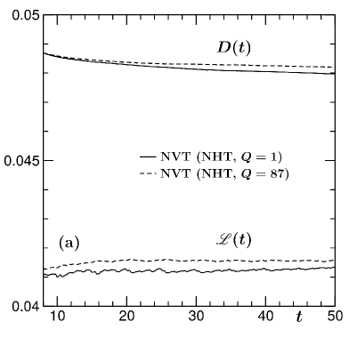
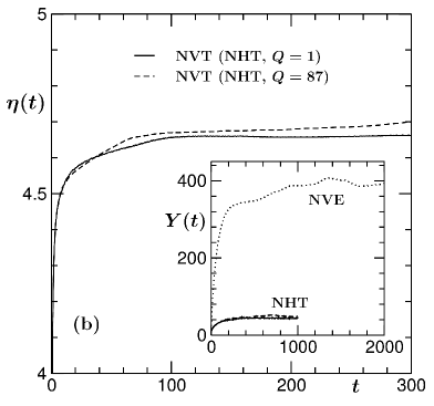
Figure 7: (a) A comparative plot of $D(t)$ and $\mathscr{L}(t)$, obtained using NHT, for two values of $Q$. Results correspond to $L=10$, $T=T_{c}^{L}$. Data for $\mathscr{L}$ has been multiplied by $3$. (b) Same as (a), but for $\eta(t)$ (main frame) and $Y(t)$ (inset).

Having demonstrated the usefulness of NHT and DPDT in the calculation of the diffusion constants, we turn our attention to viscosities. In Fig. 5 we show the time dependent shear viscosity, using the Einstein relation, for NVE, NHT and DPDT. Two different temperatures are included, viz., $T=2.5$ and $T=1.447$. Here we do not show the results obtained using AT and LT which, we have already understood and as is known, are not appropriate for the study of transport properties in fluids. For both NHT and DPDT, satisfactory agreement is achieved with the NVE calculation. In our recent work roy2014 , agreement between the NHT and NVE was established. There our estimations of the corresponding critical exponent via these two methods agreed nicely with each other. However, in this work, DPDT was not applied. Having demonstrated the expected usefulness of DPDT, for this purpose, we move to the case of bulk viscosity. For bulk viscosity we avoid demonstrating the critical divergence, by keeping the difficulty in estimation of this quantity in mind. One of the primary difficulties lies in the estimation of $P$ that needs to be subtracted from the diagonal elements of the pressure tensor. Even a slight error in this quantity can lead to a misleading number in the final value. This, however, in our calculations was appropriately taken care of. Here note again that, for all the collective transport properties discussed in this work, the critical divergences were estimated from calculations via MD in NVE ensembles and the results are in good agreement with existing theoretical predictions. Due to the above mentioned difficulty and diverging relaxation time, it becomes inevitable to choose temperatures reasonably far away from the critical value, for the bulk viscosity.

Even though so far it appears that the NHT is a good tool to study dynamic critical phenomena, in fact better than the DPDT, from the temperature control point of view, we have encountered difficulty in the calculation of bulk viscosity, at least for this value of the coupling constant. In Fig. 6 we show time-dependent bulk viscosity. Good agreement (within $10\%$) is obtained between NVE and DPDT for two different temperatures. However, note that, possibly due to temperature fluctuation/drift, agreement between NVE and DPDT is not good if data from later parts of the runs are considered for the calculation. This is despite the fact that for this particular calculation we have used $\gamma=0.001$. Choice of a smaller value of $\gamma$ has connection with adopting smaller integration time step. From a previous simulation nikunen , it was reported that temperature destabilizes with the increase of $\Delta t$. As already mentioned, unlike other quantities, for $\zeta$, error in the calculation of $P$ brings additional problem, which enhances further if there is strong temperature fluctuation or drift. A further comparison of time dependent bulk viscosity is shown in the inset of Fig. 6, using data from NVE and NHT calculations. Clearly, NHT provides a misleading value. In fact there is disagreement between the two calculations starting from the very early time.

IV Conclusion

In this paper we presented comparative results for transport properties in a binary fluid mixture obtained from molecular dynamics frenkel calculations in microcanonical and canonical ensembles. The focus is on the collective properties. Even at criticality the Nosé-Hoover thermostat (NHT) and dissipative particle dynamics thermostat (DPDT) provide results for diffusivities and shear viscosity that are in excellent agreement with the calculations in a microcanonical ensemble. However, while the DPDT appears to work well for bulk viscosity also, the NHT fails for this purpose.

The importance of the paper lies in the following fact. Very close to the critical point, for big enough systems, one needs extended simulation runs for the calculation of transport properties. In that case, for runs in microcanonical ensemble, it becomes difficult to avoid drift in temperature. Thus, the calculation of the transports in canonical ensemble may be of help. The NHT still being a very commonly used thermostat for the study of dynamics in the canonical ensemble, despite the criticisms about it, one needs to check its validity in situations as nontrivial as critical dynamics. It will be interesting to find out why the calculation for bulk viscosity via NHT is unreliable, despite the latter being a good one for other transport properties. One may argue, given that we have presented results only for $Q=1$, if the value of $Q$ is appropriately chosen, the NHT results for bulk viscosity may match the numbers obtained from microcanonical simulations. In Fig. 7, we demonstrate, as stated earlier, that improvements do not occur even when optimum value of $Q$ is chosen. In this figure, we present results for all the transport properties, vs. time, calculated at $T_{c}^{L}$ for $L=10$, using $Q=1$ and $87$, the latter number being approximately the optimum value for this quantity. Within statistical fluctuations, the results from both the values of $Q$ are in nice agreement with each other, for all the quantities. For bulk viscosity, we have included a plot from calculations in NVE ensemble as well. This was done due to the following fact. While for all the other quantities, either in this paper or elsewhere roy2014 , we have explored comparison between NHT and NVE results in the close vicinity of the critical point, the same is missing for bulk viscosity. In Fig. 6, the temperatures were chosen to be significantly higher than $T_{c}$, keeping the inferior temperature controling ability of DPDT and other technical difficulties in the calculation of bulk viscosity in mind.

A criticism about NHT is that stoyanov ; schmid ; yong , if there is external force, there is problem with momentum conservation. Recently, such a problem is being taken care of stoyanov ; schmid ; yong by introducing a further soft pair potential and relative velocities. Despite some deficiencies, even the basic NHT appears to provide a reasonable description of dynamics for a number of quantities, as seen here. Even for nonequilibrium dynamics we have observed roypre recently that this thermostat produces expected results.

On the other hand, despite its better ability to preserve hydrodynamics, DPDT does not appear to be very suitable for studies of dynamic critical phenomena because of temperature control problem. In this context, a recent work by Gross and Varnik gross should be discussed. For studing dynamic critical phenomena, these authors proposed a mesoscopic approach, based on the lattice Boltzmann method. In addition to accounting for hydrodynamic transport, this approach keeps the temperature inherently constant.

References

- (1) J. Zinn-Justin, Phys. Repts. 344, 159 (2001).
- (2) H.Eugene Stanley, Introduction to Phase Transitions and Critical Phenomena, Oxford University Press, Oxford (1971).
- (3) A. Onuki, Phase Transition Dynamics (Cambridge University Press, UK, 2002).
- (4) A. Onuki, Phys. Rev. E 55, 403 (1997).
- (5) P.C. Hohenberg and B.I. Halperin, Rev. Mod. Phys. 49, 435 (1977).
- (6) R.A. Ferrell, and J.K. Bhattacharjee, Phys. Rev. Lett. 88, 77 (1982).
- (7) G.A. Olchowy and J.V. Sengers, Phys. Rev. Lett. 61, 15 (1988).
- (8) J. Luettmer-Strathmann, J.V. Sengers and G.A. Olchowy, J. Chem. Phys. 103, 7482 (1995).
- (9) M.A. Anisimov and J.V. Sengers, in Equations of State for Fluids and Fluid Mixtures, ed. J.V. Sengers, R.F. Kayser, C.J. Peters and H.J. White, Jr. (Elsevier, Amsterdam, 2000) p.381.
- (10) H.C. Burstyn and J.V. Sengers, Phys. Rev. Lett. 45, 259 (1980).
- (11) H.C. Burstyn and J.V. Sengers, Phys. Rev. A 25, 448 (1982).
- (12) D.P. Landau and K. Binder, A Guide to Monte Carlo Simulations in Statistical Physics, 3rd Edition (Cambridge University Press, Cambridge, 2009).
- (13) D. Frenkel and B. Smit, Understanding Molecular Simulations: From Algorithm to Applications (Academic Press, San Diego, 2002).
- (14) M.P. Allen and D.J. Tildesley, Computer Simulations of Liquids (Clarendon, Oxford, 1987).
- (15) D.C. Rapaport, The Art of Molecular Dynamics Simulations (Cambridge University Press, Cambridge, UK, 2004).
- (16) S. Roy and S.K. Das, J. Chem. Phys. 141, 234502 (2014).
- (17) G.S. Grest and K. Kremer, Phys. Rev. A, 33, 3628 (1986).
- (18) S.D. Stoyanov and R.D. Groot, J. Chem. Phys. 122, 114112 (2005).
- (19) P. Nikunen, M. Karttunen and I. Vattulainen, Comput. Phys. Comm. 153, 407 (2003).
- (20) T. Soddemann, B. Dünweg and K. Kremer, Phys. Rev. E 68, 046702 (2003).
- (21) C. Pastorino, T. Kreer, M. Müller and K. Binder, Phys. Rev. E 76, 026706 (2007).
- (22) S.K. Das, M.E. Fisher, J.V. Sengers, J. Horbach, and K. Binder, Phys. Rev. Lett. 97, 025702 (2006).
- (23) S.K. Das, J. Horbach, K. Binder, M.E. Fisher and J.V. Sengers, J. Chem. Phys. 125, 024506 (2006).
- (24) S. Roy and S.K. Das, Europhys. Lett. 94, 36001 (2011).
- (25) S. Roy and S.K. Das, J. Chem. Phys. 139, 064505 (2013).
- (26) J.-P. Hansen and I.R. McDonald, Theory of Simple Liquids (Academic Press, London, 2008).
- (27) S. Nosé, Prog. Theor. Phys. 103, 1 (1991).
- (28) M.E. Fisher in Critical Phenomena, edited by M.S. Green (Academic Press, London, 1971) p.1.
- (29) M.P. Allen and F. Schmid, Mol. Simul. 33, 21 (2007).
- (30) X. Yong and L.T. Zhang, J. Chem. Phys. 138, 084503 (2013).
- (31) S. Roy and S.K. Das, Phys. Rev. E 85, 050602 (2012).
- (32) M. Gross and F. Varnik, Phys. Rev. E 86, 061119 (2012).