Variants of an explicit kernel-split panel-based Nyström discretization scheme for Helmholtz boundary value problems

Abstract

The incorporation of analytical kernel information is exploited in the construction of Nyström discretization schemes for integral equations modeling planar Helmholtz boundary value problems. Splittings of kernels and matrices, coarse and fine grids, high-order polynomial interpolation, product integration performed on the fly, and iterative solution are some of the numerical techniques used to seek rapid and stable convergence of computed fields in the entire computational domain.

1 Introduction

The question of what high-order accurate Nyström discretization scheme is the most efficient for solving planar or axisymmetric Laplace, biharmonic, and Helmholtz boundary value problems, modeled as integral equations, is a topic of current interest in computational mathematics. Particularly intriguing are situations where the solution needs to be evaluated in the entire computational domain, also close to domain boundaries [13].

The recent paper [6] classifies Nyström schemes into four categories depending on whether they are “global” or “panel-based” and whether they use an “explicit kernel split” or “no explicit kernel split” for the discretization of integral operators with singular kernels. A global Nyström scheme uses the periodic trapezoidal rule as its underlying quadrature rule in the discretization. This quadrature has the advantage that exponential convergence can be obtained provided that certain regularity assumptions hold on the integrand [16, Theorem 12.6]. Global schemes are therefore the most efficient in many situations. Panel-based quadrature, such as composite Gauss–Legendre quadrature, merely achieves polynomial order convergence, but is better suited for adaptivity and may offer more flexibility in the presence of various (near) singularities that arise when solution fields are to be evaluated close to domain boundaries and when domain boundaries are unions of smooth open arcs. Quadrature schemes that explicitly split singular kernels into smooth parts and parts with known singularities may enable higher achievable accuracy and more rapid convergence than general-purpose schemes which do not use this information. See [6] for a general discussion of the merits of different combinations of discretization strategies and [2] for recent progress on explicit kernel-split global Nyström schemes.

The purpose of the present work is to investigate the performance of explicit kernel-split panel-based Nyström schemes, constructed by further developing ideas presented in [7, 8, 9, 10, 11], and to facilitate a comparison of these new schemes with the split-free panel-based schemes actually implemented in [6]. The outcome of a such a comparison depends, of course, on many things including the test problem chosen, the details of the implementations, and what aspects of the schemes that are compared. In the present study we choose to solve the planar high-frequency exterior Helmholtz Dirichlet problem of [6, Figure 4(c)] and concentrate on convergence speed and on achievable accuracy in far fields and near fields. While we refrain from selecting an overall winner, we demonstrate that explicit kernel-split panel-based schemes are indeed competitive and we provide a number of numerical tools for enhancing their performance beyond that of naive implementations.

2 The exterior Helmholtz Dirichlet problem

Let $D$ be a bounded simply connected domain in $\mathbb{R}^{2}$ with boundary $\gamma$, let $E$ be the exterior to the closure of $D$, let $r=(x,y)$ be a point of $E\cup\gamma$, and let $\nu$ be the exterior unit normal to $D$ defined for almost every $r\in\gamma$. The exterior Dirichlet problem for the Helmholtz equation

$$\Delta u(r)+k^{2}u(r) =0\,,\quad r\in E\,,$$ (1)

$$\lim_{E\ni r\to r^{\circ}}u(r) =g(r^{\circ})\,,\quad r^{\circ}\in\gamma\,,$$ (2)

$$\lim_{|r|\to\infty}\sqrt{|r|}\left(\frac{\partial}{\partial|r|}-{\rm i}k\right)u(r) =0\,,$$ (3)

has a unique solution $u(r)$ under mild assumptions on $\gamma$ and $g(r)$ [17] and can be modeled using a combined field integral representation [5, Equation (3.25)] in terms of a layer density $\rho(r)$

$$u(r)=\int_{\gamma}\frac{\partial\Phi_{k}}{\partial\nu^{\prime}}(r,r^{\prime})\rho(r^{\prime})\,{\rm d}\sigma^{\prime}-\frac{{\rm i}k}{2}\int_{\gamma}\Phi_{k}(r,r^{\prime})\rho(r^{\prime})\,{\rm d}\sigma^{\prime}\,,\quad r\in E\,.$$ (4)

Here ${\rm d}\sigma$ is an element of arc length, differentiation with respect to $\nu$ denotes the normal derivative, and $\Phi_{k}(r,r^{\prime})$ is the fundamental solution to (1)

$$\Phi_{k}(r,r^{\prime})=\frac{\rm i}{4}H_{0}^{(1)}(k|r-r^{\prime}|)\,,$$ (5)

where $H_{0}^{(1)}$ is the zeroth order Hankel function of the first kind.

Insertion of (4) into (2) gives the combined field integral equation

$$\left(I+K_{k}-\frac{{\rm i}k}{2}S_{k}\right)\rho(r)=2g(r)\,,\quad r\in\gamma\,,$$ (6)

where

$$K_{k}\rho(r) =2\int_{\gamma}\frac{\partial\Phi_{k}}{\partial\nu^{\prime}}(r,r^{\prime})\rho(r^{\prime})\,{\rm d}\sigma^{\prime}\,,$$ (7)

$$S_{k}\rho(r) =2\int_{\gamma}\Phi_{k}(r,r^{\prime})\rho(r^{\prime})\,{\rm d}\sigma^{\prime}\,.$$ (8)

Remark 2.1.

The representation (4) contains a real valued coupling parameter, denoted $\eta$ in [5, Equation (3.25)], which we have set to $\eta=k/2$. The choice of $\eta$ may greatly influence the spectral properties of $I+K_{k}-{\rm i}\eta S_{k}$ and affect the achievable accuracy in solutions to discretized versions of (6). Convergence rates of iterative solvers are affected, too. See [3, Section IIB] for a review of recommendations for $\eta$ when $D$ is a starlike domain.

3 Panel-based Nyström discretization

Let us think of $K_{k}-{\rm i}kS_{k}/2$ as a single integral operator $M$ with kernel $M(r,r^{\prime})$ and add subscript “$\gamma$” or “$E$” when it is instructive to point out if $r\in\gamma$ or $r\in E$. Equations (6) and (4) then assume the general form

$$\rho(r)+\int_{\gamma}M_{\gamma}(r,r^{\prime})\rho(r^{\prime})\,{\rm d}\sigma^{\prime}=2g(r)\,,\quad r\in\gamma\,,$$ (9)

$$u(r)=\frac{1}{2}\int_{\gamma}M_{E}(r,r^{\prime})\rho(r^{\prime})\,{\rm d}\sigma^{\prime}\,,\quad r\in E\,.$$ (10)

An $n_{\rm pt}$-point panel-based Nyström discretization scheme for (9) and (10) involves the following setup steps: choose a parameterization $r(t)$ of $\gamma$; construct a mesh of $n_{\rm pan}$ quadrature panels on $\gamma$; choose an underlying interpolatory quadrature rule with nodes $\mathfrak{t}_{i}$ and weights $\mathfrak{w}_{i}$, $i=1,\ldots,n_{\rm pt}$, on a canonical interval $[-1,1]$; find actual nodes $t_{i}$ and weights $w_{i}$, $i=1,\ldots,n_{\rm pt}n_{\rm pan}$, on the panels of $\gamma$ via transformations of $\mathfrak{t}_{i}$ and $\mathfrak{w}_{i}$.

The discretization scheme could proceed with an approximation of the integrals in (9) using $t_{i}$ and $w_{i}$, and the demand that the discretization holds at the nodes $t_{i}$. Introducing the speed function $s(t)=|\dot{r}|=|{\rm d}r(t)/{\rm d}t|$, the resulting system would look like

$$\rho_{i}+\sum_{j=1}^{n}M_{\gamma}(r_{i},r_{j})\rho_{j}s_{j}w_{j}=2g_{i}\,,\quad i=1,\ldots,n\,,$$ (11)

where $n=n_{\rm pt}n_{\rm pan}$, $r_{i}=r(t_{i})$, $\rho_{i}=\rho(r(t_{i}))$, $s_{i}=s(t_{i})$, and $g_{i}=g(r(t_{i}))$. Upon solving (11) for $\rho_{i}$, the field $u(r)$ could be obtained from a discretization of (10)

$$u(r)=\frac{1}{2}\sum_{j=1}^{n}M_{E}(r,r_{j})\rho_{j}s_{j}w_{j}\,.$$ (12)

Note that the grid points $r(t_{i})$ in (11) both play the role of target points $r_{i}$ and of source points $r_{j}$.

The simple scheme of (11) and (12) works well if $\gamma$, $M(r,r^{\prime})$, and $g(r)$ are smooth. Then $M_{\gamma}(r_{i},r(t))$ and $M_{E}(r,r(t))$ are well approximated by polynomials in $t$. One can show that under suitable regularity assumptions on $M(r,r^{\prime})$ and $\rho(r)$, the convergence rate of Nyström schemes reflect those of their underlying quadratures [16, Section 12.2]. An underlying $n_{\rm pt}$-point Gauss–Legendre quadrature would result in a scheme of order $2n_{\rm pt}$.

Now, for Helmholtz problems, $M(r,r^{\prime})$ is not smooth. Depending on how $r^{\prime}$ approaches $r$, the kernels of $K_{k}$ and $S_{k}$ can contain both logarithmic- and Cauchy-type singularities. Since such singularities are difficult to resolve by polynomials, the convergence of the scheme (11) and (12) will be slow. In the context of panel-based schemes it is therefore common to single out quadrature panels where some special-purpose quadrature is required for efficiency. The scheme (11) and (12) then assumes the form

$$\begin{split}\rho_{i}+\sum_{j\in{\cal C}(r_{i})}M_{\gamma}&(r_{i},r_{j})\rho_{j}s_{j}w_{ij}\\ +&\sum_{j\in{\cal F}(r_{i})}M_{\gamma}(r_{i},r_{j})\rho_{j}s_{j}w_{j}=2g_{i}\,,\quad i=1,\ldots,n\,,\end{split}$$ (13)

$$u(r)=\frac{1}{2}\sum_{j\in{\cal C}(r)}M_{E}(r,r_{j})\rho_{j}s_{j}w_{ij}+\frac{1}{2}\sum_{j\in{\cal F}(r)}M_{E}(r,r_{j})\rho_{j}s_{j}w_{j}\,.$$ (14)

Here ${\cal C}(r_{i})$ and ${\cal C}(r)$ are sets of source points on panels that are close to $r_{i}$ and $r$, respectively, and where special-purpose quadrature weights $w_{ij}$ are used. Source points on remaining panels are contained in the sets ${\cal F}(r_{i})$ and ${\cal F}(r)$. These panels are considered to be sufficiently far away from $r_{i}$ and $r$ for the kernels to be smooth and for the underlying quadrature to be efficient. In the present work, the set ${\cal C}(r_{i})$ contains source points on at most three panels: the panel on which $r_{i}$ is situated and one or both of its neighboring panels.

See [6] for a review of special-purpose quadratures that can be used for $M_{\gamma}$. We intend to use product integration derived with polynomial interpolation. In general, strictly panel-based product integration of this type does not result in more than order $n_{\rm pt}$ convergence [1, Section 4.2.2].

4 The partitioning and splitting of matrices

This section casts the linear system (13) and the post-processor (14) into matrix-vector form and introduces matrix splittings that help to simplify the description of our discretization schemes.

The system (13) can be written

$$\left({\bf I}+{\bf M}_{\gamma}\right)\boldsymbol{\rho}=2{\bf g}\,,$$ (15)

where ${\bf I}$ is the $n\times n$ identity matrix, ${\bf M}_{\gamma}$ is an $n\times n$ matrix containing the discretization of $M_{\gamma}$, and $\boldsymbol{\rho}$ and ${\bf g}$ are column vectors of length $n$ containing discrete values of $\rho(r)$ and $g(r)$. Based on panel affiliation one can partition ${\bf M}_{\gamma}$ into $n_{\rm pan}\times n_{\rm pan}$ square blocks with $n_{\rm pt}^{2}$ entries each. One can also split $M_{\gamma}(r,r^{\prime})$ into two functions

$$M_{\gamma}(r,r^{\prime})=M_{\gamma}^{\star}(r,r^{\prime})+M_{\gamma}^{\circ}(r,r^{\prime})\,.$$ (16)

Here $M_{\gamma}^{\star}(r,r^{\prime})$ is zero except for when $r$ and $r^{\prime}$ are situated on the same or on neighboring panels. In this latter case $M_{\gamma}^{\circ}(r,r^{\prime})$ is zero. The kernel splitting (16) corresponds to a matrix splitting and we can write (15) as

$$\left({\bf I}+{\bf M}_{\gamma}^{\star}+{\bf M}_{\gamma}^{\circ}\right)\boldsymbol{\rho}=2{\bf g}\,,$$ (17)

where ${\bf M}_{\gamma}^{\star}$ is the block-tridiagonal part of ${\bf M}_{\gamma}$ plus its upper right and lower left blocks. Note that ${\bf M}_{\gamma}^{\star}$ contains all entries of ${\bf M}_{\gamma}$ which involve special-purpose quadrature (product integration) along with some other entries for which the underlying quadrature is sufficient. Since ${\bf M}_{\gamma}^{\star}$ only has $3n_{\rm pt}n$ non-zero entries one can say that (17) is of FMM-compatible form [6, Definition 1.1].

Assuming that the field $u(r)$ is to be evaluated at $n_{\rm fp}$ different field points $r\in E$ one can write (14) in the form

$${\bf u}=\frac{1}{2}{\bf M}_{E}\boldsymbol{\rho}\,,$$ (18)

where ${\bf u}$ is a column vector with $n_{\rm fp}$ entries and ${\bf M}_{E}$ is a $n_{\rm fp}\times n$ rectangular matrix. Collecting the entries of ${\bf M}_{E}$ that correspond to the first sum in (14) in a matrix ${\bf M}_{E}^{\star}$ and the remaining entries in a matrix ${\bf M}_{E}^{\circ}$ we write (18) as

$${\bf u}=\frac{1}{2}\left({\bf M}_{E}^{\star}+{\bf M}_{E}^{\circ}\right)\boldsymbol{\rho}\,.$$ (19)

If $n_{\rm pt}$-point Gauss–Legendre quadrature is used as the underlying quadrature, then the actions of ${\bf M}_{\gamma}^{\circ}$ and ${\bf M}_{E}^{\circ}$ on $\boldsymbol{\rho}$ in (17) and (19) correspond to $2n_{\rm pt}$th order accurate discretization of distant interactions in $M$. The action of ${\bf M}_{\gamma}^{\star}$ and ${\bf M}_{E}^{\star}$ on $\boldsymbol{\rho}$ corresponds to an, at most, $n_{\rm pt}$th order accurate discretization of close interactions in $M$ and limits the overall convergence rate of the Nyström scheme. It is therefore important to make the asymptotic error constant of this discretization small.

5 The known singularities in $S_{k}$ and $K_{k}$

This section reviews singularities that arise in the kernels of the operators $S_{k}$ and $K_{k}$ as $r^{\prime}\in\gamma$ approaches $r$. Knowledge of these singularities is essential for constructing explicit-split discretization schemes. A similar review can be found in [5, Section 3.5].

The kernel of $S_{k}$ can be expressed in the form

$$S_{k}(r,r^{\prime})=S_{0k}(r,r^{\prime})-\frac{2}{\pi}\log|r-r^{\prime}|\Im\left\{S_{k}(r,r^{\prime})\right\}\,,$$ (20)

where $S_{0k}(r,r^{\prime})$ and $\Im\left\{S_{k}(r,r^{\prime})\right\}$ are smooth functions with limits

$$\lim_{r^{\prime}\to r}S_{0k}(r,r^{\prime})=\frac{\rm i}{2}-\frac{1}{\pi}\left(\log\left|\frac{k}{2}\right|-\psi(1)\right)\,,$$ (21)

$$\lim_{r^{\prime}\to r}\Im\left\{S_{k}(r,r^{\prime})\right\}=\frac{1}{2}\,.$$ (22)

Here $\psi$ is the digamma function.

The kernel of $K_{k}$ can, for $r\in\gamma$, be expressed in a form analogous to (20)

$$K_{k}(r,r^{\prime})=K_{0k}(r,r^{\prime})-\frac{2}{\pi}\log|r-r^{\prime}|\Im\left\{K_{k}(r,r^{\prime})\right\}\,,$$ (23)

where $K_{0k}(r,r^{\prime})$ and $\Im\left\{K_{k}(r,r^{\prime})\right\}$ are smooth functions with limits

$$\lim_{r^{\prime}\to r}K_{0k}(r,r^{\prime})=\frac{1}{2\pi}\frac{(\nu\cdot\ddot{r})}{|\dot{r}|^{2}}\,,$$ (24)

$$\lim_{r^{\prime}\to r}\Im\left\{K_{k}(r,r^{\prime})\right\}=0\,.$$ (25)

In (23) we use $\dot{r}={\rm d}r(t)/{\rm d}t$ and $\ddot{r}={\rm d}^{2}r(t)/{\rm d}t^{2}$.

The kernel of $K_{k}$ can, for $r\in E$, be expressed in the form

$$K_{k}(r,r^{\prime})=K_{0k}(r,r^{\prime})-\frac{2}{\pi}\log|r-r^{\prime}|\Im\left\{K_{k}(r,r^{\prime})\right\}-\frac{1}{\pi}\frac{((r^{\prime}-r)\cdot\nu^{\prime})}{|r^{\prime}-r|^{2}}\,,$$ (26)

where $K_{0k}(r,r^{\prime})$ and $\Im\left\{K_{k}(r,r^{\prime})\right\}$ are smooth functions. The expression (26), which was derived in [10, Section IIIB], can be verified via the definition of $K_{k}$ in (7) and a series representation of the first order Hankel function of the first kind $H^{(1)}_{1}(k|r-r^{\prime}|)$.

6 Product integration for singular integrals

This section reviews a special-purpose quadrature applicable to the singular kernels of $S_{k}$ and $K_{k}$. The presentation is a summary of [11, Section 9] and concerns the discretization of the integral

$$I_{p}(r)=\int_{\gamma_{p}}G(r,r^{\prime})\rho(r^{\prime})\,{\rm d}\sigma^{\prime}\,,$$ (27)

where $G(r,r^{\prime})$ is a non-smooth kernel, $\rho(r)$ is a smooth layer density, $\gamma_{p}$ is a quadrature panel on a curve $\gamma$ with endpoints $r(t_{a})$ and $r(t_{b})$, $t_{a}<t_{b}$, and the target point $r$ is located close to, or on, $\gamma_{p}$. Gauss–Legendre quadrature is used as underlying quadrature with nodes $t_{i}\in[t_{a},t_{b}]$ and weights $w_{i}$, $i=1,\ldots,n_{\rm pt}$. For brevity we write $\rho(t)=\rho(r(t))$.

6.1 Logarithmic singularity plus smooth part

Consider (27) when $G(r,r^{\prime})$ can be expressed as

$$G(r,r^{\prime})=G_{0}(r,r^{\prime})+\log|r-r^{\prime}|G_{\rm L}(r,r^{\prime})\,,$$ (28)

where both $G_{0}(r,r^{\prime})$ and $G_{\rm L}(r,r^{\prime})$ are smooth functions. Then one can find, using polynomial product integration against the logarithmic kernel [8, Section 2.3], weight corrections $w_{{\rm L}j}^{\rm corr}(r)$ such that

$$I_{p}(r)=\sum_{j=1}^{n_{\rm pt}}G(r,r_{j})\rho_{j}s_{j}w_{j}+\sum_{j=1}^{n_{\rm pt}}G_{\rm L}(r,r_{j})\rho_{j}s_{j}w_{j}w_{{\rm L}j}^{\rm corr}(r)$$ (29)

is exact for $G_{0}(r,r(t))\rho(t)s(t)$ being a polynomial of degree $2n_{\rm pt}-1$ in $t$ and for $G_{\rm L}(r,r(t))\rho(t)s(t)$ being a polynomial of degree $n_{\rm pt}-1$.

While it is rather easy to compute $w_{{\rm L}j}^{\rm corr}(r)$ for a general point $r$, it its even easier in the special case that $r$ coincides with a target point $r_{i}$ on $\gamma_{p}$. Then (29) becomes

$$I_{p}(r_{i})=\sum_{j\neq i}^{n_{\rm pt}}G(r_{i},r_{j})\rho_{j}s_{j}w_{j}+G_{0}(r_{i},r_{i})\rho_{i}s_{i}w_{i}+\sum_{j=1}^{n_{\rm pt}}G_{\rm L}(r_{i},r_{j})\rho_{j}s_{j}w_{j}w_{{\rm L}j}^{\rm corr}(r_{i})\,,$$ (30)

where

$$w_{{\rm L}j}^{\rm corr}(r_{i})=\left\{\begin{array}[]{lr}\mathfrak{W}_{{\rm L}ij}/\mathfrak{w}_{j}-\log\left|\mathfrak{t}_{i}-\mathfrak{t}_{j}\right|\,,&j\neq i\,,\\ \mathfrak{W}_{{\rm L}ii}/\mathfrak{w}_{i}+\log\left|(t_{b}-t_{a})s_{i}/2\right|\,,&j=i\,.\end{array}\right.$$ (31)

Here $\mathfrak{W}_{\rm L}$ is a square matrix whose entries are $(n_{\rm pt}-1)$th degree product integration weights for the logarithmic integral operator on the canonical interval and only depend on the nodes $\mathfrak{t}_{i}$. See Section 3 for definitions of $\mathfrak{t}_{i}$ and $\mathfrak{w}_{i}$.

Note that the off-diagonal corrections in (31) do not depend on $\gamma_{p}$ and that $\mathfrak{W}_{\rm L}$ only needs to be computed and stored once. An analogous derivation for $r_{i}$ and $r_{j}$ on neighboring panels shows that the corresponding corrections then depend on the nodes $\mathfrak{t}_{i}$ and the relative length of the panels. Appendix A contains a Matlab function that constructs the matrix $\mathfrak{W}_{\rm L}$.

6.2 Logarithmic- and Cauchy-type singularities plus smooth part

Now consider (27) when $G(r,r^{\prime})$ can be expressed as

$$G(r,r^{\prime})=G_{0}(r,r^{\prime})+\log|r-r^{\prime}|G_{\rm L}(r,r^{\prime})+\frac{(r^{\prime}-r)\cdot\nu^{\prime}}{|r^{\prime}-r|^{2}}G_{\rm C}(r,r^{\prime})\,,$$ (32)

where $G_{0}(r,r^{\prime})$, $G_{\rm L}(r,r^{\prime})$, and $G_{\rm C}(r,r^{\prime})$ are smooth functions. If $r\in\gamma$, then the third term on the right in (32) is a smooth function and we are back to (28). Otherwise one can find, using polynomial product integration against the Cauchy-singular kernel [8, Section 2.1], compensation weights $w_{{\rm C}j}^{\rm cmp}(r)$ such that

$$I_{p}(r)=\sum_{j=1}^{n_{\rm pt}}G(r,r_{j})\rho_{j}s_{j}w_{j}+\sum_{j=1}^{n_{\rm pt}}G_{\rm L}(r,r_{j})\rho_{j}s_{j}w_{j}w_{{\rm L}j}^{\rm corr}(r)+\sum_{j=1}^{n_{\rm pt}}G_{\rm C}(r,r_{j})\rho_{j}w_{{\rm C}j}^{\rm cmp}(r)$$ (33)

is exact under the same conditions as (29) and the additional condition that $G_{\rm C}(r,r(t))\rho(t)s(t)$ is a polynomial of degree $n_{\rm pt}-1$. Appendix B contains a Matlab function that constructs $w_{{\rm L}j}^{\rm corr}(r)$ and $w_{{\rm C}j}^{\rm cmp}(r)$ for $r\in E$:

6.3 When to activate product integration

Due to its comparably low order, special-purpose quadrature for source points on a panel $\gamma_{p}$ with endpoints $r(t_{a})$ and $r(t_{b})$ and arc length $|\gamma_{p}|$ should only be activated when it is expected to give better accuracy than the underlying quadrature. In the numerical examples of Section 9 we use either $n_{\rm pt}=16$ or $n_{\rm pt}=32$. For target points $r(t_{i})\in\gamma$, product integration is activated when

• $n_{\rm pt}=16$ and $|t_{i}-(t_{a}+t_{b})/2|<t_{b}-t_{a}$,

• $n_{\rm pt}=32$ and $|t_{i}-(t_{a}+t_{b})/2|<0.7(t_{b}-t_{a})$.

For field points $r\in E$, product integration is activated when

• $n_{\rm pt}=16$ and the minimum distance from $r$ to $\gamma_{p}$ is less than $1.1|\gamma_{p}|$.

• $n_{\rm pt}=32$ and the minimum distance from $r$ to $\gamma_{p}$ is less than $0.3|\gamma_{p}|$.

7 Resolution, grids, and interpolation matrices

The accurate discretization of (9) and (10) requires that the integrand $M(r,r^{\prime})\rho(r^{\prime})$ is resolved with respect to the variable of integration. This task, on a single grid, is often more expensive than the task of resolving $M(r,r^{\prime})$ and $\rho(r^{\prime})$ separately on different grids. There is an obvious resolution level needed for an accurate discrete representation of $\rho(r^{\prime})$ while the resolution level needed for $M(r,r^{\prime})$ varies with $r-r^{\prime}$. It would therefore be beneficial if $M(r,r^{\prime})$ and $\rho(r^{\prime})$, somehow, could be decoupled early in the discretization process – prior to invoking a linear solver. Simple tools for achieving this are now provided. See [12] for far more advanced schemes based on multilevel matrix compression.

7.1 Two grids on $\gamma$

The product integration of Section 6 incorporates analytical information about the nature of the singularities in $G(r,r^{\prime})$ but disregards analytical information about the multiplying functions $G_{\rm L}(r,r^{\prime})$ and $G_{\rm C}(r,r^{\prime})$. A central theme in the present work is the incorporation of available information into discretization schemes and we shall not overlook the information contained in multiplying functions when dealing with $M(r,r^{\prime})$. Rather than using this information analytically, however, we exploit it numerically via a two-grid procedure where, loosely speaking, a coarse grid is used to resolve $\rho(r^{\prime})$ and $M(r,r^{\prime})$ in most situations but a fine grid is used when $r^{\prime}$ is close to $r$. Compare [6, Section 5.1], where several fine grids of auxiliary points are used for the same purpose.

The construction of our two grids and their accompanying quadratures is simple, given a mesh of $n_{\rm pan}$ panels on $\gamma$. Nodes $t_{i}^{(1)}$, weights $w_{i}^{(1)}$, and points $r_{i}^{(1)}$ of the coarse grid are identical to the quantities $t_{i}$, $w_{i}$, and $r_{i}$ constructed in Section 3. Nodes $t_{i}^{(2)}$, weights $w_{i}^{(2)}$ and points $r_{i}^{(2)}$ of the fine grid are obtained in an analogous fashion, but with twice the number of nodes $\mathfrak{t}_{i}^{(2)}$ and weights $\mathfrak{w}_{i}^{(2)}$, $i=1,\ldots,2n_{\rm pt}$, on the canonical interval.

7.2 Matrices for panelwise interpolation

We need discrete operators that perform polynomial interpolation between functions on the two grids. For this, we introduce the Vandermonde matrices ${\bf V}^{(11)}$, ${\bf V}^{(12)}$, ${\bf V}^{(21)}$, and ${\bf V}^{(22)}$ with entries

$$V^{(11)}_{ij} =\left(\mathfrak{t}_{i}^{(1)}\right)^{j-1}\,,\quad i,j=1,\ldots,n_{\rm pt}\,,$$ (34)

$$V^{(12)}_{ij} =\left(\mathfrak{t}_{i}^{(1)}\right)^{j-1}\,,\quad i=1,\ldots,n_{\rm pt}\,,\quad j=1,\ldots,2n_{\rm pt}\,,$$ (35)

$$V^{(21)}_{ij} =\left(\mathfrak{t}_{i}^{(2)}\right)^{j-1}\,,\quad i=1,\ldots,2n_{\rm pt}\,,\quad j=1,\ldots,n_{\rm pt}\,,$$ (36)

$$V^{(22)}_{ij} =\left(\mathfrak{t}_{i}^{(2)}\right)^{j-1}\,,\quad i,j=1,\ldots,2n_{\rm pt}\,.$$ (37)

We then construct the rectangular matrices

$${\bf P}^{(21)} ={\bf V}^{(21)}\left({\bf V}^{(11)}\right)^{-1}\,,$$ (38)

$${\bf Q}^{(12)} ={\bf V}^{(12)}\left({\bf V}^{(22)}\right)^{-1}\,,$$ (39)

and expand them into rectangular block diagonal matrices ${\bf P}$ and ${\bf Q}$ by $n_{\rm pan}$ times replicating ${\bf P}^{(21)}$ and ${\bf Q}^{(12)}$. Using Matlab-style notation this expansion can be expressed as

$${\bf P} ={\tt blkdiag}({\bf P}^{(21)},{\bf P}^{(21)},\ldots,{\bf P}^{(21)})\,,$$ (40)

$${\bf Q} ={\tt blkdiag}({\bf Q}^{(12)},{\bf Q}^{(12)},\ldots,{\bf Q}^{(12)})\,,$$ (41)

The matrices ${\bf P}$ and ${\bf Q}$ are simple to interpret. When ${\bf P}$ acts from the left on a column vector it performs panelwise $(n_{\rm pt}-1)$-degree polynomial interpolation from the coarse grid to the fine grid. In the context of a Nyström method based on Gaussian quadrature, this could lead to loss of information. Assume, for example, that a column vector $\boldsymbol{\rho}^{(1)}$ contains $2n_{\rm pt}$th order accurate entries. Then the entries of ${\bf P}\boldsymbol{\rho}^{(1)}$ are only $n_{\rm pt}$th order accurate. When ${\bf Q}$ acts from the left on a column vector it performs panelwise $(2n_{\rm pt}-1)$-degree interpolation from the fine grid to the coarse grid. If $\boldsymbol{\rho}^{(2)}$ contains $2n_{\rm pt}$th order accurate entries, then the accuracy in ${\bf Q}\boldsymbol{\rho}^{(2)}$ is retained.

Remark 7.1.

The condition numbers of the Vandermonde matrices, needed for the construction of ${\bf P}$ and ${\bf Q}$, are high. Still, very accurate interpolation can be obtained by ${\bf P}$ and ${\bf Q}$ if explicit inverses are avoided and a backward stable solver (Matlab’s backslash) is used in (38) and (39). See [7, Appendix A].

7.3 Extended interpolation

Let $\gamma_{p-1}$, $\gamma_{p}$, and $\gamma_{p+1}$ be three consecutive quadrature panels on $\gamma$ with endpoints $r(t_{a})$, $r(t_{b})$, $r(t_{c})$, $r(t_{d})$, and $t_{a}<t_{b}<t_{c}<t_{d}$. Let $n_{\rm s}$ be a small integer and define the extended set of $n_{\rm pt}+2n_{\rm s}$ nodes

$$\mathfrak{t}_{i}^{(1{\rm x})}=\left\{\begin{array}[]{ll}\alpha(\mathfrak{t}_{i+n_{\rm pt}-n_{\rm s}}^{(1)}-1)-1\,,&i=1,\ldots,n_{\rm s}\,,\\ \mathfrak{t}_{i-n_{\rm s}}^{(1)}\,,&i=n_{\rm s}+1,\ldots,n_{\rm s}+n_{\rm pt}\,,\\ \beta(\mathfrak{t}_{i-n_{\rm pt}-n_{\rm s}}^{(1)}+1)+1\,,&i=n_{\rm s}+n_{\rm pt}+1,\ldots,n_{\rm pt}+2n_{\rm s}\,,\end{array}\right.$$ (42)

where $\alpha=(t_{b}-t_{a})/(t_{c}-t_{b})$ and $\beta=(t_{d}-t_{c})/(t_{c}-t_{b})$.

One can now construct the extended Vandermonde matrices ${\bf V}_{p}^{(11{\rm x})}$ and ${\bf V}_{p}^{(21{\rm x})}$

$$V^{(11{\rm x})}_{pij} =\left(\mathfrak{t}_{i}^{(1{\rm x})}\right)^{j-1}\,,\quad i,j=1,\ldots,n_{\rm pt}+2n_{\rm s}\,,$$ (43)

$$V^{(21{\rm x})}_{pij} =\left(\mathfrak{t}_{i}^{(2)}\right)^{j-1}\,,\quad i=1,\ldots,2n_{\rm pt}\,,\quad j=1,\ldots,n_{\rm pt}+2n_{\rm s}\,,$$ (44)

and the extended matrix

$${\bf P}_{p}^{(21{\rm x})}={\bf V}_{p}^{(21{\rm x})}\left({\bf V}_{p}^{(11{\rm x})}\right)^{-1}\,.$$ (45)

Note that the matrix ${\bf P}_{p}^{(21{\rm x})}$ depends on $p$, via $\alpha$ and $\beta$, whenever adjacent quadrature panels differ in parameter length.

If one replaces the diagonal blocks ${\bf P}^{(21)}$ and some neighboring zeros in ${\bf P}$ of (40) with the corresponding, slightly wider, blocks ${\bf P}_{p}^{(21{\rm x})}$ one gets a matrix ${\bf P}_{\rm x}$ which, when acting from the left on a column vector $\boldsymbol{\rho}^{(1)}$, performs $(n_{\rm pt}+2n_{\rm s}-1)$-degree polynomial interpolation to the fine grid. The interpolated values ${\bf P}_{\rm x}\boldsymbol{\rho}^{(1)}$ on a given panel $\gamma_{p}$ are determined by $n_{\rm pt}$ values of $\boldsymbol{\rho}^{(1)}$ on $\gamma_{p}$ and by an additional $2n_{\rm s}$ values of $\boldsymbol{\rho}^{(1)}$ on the neighboring panels $\gamma_{p-1}$ and $\gamma_{p+1}$, so the interpolation is not strictly panelwise.

8 Four schemes

Equipped with underlying and special-purpose quadrature, matrix splittings, criteria for quadrature activation, coarse and fine grids, and interpolation matrices, we are now in a position to present meaningful discretization schemes for (9) and (10). In doing so we indicate coarse and fine grids with superscripts “(1)” and “(2)”, respectively, and points $r\in E$ with superscript “(3)”. Discretized integral operators have two superscripts where the first refers to their points of evaluation and the second to their source points.

8.1 Scheme A

A simple recipe for the discretization of (9) and (10) is to let the mesh on $\gamma$ have panels of equal length in parameter, take (15) and (18) as they stand, and only use the discretization points of the coarse grid

$$\left({\bf I}^{(11)}+{\bf M}^{(11)}_{\gamma}\right)\boldsymbol{\rho}^{(1)}=2{\bf g}^{(1)}\,,$$ (46)

$${\bf u}^{(3)}=\frac{1}{2}{\bf M}_{E}^{(31)}\boldsymbol{\rho}^{(1)}\,.$$ (47)

8.2 Scheme B

Better resolution of $M(r,r^{\prime})$ when $r^{\prime}$ is close to $r$ does not improve the convergence order, but should decrease the error constant

$$\left({\bf I}^{(11)}+{\bf Q}{\bf M}^{\star(22)}_{\gamma}{\bf P}+{\bf M}^{\circ(11)}_{\gamma}\right)\boldsymbol{\rho}^{(1)}=2{\bf g}^{(1)}\,,$$ (48)

$${\bf u}^{(3)}=\frac{1}{2}\left({\bf M}_{E}^{\star(32)}{\bf P}+{\bf M}_{E}^{\star\circ(32)}{\bf P}+{\bf M}_{E}^{\circ(31)}\right)\boldsymbol{\rho}^{(1)}\,.$$ (49)

Here ${\bf M}_{E}^{\star\circ(32)}$ is a matrix whose non-zero entries correspond to interaction between points $r\in E$ and source points on panels $\gamma_{p}$ not accounted for in ${\bf M}_{E}^{\star(32)}$ or ${\bf M}_{E}^{\circ(31)}$. Scheme B is the one of our schemes that most resembles the split-free panel-based scheme called “Modified Gaussian” in [6] and which uses Kolm–Rokhlin special-purpose quadrature [14].

8.3 Scheme C

Scheme C is the same as Scheme B, but with panels that are equal in arc length $\sigma$ and a with unit speed parameterization $r_{\rm uni}(\sigma)$ of $\gamma$. Given any parameterization $r(t)$ of $\gamma$, it is easy to construct a mesh with panels that are equal in parameter length $t$. An advantage with such a mesh is that the number of different special-purpose weights $w_{ij}$, needed in (13) and (14), is low. Still, unless $r(t)$ has unit speed, equal parameter length panels are not equal in arc length and this leads to an (unwanted) difference in spacing between discretization points $r_{i}$ on different parts of $\gamma$ which, in turn, may delay convergence. Fortunately, it is not necessary to have access to $r_{\rm uni}(\sigma)$ in closed form in order to find $r_{i}$ consistent with a unit speed parameterization. Given any reasonable parameterization $r(t)$ in closed form, values of the function $\sigma(t)$ and its inverse can be computed numerically to machine precision using quadrature and Newton’s method. Thus, it is simple to find parameter values $t_{i}$ corresponding to desired nodes $\sigma_{i}$ and $r_{i}=r_{\rm uni}(\sigma_{i})=r(t_{i})$. Derivatives of $r_{\rm uni}(\sigma)$ with respect to $\sigma$ can be computed from $r(t)$ using elementary calculus.

8.4 Scheme D

Replacement of ${\bf P}$ in (48) and (49) with the extended interpolation matrix ${\bf P}_{\rm x}$ of Section 7.3 results in the $(n_{\rm pt}+2n_{\rm s})$th order accurate scheme

$$\left({\bf I}^{(11)}+{\bf Q}{\bf M}^{\star(22)}_{\gamma}{\bf P}_{\rm x}+{\bf M}^{\circ(11)}_{\gamma}\right)\boldsymbol{\rho}^{(1)}=2{\bf g}^{(1)}\,,$$ (50)

$${\bf u}^{(3)}=\frac{1}{2}\left({\bf M}_{E}^{\star(32)}{\bf P}_{\rm x}+{\bf M}_{E}^{\star\circ(32)}{\bf P}_{\rm x}+{\bf M}_{E}^{\circ(31)}\right)\boldsymbol{\rho}^{(1)}\,.$$ (51)

Scheme D is implemented with equal arc length panels, a unit speed parameterization of $\gamma$, and $n_{\rm s}=4$.

9 Numerical examples

This section tests the four schemes of Section 8 for the exterior Helmholtz Dirichlet problem discussed in Figures 1 and 4(c) of [6]. For convenience we repeat the details of that problem. The curve $\gamma$ is parameterized as

$$r(t)=\frac{9}{20}\left(1+\frac{20}{81}\sin(5t)\right)(\cos(t),\sin(t))\,,\quad-\pi\leq t\leq\pi\,.$$ (52)

The wave number is $k=280$, which corresponds to about 48 wavelengths across the generalized diameter of $D$. The boundary condition $g(r)$ of (2) stem from a field excited by five point sources with locations

$$r_{{\rm p}i}=a_{i}(\cos(b_{i}),\sin(b_{i}))\,,\quad i=1,\ldots,5\,,\quad r_{{\rm p}i}\in D\,,$$ (53)

and with source strengths $q_{i}$. The values of $a_{i}$, $b_{i}$, and $q_{i}$ are produced by the Matlab code (P.G. Martinsson, private communication 2013)

  rand(’seed’,0)
  q = rand(5,1);
  a = 0.1*rand(5,1)+0.1;
  b = 2*pi*rand(5,1);

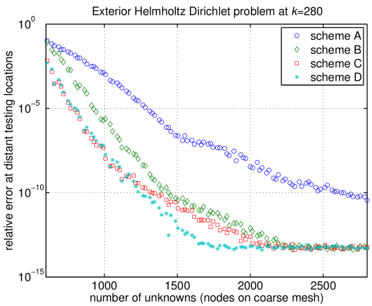
Figure 1: Far field tests of the schemes of Section 8.

We choose underlying Gauss–Legendre quadrature with $n_{\rm pt}=16$ and use the GMRES iterative solver [18] for the linear systems. The GMRES implementation involves a low-threshold stagnation avoiding technique [7, Section 8] applicable to systems coming from discretizations of Fredholm second kind integral equations. The stopping criterion threshold in the (estimated) relative residual is set to machine epsilon ($\epsilon_{\rm mach}$).

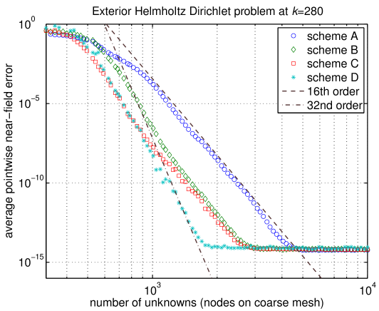
Figure 2: Near field tests of the schemes of Section 8.

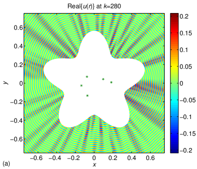
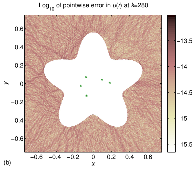
Figure 3: Field and error at 347650 near-field points computed with scheme C and 3904 unknowns on $\gamma$. The sources $r_{{\rm p}i}$ of (53) that generate the boundary conditions are shown as green stars. (a) Real part of $u(r)$. (b) $\log_{10}$ of pointwise error in $u(r)$ normalized with the largest value of $|u(r)|$ in $E$.

Two test series are run. The first series measures the maximum relative pointwise error at nine distant “testing locations” [6]

$$r_{{\rm t}i}=1.25(\cos(2\pi(i-1)/9),\sin(2\pi(i-1)/9))\,,\quad i=1,\ldots,9\,.$$ (54)

The second series measures the average pointwise error, normalized with the largest value of $|u(r)|$, in a near-field zone. This zone is taken as the intersection of $E$ and the square $x,y\in[-0.75,0.75]$, where a Cartesian grid of $200\times 200$ field points $r$ is created. Points in $D$ are then excluded, leaving a number of 28,460 points where $u(r)$ is evaluated. Test results for the far field are presented in Figure 1 and for the near field in Figure 2.

Figure 1, where the $x$-axis has linear scaling as to facilitate comparison with Figure 4(c) of [6], shows that fine grid resolution of $M(r,r^{\prime})$ for $r^{\prime}$ close to $r$ (scheme B) substantially improves on pure coarse grid resolution (scheme A). The number of unknowns needed to resolve $\rho(r)$, for a given accuracy in the far field $u(r)$, is roughly cut in half. The benefit of using unit speed parameterization (scheme C) is clearly visible too. Extended interpolation (scheme D) is only worthwhile when the highest achievable accuracy is of interest. A comparison between our scheme B and the 10th order accurate “Modified Gaussian” scheme of [6] reveals that scheme B converges faster, as expected. For example, with 1600 discretization points on $\gamma$ the gain in accuracy is around three digits. The achievable accuracy of those of our schemes that have saturated is on par with that of Kress’ global explicit-split scheme [15], which is the most accurate of the schemes tested in [6] and which also exhibits a more rapid convergence than any of our schemes in this example.

The results of the near field tests in Figure 2 are similar to those of the far field tests. The 16th order convergence of scheme A is apparent thanks to the logarithmic scaling of the $x$-axis. Schemes B and C also exhibit asymptotic 16th order convergence while scheme D converges more rapidly and with no evident asymptotics visible. Further experiments (not shown) indicate that the choice $n_{\rm s}=4$ in scheme D is optimal in the sense that larger $n_{\rm s}$ do not improve the convergence.

The actual field $u(r)$ and an example of a near-field error plot produced by scheme C are shown in Figure 3(a) and 3(b). A Cartesian grid of $700\times 700$ field points is used to produce these images. One can see, in Figure 3(b), that the field error is uniformly small all the way up to the boundary $\gamma$ although the convergence close to concave parts of $\gamma$ is, in fact, somewhat delayed compared to that in the remainder of $E$. The field point that happens to lie closest to $\gamma$ in this example is only separated from $\gamma$ by a distance of $3\cdot 10^{-6}$. Further tests (not shown) indicate that our product integration scheme can evaluate $u(r)$ at $r\in E$ arbitrarily close to $\gamma$ without the error deteriorating except for when $r$ lies extremely close to an endpoint of a panel. Then cancellation occurs in the quantities p(1) and p1 of Appendix B. In this case a procedure involving temporary panels mergers and splits can restore the accuracy [7, Section 5.5].

The achievable pointwise precision for $u(r)$ ranges between 13 and 15 digits in all our resolved examples. This is comparable to the precision obtained by Barnett in a similar example, exterior to a domain 12 wavelengths in diameter, using Kress’ global explicit-split scheme with a QBX post-processor [2, Section 4.1]. Given that the condition numbers of the main system matrices ${\bf I}+{\bf M}_{\gamma}$ in our schemes are very low, less than eight for $k=280$, one could speculate that it is possible to construct even more accurate schemes.

We end with some comments on the convergence of the GMRES iterative solver and on the influence of the coupling parameter $\eta$, discussed in Remark 2.1. With $\eta=k/2$ (our preferred choice) and the stopping criterion threshold set to $\epsilon_{\rm mach}$, GMRES converges in 51 iterations for all schemes and most resolutions in Figures 1 and 2. Severely underresolved systems require more iterations, though. With the choice $\eta=k$, made in [6, Equation (7.7)], the typical number of iterations required for full convergence rises to 60. The choice $\eta=-k$, made in the work on direct solvers for 3D scattering problems [4, Equation (2.3)], gives a particular slow convergence in GMRES – as also noted in [4, Remark 6.1]. A number of 373 iterations is needed in our experiments. In order to compare our GMRES convergence results to those of [6, Table 2], we increase the stopping criterion threshold to $10^{-12}$ and lower the wavenumber to $k=2.8$. Then 13 iterations are needed. This is marginally better than the 14 iterations reported for all competitive schemes in [6, Table 2].

10 Discussion

Initially, the thought of implementing an explicit kernel-split panel-based Nyström discretization scheme for planar Helmholtz boundary value problems may seem daunting because of the hefty series representations of Hankel functions that one can encounter when searching the special functions literature for information about the kernel singularities of the single- and double layer operators $S_{k}$ and $K_{k}$. But, when the dust has settled, the kernel splits can be written out in amazingly simple forms which, essentially, only involve functions that need to be evaluated also in split-free schemes. With access to efficient product integration techniques for logarithmic- and Cauchy-type singular kernels, the implementation is very straightforward.

The present paper shows that, for planar problems, the explicit kernel-split philosophy with quadratures computed on the fly offers rapid and stable convergence for linear systems as well as for far field and near field solutions. It, further, allows for the construction of schemes where mixes of discretizations on coarse and fine meshes enhance the performance.

In three dimensions the situation is more involved. For one thing, product integration for singular kernels is problematic. While it is possible to carry the techniques of the present work over to axisymmetric Helmholtz problems (a modification of scheme B is used in [11]), it is quite likely that schemes relying on adaptive and precomputed quadratures are better suited to solving fully three dimensional problems [4].

Acknowledgements. Johan Helsing wishes to thank the Banff International Research Station, Alberta, Canada (BIRS) and its staff for providing a creative atmosphere at the workshop “Integral Equations Methods: Fast Algorithms and Applications” in December 2013 where parts of this work were finalized. The work was supported by the Swedish Research Council under grant 621-2011-5516.

Appendix A: code for $\mathfrak{W}_{\rm L}$

The following Matlab function returns the $n_{\rm pt}\times n_{\rm pt}$ matrix $\mathfrak{W}_{\rm L}$, needed for the construction of the product integration weight corrections $w_{{\rm L}j}^{\rm corr}(r_{i})$ of (31):

  function WfrakL=WfrakLinit(trans,scale,tfrak,npt)
  A=fliplr(vander(tfrak));
  tt=trans+scale*tfrak;
  Q=zeros(npt);
  p=zeros(1,npt+1);
  c=(1-(-1).^(1:npt))./(1:npt);
  for m=1:npt
    p(1)=log(abs((1-tt(m))/(1+tt(m))));
    p1=log(abs(1-tt(m)^2));
    for k=1:npt
      p(k+1)=tt(m)*p(k)+c(k);
    end
    Q(m,1:2:npt-1)=p1-p(2:2:npt);
    Q(m,2:2:npt)=p(1)-p(3:2:npt+1);
    Q(m,:)=Q(m,:)./(1:npt);
  end
  WfrakL=Q/A;

The choice of input arguments trans=0 and scale=1 gives $\mathfrak{W}_{\rm L}$ for $r_{i}$ and $r_{j}$ on the same quadrature panel $\gamma_{p}$. The choice trans=$\pm$2 and scale=1 gives $\mathfrak{W}_{\rm L}$ for $r_{i}$ on a neighboring panel $\gamma_{p\pm 1}$, assuming it is equal in parameter length. The input argument tfrak is a column vector whose entries contain the canonical nodes $\mathfrak{t}_{i}$, $i=1,\ldots,n_{\rm pt}$, and npt corresponds to $n_{\rm pt}$.

Note that special-purpose quadrature only must be activated when $r_{i}$ and $r_{j}$ are close to each other, see Section 6.3, and that no closeness check is included in ${\tt WfrakLinit}$. Furthermore, a marginal improvement in accuracy can result from running the recursion for p backwards in certain situations, see [7, Section 6].

Appendix B: code for $w_{{\rm L}j}^{\rm corr}(r)$ and $w_{{\rm C}j}^{\rm cmp}(r)$

The following Matlab function returns the weight corrections $w_{{\rm L}j}^{\rm corr}(r)$ and the compensation weights $w_{{\rm C}j}^{\rm cmp}(r)$, $j=1,\ldots,n_{\rm pt}$, needed in (29) and (33) when $r\in E$:

  function [wcorrL,wcmpC]=wLCinit(ra,rb,r,rj,nuj,rpwj,npt)
  dr=(rb-ra)/2;
  rtr=(r-(rb+ra)/2)/dr;
  rjtr=(rj-(rb+ra)/2)/dr;
  A=fliplr(vander(rjtr)).’;
  p=zeros(npt+1,1);
  q=zeros(npt,1);
  c=(1-(-1).^(1:npt))./(1:npt);
  p(1)=log(1-rtr)-log(-1-rtr);
  p1=log(1-rtr)+log(-1-rtr);
  if imag(rtr)>0 && abs(real(rtr))<1
    p(1)=p(1)-2i*pi;
    p1=p1+2i*pi;
  end
  for k=1:npt
    p(k+1)=rtr*p(k)+c(k);
  end
  q(1:2:npt-1)=p1-p(2:2:npt);
  q(2:2:npt)=p(1)-p(3:2:npt+1);
  q=q./(1:npt)’;
  wcorrL=imag(A\q*dr.*conj(nuj))./abs(rpwj)-log(abs((rj-r)/dr));
  wcmpC=imag(A\p(1:npt)-rpwj./(rj-r));

This function relies on complex arithmetic and takes, as input, points and vectors in $\mathbb{R}^{2}$ represented as points in $\mathbb{C}$. Otherwise the notation follows Section 6: input parameters ra and rb correspond to $r(t_{a})$ and $r(t_{b})$; r is the target point $r\in E$; and rj, nuj, and rpwj are column vector whose entries contain the points $r_{j}$, the exterior unit normals $\nu$ at $r_{j}$, and the weighted velocity function $\dot{r}_{j}w_{j}$, $j=1,\ldots,n_{\rm pt}$.

References

- [1] K.E. Atkinson, The numerical Solution of Integral Equations of the Second Kind, Cambridge University Press, Cambridge, 1997.
- [2] A.H. Barnett, ‘Evaluation of layer potentials close to the boundary for Laplace and Helmholtz problems on analytic planar domains’, SIAM J. Sci. Comput., 36, A427–A451 (2014).
- [3] T. Betcke, S.N. Chandler-Wilde, I.G. Graham, S. Langdon, M. Lindner, ‘Condition number estimates for combined potential integral operators in acoustics and their boundary element discretisation’, Numer. Meth. Part. D. E., 27, 31–69 (2011).
- [4] J. Bremer, A. Gillman, P.G. Martinsson, ‘A high-order accurate accelerated direct solver for acoustic scattering from surfaces’, arXiv:1308.6643v1 [math.NA] (2013).
- [5] D. Colton and R.Kress, Inverse Acoustic and Electromagnetic Scattering Theory, Springer, Berlin, 1998.
- [6] S. Hao, A.H. Barnett, P.G. Martinsson, and P. Young ‘High-order accurate methods for Nyström discretization of integral equations on smooth curves in the plane’, Adv. Comput. Math., 40, 245–272 (2014).
- [7] J. Helsing and R. Ojala, ‘On the evaluation of layer potentials close to their sources’, J. Comput. Phys., 227, 2899–2921 (2008).
- [8] J. Helsing, ‘Integral equation methods for elliptic problems with boundary conditions of mixed type’, J. Comput. Phys., 228, 8892–8907 (2009).
- [9] J. Helsing, ‘Solving integral equations on piecewise smooth boundaries using the RCIP method: a tutorial’, Abstr. Appl. Anal., 2013, article ID 938167 (2013).
- [10] J. Helsing and A. Karlsson, ‘An accurate boundary value problem solver applied to scattering from cylinders with corners’, IEEE Trans. Antennas Propag., 61, 3693–3700 (2013).
- [11] J. Helsing and A. Karlsson, ‘An explicit kernel-split panel-based Nyström scheme for integral equations on axially symmetric surfaces’, J. Comput. Phys., 272, 686–703 (2014).
- [12] K.L. Ho and L. Greengard, ‘A fast direct solver for structured linear systems by recursive skeletonization’, SIAM J. Sci. Comput., 34, A2507–A2532 (2012).
- [13] A. Klöckner, A. Barnett, L. Greengard, and M. O’Neil, ‘Quadrature by expansion: A new method for the evaluation of layer potentials’, J. Comput. Phys., 252, 332–349 (2013).
- [14] P. Kolm and V. Rokhlin, ‘Numerical quadratures for singular and hypersingular integrals’, Comput. Math. Appl., 41, 327–352 (2001).
- [15] R. Kress, ‘Boundary integral equations in time-harmonic acoustic scattering’, Mathl Comput. Modelling, 15, 229–243 (1991).
- [16] R. Kress, Linear Integral equations, 2nd ed., Springer, New York, 1999.
- [17] M. Mitrea, ‘Boundary value problems and Hardy spaces associated to the Helmholtz equation in Lipschitz domains’, J. Math. Anal. Appl., 202, 819–842 (1996).
- [18] Y. Saad and M.H. Schultz, ‘GMRES: A generalized minimal residual algorithm for solving nonsymmetric linear systems’, SIAM J. Sci. Stat. Comp., 7, 856–869 (1986).