Physical aspects of heterogeneities in multi-component lipid membranes

Abstract

Ever since the raft model for biomembranes has been proposed, the traditional view of biomembranes based on the fluid-mosaic model has been altered. In the raft model, dynamical heterogeneities in multi-component lipid bilayers play an essential role. Focusing on the lateral phase separation of biomembranes and vesicles, we review some of the most relevant research conducted over the last decade. We mainly refer to those experimental works that are based on physical chemistry approach, and to theoretical explanations given in terms of soft matter physics. In the first part, we describe the phase behavior and the conformation of multi-component lipid bilayers. After formulating the hydrodynamics of fluid membranes in presence of the surrounding solvent, we discuss the domain growth-law and decay rate of concentration fluctuations. Finally, we review several attempts to describe membrane rafts as two-dimensional microemulsion.

1 Introduction

Biomembranes, which delimit the boundaries of biological cells, as well as the perimeter of intra-cellular organelles, play a vital role in maintaining and regulating cellular functions [1]. For example, mitochondria and chloroplast are examples of specific cellular organelles that use concentration gradient of ions across their membrane to supply energy that is indispensable to biological activities.

The main building blocks of biomembranes are a variety of phospholipids, glycosphingolipids and cholesterol. Phospholipids and glycolipids are amphiphilic molecules consisting of two moieties: a hydrophilic head group and, typically, two hydrophobic hydrocarbon chains. When lipid molecules are dissolved in water, they spontaneously form a bilayer membrane, where the hydrocarbon tails of the two leaflets face each other and point away from the water phase, in order to avoid direct contact between the hydrophobic hydrocarbon chains and water. In addition, various types of proteins are embedded within the biomembrane, and among other roles, they mediate the transport of substances between the inside and outside of the cell.

At physiological temperatures, biomembranes are fluid. This guarantees that both lipids and proteins can freely diffuse laterally within the membrane plane. A dynamical picture of biomembranes was provided by Singer and Nicolson in 1972, and their model was named the "fluid mosaic model" [2]. Although this model became a widely accepted standard model of biomembranes, the so-called "raft model" proposed by Simons and Ikonen [3] in 1997 initiated a substantial debate in the community regarding the nature of structural heterogeneities of biomembranes and their implied function.

According to the fluid mosaic model, various lipids and proteins are considered to be uniformly distributed within the membrane plane, while the raft model asserts the existence of nanoscale domains consisting of cholesterol and specific phospholipids such as sphingolipid. These lipid domains together with membrane proteins are expected to act as relay stations for signaling transfer factor, and to be involved in controlling quite a number of biological processes.

Based on the accumulated experimental results, a definition of lipid rafts has been suggested in an international conference held in 2006 [4]:

Membrane rafts are small (10–200 nm), heterogeneous, highly dynamic, sterol and sphingolipid-enriched domains that compartmentalize cellular processes. Small rafts can sometimes be stabilized to form larger platforms through protein-protein and protein-lipid interactions.

However, even today, there are still a large number of unresolved questions with regard to the origin and actual nature of membrane rafts in vivo and in vitro [5]. One of the reasons why the scientific community has been unable to settle the issue concerning the raft hypothesis is due to a lack of direct visualization of rafts in bio-membranes. Nevertheless, the raft hypothesis has largely stimulated the interest of physicists and physical chemists, leading to many studies on heterogeneities and phase separation of model lipid membranes.

In this article, we review the physical phenomenon that is induced by phase separation in multi-component lipid membranes, and describe related experimental and theoretical studies. However, it should be noted with care that exactly how the observed structures in model bilayers are related to lipid rafts in biomembranes is not completely understood at present. Nevertheless, the real picture of lipid rafts may become more evident as we explore physical mechanisms and concepts such as diffusion, phase separation and critical phenomena, because those mechanisms are well-defined and can be quantitatively measured and investigated in model systems.

The outline of this article is as follow. In the next section, we explain some known facts concerning lateral phase separation in multi-component membranes and review several physical models that describe it. In Sec. 3, we discuss the coupling between the lateral phase separation with membrane deformation and vesicle shape. Section 4 deals with hydrodynamics of fluid membranes embedded in a surrounding solvent. Based on hydrodynamic arguments, we review the dynamics of lateral phase separation in Sec. 5, particularly focusing on domain growth-law below the transition temperature. In Sec. 6, we summarize several results on the dynamics of concentration fluctuations above the transition temperature, and Sec. 7 is concerned with several recent attempts to view membrane rafts as two-dimensional microemulsion. Finally, an outlook is provided in the last section.

2 Lateral phase separation in multi-component membranes

2.1 Structural phase-transition of lipid bilayers

Lipids, which are the building blocks of biomembranes, include phospholipids, glycosphingolipids, and cholesterol. Typical examples of phospholipids are phosphatidylcholine (PC), phosphatidylserine (PS), and sphingomyelin (SM). Below, we shall divide lipid molecules into two categories: "saturated lipids" which do not contain any unsaturated bond in their hydrocarbon chains, and "unsaturated lipids" which have at least one unsaturated bond. Although cholesterol is also a lipid, hereafter we shall refer only to phospholipids or glycosphingolipids as "lipids" and cholesterol will retain its name.

It is known that by changing temperature, single-component lipid bilayers will undergo a structural phase transition that reflects a change in the orientational order of the lipid hydrocarbon chains [6]. At high temperatures, lipid bilayers are in a "liquid-crystalline phase", whereas at low temperatures they are in a "gel phase", in which the lipid molecules hardly diffuse. Prior to the lipid raft hypothesis, the phase behavior of bilayers consisting of two types of lipids characterized by different transition temperatures has been investigated using various experimental methods [6]. Since saturated lipids typically have higher phase-transition temperature than unsaturated ones, a region of two-phase coexistence appears between the liquid-crystalline and gel phases over a certain temperature range.

Cholesterol, on the other hand, is known to exhibit a dual effect in lipid bilayers [7]. In the liquid-crystalline phase cholesterol promotes the packing of hydrocarbon chains, while it disrupts the chain ordering in the gel phase. In binary mixtures of lipid and cholesterol, a mixed phase called the "liquid-ordered phase" (L_o-phase) appears when cholesterol concentration is high enough. In this phase, even though the lipid hydrocarbon chains are relatively ordered, the membrane maintains its fluidity. For intermediate cholesterol concentrations, membranes undergo a liquid-liquid phase separation between the L_o-phase and a lipid-rich phase called the "liquid-disordered phase" (L_d-phase). The latter phase is identical to the previously introduced "liquid-crystalline phase", and the lipid hydrocarbon chains in this phase are less ordered as compared to the L_o-phase. Since the minority phase forms domains as a result of phase separation, these domains have been studied in hope to shed light on membrane rafts with whom they probably share some similarities.

2.2 Three-component lipid mixtures

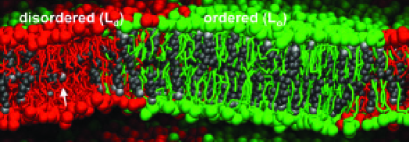
Figure 1: Coarse-grained molecular dynamics simulation of a three-component lipid bilayer membrane showing lateral phase separation. Green molecules are saturated lipids, red molecules are unsaturated lipids, and black molecules are cholesterol. The shown membrane is in a two-phase coexisting region between the L_o-phase (right) and the L_d-phase (left). The white arrow points to a cholesterol oriented in between the monolayer leaflets. Adapted from Ref. [12].

Dietrich et al. [8] were the first to visualize liquid domains in three-component lipid bilayers. Using fluorescence microscope, they observed phase-separated patterns in giant vesicles composed of unsaturated lipid, saturated lipid, and cholesterol. They demonstrated that the liquid-liquid phase separation indeed occurs because the L_o-phase rich in saturated lipid and cholesterol form circular two-dimensional (2d) liquid domains. Following this work, several other studies have been conducted [9, 10, 11] elucidating the phase behavior of various combinations of three-component mixtures (unsaturated lipid/saturated lipid/ cholesterol) as a function of temperature and composition. We note that a typical and well-studied three-component mixture is that of DOPC/DPPC/ cholesterol. In Fig. 1, we show a visualization obtained by coarse-grained molecular dynamics simulation [12] of a three-component lipid bilayer membrane exhibiting a lateral phase separation between L_o and L_d phases.

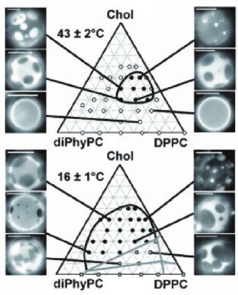
Figure 2: Fluorescence microscope images and ternary phase diagrams of giant vesicles composed of diPhyPC/DPPC/ cholesterol at 43 ^∘ C (top) and 16 ^∘ C (bottom). Dark circular domains in the side images are rich in DPPC and cholesterol. Open circles reside in the one-phase region of the phase diagrams, filled circles correspond to the two-phase coexisting region between the L_o-phase and the L_d-phase (liquid-liquid phase separation), and the gray squares indicate the gel phase. The scale bar corresponds to 20 $\mu$m. Adapted from Ref. [13].

For our later discussion, we show in Fig. 2 the experimentally obtained [13] ternary phase diagram of diPhyPC/DPPC/ cholesterol for two different temperatures: 43 ^∘C (top) and 16 ^∘C (bottom). Fluorescence microscope images of vesicles are also shown for different compositions. In these images, the white regions are rich in diPhyPC, while the dark ones are rich in DPPC and cholesterol. The open circles in the ternary phase diagram correspond to one-phase region (homogeneous phase), the filled circles to the two-phase coexisting region between the L_o-phase and the L_d-phase, and the gray squares indicate the gel phase. Interestingly, the two-phase coexistence region forms a closed loop at the higher temperature (43 ^∘C). At the lower temperature (16 ^∘C), two-phase coexistence region can be seen between the L_d-phase and the gel phase, below the triangular coexistence region of the three phases.

2.3 Theoretical models for lipid mixtures

There have been several theoretical attempts to predict and reproduce the phase behavior of multi-component lipid membranes. The membrane structural phase transition is generally first order, and is analogous to the nematic-isotropic transition in liquid crystals. Hence, the structural phase-transition of each type of lipid can be described by the Landau–de Gennes free-energy [14]. A model for biomembranes consisting of two types of lipids having different structural phase-transition temperature was proposed by Komura et al. [15, 16]. The phase-transition temperature of the binary lipid membrane was assumed to be a linear interpolation between the transition temperatures of the two pure components, and the model has been successful in explaining general phase behavior of various combinations of binary lipid mixtures.

As for lipid and cholesterol binary mixtures, by focusing on the dual effects of cholesterol as mentioned above, Ipsen et al. [7] proposed a microscopic model, while Komura et al. [15] developed a phenomenological model. It should be noted, however, that role of cholesterol is not yet fully understood.

Next, we review models addressing the phase behavior of three-component membranes in which cholesterol is added to a binary lipid mixture. For example, by using a self-consistent molecular model for cholesterol and lipids, Elliot et al. [17] calculated the phase diagram of ternary mixtures. Several phenomenological models have been also proposed [18, 19], among them, we briefly explain the model proposed by Putzel et al. [18]. In that work the area fraction (related to the relative concentration) of unsaturated lipid, saturated lipid, and cholesterol is denoted by $\phi_{\rm u}$, $\phi_{\rm s}$, and $\phi_{\rm c}$, respectively, and satisfies the incompressibility condition $\phi_{\rm u}+\phi_{\rm s}+\phi_{\rm c}=1$. In addition, a parameter $\delta$ is associated with the saturated lipids and characterizes the degree of orientational order of their hydrocarbon chains; the larger the value of $\delta$, the more orientational order of the hydrocarbon chains. The free-energy density $f_{\rm\ell}$ of the liquid phase was given by [18]

$$f_{\rm\ell} =J_{\rm ss}\phi_{\rm s}^{2}(\delta-1)^{2}+J_{\rm us}\phi_{\rm u}\phi_{\rm s}\delta-J_{\rm cs}\phi_{\rm c}\phi_{\rm s}\delta(1-\delta),$$

$$+k_{\rm B}T(\phi_{\rm u}\ln\phi_{\rm u}+\phi_{\rm s}\ln\phi_{\rm s}+\phi_{\rm c}\ln\phi_{\rm c})$$ (1)

where $k_{\rm B}$ is the Boltzmann constant, $T$ the temperature, and $J_{\rm ss}$, $J_{\rm us}$, $J_{\rm cs}$ are all positive interaction parameters. The $J_{\rm ss}$ term represents the interaction between two saturated lipids and depends on the orientational order $\delta$. In a similar way, the $J_{\rm us}$ and $J_{\rm cs}$ terms correspond to unsaturated-saturated lipids and cholesterol-saturated lipid interactions, respectively. The last three terms account for the ideal entropy of mixing.

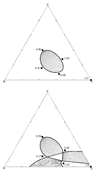
Figure 3: Ternary phase diagram of saturated lipid, unsaturated lipid and cholesterol, as obtained from the free energy in Eq. (1). The triangular corners "u", "s", and "c" represent unsaturated lipid, saturated lipid, and cholesterol, respectively. The top phase diagram corresponds to higher temperatures, while the bottom one to lower temperatures. The solid lines denote coexistence curves, thin lines are tie lines, and the numbers are the values of the $\delta$ parameter representing the orientational order of the saturated lipids. Adapted from Ref. [18].

The $J_{\rm us}$ term indicates that the effective repulsive interaction between unsaturated and saturated lipids becomes stronger when the orientational order $\delta$ increases. On the other hand, the negative term, proportional to ${-}J_{\rm cs}\delta$, expresses the tendency of cholesterol to increase the chain order $\delta$ of saturated lipids. Since the total repulsive interaction between unsaturated and saturated lipids is more enhanced according to this combined effect of cholesterol, the two lipids tend to segregate when cholesterol is present. The phase diagram, obtained by minimizing the above free-energy, is presented in Fig. 3 (top), and qualitatively reproduces the experimental closed-loop diagram, as shown in Fig. 2 (top). Moreover, by considering the free energy of the gel phase at lower temperatures, the theoretical phase diagram Fig. 3 (bottom) qualitatively reproduces the experimental one, shown in Fig. 2 (bottom).

2.4 Coupling between the two membrane leaflets

In biomembranes of living cells, the two monolayers (leaflets) have in general different composition, with a unique asymmetry between the inner and outer leaflets [20]. This asymmetry is essential to the biological function of the cell and is maintained by active processes such as lipid "flip-flop". Furthermore, the two leaflets are not independent, but rather interact strongly with each other due to various physical and chemical mechanisms [21, 22].

One of the interesting consequences is that a phase separation occurring in one leaflet can affect the other leaflet in a complex way. Using the Montal–Müller technique, Collins et al. [23] addressed the leaflet asymmetry within an artificially constructed bilayer, which biomimics the in-vivo situation. Two lipid monolayers have been combined, after each of them being individually prepared as a Langmuir monolayer with its own lipid composition, and the phase behavior was investigated for such coupled asymmetric monolayers. When one monolayer having a composition that does not exhibit phase separation was coupled with a second monolayer that was in its two-phase coexistence state, a phase separation was induced in the former monolayer. In addition, the experiment has shown strong positional correlation and domain registration between domains across the two membrane leaflets.

Inspired by the above experiment, a few phenomenological models have been proposed [24, 25] to describe the phase separation in such coupled leaflets. Several suggestions have been made about the possible physical origin of leaflet coupling, and they include van der Waals interactions, electrostatic interactions, or mutual interdigitation of hydrocarbon chains [22].

3 Phase separation and conformation changes in membranes

3.1 Domain-induced budding

Two-dimensional lipid bilayers can take various conformations in the three-dimensional (3d) embedded space. The observation that even vesicles consisting of a single component lipid exhibit a variety of complex shapes has been known for a long time. The most well-known model that describes the shapes of lipid membranes or vesicles is the "spontaneous curvature model" pioneered by Helfrich in the early 1970’s [26]. According to Helfrich model, a membrane is represented as a 2d curved surface of zero thickness, and its shape is governed by the following curvature elasticity free-energy

$$F_{\rm c}=\frac{\kappa}{2}\int{\rm d}A\,(C_{1}+C_{2}-2C_{0})^{2}+\bar{\kappa}\int{\rm d}A\,C_{1}C_{2}.$$ (2)

In the above equation, $C_{1}$ and $C_{2}$ are the two principle curvatures of the membrane surface related to the mean and Gaussian curvatures, $C=(C_{1}+C_{2})/2$ and $G=C_{1}C_{2}$, respectively, and the integration is performed over the entire surface area $A$ of the membrane. The coefficients $\kappa$ and $\bar{\kappa}$ are the bending and saddle-splay moduli, respectively, $C_{0}$ is the material-dependent spontaneous curvature, reflecting any potential asymmetry between the two sides of the membrane. For a vesicular shape, by minimizing Eq. (2) under the condition that both the total area $A$ and total inner volume $V$ are conserved, one can obtain a variety of vesicle shapes that are mechanically stable.

What happens to the membrane shape when the lateral phase separation takes place in a multi-component lipid bilayer? The line tension acting at the edge of the 2d domains due to the phase separation plays here an important role. Prior to any experimental works, Lipowsky [29] proposed the idea of domain-induced budding in multi-component membranes, to be reviewed next.

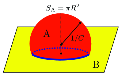
Figure 4: A bud (A-domain) forming a spherical cap of radius $1/C$ where $C$ is the curvature, embedded in a flat B-domain. The total area of the A-domain is $S_{\rm A}=\pi R^{2}$. The line tension $\sigma$ is acting along the boundary (blue line) between the A and B domains.

Let’s us consider a single 2d circular domain of radius $R$ embedded in a flat 2d membrane, as shown in Fig. 4. The domain is characterized by a line tension $\sigma$ that acts at the 1d edge (perimeter) of the domain. Budding of the domain is a process where the domain protrudes in the third dimension (perpendicular to the membrane plane). For simplicity, we assume that the budded domain shape is a spherical section of a sphere of radius $1/C$. The total energy of the budded domain is given by the sum of the curvature elasticity energy, Eq. (2), and the line energy that is proportional to the domain boundary length (the "neck"):

$$F_{\rm d}=2\pi\kappa\left[(RC-RC_{0})^{2}+(R/\ell)\sqrt{1-(RC/2)^{2}}\right],$$ (3)

where $\ell=\kappa/\sigma$ is called the "invagination length", and $RC$ is the dimensionless curvature.

The boundary values $RC=\pm 2$ correspond to the "complete budding", while $RC=0$ represents the 2d flat domain. When the spontaneous curvature is nonzero ($C_{0}\neq 0$), the symmetry between the two sides of the membrane is broken. If the value of $R/\ell$ is small enough, the minimization of total domain energy, Eq. (3), yields intermediate $RC$ values, $0<|RC|<2$. This situation for which the curvature elasticity energy and the line energy balances each other is called "incomplete budding".

3.2 Phase separation in multi-component vesicles

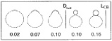
Figure 5: Equilibrium shapes of vesicles consisting of two domains (A-domain: solid line, B-domain: dashed line). All these shapes are axisymmetric. The numbers indicate the areal fraction of the A-domain, $\phi_{\rm A}$. A discontinuous budding transition occurs at D_bud, while a singular limit shape with closed neck occurs at L_CB. Adapted from Ref. [31].

In Lipowsky’s model, the embedding matrix surrounding the domain was assumed to be infinitely large and flat. Later, domain-induced budding for closed-shaped and curved vesicles was investigated in great detail by Jülicher and Lipowsky [30, 31]. Assuming that a vesicle is composed of two coexisting domains of type A and B, Jülicher and Lipowsky considered the curvature elasticity energy, Eq. (2), for the two domains, together with the line tension $\sigma$ acting at the domain boundary. The total free energy was minimized under the constraint of constant area and volume of the vesicle. The obtained equilibrium vesicle shape [31] as function of the $\phi_{\rm A}$, the area fraction of the A-domain (represented by a solid line) is shown in Fig. 5. For $\phi_{\rm A}=0.1$, a discontinuous transition from incomplete budding to complete budding takes place. When $\phi_{\rm A}=0.16$, each domain forms a sphere on its own, and the neck connecting the two spheres disappears.

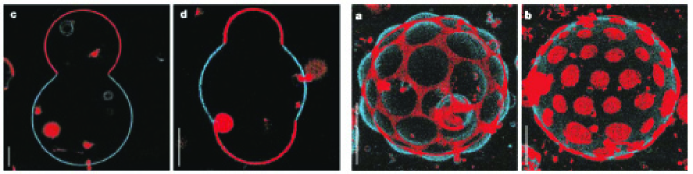
Figure 6: Two-photon microscopy images of giant vesicles consisting of DOPC/SM/ cholesterol. Blue and red domains correspond to the L_o-phase and the L_d-phase, respectively. In the left two pictures, different phases have different curvatures. In the right two pictures, finite-sized domains are ordered in a periodical fashion. The scale bar corresponds to 5 $\mu$m. Adapted from Ref. [32].

Baumgart et al. [32] considered experimentally the interplay between the shape and lateral phase separation in vesicles. We show the results in Fig. 6 (left), for vesicles composed of DOPC/SM/ cholesterol. These results demonstrate that each domain is characterized by a distinct curvature, and multi-domain vesicles form spontaneously complex structures. The analysis of these vesicle shapes showed that the observed morphology can be explained in terms of the model of Jülicher and Lipowsky [33], although some of the experimental reported shapes are probably only metastable.

Moreover, Baumgart et al. [32] sometimes found vesicles that do not undergo macroscopic phase separation, but rather form 2d ordered patterns of finite-size domains as is reproduced in Fig. 6 (right). Such patterns are an indication of the so-called micro-phase separation — a well-studied phenomena characterizing equilibrium structures of block copolymers and surfactant solutions [34]. Although it still remains unclear under what conditions micro-phase separation can be obtained in bilayers, some recent studies [35, 36] have reported that micro-phase separation can be induced by controlling the composition of membranes composed of four-component lipid mixtures. The appearance of such micro-phase separated structures in membranes or vesicles has been explained in terms of the curvature instability mechanism [37, 38, 39, 40]. Several possible physical mechanisms, including the curvature instability that leads to micro-phase separations will be addressed separately in Sec. 7 below.

Yanagisawa et al. [41] found that when salt was added to multi-component vesicles in order to control the osmotic pressure difference, complex shape transformations took place followed by domain budding. Furthermore, multi-component membranes containing charged lipids have been also studied experimentally [42]. In general, phase separation is suppressed because it is energetically unfavorable to form charged domains [43].

4 Hydrodynamic effects in fluid membranes

4.1 Mobility tensor of fluid membranes

So far, we have regarded the equilibrium properties of multi-component membranes and vesicles. We proceed by reviewing the hydrodynamic properties of fluid membranes and discuss, in particular, the dynamics of their heterogeneities. In their pioneering work, Saffman and Delbrück considered a hydrodynamic model for biomembranes based on the fluid mosaic model [44, 45]. Their main purpose was to obtain the diffusion coefficient of a protein molecule embedded inside a fluid membrane. Since the lateral extent of the membrane surface is typically much larger than its thickness, it is justified to regard the membrane as a 2d fluid of zero thickness. However, if one employs the Stokes approximation in order to analyze the stationary motion of an isolated object embedded in an infinitely extended 2d fluid, we are faced with the so-called Stokes paradox [46], where the hydrodynamic equation does not have a solution. The Stokes paradox originates from the inability to conserve momentum within a 2d fluid.

On the other hand, because a fluid membrane is not an isolated 2d system but surrounded by a 3d solvent (water), the Stokes paradox can be avoided if the dissipation of the membrane momentum is included into the surrounding 3d solvent. The obtained diffusion coefficient is given below by Eq. (9), and has been extensively used in analyzing experimental data [6]. Hereafter, we consider a slightly more generalized situation and explain how to derive the hydrodynamic mobility tensor.

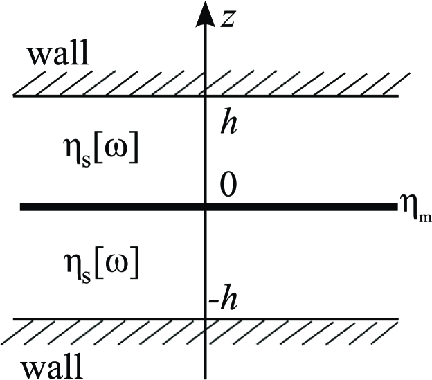
Figure 7: Generalized Saffman and Delbrück hydrodynamic model. Planar viscous membrane at $z=0$ of 2d viscosity $\eta_{\rm m}$ is sandwiched in between two solvents having the same 3d viscosity $\eta_{\rm s}$. Two impenetrable walls at $z=\pm h$ bound the upper and lower solvents. When the solvent is viscoelastic, its viscosity $\eta_{\rm s}[\omega]$ becomes frequency dependent.

Consider an infinitely extended 2d flat fluid membrane of 2d viscosity $\eta_{\rm m}$, as shown in Fig. 7 [47, 48], sandwiched between an upper and a lower 3d solvents of the same 3d viscosity $\eta_{\rm s}$. Note that the units of the 3d viscosity $\eta_{\rm s}$ and 2d viscosity $\eta_{\rm m}$ are different. Two solid walls are placed at distance $h$ from the membrane making the thickness of the solvents finite. This setup is motivated by many experiments that are performed on supported lipid bilayers placed on top of a solid substrate. The inplane velocity vector of the fluid membrane is denoted by ${\mathbf{v}}({\mathbf{r}})$ where ${\mathbf{r}}=(x,y)$ is a 2d position vector. Assuming that the incompressibility condition holds for the fluid membrane, we write its hydrodynamic equations as

$$\nabla\cdot{\mathbf{v}}=0,$$

$$\eta_{\rm m}\nabla^{2}{\mathbf{v}}-\nabla p+{\mathbf{f}}_{\rm s}+{\mathbf{F}}=0.$$ (4)

The second equation is the 2d Stokes equation, where $p$ is the lateral pressure, ${\mathbf{f}}_{\rm s}$ is the force exerted on the membrane by the surrounding solvent, and ${\mathbf{F}}$ is any external force acting on the membrane.

If we denote the upper and lower solvents with the superscripts $\pm$, the two solvent velocities ${\mathbf{v}}^{\pm}({\mathbf{r}},z)$ and pressures $p^{\pm}({\mathbf{r}},z)$ obey the following hydrodynamic equations, respectively

$$\widehat{\nabla}\cdot{\mathbf{v}}^{\pm}=0,$$

$$\eta_{\rm s}\widehat{\nabla}^{2}{\mathbf{v}}^{\pm}-\widehat{\nabla}p^{\pm}=0,$$ (5)

where $\widehat{\nabla}$ stands for the 3d differential operator (while for convenience $\nabla$ denotes the operator in 2d).

The boundary conditions at the membrane are non-slip leading to matching of the membrane and solvent velocities at the membrane plane, $z=0$. Furthermore, the solvent velocity vanishes at the $z=\pm h$ walls. With the use of the solvent stress tensor we can write

$${\bm{\sigma}}^{\pm}=-p^{\pm}{\mathbf{I}}+\eta_{\rm s}[\widehat{\nabla}{\mathbf{v}}^{\pm}+(\widehat{\nabla}{\mathbf{v}}^{\pm})^{\rm T}],$$ (6)

where the ’T’ superscript stands for the transpose operator, the force ${\mathbf{f}}_{\rm s}$ is given by the projection of $\hat{{\mathbf{e}}}_{z}\cdot({\bm{\sigma}}^{+}-{\bm{\sigma}}^{-})_{z=0}$ onto the membrane, $\hat{{\mathbf{e}}}_{z}$ is the unit vector in the $z$-direction. By solving the above coupled hydrodynamic equations in Fourier space with $\mathbf{k}=(k_{x},k_{y})$ being the 2d wavevector, the 2d mobility tensor ${G}_{ij}({\mathbf{k}})$ defined through ${v_{i}}({\mathbf{k}})=\sum_{j}{G}_{ij}({\mathbf{k}}){F}_{j}({\mathbf{k}})$ ($i,j=x,y$) can now be written as

$$G_{ij}({\mathbf{k}})=\frac{1}{\eta_{\rm m}[k^{2}+\nu k\coth(kh)]}\left(\delta_{ij}-\frac{k_{i}k_{j}}{k^{2}}\right),$$ (7)

where $\nu^{-1}=\eta_{\rm m}/2\eta_{\rm s}$ is the hydrodynamic screening length and $k=|{\mathbf{k}}|$. We note that the above membrane mobility tensor is analogous to the Oseen tensor for 3d fluids [46], and the presence of the surrounding solvent of finite thickness (solid walls at $z=\pm h$) is accounted for by the second term of the denominator in Eq. (7).

4.2 Coupling diffusion: free membrane case

Saffman and Delbrück considered the limiting case of $kh\gg 1$ in Eq. (7), for which the denominator can be approximated by $\eta_{\rm m}(k^{2}+\nu k)$. This situation is equal to the free membrane case because there is no dependence on the bounding walls and solvent thickness, $h$. We consider two point-particles (particle 1 and 2) separated by distance $r$ on the membrane, and discuss the longitudinal coupling diffusion coefficient $D_{\rm L}$ defined by $\langle\Delta x_{1}\Delta x_{2}\rangle_{r}=2D_{\rm L}(r)t$, where $\Delta x_{i}$ is the displacement of the $i$-th particle along the line connecting the two point-particles, and $t$ is time. By taking the inverse Fourier transform of the mobility tensor and using the Einstein relation, the coupling diffusion coefficient is obtained as [49, 50]

$$D_{\rm L}(r)=\frac{k_{\rm B}T}{4\pi\eta_{\rm m}}\left[\frac{\pi{\mathbf{H}}_{1}(\nu r)}{\nu r}-\frac{\pi Y_{1}(\nu r)}{\nu r}-\frac{2}{(\nu r)^{2}}\right],$$ (8)

where ${\mathbf{H}}_{1}(x)$ and $Y_{1}(x)$ are the Struve function and the Bessel function of the second kind, respectively.

There are two asymptotic limits of Eq. (8) depending on the value of $\nu r$. In the small separation limit, $\nu r\ll 1$,

$$D_{\rm L}(r)\approx\frac{k_{\rm B}T}{4\pi\eta_{\rm m}}\left[\ln\left(\frac{2}{\nu r}\right)-\gamma+\frac{1}{2}\right],$$ (9)

where $\gamma=0.5772\cdots$ is the Euler’s constant, whereas in the large separation limit, $\nu r\gg 1$

$$D_{\rm L}(r)\approx\frac{k_{\rm B}T}{2\pi\eta_{\rm m}\nu r}=\frac{k_{\rm B}T}{4\pi\eta_{\rm s}r}.$$ (10)

It is worth mentioning that the coupling diffusion coefficient $D_{\rm L}(r)$ between two point-particles separated by a distance $r$ corresponds to the self-diffusion coefficient of a single particle of size $r$ up to a prefactor of order unity.

The above results clearly demonstrate the hydrodynamic behavior of a 2d fluid membrane surrounded by 3d solvent. If the distance $r$ between two points on the membrane is sufficiently small compared with the hydrodynamic screening length $\nu^{-1}$, the diffusion coefficient is almost independent of $r$ (see Eq. (9)) [44, 45]. On the other hand, if $r$ is sufficiently large as compared with $\nu^{-1}$, $D_{\rm L}$ is inversely proportional to $r$ (see Eq. (10)), similar to the Stokes–Einstein relation for a 3d solid sphere [51].

In other words, Eq. (9) reflects the 2d nature of the fluid membrane, while Eq. (10) represents the 3d nature of the outer solvent. Since typical values of the hydrodynamic screening length $\nu^{-1}$ are in the sub-micron range, $\nu r\ll 1$ holds for usual membrane proteins whose size is in the nanometer rage. In contrast, it was experimentally demonstrated that the diffusion coefficient of micron-sized domains (much larger than a protein molecule), is inversely proportional to their size [52], in agreement with Eq. (10).

4.3 Coupling diffusion: confined membrane case

The other limit of $kh\ll 1$ in Eq. (7) corresponds to the confined membrane case, where the lipid bilayer is supported by a solid substrate (if there is only one wall). Evans and Sackmann were the first to consider such a case [53], and Seki and Komura and coworkers [54, 55, 56] applied it to membranes, whose momentum dissipates into the surrounding solvent with a characteristic decay rate.

For confined membranes the denominator in Eq. (7) can be approximated by $\eta_{\rm m}(k^{2}+\chi^{2})$ [57], where $\chi^{-1}=\sqrt{\nu^{-1}h}$ is the hydrodynamic screening length. The corresponding coupling diffusion coefficient can be obtained similarly to Eq. (8), and results in a logarithmic dependence when $\chi r\ll 1$. For $\chi r\gg 1$, however, $D_{\rm L}(r)\sim h/r^{2}$, which decays as $\sim 1/r^{2}$ rather than $\sim 1/r$ as in Eq. (10).

4.4 Effects of solvent viscoelasticity

In eukaryotic cells, the cytoplasm contains proteins, subcellular organelles as well as an actin meshwork forming the cell cytoskeleton [1]. In addition, the outside of the cell is composed of an extracellular matrix and/or hyaluronic acid gel that can be regarded as a polymer solution.

Komura et al. [58, 59] discussed the dynamics of biomembranes under the assumption that the surrounding solvent is viscoelastic, and we mention it here. The surrounding solvent was considered to obey the constitutive equation:

$${\bm{\sigma}}^{\pm}(t)=2\int_{-\infty}^{t}{\rm d}t^{\prime}\eta_{\rm s}(t-t^{\prime})\mathbf{D}^{\pm}(t^{\prime}),$$ (11)

where $\eta_{\rm s}(t)$ is the time-dependent solvent viscosity, and

$$\mathbf{D}^{\pm}=\frac{1}{2}[\widehat{\nabla}\mathbf{v}^{\pm}+(\widehat{\nabla}\mathbf{v}^{\pm})^{\rm T}],$$ (12)

is the rate-of-strain tensor.

By repeating the calculation along the lines done in Sec. 4.1, we obtain the mobility tensor $G_{ij}(\mathbf{k},\omega)$ that depends also on the frequency $\omega$. For simplicity, let us assume that the frequency dependence of the solvent viscosity obeys a power law: $\eta_{\rm s}(\omega)=G_{0}(i\omega)^{\beta-1}$ with $\beta<1$ because $\eta_{\rm s}(\omega)$ should vanish for $\omega\rightarrow\infty$. Notice that the purely viscous case is recovered for $\beta\rightarrow 1$. Using the fluctuation-dissipation theorem, it is possible to calculate the time-dependence of the two-particle correlation function $\langle\Delta x_{1}\Delta x_{2}\rangle_{r}$ from $G_{ij}(\mathbf{k},\omega)$. For large $r$, the correlation behaves asymptotically as $\langle\Delta x_{1}\Delta x_{2}\rangle_{r}\sim(k_{\rm B}T/G_{0}r)t^{\beta}$, which gives rise to anomalous diffusion since $\beta<1$ [58, 59]. Recently, anomalous diffusion of membrane proteins has been experimentally observed [60], but it should be equally noted that there are other mechanisms that may lead to such anomalous diffusion.

5 Dynamics of lateral phase separation

5.1 Experiments on domain growth-law

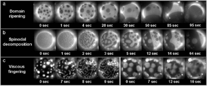
Figure 8: Time evolution of phase separation observed for ternary vesicles consisting of DOPC/DPPC/ cholesterol. (a) Domain growth (ripening) due to collision and coalescence when the ratio of the L_o-phase and L_d-phase is asymmetric. (b) Spinodal decomposition when the two phases are symmetric. (c) Viscous fingering when the two phases are highly asymmetric. Adapted from Ref. [10].

Investigations on phase separation in multi-component lipid bilayers initially focused on equilibrium properties such as phase behavior, as was explained in the previous sections. Later, substantial attention has been devoted to the dynamics of phase separation in membranes. For ternary mixtures of DOPC/DPPC/ cholesterol, Veatch et al. [10] reported several types of growth patterns depending on the relative membrane composition. When the area fraction between the L_o-phase and L_d-phase is asymmetric, as shown in Fig. 8(a), domain growth occurs. The process is dominated by the collision-coalescence mechanism rather than by the evaporation-condensation mechanism. When the area ratio between the two phases was almost symmetric, namely 1:1, spinodal decomposition was observed, as shown in Fig. 8(b).

When a dynamical scaling law holds, the average domain size $R$ increases according to a temporal power-law, $R(t)\sim t^{\alpha}$. Using fluorescence microscope, Saeki et al. [61] performed a quantitative measurement of the growth exponent $\alpha$ for vesicles consisting of DOPC/DPPC/ cholesterol, and reported the value $\alpha\approx 0.15$. Later, Yanagisawa et al. [62] conducted a similar experiment and found that there are two different types of domain growth that depend on system conditions (explained below). The first type is due to the collision-coalescence mechanism, with a growth exponent, $\alpha\approx 2/3$. For the second type, the domain growth was suppressed over a long period of time, although the domain size suddenly increased at the final stage of the phase separation.

Even though the conditions to distinguish between the two types of domain growth is not completely clear, the collision-coalescence mechanism is more dominant when the excess area of the vesicle is relatively small. When the excess area is large, budding of domains can take place, and the elastic interaction between the domains mediated by the membrane affects the phase separation dynamics. Finally, we note that recently Stanich et al. [63] performed a systematic experimental study on the growth exponent. They reported $\alpha=0.29\pm 0.05$ for asymmetric compositions, and $\alpha=0.31\pm 0.05$ for nearly symmetric compositions when the collision-coalescence mechanism was dominant.

5.2 Collision-coalescence mechanism of domain growth

Considerable theoretical interest has been devoted to the understanding of dynamics of phase separation in lipid membranes, and, in particular, several numerical studies were conducted [64, 65, 66] using computer simulations. Laradji et al. [67] used dissipative particle-dynamics method in order to simulate a two-component vesicle composed of coarse-grained lipid molecules [68, 69]. When the composition of the two lipids was asymmetric, the domain growth was driven by the collision-coalescence mechanism, and the growth exponent was found to be $\alpha\approx 0.3$. Moreover, it was reported that even budding of domains occurs when the excess area was large enough.

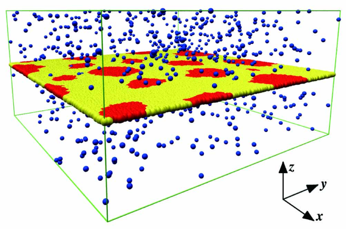
Figure 9: Binary fluid membrane with the surrounding solvent. The yellow (lipid A) and red (lipid B) particles represent the two components constituting the membrane, while the blue particles represent the solvent. For clarity, only a fraction of the solvent particles are shown.

Ramachandran et al. [70] performed a dissipative particle-dynamics simulation in order to investigate the hydrodynamic effects on the 2d membrane phase-separation when the membrane is placed in contact with a 3d solvent. As shown in Fig. 9, it was assumed that a flat fluid membrane is composed of A (yellow) and B (red) particles. The membrane is sandwiched by 3d solvent particles (blue), and its bilayer nature is neglected. The time evolution of the phase separation between the pure-2d membrane (no solvent) was compared with that of a quasi-2d one (with solvent particles). The result showed that the domain size in the quasi-2d case was smaller than for the pure-2d case over the same period of time. It offers an evidence that the phase separation in the quasi-2d membrane is suppressed. Even more quantitative analysis [70] reveals that the growth exponent for the pure-2d case is $\alpha=1/2$, while for quasi-2d case it is $\alpha=1/3$.

The various values of the growth exponent $\alpha$ can be explained as follows. The domain growth occurs through the collision-coalescence process driven by the Brownian motion of domains. If the domain size $R$ is the only relevant length scale, the scaling relation $R^{2}\sim Dt$ should hold, where $D$ is the domain diffusion coefficient, as discussed in the previous section. Since the hydrodynamic screening length $\nu^{-1}$ for the pure-2d membrane is considered to be infinitely large, $R$ is always smaller than $\nu^{-1}$, and the diffusion coefficient $D$ is almost constant, as shown in Eq. (9). Hence, we obtain $\alpha=1/2$ from the scaling $R\sim t^{1/2}$.

For the quasi-2d membrane, on the other hand, $\nu^{-1}$ is finite, and $R$ will become larger than $\nu^{-1}$ in the late stages of the phase separation. As a result, the 3d hydrodynamic interactions mediated by the solvent will become more important, and the diffusion coefficient behaves like $D\sim 1/R$, as given by Eq. (10). Thus, we obtain $R\sim t^{1/3}$ that explains why the growth exponent for the quasi-2d membrane is $\alpha=1/3$. We remark that this value is in accord with the recent experimental result by Stanich et al. [63].

5.3 Dynamics of concentration field

In order to describe the dynamics of phase separation in multi-component biomembranes using a continuous concentration field, one can employ the time-dependent Ginzburg–Landau (TDGL) model. The local area fractions (concentrations) of A and B lipids in binary membranes are denoted by $\phi_{\rm A}({\mathbf{r}},t)$ and $\phi_{\rm B}({\mathbf{r}},t)$, respectively. Since the incompressibility condition is given by $\phi_{\rm A}+\phi_{\rm B}=1$, it is enough to introduce an order parameter being the relative concentration: $\phi=\phi_{\rm A}-\phi_{\rm B}$. The Ginzburg–Landau free-energy that describes the phase separation of a binary membrane is given by

$$F_{\rm GL}[\phi]=\int{\rm d}{\mathbf{r}}\,\left[\frac{a}{2}\phi^{2}+\frac{1}{4}\phi^{4}+\frac{c}{2}(\nabla\phi)^{2}\right],$$ (13)

where $a\sim(T-T_{\rm c})$ is the reduced temperature and $c$ is related to the line tension $\sigma$.

The time evolution of the concentration field $\phi$, which is a conserved order parameter, can be described by the following dynamical equation [71]:

$$\frac{\partial\phi}{\partial t}+\nabla\cdot({\mathbf{v}}\phi)=L\nabla^{2}\frac{\delta F_{\rm GL}}{\delta\phi},$$ (14)

where $L$ is the transport coefficient. The membrane velocity ${\mathbf{v}}$ in the second term obeys the hydrodynamic equations described in Sec. 4. The velocity and concentration fields within the 2d membrane are coupled through the external force given by $\mathbf{F}=-\phi\nabla(\delta F_{\rm GL}/\delta\phi)$ in the 2d Stokes equation. The present model for quasi-2d fluid membranes is an extension of the so-called "Model H" introduced by Hohenberg and Halperin [72] to describe 3d fluids at criticality.

To study the dynamics of phase separation, this extended Model H was numerically solved by Camley et al. [73] and Fan et al. [74] in the presence of thermal noise. In addition to the previously mentioned collision-coalescence mechanism, domain coarsening in these simulations includes also the evaporation-condensation mechanism, driven by the line tension $\sigma$ between the domains. It results in a scaling relation of the domain growth given by $R\sim(L\sigma t)^{1/3}$ [73, 75]. Although the corresponding exponent $\alpha=1/3$ is independent of the spatial dimension, the growth exponent due to the collision-coalescence mechanism depends on the relative magnitude of $R$ and $\nu^{-1}$, as mentioned earlier.

When the average composition is asymmetric, various scaling regimes have been identified in the numerical simulations of the extended Model H [73]. However, the situation becomes somewhat more complicated when the average composition is symmetric. The simulations show that the coarsening of domains that are isotropic in their shape is slower than for anisotropic domains. This means that phase-separated patterns at different times are not characterized by a single length scale, and indicates a breakdown of the dynamical scaling law.

5.4 Non-equilibrium effects

It was suggested by several authors [76, 77] that raft formation in biomembranes is associated with the non-equilibrium natures of biomembranes, and potentially includes material exchange between the membrane and its surroundings. For example, Foret [78] proposed a time evolution equation for the concentration field $\phi$ by taking into account the lipid exchange with the surrounding:

$$\frac{\partial\phi}{\partial t}=L\nabla^{2}\frac{\delta F_{\rm GL}}{\delta\phi}-\Omega(\phi-\bar{\phi}).$$ (15)

In the above, $F_{\rm GL}[\phi]$ is the GL free-energy given by Eq. (13), $\Omega$ the lipid exchange rate, and $\bar{\phi}$ the spatial average value of $\phi$. It is interesting to note that as Eq. (15) is formally identical with the time evolution equation of block copolymers, it will lead to a micro-phase separation of domains, just as is the case in the block copolymer case [34]. Interested readers are referred to the work by Fan et al. [79] for other proposed origins of raft formation, such as partitioning effects of lipids, and the non-equilibrium transport of lipids, as well as to another model [80] suggesting cholesterol exchange (instead of lipid exchange) between the membrane and the outer surrounding solvent.

Recently dynamics of biomembranes mediated by chemical reactions has attracted some attentions. Hamada et al. [81] added photoresponsive amphiphile to a typical ternary lipid mixture, and showed that its conformation change can switch on a reversible lateral segregation of the membrane. They demonstrated that cis-isomerization induces lateral phase separation in membranes that are in their one-phase (homogeneous) region, while producing additional lateral domains in membranes that are in their two-phase coexisting regions.

6 Dynamics of concentration fluctuations

6.1 Critical phenomena in membranes

So far we have discussed domain formation that occurs at temperatures below the phase-separation temperature, and its induced structural changes in vesicles. Experimentally, concentration fluctuations above the critical temperature have been also observed. Veatch et al. [82] used Nuclear Magnetic Resonance (NMR) to measure the concentration fluctuations in DOPC/DPPC/ cholesterol mixtures, and extracted from the data the corresponding correlation-length.

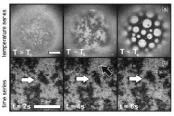
Figure 10: Fluorescence microscope images of giant vesicles composed of diPhyPC/DPPC/ cholesterol. The critical temperature is $T_{\rm c}=30.9$ ^∘C. (a) Concentration fluctuations ($T>T_{\rm c}$, one-phase region), criticality at $T\sim T_{\rm c}$, and domain growth ($T<T_{\rm c}$, two-phase coexistence region) are observed. (b) Time evolution of the concentration fluctuations for $T>T_{\rm c}$. The scale bar corresponds to 20 $\mu$m. Adapted from Ref. [85].

Another ternary mixture (diPhyPC/DPPC/ cholesterol) was used by Honerkamp-Smith et al. [83] to study vesicles whose membrane composition corresponds to critical phenomena. We reproduce their fluorescence microscope pictures of concentration fluctuations in Fig. 10. For these mixtures, the critical temperature is $T_{\rm c}=30.9$ ^∘C. Concentration fluctuations are observed for $T>T_{\rm c}$, while domain formation are observed for $T<T_{\rm c}$, (see Fig. 10(a)). From the experimental data, the critical exponent for the correlation length, $\xi\sim|T-T_{\rm c}|^{-1.2\pm 0.2}$, was extracted with the conclusion that the critical behavior of this ternary lipid mixture belongs to the universality class of the 2d Ising model.

Even more surprising, the 2d Ising critical behavior was also observed in biomembranes which were extracted from the basophil leukemic cells of a living rat [84]. These series of experiments proposed the possibility that heterogeneous structures in biomembranes under physiological conditions can be attributed to the critical concentration fluctuations. However, it is rather specific to systems that are in the close proximity of a critical point, and the application to biomembranes at physiological conditions is yet to be confirmed.

Recently, Honerkamp-Smith et al. [85] have elaborated also on the dynamics of concentration fluctuations in membranes. Figure 10(b) shows the time evolution of the concentration fluctuations and indicates that the structure of the large-scale fluctuations (white arrow in the figure) is sustained over few seconds, while the small-scale fluctuations (black arrow in the figure) disappear almost instantaneously. The relaxation time of the concentration fluctuations was measured in order to determine how it increases as the critical point is approached (critical slowing down). From the data it was suggested that a dynamic scaling law $\tau\sim\xi^{z}$ holds between the relaxation time $\tau$ and the correlation length $\xi$ with an exponent $z$. As the critical point is approached from above, the correlation length grew, and it was found that the apparent exponent crosses over from $z=2$ to $z=3$. Next we shall discuss this crossover behavior from a theoretical point of view.

6.2 Decay rate of concentration fluctuations

The dynamics of concentration fluctuations in biomembranes was modeled by Seki et al. [86]. They used the 2d hydrodynamic model that takes into account the momentum dissipation (i.e., confined membrane case) to calculate the intermediate time-dependent structure factor, $S({\mathbf{k}},t)$. This quantity is the spatial Fourier transform of the time-dependent correlation function $G_{\phi\phi}({\mathbf{r}},t)=\langle\delta\phi({\mathbf{r}},t)\delta\phi(0,0)\rangle$, where $\delta\phi({\mathbf{r}},t)$ is the concentration fluctuation. Solving the equations for the concentration and velocity fields it was found that the intermediate correlation function decays exponentially:

$$S({\mathbf{k}},t)=S({\mathbf{k}},0){\rm e}^{-\Gamma({\mathbf{k}})t}$$ (16)

with

$$\Gamma({\mathbf{k}})=k^{2}D_{\rm eff}({\mathbf{k}}),$$ (17)

where $\Gamma({\mathbf{k}})$ is the wavenumber-dependent decay rate (inverse of the relaxation time), from which the effective diffusion coefficient $D_{\rm eff}$ can be derived analytically [86]. By using the correlation length $\xi=(c/a)^{1/2}$ (see Eq.(13)) and the hydrodynamic screening length $\chi^{-1}$ for the confined membrane case, it was shown, assuming $k\xi\ll 1$, that the asymptotic expressions for the diffusion coefficient are $D_{\rm eff}\sim\ln(1/\xi)$ for $\chi\xi\ll 1$, and $D_{\rm eff}\sim 1/\xi^{2}$ for $\chi\xi\gg 1$.

More recently, Inaura et al. [87] used as their starting point the free membrane case, and performed a calculation similar to that of Seki et al.. By noting that the hydrodynamic screening length is now given by $\nu^{-1}$, they confirmed numerically, assuming $k\xi\ll 1$, that the asymptotic behavior is $D_{\rm eff}\sim\ln(1/\xi)$ for $\nu\xi\ll 1$, and $D_{\rm eff}\sim 1/\xi$ for $\nu\xi\gg 1$. When the hydrodynamic interaction is present, the dynamic critical exponent $z$ can be evaluated by the relation $\tau\sim\xi^{2}/D_{\rm eff}$. The result of Inaura et al. [87] indicates the crossover behavior of the critical exponent from $z=2$ to $z=3$, which is in agreement with the experimental findings of Honerkamp-Smith et al. [85].

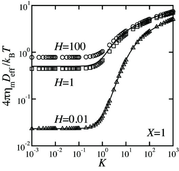
Figure 11: Scaled effective diffusion coefficient $4\pi\eta_{\rm m}D_{\rm eff}/k_{\rm B}T$ as a function of dimensionless wavenumber $K=k/\nu$. The dimensionless correlation length, $X=\xi\nu$, is fixed to unity, while $H=h\nu$ is the dimensionless distance between the membrane and the wall and its value varies between 0.01 to 100. Symbols are numerical calculations and the solid lines correspond to the analytical expression given in Ref. [86] obtained in the limit of small $H$.

In another study, Ramachandran et al. [88] used the general mobility tensor of Eq. (7) to numerically calculate the effective diffusion coefficient. This quantity includes several parameters such as the correlation length $\xi$, the hydrodynamic screening length $\nu^{-1}$, and the distance $h$ between the membrane and the wall. Their main findings are reproduced in Fig. 11 where we plot the computed effective diffusion coefficient $D_{\rm eff}$ as a function of the dimensionless wavenumber $K=k/\nu$. The dimensionless quantity $X=\xi\nu=1$ is held fixed, while $H=h\nu$ is varied between three representative values: $H=0.01,1,100$. The symbols correspond to the numerical estimates and the solid lines represent the analytical expression derived in Ref. [86]. For $K\ll 1$, we see that $D_{\rm eff}$ is almost a constant that depends on $H$, while it increases logarithmically for $K\gg 1$. Notice that this logarithmic dependence is a characteristic feature specific to 2d fluid membranes, and does not exist for 3d critical fluids [89].

7 2d microemulsion model

7.1 Hybrid lipids

One central issue in regards to lipid rafts in biomembranes is to identify the physical mechanism that determines the finite domain size. In this section, we discuss the possibility of having another length scale that is associated with rafts, and which is different from the correlation length $\xi$ discussed so far.

In Sec. 2 we mentioned various ternary lipid mixtures, such as DOPC/DPPC/ cholesterol that have been extensively studied. If we take a closer look at the DOPC and DPPC molecules, we note that for DOPC the two chains contain each one unsaturated bond (doubly unsaturated lipid), while for DPPC both chains are fully saturated. Other type of lipids such as POPC and SOPC has one unsaturated chain and one saturated chain. They are sometimes called "hybrid lipids". Real biomembranes contain a much larger fraction of hybrid lipids than doubly unsaturated ones such as DOPC [90].

Considering a mixture of doubly unsaturated lipid, saturated lipid, and hybrid lipid, we realize that this system resembles microemulsions — a well-studied 3d ternary liquid mixture composed of water/oil/surfactant. In microemulsions, surfactants are absorbed at water/oil interfaces and reduce the water/oil interfacial tension [91]. By analogy, we expect that hybrid lipids will play a similar role in 2d by absorbing at interfaces between the doubly-unsaturated lipids and the saturated lipids, in order to reduce the line tension. This effect can be referred to as "line activity" in 2d systems, and is similar to "surface activity" of surfactants in 3d.

A lattice model for this type of 2d microemulsion-like ternary mixtures has been proposed by Brewster et al. [92, 93]. In their model they calculated the reduction of the line tension due to the presence of hybrid lipid in small quantities. This lattice model for ternary mixtures has been recently further extended by Palmieriet al. [94, 95] for any fraction of unsaturated, saturated and hybrid lipids. It was shown that the correlation length of concentration fluctuations decreases dramatically with increasing amounts of hybrid lipids, and nanoscale fluctuations are more probable in the presence of hybrid lipids. In their second work [95], Palmieri et al. concluded that hybrid lipids increase the lifetime of fluctuations.

Yamamoto et al. et al. [96, 97] showed that, in some cases, the reduction of line tension is more pronounced than for three-component lipid mixtures. More details are provided by Palmieri et al. in a separate contribution to this special issue.

7.2 Coupling between concentration field and orientation field

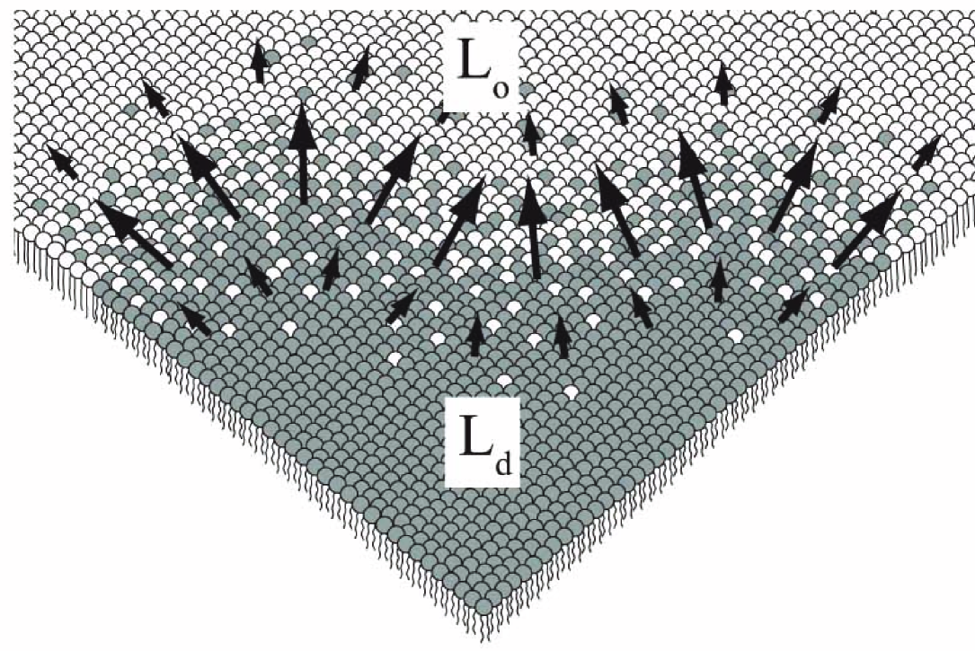
Figure 12: Lipid monolayer consisting of saturated lipids and hybrid lipids. The orientational vector field $\mathbf{m}$ points from the L_d-phase to the L_o-phase, and its magnitude becomes large at the interface between the two phases.

Hirose et al. [98, 99] extended the models by Brewster et al. [92, 93] and Yamamoto et al. [96, 97] first to lipid monolayers and then to coupled bilayers as will be discussed later. In their work they proposed a Ginzburg–Landau model for systems containing hybrid lipids in addition to saturated ones. They introduced a 2d orientational vector-field $\mathbf{m}({\mathbf{r}})$, which points from the unsaturated chain to the saturated chain of a hybrid lipid. As shown in Fig. 12, the orientational vector $\mathbf{m}$ is aligned toward the L_o-phase, and its magnitude increases at the interface. In addition to Eq. (13), the free energy has some additional terms [99]:

$$F[\mathbf{m},\phi]=\int{\rm d}{\mathbf{r}}\,\left[\frac{E}{2}(\nabla\cdot\mathbf{m})^{2}+\frac{b}{2}\mathbf{m}^{2}-\Lambda\mathbf{m}\cdot(\nabla\phi)\right],$$ (18)

where $E$ is the 2d elastic constant, and both $b$ and $\Lambda$ are positive coefficients.

The total free energy is the sum of Eqs. (13) and (18) can be minimized with respect to $\mathbf{m}({\mathbf{r}})$. It then results in effective monolayer free-energy that depends only $\phi$, and within the long-wavelength approximation the expression is:

$$F_{\rm m}[\phi]=\int{\rm d}{\mathbf{r}}\,\left[\frac{B}{2}(\nabla^{2}\phi)^{2}-\frac{A}{2}(\nabla\phi)^{2}+\frac{a}{2}\phi^{2}+\frac{1}{4}\phi^{4}\right],$$ (19)

where $B=E\Lambda^{2}/b^{2}$ and $A=\Lambda^{2}/b-c$. When the coupling coefficient $\Lambda$ is large enough, $A>0$, the above effective free-energy exhibits an instability at a finite wavenumber $k^{\ast}=\sqrt{A/2B}$ [100].

The 2d free-energy in Eq. (19) has the same form as that for 3d microemulsions [91]. The important dimensionless parameter is $\theta=-A/\sqrt{4aB}$ valid for $a>0$ ($T>T_{\rm c}$). When $|\theta|<1$, the correlation function, $G_{\phi\phi}(\mathbf{r})=\langle\delta\phi(\mathbf{r})\delta\phi(0)\rangle$, obtained from Eq. (19) decays with an oscillatory component. The correlation length and the period length are given by $\xi=(4B/a)^{1/4}(1+\theta)^{-1/2}$ and $\lambda/2\pi=(4B/a)^{1/4}(1-\theta)^{-1/2}$, respectively. Although both lengths are finite for $|\theta|<1$, $\xi$ diverges at $\theta=-1$ and $\lambda$ at $\theta=1$. When the correlation length $\xi$ diverges, micro-phase separated structures such as the stripe or hexagonal phases become more stable [91].

7.3 Curvature instability

Another physical mechanism which leads to very similar microemulsion-like free-energy is the curvature instability [37]. In this model, the concentration field is coupled to the membrane curvature. Within the Monge representation, the shape of a membrane can be described by its height $h({\mathbf{r}})$, and the curvature elasticity energy, Eq. (2), is given approximately by:

$$F[h,\phi]=\int{\rm d}{\mathbf{r}}\,\left[\frac{\kappa}{2}(\nabla^{2}h)^{2}+\frac{\Sigma}{2}(\nabla h)^{2}-\Upsilon(\nabla^{2}h)\phi\right],$$ (20)

where $\kappa$ is the bending rigidity introduced earlier, $\Sigma$ the membrane surface tension, and $\Upsilon$ is a coupling coefficient between local composition and curvature, while the term associated with the Gaussian curvature is neglected.

Physically speaking, the coupling term represents a spontaneous curvature that depends on the local concentration $\phi$. By adding Eqs. (13) and (20), one can minimize the total free-energy with respect to $h({\mathbf{r}})$, and obtain a free-energy similar to Eq. (19). Equilibrium shapes of modulated vesicles were investigated in detail in two limits: strong segregation limit (temperatures much smaller than the critical temperature) [38, 39], and weak segregation one (close to the critical temperature) [40].

For bilayers, in particular, the membrane curvature can be naturally coupled to the compositional asymmetry between the two leaflets, and it can also lead to a curvature instability [101, 102, 103, 104]. From the energetic point of view, the frustration to form bilayers out of two monolayers can be avoided by creating a composition asymmetry in binary membranes. Using this idea, Schick and co-workers proposed a free energy similar to Eq. (19) for bilayer membranes [105, 106], while Meinhardt et al. [107] considered the coupling effect between the curvature and the membrane thickness, which also results in the formation of modulated phases at low temperatures.

7.4 Coupled modulated monolayers

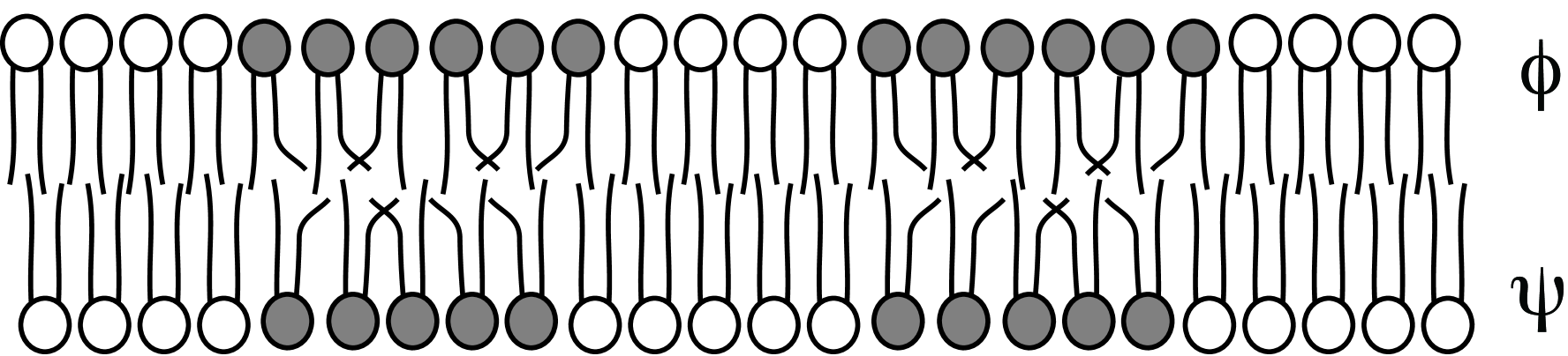
Figure 13: Schematic illustration of two coupled modulated monolayers of concentration $\phi$ (upper) and $\psi$ (lower) forming a bilayer membrane. Each monolayer is composed of a binary mixture of saturated lipid (white) and hybrid lipid (gray), which can have a lateral modulation in $\phi$ and $\psi$.

Hirose et al. [98, 99] considered bilayers composed of two modulated monolayers whose free energies are described by Eq. (19). Denoting the concentrations of the upper and lower leaflets by $\phi$ and $\psi$, respectively (see Fig. 13), the total bilayer free-energy is given by

$$F_{\rm b}[\phi,\psi]=\int{\rm d}{\mathbf{r}}\,\biggl{[} \frac{B_{\phi}}{2}(\nabla^{2}\phi)^{2}-\frac{A_{\phi}}{2}(\nabla\phi)^{2}+\frac{a_{\phi}}{2}\phi^{2}+\frac{1}{4}\phi^{4}$$

$$+ \frac{B_{\psi}}{2}(\nabla^{2}\psi)^{2}-\frac{A_{\psi}}{2}(\nabla\psi)^{2}+\frac{a_{\psi}}{2}\psi^{2}+\frac{1}{4}\psi^{4}-\Xi\phi\psi\biggr{]},$$ (21)

and is constructed from Eq. (19) for each monolayer. The coupling between the two leaflets is taken into account by the last term in which $\Xi$ is the coupling coefficient [21, 22, 23, 24, 25].

Above the transition temperature, both static and dynamic properties of concentration fluctuations have been investigated in Refs. [98, 99]. For example, the static partial structure factor $S_{\phi\phi}(\mathbf{k})=\langle\delta\phi(\mathbf{k})\delta\phi(-\mathbf{k})\rangle$ can be obtained by the 2d Fourier transform of the correlation function $G_{\phi\phi}(\mathbf{r})=\langle\delta\phi(\mathbf{r})\delta\phi(0)\rangle$ as introduced before. Similarly, the other partial structure factors, $S_{\psi\psi}(\mathbf{k})$ and $S_{\phi\psi}(\mathbf{k})$, can be obtained.

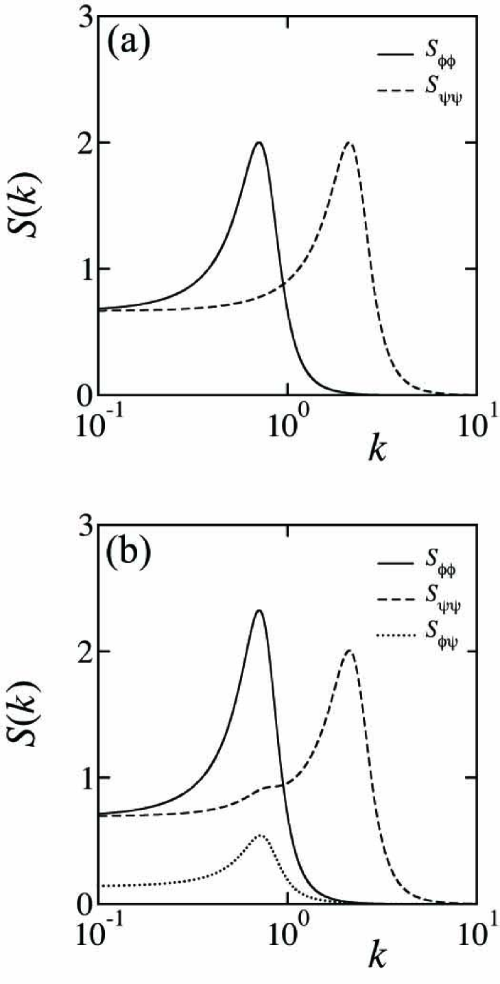
Figure 14: Bilayer structure factors $S_{\phi\phi}$, $S_{\psi\psi}$, and $S_{\phi\psi}$ as a function of the wavenumber $k$. (a) The decoupled case, $\Xi=0$. (b) The coupled case with $\Xi=0.3$.

In Fig. 14(a) and (b), we plot the structure factors of the decoupled and coupled cases, respectively. As an illustration of the coupling effect, we consider that the $\phi$ and $\psi$ leaflets have different characteristic wavenumbers [94]: $k_{\phi}^{*}<k_{\psi}^{*}$, while the heights of the two peaks are set to be equal. The peak height of $S_{\phi\phi}$ at $k_{\phi}^{*}$ is increased due to the coupling effect, whereas that of $S_{\psi\psi}$ at $k_{\psi}^{*}$ is almost unchanged, as compared with the decoupled case. We also plot $S_{\phi\psi}$ that represents the cross-correlation of fluctuations between the two leaflets. This quantity is proportional to the coupling constant $\Xi$ and its peak position is essentially determined by that of $S_{\phi\phi}$ at $k_{\phi}^{*}$.

The dynamical fluctuations in composition, $\delta\phi(\mathbf{r},t)$ and $\delta\psi(\mathbf{r},t)$, are also considered for coupled modulated monolayers [98, 99]. Since the exchange of lipids between the two monolayers is negligible, the time evolution of $\delta\phi$ and $\delta\psi$ are given by the diffusive equations (in the absence of any hydrodynamic effects). In the decoupled case, one can show that the $S_{\phi\phi}$ and $S_{\psi\psi}$ structure factors decay with a single exponential characterized by a decay rate that depends on the wavenumber. For nonzero coupling coefficient, $\Xi\neq 0$, it was shown that the decay of concentration fluctuations is described by a sum of two exponentials. Generally speaking, the coupling affects the decay time of the leaflet with the smaller wavenumber (larger length scale).

Below the transition temperature when both monolayers exhibit micro-phase separation and form either stripe (S) or hexagonal (H) phase, the leaflet coupling brings about various combinations of the monolayer modulated phases. When the two leaflets have the same preferred periodicity, $k_{\phi}^{*}=k_{\psi}^{*}$, Hirose et al. [98] obtained the mean-field phase diagram exhibiting various combinations of modulated structures. In some cases, the periodic structure in one of the monolayers induces a similar modulation in the second monolayer. Moreover, the region of the induced modulated phase expands as the coupling parameter $\Xi$ becomes larger.

When the preferred periodicity of the two leaflets is different, $k_{\phi}^{*}\neq k_{\psi}^{*}$, it is necessary to solve numerically the coupled time-evolution equations given by

$$\frac{\partial\phi}{\partial t}=L_{\phi}\nabla^{2}\frac{\delta F_{\rm b}}{\delta\phi},$$

$$\frac{\partial\psi}{\partial t}=L_{\psi}\nabla^{2}\frac{\delta F_{\rm b}}{\delta\psi},$$ (22)

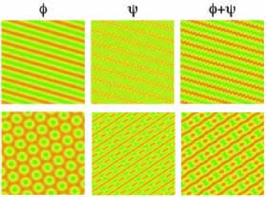
Figure 15: Patterns of two coupled modulated leaflets of concentration $\phi$ and $\psi$. In the three top parts the $\phi$ and $\psi$ leaflets consist of a stripe phase, while in the three bottom parts the coupling is between hexagonal (in $\phi$) and stripe (in $\psi$) phases, each having a different characteristic wavelength. Left: $\phi$-monolayer, middle: $\psi$-monolayer, and right: $\phi+\psi$.

where the bilayer free-energy, $F_{\rm b}[\phi,\psi]$, is given by Eq. (21). It was shown [98, 99] that various complex patterns are formed due to the frustration between the two incommensurate modulated structures. In Fig. 15, we show examples of complex patterns created from two stripe structures (top), or stripe and hexagonal structures (bottom). Broadly speaking, the structure with the larger wavelength dominates when the coupling is large enough, which is in accord with the properties of the static structure factors. More details are discussed in Refs. [98, 99].

8 Outlook

In this article, we reviewed some of the more recent physical and chemical-physics studies concerning the static and dynamic properties of lateral phase-separation in multi-component lipid bilayers. We intentionally avoided including other studies based on biological perspectives as we preferred to keep this review focused on physical concepts and their impact on the understanding of biomembranes.

We have shown that even for the simplified case of lipid membranes composed of only three components, the inhomogeneity in the lateral composition couples with the membrane shape, and can lead to a rich variety of interesting phenomena. We believe that purely physical phenomena such as phase separation and diffusion that occur in biomembranes may play an important role in biological systems. Since these physical phenomena can be described using appropriate and well-defined physical models, more quantitative arguments are possible regarding the static and dynamic features of lipid domains and, presumingly, with an impact on rafts.

It will be of interest to explore in the future the phase separation in multi-component lipid membranes in presence of glycolipids and membrane proteins, because the latter are abundant in biomembranes [108]. Understanding the interactions between protein molecules embedded inside multi-component membranes [109], as well as between different multi-component membranes would be also of interest for future investigations [110].

References

- [1] B. Alberts, A. Johnson, P. Walter, J. Lewis and M. Raff, Molecular Biology of the Cell, 5th ed. (Garland Science, New York, 2008).
- [2] S. J. Singer and G. L. Nicolson, Science 175 (1972) 720.
- [3] K. Simons and E. Ikonen, Nature 387 (1997) 569.
- [4] L. J. Pike, J. Lipid Research 47 (2006) 1597.
- [5] M. Leslie, Science 334 (2011) 1046.
- [6] R. Lipowsky and E. Sackmann, Structure and Dynamics of Membranes (Elsevier, Amsterdam, 1995).
- [7] J. H. Ipsen, G. Karlström, O. G. Mourtisen, H. Wennerström and M. J. Zuckermann, Biochim. Biophys. Acta 905 (1987) 162.
- [8] C. Dietrich, L. A. Bagatolli, Z. N. Volovyk, N. L. Thompson, M. Levi, K. Jacobson and E. Gratton, Biophys. J. 80 (2000) 1417.
- [9] S. L. Veatch and S. L. Keller, Phys. Rev. Lett. 89 (2002) 268101.
- [10] S. L. Veatch and S. L. Keller, Biophys. J. 85 (2003) 3074.
- [11] S. L. Veatch and S. L. Keller, Phys. Rev. Lett. 94 (2005) 148101.
- [12] H. J. Risselada and S. J. Marrink, Proc. Natl. Acad. Sci. U.S.A. 105 (2008) 17367.
- [13] S. L. Veatch, K. Gawrisch and S. L. Keller, Biophys. J. 90 (2006) 4428.
- [14] P. G. de Gennes and J. Prost, The Physics of Liquid Crystals (Oxford Univ. Press, New York, 1993).
- [15] S. Komura, H. Shirotori, P. D. Olmsted and D. Andelman, Europhys. Lett. 67 (2004) 321.
- [16] S. Komura, H. Shirotori and P. D. Olmsted, J. Phys.: Condens. Matter 17 (2005) S2951.
- [17] R. Elliott, I. Szleifer and M. Schick, Phys. Rev. Lett. 96 (2006) 098101.
- [18] G. G. Putzel and M. Schick, Biophys. J. 95 (2008) 4756.
- [19] J. Wolff, C. M. Marques and F. Thalmann, Phys. Rev. Lett. 106 (2011) 128104.
- [20] A. Zachowski, Biochem. J. 294 (1993) 1.
- [21] M. D. Collins, Biophys. J. 94 (2008) L32.
- [22] S. May, Soft Matter 5 (2009) 3148.
- [23] M. D. Collins and S. L. Keller, Proc. Natl. Acad. Sci. U.S.A. 105 (2008) 124.
- [24] A. J. Wagner, S. Loew and S. May, Biophys. J. 93 (2007) 4268.
- [25] G. G. Putzel and M. Schick, Biophys. J. 94 (2008) 869.
- [26] W. Helfrich, Z. Naturforsch. 28c (1973) 693.
- [27] S. Svetina and B. Zeks, Biochim. Biophys. Acta 42 (1983) 86.
- [28] L. Miao, U. Seifert, M. Wortis and H.-G. Döbereiner, Phys. Rev. E 49 (1994) 5389.
- [29] R. Lipowsky, J. Phys. II France 2 (1992) 1825.
- [30] F. Jülicher and R. Lipowsky, Phys. Rev. Lett. 70 (1993) 2964.
- [31] F. Jülicher and R. Lipowsky, Phys. Rev. E 53 (1996) 2670.
- [32] T. Baumgart, S. T. Hess and W. W. Webb, Nature 425 (2003) 821.
- [33] T. Baumgart, S. Das, W. W. Webb and J. T. Jenkins, Biophys. J. 89 (2005) 1067.
- [34] I. W. Hamley, The Physics of Block Copolymers (Oxford University Press, Oxford, 1998).
- [35] T. Konyakhina, S. Goh, J. Amazon, F. Heberle, J. Wu and G. Feigenson, Biophys. J. 101 (2011) L08.
- [36] M. Yanagisawa, N. Shimokawa, M. Ichikawa and K. Yoshikawa, Soft Matter 8 (2012) 488.
- [37] S. Leibler and D. Andelman, J. Phys. (Paris) 48, (1987) 2013.
- [38] D. Andelman, T. Kawakatsu and K. Kawasaki, Europhys. Lett. 19, (1992) 57.
- [39] T. Kawakatsu, D. Andelman, K. Kawasaki and T. Taniguchi, J. Phys. II (France) 3, (1993) 971.
- [40] T. Taniguchi, K. Kawasaki, D. Andelman and T. Kawakatsu, J. Phys. II (France) 4, (1994) 1333.
- [41] M. Yanagisawa, M. Imai and T. Taniguchi, Phys. Rev. Lett. 100 (2008) 148102.
- [42] N. Shimokawa, M. Hishida, H. Seto and K. Yoshikawa, Chem. Phys. Lett. 496 (2010) 59.
- [43] N. Shimokawa, S. Komura and D. Andelman, Phys. Rev. E 84 (2011) 031919.
- [44] P. G. Saffman and M. Delbrück, Proc. Natl. Acad. Sci. U.S.A. 72 (1975) 3111.
- [45] P. G. Saffman, J. Fluid Mech. 73 (1976) 593.
- [46] L. D. Landau and E. M. Lifshitz, Fluid Mechanics (Pergamon Press, Oxford, 1987).
- [47] S. Ramachandran, S. Komura, K. Seki and G. Gompper, Eur. Phys. J. E 34 (2011) 46.
- [48] K. Seki, S. Ramachandran and S. Komura, Phys. Rev. E 84 (2011) 021905.
- [49] N. Oppenheimer and H. Diamant, Biophys. J. 96 (2009) 3041.
- [50] N. Oppenheimer and H. Diamant, Phys. Rev. E 82 (2010) 041912.
- [51] B. D. Hughes, B. A. Pailthorpe and L. R. White, J. Fluid Mech. 110 (1981) 349.
- [52] P. Cicuta, S. L. Keller and S. L. Veatch, J. Phys. Chem. B 111 (2007) 3328.
- [53] E. Evans and E. Sackmann, J. Fluid Mech. 194 (1988) 553.
- [54] K. Seki and S. Komura, Phys. Rev. E 47 (1993) 2377.
- [55] S. Komura and K. Seki, J. Phys. II 5 (1995) 5.
- [56] S. Ramachandran, S. Komura, M. Imai and K. Seki, Eur. Phys. J. E 31 (2010) 303.
- [57] H. Stone and A. Ajdari, J. Fluid Mech. 369 (1998) 151.
- [58] S. Komura, S. Ramachandran and K. Seki, EPL 97 (2012) 68007.
- [59] S. Komura, S. Ramachandran and K. Seki, Materials 5 (2012) 1923.
- [60] A. V. Weigel, B. Simon, M. M. Tamkun and D. Krapf, Proc. Natl. Acad. Sci. U.S.A. 108 (2011) 6438.
- [61] D. Saeki, T. Hamada and K. Yoshikawa, J. Phys. Soc. Jpn. 75 (2006) 013602.
- [62] M. Yanagisawa, M. Imai, T. Masui, S. Komura and T. Ohta, Biophys. J. 92 (2007) 115.
- [63] C. A. Stanich, A. R. Honerkamp-Smith, G. G. Putzel, C. S. Warth, A. K. Lamprecht, P. Mandal, E. Mann, T.-A. D. Hua and S. L. Keller, Biophys. J. 105 (2013) 444.
- [64] T. Taniguchi, Phys. Rev. Lett. 76 (1996) 4444.
- [65] P. B. Sunil Kumar, G. Gompper and R. Lipowsky, Phys. Rev. Lett. 86 (2001) 3911.
- [66] G. S. Ayton, J. L. McWhirter, P. McMurtry and G. A. Voth, Biophys. J. 88 (2005) 3855.
- [67] R. D. Groot and P. B. Warren, J. Chem. Phys. 107 (1997) 4423.
- [68] M. Laradji and P. B. Sunil Kumar, Phys. Rev. Lett. 93 (2004) 198105.
- [69] M. Laradji and P. B. Sunil Kumar, J. Chem. Phys. 123 (2005) 224902.
- [70] S. Ramachandran, S. Komura and G. Gompper, EPL 89 (2010) 56001.
- [71] P. M. Chaikin, T. C. Lubensky, Principles of Condensed Matter Physics (Cambridge University Press, Cambridge, 1995).
- [72] P. C. Hohenberg and I. Halperin, Rev. Mod. Phys. 49 (1977) 435.
- [73] B. A. Camley and F. L. H. Brown, J. Chem. Phys. 135 (2011) 225106.
- [74] J. Fan, T. Han and M. Haataja, J. Chem. Phys. 133 (2010) 235101.
- [75] E. M. Lifshitz and L. P. Pitaevskii, Physical Kinetics (Pergamon Press, Oxford, 1981).
- [76] P. Sens and M. S. Turner, Phys. Rev. Lett. 106 (2011) 238101.
- [77] L. Foret, Eur. Phys. J. E 35 (2012) 12.
- [78] L. Foret, Europhys. Lett. 71 (2005) 508.
- [79] J. Fan, M. Sammalkorpi and M. Haataja, Phys. Rev. E 81 (2010) 011908.
- [80] J. Gómez, F. Sagués and R. Reigada, Phys. Rev. E 80 (2009) 011920.
- [81] T. Hamada, R. Sugimoto, T. Nagasaki and M. Takagi, Soft Matter 7 (2011) 220.
- [82] S. L. Veatch, O. Soubias, S. L. Keller and K. Gawrisch, Proc. Natl. Acad. Sci. U.S.A. 104 (2007) 17650.
- [83] A. R. Honerkamp-Smith, P. Cicuta, M. Collins, S. L. Veatch, M. Schick, M. den Nijs and S. L. Keller, Biophys. J. 95 (2008) 236.
- [84] S. L. Veatch, P. Cicuta, P. Sengupta, A. R. Honerkamp-Smith, D. Holowka and B. Baird, ACS Chem. Biol. 3 (2008) 287.
- [85] A. R. Honerkamp-Smith, B. B. Machta and S. L. Keller, Phys. Rev. Lett. 108 (2012) 265702.
- [86] K. Seki, S. Komura and M. Imai, J. Phys.: Condens. Matter 19 (2007) 072101.
- [87] K. Inaura and Y. Fujitani, J. Phys. Soc. Jpn. 77 (2008) 114603.
- [88] S. Ramachandran, S. Komura, K. Seki and M. Imai, Soft Matter 7 (2011) 1524.
- [89] K. Kawasaki, Ann. Phys. 61 (1970) 1.
- [90] G. van Meer, D. Voelker and G. Feigenson, Nature Rev. Mol. Cell. Biol. 9 (2008) 112.
- [91] G. Gompper and M. Schick, Self-Assembling Amphiphilic Systems (Academic, New York, 1994).
- [92] R. Brewster, P. A. Pincus and S. A. Safran, Biophys. J. 97 (2009) 1087.
- [93] R. Brewster and S. A. Safran, Biophys. J. 98 (2010) L21.
- [94] B. Palmieri and S. A. Safran, Langmuir 29 (2013) 5246.
- [95] B. Palmieri and S. A. Safran, Phys. Rev. E 88 (2013) 032708.
- [96] T. Yamamoto, R. Brewster and S. A. Safran, EPL 91 (2010) 28002.
- [97] T. Yamamoto and S. A. Safran, Soft Matter 7 (2011) 7021.
- [98] Y. Hirose, S. Komura and D. Andelman, ChemPhysChem 10 (2009) 2839.
- [99] Y. Hirose, S. Komura and D. Andelman, Phys. Rev. E 86 (2012) 021916.
- [100] S. Brazovskiĭ, Sov. Phys. JETP 41 (1975) 85.
- [101] S. A. Safran, P. A. Pincus, D. Andelman and F. C. MacKintosh, Phys. Rev. A 43, (1991) 1071.
- [102] F. C. MacKintosh and S. A. Safran, Phys. Rev. E 47, (1993) 1180.
- [103] H. Kodama and S. Komura, J. Phys. II (France) 3, (1993) 1305.
- [104] P. B. Sunil Kumar, G. Gompper and R. Lipowsky, Phys. Rev. E 60, (1999) 4610.
- [105] M. Schick, Phys. Rev. E 85 (2012) 031902.
- [106] R. Shlomovitz and M. Schick, Biophys. J. 105 (2013) 1406.
- [107] S. Meinhardt, R. L. C. Vink and F. Schmid, Proc. Natl. Acad. Sci. U.S.A. 110 (2013) 4476.
- [108] K. G. N. Suzuki, R. S. Kasai, K. M. Hirosawa, Y. L. Nemoto, M. Ishibashi, Y. Miwa, T. K. Fujiwara and A. Kusumi, Nature Chem. Biol. 8 (2012) 774.
- [109] B. J. Reynwar and M. Deserno, Biointerphases 3 (2008) 117.
- [110] S. Komura and D. Andelman, Europhys. Lett. 64 (2003) 844.