Singularities around the QCD critical point in the complex chemical potential plane

Abstract:

We consider thermodynamic singularities appearing in the complex chemical potential plane in the vicinity of QCD critical point. In order to investigate what the singularities are like in a concrete form, we resort to an effective theory based on a mean filed approach. We study the behavior of extrema of the real part of the complex effective potential in the complex order parameter plane.

1 Introduction

In this talk, we report on thermodynamic singularities of QCD in the vicinity of the QCD critical point (CP) [1, 2, 3] in the complex chemical potential ($\mu$) plane. This issue is deeply connected with zeros of the partition function. Study of them provides an alternative approach to the critical phenomena and its scaling behaviors [4, 5, 6, 7, 8, 9, 10, 11, 12, 13, 14]. At finite volume, the zeros are scattered in the complex $\mu$ plane, and as the volume increases, the zeros accumulate on curves. In the infinite volume limit, the zeros cross the real $\mu$ axis at the critical point and the singularity appears on the real axis. Off the critical point, the singularities moves into the complex plane, and the curve of zeros called the Stokes line [15] is connected to the singularity.

In order to investigate what the singularities are like in the vicinity of the CP, we make use of an effective theory [16, 17] reflecting the phase structure around the CP. This model [16] is constructed based on the tricritical point (TCP) in the $\mu$-T plane in the chiral limit, which has the upper critical dimension equal to 3, and thus its mean field description is expected to be valid up to a logarithmic correction. Above the critical temperature, the singularities are located off the real $\mu$ axis, and thus a reminiscence of the singularity appears on the real axis as a crossover.

With complex $\mu$, the order parameter becomes complex and so does the effective potential. Its $\mu$ dependence is quite intricate. The simplicity of the model, however, allows to analyze the complex potential. We explicitly trace extrema of the real part of the potential. In the vicinity of the singularity, their movements show different behaviors depending on where they pass. From its behaviors, we identify where the Stokes lines are located.

In the following section, we briefly explain the model, and the results are shown in section 3. In section 4, summary is presented.

2 Model

Let us briefly explain the model [16] which we deal with in this report. We consider two-flavor case. In the chiral limit, there exists a TCP at finite temperature and density, which is connected to a O(4) critical point at $\mu=0$ along a critical line [18]. A first order line goes down from the TCP toward lower temperature side. When quark mass $m$ is introduced, the critical line is absent, and the surviving first order line terminates at a critical point (CP). This CP can be described by fluctuations of the sigma meson and is expected to share the same universality with 3-d Ising model [19]. Since the upper critical dimension of the tricritical point is equal to 3, the TCP in QCD phase diagram can be described by a mean field theory up to a logarithmic correction. As far as $m$ is small, the universal behavior around the CP is also expected to be described in the mean field framework.

Starting with the Landau-Ginzburg potential

$$\Omega_{LG}=-m\sigma+\frac{a}{2}\sigma^{2}+\frac{b}{4}\sigma^{4}+\frac{c}{6}\sigma^{6},$$ (1)

one expands the coefficients around the tricritical point (TCP) ($a=b=m=0$) as $a(T,\mu)=C_{a}(T-T_{3})+D_{a}(\mu-\mu_{3}),\ b(T,\mu)=C_{b}(T-T_{3})+D_{b}(\mu-\mu_{3}),$ where ($\mu_{3},T_{3}$) denotes temperature and chemical potential at the TCP, respectively. The coefficients $C$ and $D$ are constrained to some extent reflecting the structure around the TCP, i.e., $C_{b}D_{a}-C_{a}D_{b}>0\ (C_{a},C_{b},D_{a},D_{b}>0)$ [16]. By switching on $m$, the CP exists at $T=T_{E}$ and $\mu=\mu_{E}$ so that $\Omega^{{}^{\prime}}(T_{E},\mu_{E},\sigma_{0})=\Omega^{{}^{\prime\prime}}(T_{E},\mu_{E},\sigma_{0})=\Omega^{{}^{\prime\prime\prime}}(T_{E},\mu_{E},\sigma_{0})=0\ (\Omega^{{}^{\prime}}\equiv\partial\Omega/\partial\sigma),$ which leads to the coefficients $a(T_{E},\mu_{E})=9b^{2}(T_{E},\mu_{E})/(20c)$, and $-b(T_{E},\mu_{E})=(5/54^{1/5})c^{3/5}m^{2/5},$ and expectation value of $\sigma$; $\sigma_{0}=\sqrt{-3\ b(T_{E},\mu_{E})/(10c)}.$ Expanding $\Omega(T,\mu,\sigma)$ around $\Omega(T_{E},\mu_{E},\sigma_{0})$, we obtain thermodynamic potential around the CP given by

$$\Omega(T,\mu,\sigma)=\Omega(T_{E},\mu_{E},\sigma_{0})+A_{1}\hat{\sigma}+A_{2}\hat{\sigma}^{2}+A_{3}\hat{\sigma}^{3}+A_{4}\hat{\sigma}^{4}+\mathit{O}({\hat{\sigma}}^{5}),$$ (2)

where $\hat{\sigma}=\sigma-\sigma_{0}$. The coefficients $A_{i}$ are given as follows as a function of $T$ and $\mu$.

$$A_{1} = \left(C_{a}\sigma_{0}+C_{b}\sigma_{0}^{3}\right)\tilde{t}_{E}+\left(D_{a}\sigma_{0}+D_{b}\sigma_{0}^{3}\right)\tilde{\mu}_{E}$$

$$A_{2} = \frac{1}{2}\left(C_{a}+3C_{b}\sigma_{0}^{3}\right)\tilde{t}_{E}+\frac{1}{2}\left(D_{a}+3D_{b}\sigma_{0}^{3}\right)\tilde{\mu}_{E}$$

$$A_{3} = \left\{C_{b}\tilde{t}_{E}+D_{b}\tilde{\mu}_{E}\right\}\sigma_{0}$$

$$A_{4} = -\frac{b(T_{E},\mu_{E})}{2}+\frac{1}{4}\left(C_{b}\tilde{t}_{E}+D_{b}\tilde{\mu}_{E}\right),$$ (3)

where $\tilde{t}_{E}\equiv T-T_{E}$ and $\tilde{\mu}_{E}\equiv\mu-\mu_{E}$.

3 Results

3.1 Singular points

Using the potential in Eq. (2), the instability of the extrema occurs at such $\sigma$ that

$$\frac{\partial\Omega}{\partial\sigma}=0,\quad\frac{\partial^{2}\Omega}{\partial\sigma^{2}}=0$$ (4)

are simultaneously satisfied. Namely,

$$A_{1}+2A_{2}\sigma+3A_{3}\sigma^{2}+4A_{4}\sigma^{3}=0,\quad 2A_{2}+6A_{3}\sigma+12A_{4}\sigma^{2}=0.$$ (5)

The discriminant of the left equation in Eq.(5) is solved as a function of $\tilde{\mu}_{E}$ and $\tilde{t}_{E}$ to obtain the singular points $\tilde{\mu}_{E}^{(s)}$.

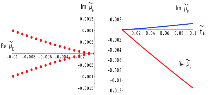
Figure 1: Left: Singularities in the complex $\tilde{\mu}_{E}=\mu-\mu_{E}$ plane. $C_{a}=0.1$ and $x_{m}=m^{1/5}=0.2$. The other parameters are $C_{b}=D_{a}=D_{b}=c=1.0$. Temperatures are chosen to be $\tilde{t}_{E}=T-T_{E}=0,0.005,0.01,0.15,0.02,\cdots,0.09$. Right: The $\tilde{t}_{E}$-dependence of Re $\tilde{\mu}_{E}^{(s)}$ (red) and Im $\tilde{\mu}_{E}^{(s)}$ (blue). Re $\tilde{\mu}_{E}^{(s)}$ is linear in $\tilde{t}_{E}$, while Im $\tilde{\mu}_{E}^{(s)}$ behaves as $\tilde{t}_{E}^{3/2}$.

The left panel of Fig. 1 indicates the locations of ${\tilde{\mu}}^{(s)}_{E}$ in the complex $\tilde{\mu}_{E}$ plane for various values of temperature ($\tilde{t}_{E}\geq 0$). Throughout this report, $C_{a}=0.1$ and $C_{b}=D_{a}=D_{b}=c=1.0$ and $x_{m}=m^{1/5}=0.2$ are chosen for calculations. Temperatures are chosen to be $\tilde{t}_{E}=T-T_{E}=0,0.005,0.01,0.15,0.02,\cdots,0.09$. At $\tilde{t}_{E}=0$, the singularity of the CP appears on the real $\tilde{\mu}_{E}$ axis (the origin in the figure). For $\tilde{t}_{E}>0$, the singularities appearing in pairs deviate from the real $\tilde{\mu}_{E}$ axis as $\tilde{t}_{E}$ increases. The $\tilde{t}_{E}$-dependence of Re $\tilde{\mu}_{E}^{(s)}$ and Im $\tilde{\mu}_{E}^{(s)}$ is shown in the right panel. The real part depends linearly on $\tilde{t}_{E}$, while the imaginary one behaves as $\tilde{t}_{E}^{3/2}$ as expected [15].

3.2 Extrema of the complex effective potential

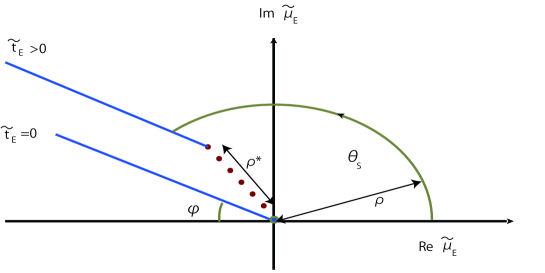
Figure 2: Stokes lines (blue) in the complex $\tilde{\mu}_{E}$ plane. The singular point $\tilde{\mu}_{E}^{(s)}$ for $\tilde{t}_{E}=0$ is located at the origin, while for $\tilde{t}_{E}>0$ one of complex pair of $\tilde{\mu}_{E}^{(s)}$ is shifted to the negative ${\rm Re}\tilde{\mu}_{E}$ direction in the upper half plane. Angle $\varphi$ is defined from the negative side of ${\rm Re}\tilde{\mu}_{E}$ axis.

In the present system, the critical point exists at $\tilde{\mu}_{E}=0$ for $\tilde{t}_{E}=0$, while for $\tilde{t}_{E}>0$ the singular point is shifted into the complex plane $\tilde{\mu}_{E}^{(s)}=\rho^{(s)}e^{i\theta^{(s)}}$ ($\rho^{(s)}>0$) as shown in Fig. 2, where only the upper half plane is shown. Let us move $\tilde{\mu}_{E}$ from a point on the real axis ($\tilde{\mu}_{E}>0$) to the other side at $\tilde{\mu}_{E}<0$ by changing $\theta$ from 0 to $\pi$ in $\tilde{\mu}_{E}=\rho e^{i\theta}$ for a fixed value of $\rho$. As the parameter is analytically continued from the one phase to the other, the corresponding global minimum of the potential is also analytically continued.

In order to explicitly see how this occurs, we take $\tilde{t}_{E}=0.1$. At this temperature, the singular points are located at $\tilde{\mu}_{E}^{(s)}=-0.0115\pm i\ 0.0012$ and thus $\rho^{(s)}=0.0116$. The left panel of Fig. 3 shows behaviors of the positions of three extrema of ${\rm Re}\ \Omega$ in the complex $\sigma$ plane as $\theta$ varies from $0$ to $\pi$ with a fixed value of $\rho$ $(=0.05)$. For $\theta=0$, ${\rm Re}\ \Omega$ develops three extrema at $\sigma=0.0108$ (A) and $\sigma=0.12910-i\ 0.4544$ (B) and $0.12910+i\ 0.4544$ (C), each of which is located at the initial point of the arrows denoted by A, B and C, respectively. The arrows in the figure indicate the direction of the movement of the three as $\theta$ varies from 0 to $\pi$. The extremum A, which is a global minimum for $\theta=0$, ends up with negative small value of $\sigma=-0.0366$ at $\theta=\pi$, while B does with the real axis at $\sigma=0.5848$, which is identified as the global minimum of $\Omega$ for $\theta=\pi$ from its shape. So the two extrema A and B are associated with the global minimum of $\Omega$ for real $\mu$, the phase for $\tilde{\mu}_{E}>0$ and the one for $\tilde{\mu}_{E}<0$ , respectively, while the extremum C is not associated with the phase transition. In this case, a discrete change occurs from one minimum to the other between $\theta=0$ and $\pi$, where

$${\rm Re}\ \Omega(\sigma_{+}) = {\rm Re}\ \Omega(\sigma_{-}),$$ (6)

is fulfilled, where $\sigma_{+}(\sigma_{-})$ is the location of the extremum analytically continued from $\tilde{\mu}_{E}>0$ ($\tilde{\mu}_{E}<0$ ). For $\rho=0.05$, it occurs at at $\theta=\theta_{S}=2.492=0.793\ \pi$ as shown in the right panel of Fig. 3, where their slopes show a discontinuity in accordance with the interpretation that the distribution of the partition function zeros can be regarded as that of the charges in analogy with two dimensional Coulomb gas [4, 15].

As $\rho$ decreases, the two extrema A and B approach each other, and for $\rho=\rho^{(s)}$, the two trajectories meet together at $\sigma^{(s)}$, where $\sigma^{(s)}$ is the minimum of ${\rm Re}\ \Omega$ for $\tilde{\mu}_{E}$ corresponding to the singularity, $\tilde{\mu}_{E}^{(s)}$ i.e., fulfilling the condition Eq. (4). In the case of $\tilde{t}_{E}=0.1$, $\tilde{\mu}_{E}^{(s)}=-0.0115+i\ 0.0012$, and $\sigma^{(s)}=0.1219-i\ 0.0653$. For further smaller value of $\rho<\rho^{(s)}$, only a single extremum A is associated with analytic continuation from $\tilde{\mu}_{E}>0$ to $\tilde{\mu}_{E}<0$. The other two extrema do not play a role for vacua.

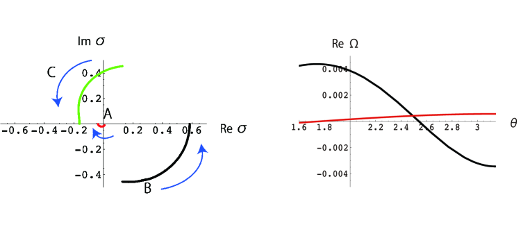
Figure 3: Left: Behaviors of the positions of three extrema of ${\rm Re}\ \Omega$ in the complex $\sigma$ plane as $\tilde{\mu}_{E}=\rho e^{i\theta}$ varies from $\theta=0$ to $\theta=\pi$ ($\rho=0.05$) for $\tilde{t}_{E}=0.1$. Right: Corresponding behaviors of Re $\Omega$ for the two extrema A (red) and B (black) as a function of $\theta$. The two values agree at $\theta_{S}=2.492$.

3.3 Stokes lines

In the case of $\tilde{t}_{E}>0$, therefore, the Stokes line runs for $\rho>\rho^{(s)}$. Figure 4 indicates how the Stokes line emanates from the singular point $\tilde{\mu}_{E}^{(s)}$ in the complex $\tilde{\mu}_{E}$ plane. Squared symbols indicate the locations which are calculated in the way described above, i.e., by choosing several value of $\rho$, tracing trajectories of the positions of the extrema upon varying $\theta$ and checking the behaviors of Re $\Omega$. For $\tilde{t}_{E}=0.2$, the singular point is located at $\tilde{\mu}_{E}^{(s)}$$=-0.02221+i\ 0.00254$ (black filled circle), and the Stokes line is alined on a straight line, which is tilted with angle $\varphi=\pi/4$ from an axis parallel to the negative axis of ${\rm Re}\tilde{\mu}_{E}$. As $\tilde{t}_{E}$ decreases, $\tilde{\mu}_{E}^{(s)}$ approaches the origin, and the angle $\varphi$ shows a increasing tendency. Green filled squares show the locations of the Stokes line for $\tilde{t}_{E}=0$. In this case the Stokes line emanates from the origin with $\varphi=\pi/2$.

For $\tilde{t}_{E}=-0.2$, a first order phase transition is located at $\tilde{\mu}_{E}=0.05553$, and the Stokes line goes out upright with $\varphi=\pi/2$ . In recent Monte Carlo study [20] of low temperature and high density QCD, the distribution of the Lee-Yang zeros have been calculated, and it looks similar to the behavior in the case of $\tilde{t}_{E}<0$ ($\varphi=\pi/2$), suggesting a possible first order phase transition.

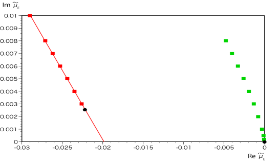
Figure 4: Locations of the Stokes line in complex $\tilde{\mu}_{E}$ plane, which are calculated by the trajectories of the two extrema of ${\rm Re}\ \Omega$ for $\tilde{t}_{E}=0.2$ (red) and $\tilde{t}_{E}=0$ (green). For $\tilde{t}_{E}=0.2$, it is clearly seen that thus identified points sit on a straight line with the slope $-1.09\pm 0.02$. Black symbol denotes the locations of the singular points $\tilde{\mu}_{E}^{(s)}$ $=-0.02221+i\ 0.00254$. For $\tilde{t}_{E}=0$, the singularity corresponding to the CP is situated at the origin. In this case the Stokes line emanates from the origin with $\varphi=\pi/2$.

4 Summary

We have discussed the thermodynamic singularities in the complex chemical potential plane in QCD at finite temperature and finite densities. For this purpose, we adopted an effective theory incorporating fluctuations around the CP. Singularities in the complex chemical potential plane are identified as unstable points of the extrema of the complex effective potential. At CP temperature, the singularity is located on the real $\mu$ axis, and above CP temperature it moves away from the real axis leaving its reminiscence as a crossover. Some phenomena on the real axis are then deeply connected with the singularity associated with the CP. Study of this aspect will be reported elsewhere [22]. Simplicity of the model allows us to explicitly deal with the complex potential as a function of the complex order parameter and complex $\mu$. We have had a close look at the behavior of the extrema of ${\rm Re}\ \Omega(\sigma)$ in the complex order parameter plane. It is found that two relevant extrema make a rearrangement at the singular point under the variation of $\mu$ around the singularity in the complex $\mu$ plane. It is also explicitly seen that the Stokes lines are located in the different way depending on temperature, higher or lower than the CP temperature or at the CP temperature. This provides us with information as to where the Lee-Yang zeros are located for finite volume.

It may be worth while to quantify what is described here. In [21], singularities of two-flavor QCD with staggered quarks have been investigated by having a look at the effective potential with respect to the plaquette variable. In order to have a more contact with the present report, some refinement of the computation would be necessary. This is now in progress  [23].

References

- [1] M. Asakawa and K. Yazaki, Nucl. Phys. A 504, 668 (1989).
- [2] A. Barducci, R. Casalbuoni, S. D. Curtis, R. Gatto and G. Pettini, Phys. Lett. B 231, 463 (1989).
- [3] J. Berges and K. Rajagopal, Nucl. Phys. B 538, 215 (1999).
- [4] C. N. Yang and T.D. Lee, Phys. Rev. 87, 404 (1952).
- [5] T.D. Lee and C. N. Yang, Phys. Rev. 87, 410 (1952).
- [6] C. Itzykson, R.B. Pearson and J.B. Zuber, Nucl. Phys. B 220, 415 (1983).
- [7] I. M. Barbour, S. E. Morrison, E. G. Klepfish, J. B. Kogut and M. -P. Lombardo, Phys. Rev. D 56, 7063 (1997).
- [8] I. M. Barbour, S. E. Morrison, E. G. Klepfish, J. B. Kogut and M. -P. Lombardo, Nucl. Phys. B (Proc. Suppl.) 60A, 220 (1998).
- [9] Y. Aoki, F. Csikor, Z. Fodor and A. Ukawa, Phys. Rev. D 60, 013001 (1999).
- [10] Z. Fodor and S. D. Katz, JHEP 04, 050 (2004).
- [11] A. Denbleyker, D. Du, Y. Liu, Y. Meurice and H. Zou, Phys. Rev. Lett. 104, 251601 (2010).
- [12] Y. Liu, and Y. Meurice, Phys. Rev. D 83, 096008 (1984).
- [13] S. Ejiri, Phys. Rev. D 73, 054502 (2006).
- [14] A. Nakamura and K. Nagata, arXiv:1305.0760 [hep-ph] (2013).
- [15] M. A. Stephanov, Phy. Rev. D 73, 094508 (2006).
- [16] Y Hatta and T. Ikeda, Phy. Rev. D 67, 014028 (2003).
- [17] H. Fujii and M. Ohtani, Phy. Rev. D 70, 014016 (2004).
- [18] R. D. Pisarski and F. Wilczek, Phys. Rev. D 29, 338 (2011).
- [19] M. A. Halasz, A. D. Jackson, R. E. Shrock, M. A. Stephanov and J. J. M. Verbaarschot, Phys. Rev. D 58, 096007 (1998).
- [20] K. Nagata, S. Motoki, Y. Nakagawa, A. Nakamura and T. Saito, Prog. Theor. Exp. Phys. 01, A103 (2012).
- [21] S. Ejiri and H. Yoneyama, Proceedings of Science (LAT2009) 173 (2009), arXiv:0911.2257[hep-lat].
- [22] S. Ejiri, Y. Shinno and H. Yoneyama, in preparation.
- [23] S. Ejiri and H. Yoneyama, in progress.