Carbon neutron star atmospheres

Abstract

The accuracy of measuring the basic parameters of neutron stars is limited in particular by uncertainties in chemical composition of their atmospheres. For example, atmospheres of thermally - emitting neutron stars in supernova remnants might have exotic chemical compositions, and for one of them, the neutron star in Cas A, a pure carbon atmosphere has recently been suggested by Ho & Heinke (2009). To test such a composition for other similar sources, a publicly available detailed grid of carbon model atmosphere spectra is needed. We have computed such a grid using the standard LTE approximation and assuming that the magnetic field does not exceed $10^{8}$ G. The opacities and pressure ionization effects are calculated using the Opacity Project approach. We describe the properties of our models and investigate the impact of the adopted assumptions and approximations on the emergent spectra.

1. Introduction

Thanks to the outstanding capabilities of the Chandra and XMM-Newton X-ray observatories, thermal radiation of a few classes of isolated (non-accreting) neutron stars (NSs) has been investigated (see, e.g., Pavlov et al., 2002a; Weisskopf et al., 2007). Fitting the X-ray spectra of these objects with appropriate models, one can measure the surface temperatures and radii of NSs. Measuring the surface temperatues of NSs of different ages allows one to study the thermal evolution of NSs, which depends on the properties of super-dense matter in their cores (see, e.g., Yakovlev & Pethick, 2004). The NS radii provide important additional information about the super-dense matter as they are determined, for a given NS mass, by the equation of state, which depends on the (currently unknown) composition of the NS core and many-body interactions of the constituent particles (see, e.g., the review by Lattimer & Prakash 2007).

Fitting the thermal spectrum of an isolated NS with a blackbody model, one can determine the apparent blackbody temperature $T_{\rm BB}$ and the normalization parameter $K_{\rm BB}=R_{\rm BB}^{2}/d^{2}$, where $R_{\rm BB}$ is the apparent blackbody radius and $d$ is the distance. However, the actual thermal spectrum can differ significantly from the Planck spectrum, and $T_{\rm BB}$ and $R_{\rm BB}$ can be different from the actual temperature and radius. In particular, if the NS surface is covered by an optically thick hydrogen or helium plasma envelope (atmosphere), the emergent spectrum is harder than the blackbody spectrum with the same effective temperature, $B_{E}(T_{\rm eff})$, because photons with higher energies $E$ are emitted from deeper, hotter layers due to the opacity decrease with increasing $E$ (e.g., the free-free opacity $k_{\rm ff}\propto E^{-3}$ at low magnetic fields) — see, e.g., Zavlin et al. (1996). Therefore, the temperature obtained from a blackbody fit is higher than the effective temperature, $T_{\rm BB}=fT_{\rm eff}$, where $f\approx 1.5$–3, while the blackbody radius is smaller than the true radius because the observed flux does not depend on the model chosen for fitting (e.g., $R_{\rm BB}\sim f^{-2}R$ if the observed energy range includes a substantial fraction of the bolometric flux, $F_{\rm bol}=(R^{2}/d^{2})\sigma_{\rm SB}T_{\rm eff}^{4}$. Thus, to measure the NS surface temperature and radius, one should fit the observed spectra with model atmosphere spectra rather than with the blackbody model.

Particularly useful targets for measuring the NS temperatures and radii are the so-called Central Compact Objects (CCOs) in shell-type supernova remnants. These NSs show purely thermal spectra, uncontaminated by nonthermal emission, and many of them have relatively good distance estimates, which is important for measuring the radii (see Pavlov et al. 2002b, Pavlov et al. 2004, Gotthelf et al. 2013 for reviews). The apparent blackbody radii are about a few kilometers only, which is significantly smaller than the 10–15 km canonical NS radii. Some of these objects exhibit X-ray pulsations with a significant pulsed fraction, up to 64% for the CCO in SNR Kes 79 (Halpern & Gotthelf, 2010). In such cases the small sizes of the emitting area can be explained by the existence of relatively small hot spots on the NS surface. In some other cases, fitting the spectra with pure hydrogen atmosphere models yields reasonable NS sizes. For example, the radius of the CCO 1E 1207.4$-$5209 obtained with a blackbody fit is 1–3 km, while the radius derived using hydrogen atmosphere models is about 10 km (Zavlinet al., 1998).

An interesting and unusual case among CCOs is the NS in the Cas A supernova remnant. Blackbody fits of first Chandra observations of this source yielded a high temperature and a small emitting radius $T_{\rm BB}=6-8$ MK, $R_{\rm BB}=0.2-0.5$ km, at a distance of 3.4 kpc (Pavlov et al., 2000) while the one-component blackbody fit of a Chandra spectrum of better quality was statistically unacceptable (Pavlov & Luna, 2009). The spectrum could be fit with a number of two-component thermal models with substantially different temperatures and sizes (e.g., $T_{1}\approx 4.5$ MK, $R_{1}\approx 0.4$ km, $T_{2}\approx 1.6$ MK, $R_{2}\approx 12$ km for a two-component hydrogen atmosphere model). With such a small hot spot the source is expected to show pulsations which, however, have not been detected (the $3\sigma$ upper limit on the pulsed fraction is about 16%, assuming a sinusoidal pulse shape; Pavlov & Luna 2009). A possible solution to this problem has been suggested by Ho & Heinke (2009), who assumed that the NS atmosphere has a chemical composition different from pure hydrogen or helium and demonstrated that a pure carbon atmosphere model spectrum gives a good fit to the data and a reasonable emitting area of 10–14 km. Spectra of carbon atmospheres are harder and have lower flux in the observed energy band (0.5–6 keV) than those of hydrogen atmospheres at a given $T_{\rm eff}$. However, direct evidence for a carbon atmosphere is still missing, and the possibility of a NS with a hydrogen/helium hot spot on its surface, pulsating with a low amplitude, cannot be excluded. On the other hand, hydrogen and helium can diffuse from the atmosphere to deeper hot layers, where they burn into carbon (Rosen 1968). As a result, a carbon atmosphere can form on the time scale of a few years (Chang et al. 2010).

Recently a “twin” of the Cas A CCO has been discovered near the center of the supernova remnant shell HESS J1731$-$347 / G353.6$-$0.7 (Acero et al., 2009). The blackbody fit of its thermal X-ray spectrum yields $T_{\rm BB}\approx 6$ MK and $R_{\rm BB}\approx 1$ km, for a distance of 3.2 kpc. An assumption of the canonical NS radius of 10 km leads to the distance $>30$ kpc, which is incompatible with the properties of the supernova remnant (Abramowski et al., 2011). We have therefore suggested that the NS in HESS J1731$-$347 has a carbon atmosphere, similar to the Cas A CCO (Klochkov et al., 2013). In the absence of publicly available carbon atmosphere models, we have developed our own models and computed a large set of the model spectra. This set was used to fit the XMM-Newton spectrum of the CCO and yielded a reasonable NS radius $R\approx 13$ km and mass $M\approx 1.5M_{\odot}$ (Klochkov et al., 2013). The same grid was used to fit two high-quality Chandra spectra of the Cas A CCO (Posselt et al., 2013).

In this paper, we provide a detailed description of our carbon atmosphere model computation and describe properties of the computed models. The model spectra are available in form of an XSPEC model (model carbatm). We also discuss possible uncertainties which might influence the emergent spectra.

2. Method of carbon atmosphere modeling

The models presented here are computed assuming hydrostatic and radiative equilibria in the plane-parallel approximation (see Mihalas, 1978, for details). The main input parameters are the chemical composition (we consider here pure carbon atmospheres and atmospheres with carbon and hydrogen mix); the surface gravity

$$g=\frac{GM}{R^{2}}(1+z)$$ (1)

(where $M$ and $R$ are the NS mass and radius, respectively), and the effective temperature $T_{\rm eff}$. The gravitational redshift $z$ on the stellar surface is related to the NS mass and radius as follows

$$1+z=(1-2GM/c^{2}R)^{-1/2}.$$ (2)

The structure of the atmosphere is described by a set of differential equations. The first one is the hydrostatic equilibrium equation

$$\frac{dP_{\rm g}}{dm}=g-g_{\rm rad},$$ (3)

where $g_{\rm rad}$ is the radiative acceleration, $P_{\rm g}$ is the gas pressure, and the column density $m$ is defined as

$${d}m=-\rho\,{d}s\,,$$ (4)

where $s$ is the vertical distance and $\rho$ is the gas density.

The second equation is the radiative transfer equation for the specific intensity $I_{\nu}(\mu)$. In the plane-parallel approximation, it has the form

$$\mu\frac{{d}I_{\nu}(\mu)}{{d}\tau_{\nu}}=I_{\nu}(\mu)-\frac{k_{\nu}}{\sigma_{\rm e}+k_{\nu}}B_{\nu}-\frac{\sigma_{\rm e}}{\sigma_{\rm e}+k_{\nu}}J_{\nu},$$ (5)

where $\mu=\cos\theta$ is the cosine of the angle between the surface normal and the direction of radiation propagation, $k_{\nu}$ is the “true absorption” opacity, which includes bound-bound, bound-free and free-free transitions, $\sigma_{\rm e}$ is the coherent Thomson electron scattering opacity,

$$J_{\nu}=\frac{1}{2}\,\int^{+1}_{-1}\,I_{\nu}(\mu)\,{d}\mu$$ (6)

is the mean intensity (the zeroth moment of specific intensity), and $B_{\nu}$ is the Planck function. We consider relatively cold model atmospheres (the effective temperatures are less than 4 MK) and, therefore, we include only the coherent electron scattering. Here we also neglect the electron scattering anisotropy and radiation polarization, which is usual in the stellar atmosphere modeling because the emergent flux errors caused by this approximation are negligibly small (see, e.g., Chandrasekhar 1946).

The radiation pressure acceleration $g_{\rm rad}$ can be calculated as

$$g_{\rm rad}=\frac{4\pi}{c}\,\int^{\infty}_{0}\left(\sigma_{\rm e}+k_{\nu}\right)\,H_{\nu}\ {d}\nu,$$ (7)

where

$$H_{\nu}=\frac{1}{2}\,\int^{+1}_{-1}\mu\,I_{\nu}(\mu)\,{d}\mu$$ (8)

is the Eddington flux (the first moment of specific intensity).

The set of equations is completed by the energy balance equation

$$\int^{\infty}_{0}k_{\nu}\,\left(J_{\nu}-B_{\nu}\right)\,\,d\nu=0,$$ (9)

the ideal gas law

$$P_{\rm g}=N_{\rm tot}\ kT,$$ (10)

where $N_{\rm tot}$ is the number density of all particles, and the particle number and charge conservation equations. Although the equation of state can deviate from the ideal gas law at very high densities and/or low temperatures (see, e.g., Hummer & Mihalas 1988; Rogers & Iglesias 1992; Potekhin 1996), this deviation should not affect our atmosphere models substantially, as we discuss in the next Section.

We assume local thermodynamic equilibrium (LTE) and calculate the number densities of all ionization and excitation states using the Boltzmann and Saha equations. We accounted for the pressure ionization and level dissolution effects using the occupation probability formalism (Hummer & Mihalas, 1988) as described by Hubeny et al. (1994). We use 96 levels of the CVI ion and 11 levels of the CV ion to calculate the partition functions of these most abundant bound ions. In addition to the electron scattering, we take into account the free-free opacity as well as the bound-free transitions for all carbon ions. The bound-free opacities due to photoionization from the ground states of all ions were computed using the routine presented in Verner & Yakovlev (1995) and Verner et al. (1996) (see Ibragimov et al., 2003). In addition, photoionization from 5 excited levels of the CVI ion and from 10 excited levels of the CV ion are included in the opacity using the approach by Karzas & Latter (1961) and the corresponding Kurucz’s subroutine. We note that such calculations are rather approximate for the CV ion because they replace the C nucleus and the inner (non-excited) electron by a pointlike Coulomb potential, but their accuracy is sufficient for the considered atmosphere models because the number densities of the excited CV ions are small. The bremsstrahlung opacities of all the ions are calculated assuming that the ion’s electric field is a Coulomb field of a charge $Ze$ equal to the ion’s charge and using the Gaunt factors from Sutherland (1998).

Line blanketing is taken into account using carbon spectral lines from the atomic database CHIANTI, Version 3.0 (Dere et al., 1997). The Stark broadening of the H-like CVI ion lines is considered following Griem (1960) while for the other lines it is treated according to Cowley (1971).

To solve the above equations, we used a version of the computer code ATLAS (Kurucz, 1970, 1993), modified to deal with high temperatures (see Ibragimov et al., 2003; Suleimanov & Werner, 2007; Rauch et al., 2008) with the updates described above. The radiative transfer equation is solved using the short characteristic method (Olson & Kunasz, 1987). We used $\sim$$20\,000$ logarithmically equidistant frequency points in the range $10^{13}$–$5\times 10^{19}$ Hz ($\sim$10^-5–40 keV) for an accurate treatment of the line blanketing (by the opacity sampling method). The calculations are performed for a set of 98 depth points $m_{\rm i}$ distributed equidistantly in a logarithmic scale from $\sim$10^-6 to $m_{\rm max}\sim 10^{5}$ g cm^-2. The appropriate value of $m_{\rm max}$ is chosen to satisfy the condition $\tau^{\rm eff}_{\nu}(m_{\rm max})>1$ at all frequencies, where $\tau^{\rm eff}_{\nu}$ is determined by the equation

$$d\tau_{\nu}^{\rm eff}=\sqrt{k_{\nu}(k_{\nu}+\sigma_{\rm e})}\,\,dm.$$

This requirement is necessary to satisfy the inner boundary condition of the radiative transfer problem (the diffusion approximation).

We compared the opacity calculated in this work with the carbon opacities presented by the Opacity Project (OP; Seaton et al., 1994). The comparison has been done for two temperatures, $T=10^{6}$ K and $T=10^{5.75}$ K, at the electron number density $N_{e}=10^{20}$ cm^-3. Figure 1 shows that our approach is sufficiently accurate, including the width of the H-like spectral lines. In particular, the comparison demonstrates that our calculations of the number densities of both CV and CVI ions and the populations of their excited states agree with the OP results.

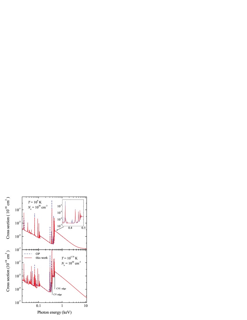
Figure 1.— Comparison of the carbon opacities published by Opacity Project (dashed curves) and computed in this work (solid curves) for two temperatures. The inset graph in the top panel shows a zoom into the region of the Lyman-like lines for the higher temperature. The ionization threshold energies of CVI and CV ions, 489 and 392 eV, respectively, are indicated by solid vertical lines in the bottom panel.

3. Basic properties of the models

Using the code described above, we have calculated an extended set of carbon NS atmosphere models. The models are computed for 9 values of surface gravity $\log g$, from 13.7 to 14.9 with a step of 0.15 , which cover most of realistic NS equations of state for a wide range of NS masses (Fig. 2). For every value of $\log g$, we computed 61 models with effective temperatures $T_{\rm eff}$ from 1 to 4 MK with a step of 0.05 MK.

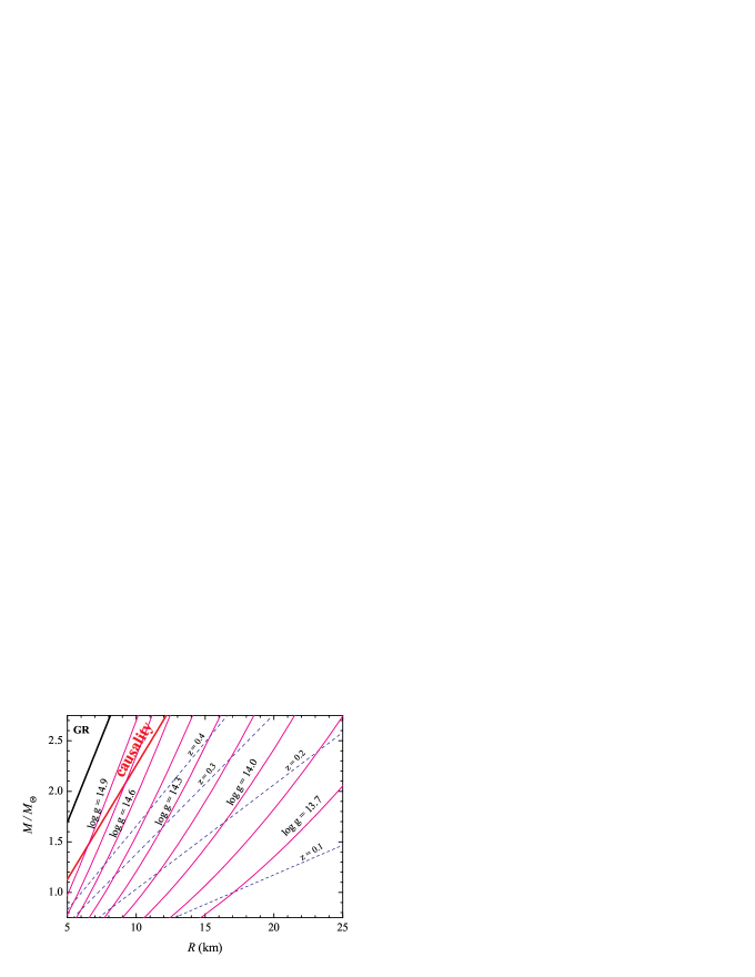
Figure 2.— Lines of constant $\log g$ values, for which our models were computed, in the $M$–$R$ plane. The limits of the forbidden regions in the upper-left corner of the plane are shown by thick lines. The dashed lines are the lines of constant gravitational redshift $z$.

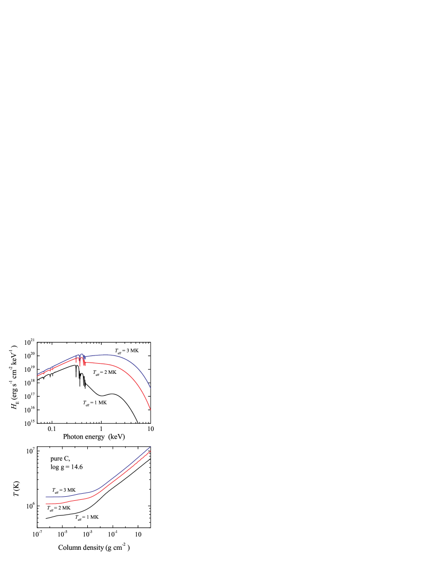
Figure 3.— Emergent spectra (top) and temperature structures (bottom) of pure carbon atmosphere models with $\log g=14.6$ and different effective temperatures.

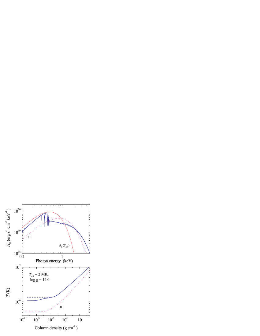
Figure 4.— Comparison of the emergent spectra (top) and temperature structures (bottom) of pure carbon atmosphere models computed with and without spectral lines (solid and dashed curves, respectively). The spectrum and the temperature structure of the pure hydrogen model are also shown (dotted curves). All the models have $T_{\rm eff}$ = 2 MK and $\log g$ = 14.0. The Planck function corresponding to 2 MK is shown in the top panel by the dash-dotted curve.

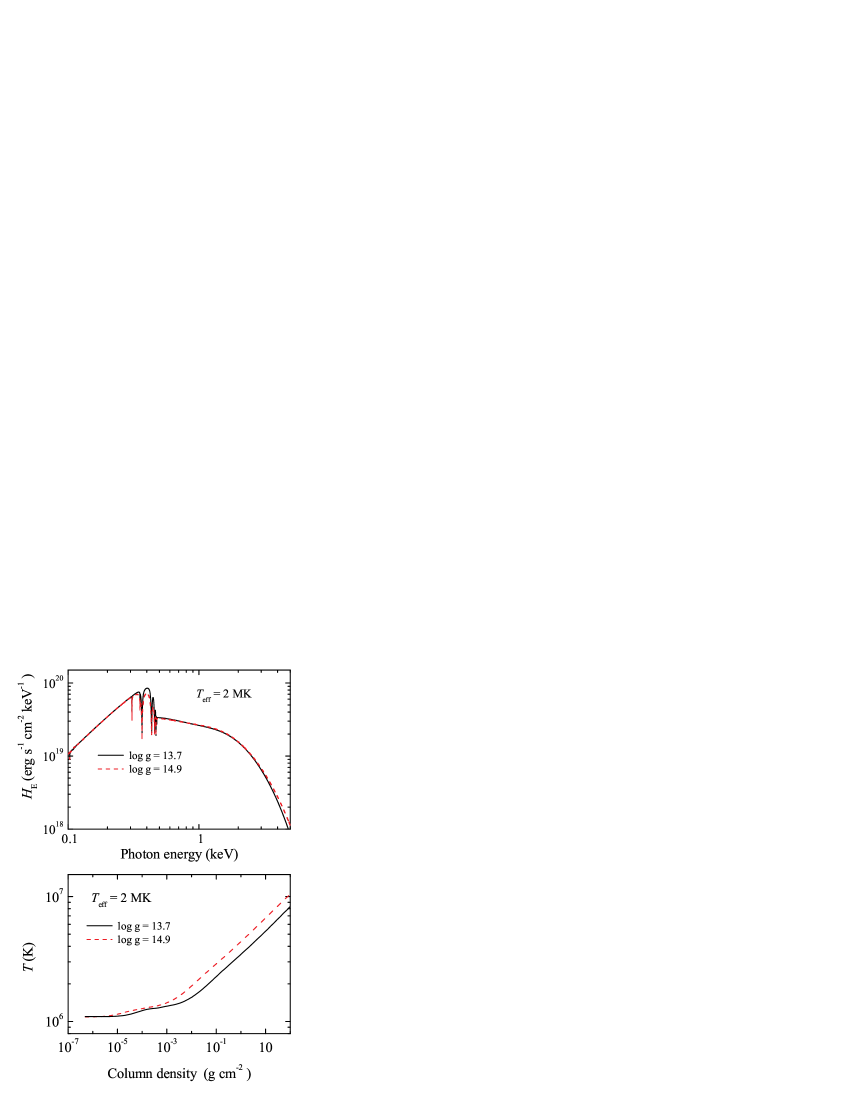
Figure 5.— Emergent spectra (top) and temperature structures (bottom) of pure carbon atmosphere models with $T_{\rm eff}$ = 2 MK and two extreme values of $\log g$, 14.9 and 13.7.

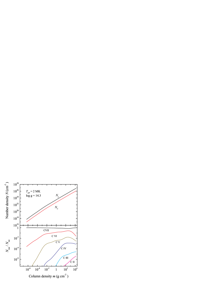
Figure 6.— Dependence of the number densities of electrons, $N_{e}$, and carbon ions, $N_{C}$ (top), and the ionization fractions (bottom) on the column depth for the carbon atmosphere model with $T_{\rm eff}=2$ MK and $\log g=14.3$.

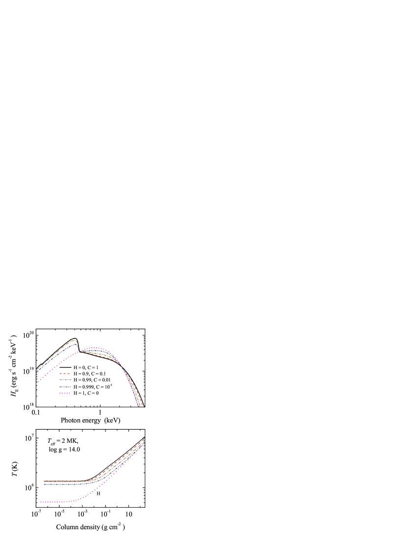
Figure 7.— Comparison of the emergent spectra (top) and temperature structures (bottom) for hydrogen+carbon models with different hydrogen/carbon fractions, from pure carbon to pure hydrogen. All the models correspond to $T_{\rm eff}$ = 2 MK and $\log g$ = 14.0 and were computed without taking into account spectral lines.

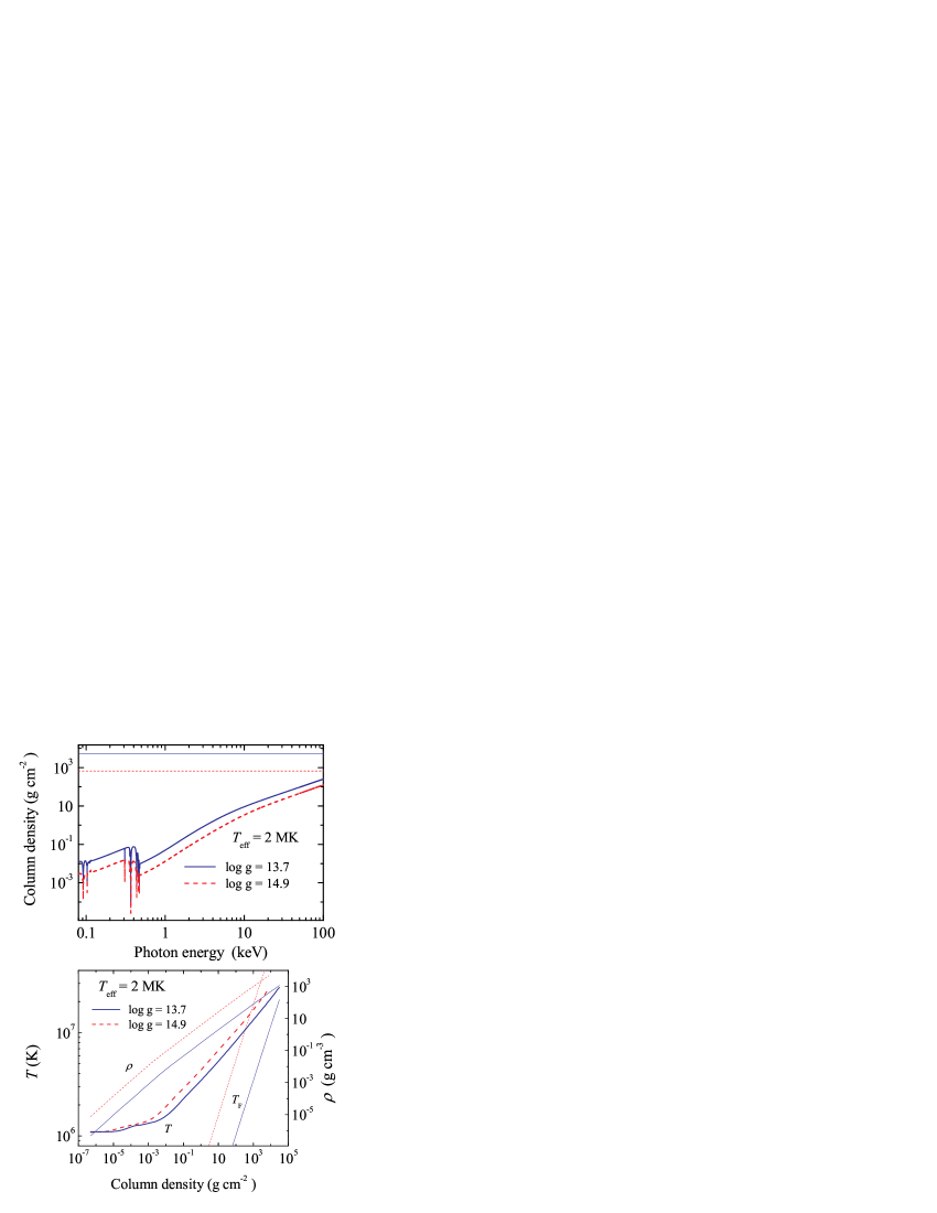
Figure 8.— Top: Comparison of the spectrum formation depths ($\tau_{\nu}^{\rm eff}$ = 1) with the depths where the Fermi temperature becomes larger than the model gas temperature (horizontal lines) for two pure carbon models: with $\log g$ = 13.7 (solid curves) and $\log g$ = 14.9 (dashed curves). Both models correspond to $T_{\rm eff}$ = 2 MK. Bottom: Temperature structures and the corresponding Fermi temperature distributions together with density distributions for the same models.

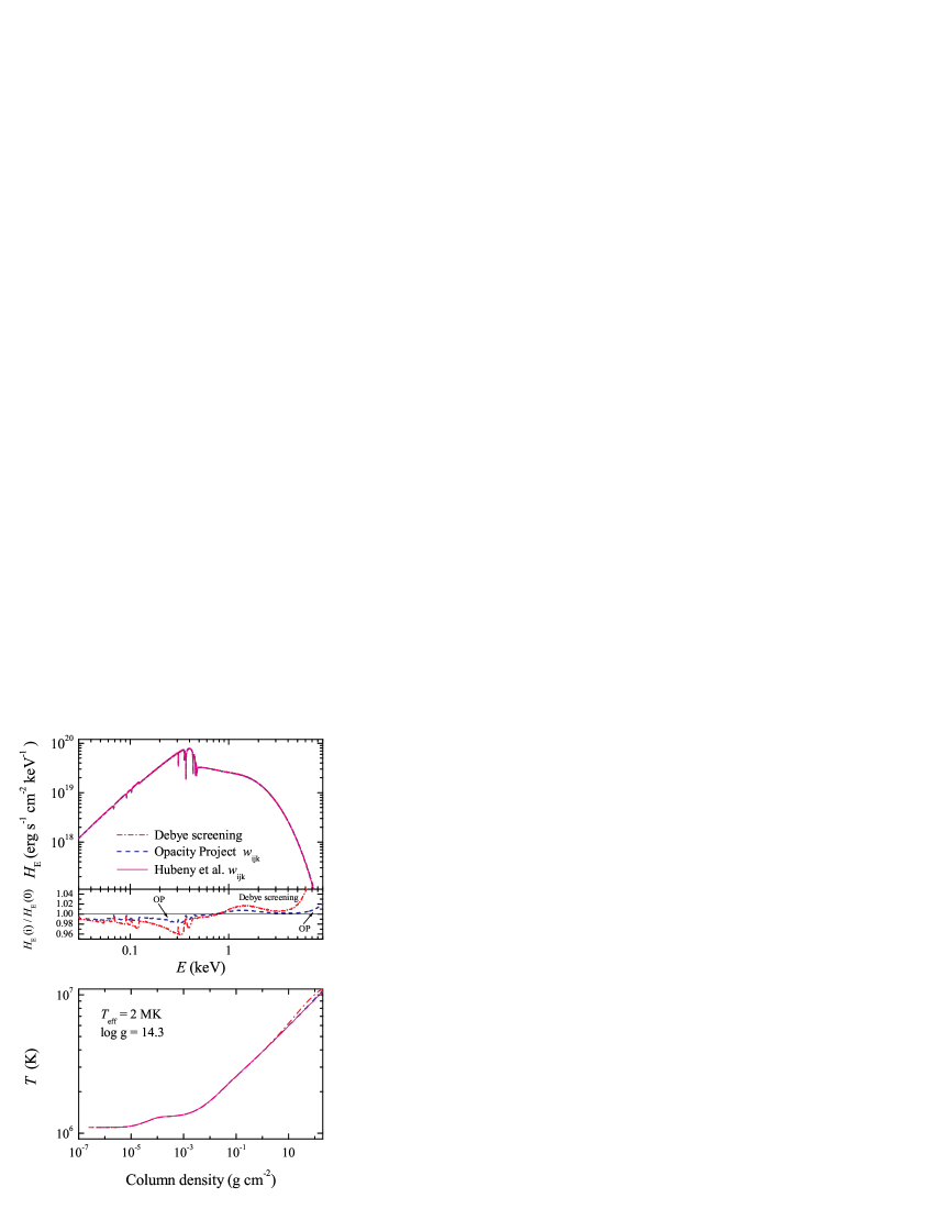
Figure 9.— Comparison of the emergent spectra (top) and temperature structures (bottom) of pure carbon atmospheres computed using three different approaches to account for pressure ionization (see text). The solid curves correspond to the computations using the approximation of Hubeny et al. (1994) adopted in our work, the dash-dotted curves correspond to the computations using a simple Debye screening, and the dashed curves indicate the models computed using the Opacity Project approximation. The ratios of the spectra of two latter models to the spectrum of the first one are shown in the sub-plot of the top panel.

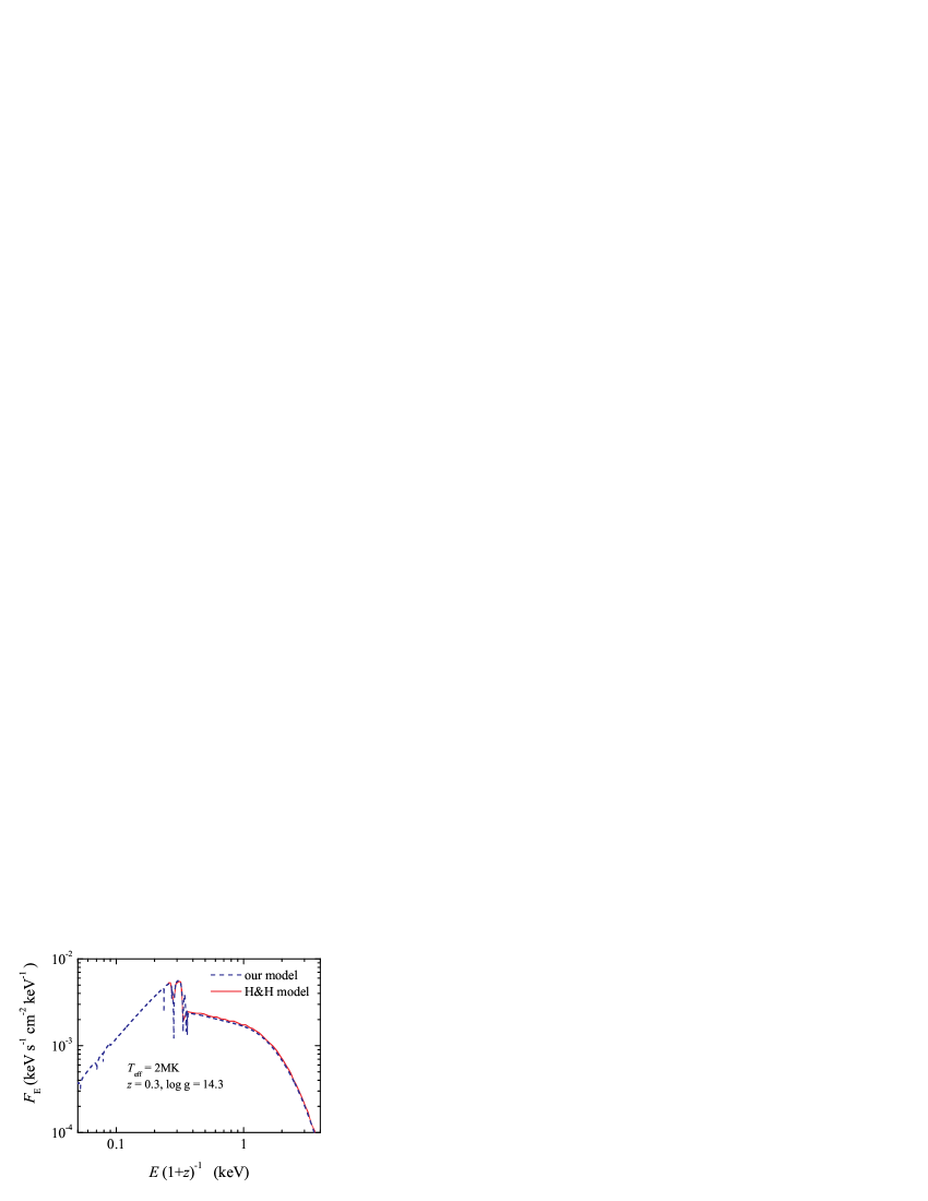
Figure 10.— Comparison of our redshifted model spectrum ($\log g$ = 14.3, $T_{\rm eff}$ = 2 MK, $z=0.3$, $d=3.4$ kpc, dashed curve), with the Ho & Heinke (2009) model spectrum (solid curve).

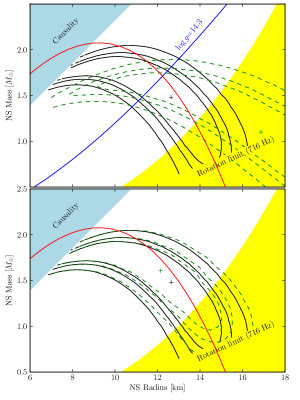
Figure 11.— Effect of gravitational acceleration and line-blanketing on the best-fit position and confidence contours (50%, 68%, and 90%) in the $M$–$R$ plane. The contours are obtained from fitting an XMM-Newton spectrum of the HESS J1731$-$347 CCO with three types of models, for a fixed distance $d=3.2$ kpc (Klochkov et al., 2013). The solid contours are obtained using the line-blanketed model atmosphere spectra with varying $\log g$ parameter. The dashed contours in the top panel are obtained from a subset of models with fixed $\log g=14.3$. The dashed contours in the bottom panel are obtained using model atmosphere spectra computed without account for spectral lines. The solid red curves correspond to $R_{\infty}=R(1+z)=16$ km, and the solid blue curve in the top panel corresponds to $\log g=14.3$.

Examples of the emergent spectra and temperature structures are shown in Figures 3 – 5, while Figure 6 shows the depth dependences of the density and ionization fractions. The absorption edges arising due to both CV and CVI ions are seen in the low temperature spectra. At higher temperatures, the number density of CV becomes so small that only the CVI edge is seen. The edges modify the spectra dramatically, causing strong deviations from the blackbody and hydrogen atmosphere specta of the same $T_{\rm eff}$ (see Fig. 4). Since the large opacity above the CVI ionization edge blocks the emergent flux at the maximum of the Planck function $B_{\rm E}(T_{\rm eff})$, this radiation flux has to be emitted at higher photon energies, where the atmosphere is more transparent. As a result, a nearly flat spectrum forms above the energy of the CVI ionization edge, $E>0.49$ keV, so that the carbon atmosphere spectrum is harder and has a lower spectral flux density than the hydrogen atmosphere spectrum at these energies. Also, the importance of taking into account the bound-bound transitions (spectral lines) is evident. The inclusion of the lines modifies the spectrum even at photon energies above the edge and leads to additional cooling of the upper atmosphere layers. The spectra of higher gravity models are slightly harder compared to the lower gravity models (see Fig. 5). We note that the absorption from the dissolved atomic levels is more important for the higher gravity models – see the continuum flux levels between the Ly$\alpha$- and Ly$\beta$-like spectral lines near $E\approx$ 0.4 keV.

In Figure 7, the emergent spectra and temperature structures of models with carbon-hydrogen mix are presented. It shows that the emergent spectra become very similar to the pure carbon atmosphere spectra already at a relatively low carbon abundance, $\sim 10\%$ of the hydrogen number density abundance.

Due to high densities in NS atmospheres, electron degeneracy may become important at a certain depth. We do not include this effect in our calculations. We can, however, evaluate its importance as follows. For a few models we have calculated the Fermi temperature $T_{\rm F}=E_{\rm F}/k$ corresponding to the electron number density $N_{\rm e}$: $E_{\rm F}=m_{\rm e}c^{2}(\sqrt{1+x^{2}}-1)$, where $x={p_{\rm F}}/{m_{\rm e}c}$, and $p_{\rm F}=h\left({3}N_{\rm e}/{8\pi}\right)^{1/3}.$ Electron degeneracy becomes important if the Fermi temperature is comparable to or larger than the gas temperature. For the computed models, the spectrum formation depths turn out to be considerably smaller than the depth where the Fermi temperature exceeds the electron gas temperature (see Fig. 8). The spectrum formation depth corresponds to column density $m$ where emergent photons are created or, equivalently, $\tau_{\nu}^{\rm eff}$ = 1.

Another effect of very high densities and/or low temperatures is a deviation of the equation of state from the ideal gas law due to the interactions between particles. Using calculations by Potekhin (1996), we have checked that such deviations are small in the layers where the emergent spectrum is formed, at the effective temperatures of our atmosphere models. Therefore, we conclude that neither the electron degeneracy nor the deviations from the ideal gas law affect the emergent spectra considerably (see also Suleimanov & Werner, 2007, in particular Fig. 6 of that paper).

We also investigated the accuracy of the method we used to account for the pressure ionization and level dissolution. For this purpose, we computed two additional model atmospheres where these effects are accounted for using different approaches. The first model is computed in the simplest approach, in which the ionization potential decrease is calculated as due to the Debye screening (see details in Kurucz, 1970). The second one is computed with the occupation probabilities $w_{ijk}$ calculated using the OP approximation (Seaton et al., 1994) instead of the Hubeny et al. (1994) approximation which we used. Here, $w_{ijk}$ is the probability that the bound level $i$ of the ionization stage $j$ of the chemical element $k$ is indeed bound. The value (1-$w_{ijk}$) gives the probability that this level is dissolved. It turns out that the models computed using these two other approaches give spectra and temperature structures very close to those of our model (see Fig. 9). This means that the differences in the pressure ionization and level dissolution descriptions may become important only at depths larger than the depth of the spectrum formation.

It is interesting to compare our model spectra with those published by Ho & Heinke (2009) using similar input parameters. The result of such a comparison, shown in Figure 10, demonstrates a good agreement.

4. Fitting NS spectra with the carbon atmosphere models

For fitting observed X-ray spectra with our models, we computed a suite of model spectra that can be directly used by the XSPEC package (XSPEC model carbatm). We converted the 549 computed model flux spectra to photon spectra in the energy range 0–20 keV, computing the numbers of photons in 1000 equal energy bins of 0.02 keV width. The fitting parameters of the model are the effective temperature $T_{\rm eff}$, the NS mass $M$ (in units of $M_{\odot}$) and radius $R$ (in units of km), and the normalization parameter $K$. For a given set of the fitting parameters, the surface gravity $g$ is calculated using Equation (1), the trial spectrum is computed using a linear interpolation between the nearest model spectra on the $T_{\rm eff}$–$\log g$ grid, and the boundaries of the energy bins and the number of photons in each bin are divided by $(1+z)$, defined by Equation (2). The normalization is defined as $K=A/d_{10}^{2}$, where $d_{10}$ is the distance to the source in units of 10 kpc, and $A$ characterizes the fraction of the NS surface which emits X-rays ($A=1$ if the radiation is produced by the entire NS surface). Obviously, $R$ and $d$ cannot be independently determined from a spectral fit because the observed flux is proportional to $R^{2}/d^{2}$. If the goal is to constrain the NS radius (and mass) for a source with a well-measured distance, and there are reasons to believe that the NS surface is uniformly heated ($A=1$), then $d$ (and $K$) can be fixed. If the distance is poorly known, then one can fix $R$ at a reasonable value (or set reasonable boundaries for varying $R$) and constrain $d$ (or $A^{-1/2}d$) from the fit.

The carbatm model has been tested by Klochkov et al. (2013) on the CCO in the HESS J1731$-$347 supernova remnant. Figure 4 of that paper shows confidence contours in the $M$–$R$ plane for two fixed distances and $A=1$. In Figure 11 of our paper we reproduce those contours for $d=3.2$ kpc (solid curves). In the top panel of Figure 11 we also show confidence contours (dashed curves) obtained for the same $d$ using the models with fixed $\log g$ = 14.3 (i.e., for any point in the $M$–$R$ plane we fit the observed spectrum using the subset of models with the fixed $\log g$ but applying the correct gravitational redshift). These contours differ substantially from the correct ones (except for the points close to the curve $\log g=14.3$), which demonstrates the effect of graviational acceleration and importance of using models with correct $\log g$ values. In the bottom panel of Figure 11 we show the confidence contours obtained from fitting the models in which bound-bound transitions (spectral lines) were neglected (dashed curves), which demonstrate the effect of line blanketing.

5. Discussion and Summary

In this work we have presented a detailed description of our carbon atmosphere models and demonstrated how the models can be applied to constrain the NS parameters. The models have already been used to fit the X-ray spectra of two CCOs, in the HESS J1731$-$347 and in Cas A supernova remnants. Although the inferred constraints on the NS mass and radius are consistent with many equations of state, the fits demonstrate that these NSs may be indeed covered by carbon atmospheres and radiate from the entire uniformly heated surface. These sources are good potential targets for further detailed investigations of the NS properties, including the NS cooling rates (see Heinke & Ho 2010 and Posselt et al. 2013), with the next generation of X-ray observatories.

In our work, we have thoroughly analyzed the accuracy of our assumptions for the carbon atmosphere computations. We have checked that our calculations of the carbon opacities and the number densities of carbon ions are consistent with the results of the Opacity Project. We found that the thermal conductivity of degenerate electrons, which determines the energy transport in the NS crust and deep atmosphere layers, becomes insignificant in the layers where the spectra are formed. We also showed that the model spectrum computed by Ho & Heinke (2009) is in close agreement with the one computed here.

There are, however, at least two physical effects which can impact on the accuracy of the presented model spectra. The first one is the assumption of LTE. We have computed the number densities of the carbon ions and the population of ion excited levels using the Saha-Boltzmann equations with the pressure ionization effects taken into account. In general, these quantities are determined by kinetic equilibrium between the rates of the radiative and collisional transitions that populate and de-populate ion states. Solving these kinetic equations constitutes the non-LTE approach (see e.g. Mihalas, 1978). A deviation from the LTE number density for H- and He-like carbon ions can modify the observed part of the emergent model spectra. The possible importance of this effect has been demonstrated for solar abundance NS model atmospheres (Rauch et al., 2008).

The second effect is the influence of a magnetic field. The investigated CCOs in Cas A and HESS J1731$-$347 do not show any evidence for a magnetic field, but even a relatively weak field strength ($B<10^{10}$ G) can affect the emergent model spectra via shifting the ion energy levels and ionization potentials, which changes the ion number densities and positions of the photoionization edges and spectral lines in emergent spectra (Pavlov & Potekhin, 1995; Potekhin & Pavlov, 1997; Mori & Ho, 2007; Engel et al., 2009) Moreover, even a weak magnetic field can broaden the carbon spectral lines due to Zeeman effect increasing the line-blanketing effect, which is important even without magnetic field.

All these effects can be important for measuring fundamental NS parameters, including masses and radii, and they will be investigated in future works.

References

- Abramowski et al. (2011) Abramowski, A., et al. 2011, A&A, 531, A81
- Acero et al. (2009) Acero, F., et al. 2009, in Proc. of the 31th ICRC 2009, Lodz (arXiv e-Print 0907.0642)
- Chandrasekhar (1946) Chandrasekhar, S. 1946, ApJ, 103, 351
- Changet al. (2010) Chang, P., Bildsten, L., & Arras, P. 2010, ApJ, 723, 719
- Cowley (1971) Cowley, R. L. 1971, The Observatory, 91, 139
- Dere et al. (1997) Dere, K. P., Landi, E., Mason, H. E., Monsignori Fossi, B. C., & Young, P. R. 1997, A&AS, 125, 149
- Engel et al. (2009) Engel, D., Klews, M., & Wunner, G. 2009, Comp. Phys. Commun., 180, 302
- Griem (1960) Griem, H. R. 1960, ApJ, 132, 883
- Gotthelf et al. (2013) Gotthelf, E. V., Halpern, J. P., & Alford, J. 2013, ApJ, 765, 58
- Halpern & Gotthelf (2010) Halpern, J. P., Gotthelf, E. V. 2010, ApJ, 709, 436
- Heinke et al. (2006) Heinke, C.O., Rybicki, G.B., Narayan, R., & Grindlay, J.E. 2006, ApJ, 644, 1090
- Ho & Heinke (2009) Ho, W. C. G., & Heinke, C. O. 2009, Nature, 462, 71
- Heinke & Ho (2010) Heinke, C. O., & Ho, W. C. G. 2010, ApJ, 719, L167
- Hubeny et al. (1994) Hubeny, I., Hummer, D., & Lanz, T. 1994, A&A, 282, 151
- Hummer & Mihalas (1988) Hummer, D. & Mihalas, D. 1988, ApJ, 331, 794
- Ibragimov et al. (2003) Ibragimov, A. A., Suleimanov, V. F., Vikhlinin, A., & Sakhibullin, N. A. 2003, Astronomy Reports, 47, 186
- Karzas & Latter (1961) Karzas, W. J. & Latter, R. 1961, ApJS, 6, 167
- Klochkov et al. (2013) Klochkov, D., Pühlhofer, G. Suleimanov, V., Simon, S., Werner, K., & Santangelo, A. 2013, A&A, 556, 41
- Kurucz (1993) Kurucz, R. 1993, ATLAS9 Stellar Atmosphere Programs and 2 km/s grid. Kurucz CD-ROM No. 13, Cambridge, Mass.: Smithsonian Astrophysical Observatory
- Kurucz (1970) Kurucz, R. L. 1970, SAO Special Report, 309
- Lattimer & Prakash (2007) Lattimer, J.M. & Prakash, M. 2007, Phys. Rep., 442, 109
- Mihalas (1978) Mihalas, D. 1978, Stellar atmospheres, 2nd edition (San Francisco, W. H. Freeman and Co.)
- Mori & Ho (2007) Mori, K. & Ho, W.C.G. 2007, MNRAS, 377, 905
- Olson & Kunasz (1987) Olson, G. L. & Kunasz, P. B. 1987, J. Quant. Spec. Radiat. Transf., 38, 325
- Pavlov & Potekhin (1995) Pavlov, G. G., & Potekhin, A. Y. 1995, ApJ, 450, 883
- Pavlov et al. (2000) Pavlov, G. G., Zavlin, V. E., Aschenbach, B., Trümper, J. & Sanwal, D. 2000, ApJ, 531, L35
- Pavlov et al. (2002a) Pavlov, G. G., Zavlin, V. E., & Sanwal, D. 2002a, in Proceedings of the 270 WE-Heraeus Seminar on Neutron Stars, Pulsars, and Supernova Remnants. MPE Report 278, ed. W. Becker, H. Lesch, & J. Trümper, Garching, MPE, p.273
- Pavlov et al. (2002b) Pavlov, G. G., Sanwal, D., Garmire, G. P., & Zavlin, V. E. 2002b, in Neutron Stars in Supernova Remnants, ASP Conf. Ser., vol. 271, ed. P. O. Slane & B. M. Gaensler (San Francisco: ASP), p.247
- Pavlov et al. (2004) Pavlov, G. G., Sanwal, D., & Teter, M. A. 2004, in IAU Symposium, Vol. 218, Young Neutron Stars and Their Environments, ed. F. Camilo & B. M. Gaensler, 239
- Pavlov & Luna (2009) Pavlov, G. G. & Luna, G. J. M. 2009, ApJ, 703, 910
- Posselt et al. (2013) Posselt, B., Pavlov, G. G., Suleimanov, V. F., & Kargaltsev, O. 2013, ApJ, accepted
- Potekhin (1996) Potekhin, A. Y. 1996, Phys. of Plasma, 3, 4156
- Potekhin & Pavlov (1997) Potekhin, A. Y., & Pavlov, G. G. 1997, ApJ, 483, 414
- Rauch et al. (2008) Rauch, T., Suleimanov, V., & Werner, K. 2008, A&A, 490, 1227
- Rogers & Iglesias (1992) Rogers, F. J., & Iglesias, C. A. 1992, ApJS, 79, 507
- Rosen (1968) Rosen, L. C. 1968, Ap&SS, 1, 372
- Seaton et al. (1994) Seaton, M. J., Yu Yan, Mihalas. D., & Pradhan, A. K. 1994, MNRAS, 266, 805
- Suleimanov & Werner (2007) Suleimanov, V. & Werner, K. 2007, A&A, 466, 661
- Sutherland (1998) Sutherland, R. S. 1998, MNRAS, 300, 321
- Verner & Yakovlev (1995) Verner, D. A. & Yakovlev, D. G. 1995, A&AS, 109, 125
- Verner et al. (1996) Verner, D. A., Ferland, G. J., Korista, K. T., & Yakovlev, D. G. 1996, ApJ, 465, 487
- Weisskopf et al. (2007) Weisskopf, M. C., Karovska, M., Pavlov, G. G., Zavlin, V. E., Clarke, T. 2007, Ap&SS, 308, 151
- Yakovlev & Pethick (2004) Yakovlev, D.G., & Pethick, C.J. 2004, ARA&A, 42, 169
- Zavlin et al. (1996) Zavlin, V.E., Pavlov, G.G. & Shibanov, Y.A. 1996, A&A, 315, 141
- Zavlinet al. (1998) Zavlin, V.E., Pavlov, G.G. & Trümper, J. 1998, A&A, 331, 821