Approximation Algorithms for Regret-Bounded Vehicle Routing and Applications to Distance-Constrained Vehicle Routing

Abstract

We consider vehicle-routing problems (VRPs) that incorporate the notion of regret of a client, which is a measure of the waiting time of a client relative to its shortest-path distance from the depot. Formally, we consider both the additive and multiplicative versions of, what we call, the regret-bounded vehicle routing problem (RVRP). In these problems, we are given an undirected complete graph $G=(\{r\}\cup V,E)$ on $n$ nodes with a distinguished root (depot) node $r$, edge costs $\{c_{uv}\}$ that form a metric, and a regret bound $R$. Given a path $P$ rooted at $r$ and a node $v\in P$, let $c_{P}(v)$ be the distance from $r$ to $v$ along $P$. The goal is to find the fewest number of paths rooted at $r$ that cover all the nodes so that for every node $v$ covered by (say) path $P$: (i) its additive regret $c_{P}(v)-c_{rv}$, with respect to $P$ is at most $R$ in additive-RVRP; or (ii) its multiplicative regret, $c_{P}(c)/c_{rv}$, with respect to $P$ is at most $R$ in multiplicative-RVRP.

Our main result is the first constant-factor approximation algorithm for additive-RVRP. This is a substantial improvement over the previous-best $O(\log n)$-approximation. Additive-RVRP turns out be a rather central vehicle-routing problem, whose study reveals insights into a variety of other regret-related problems as well as the classical distance-constrained VRP (DVRP), enabling us to obtain guarantees for these various problems by leveraging our algorithm for additive-RVRP and the underlying techniques. We obtain approximation ratios of $O\bigl{(}\log(\frac{R}{R-1})\bigr{)}$ for multiplicative-RVRP, and $O\bigl{(}\min\bigl{\{}\mathit{OPT},\frac{\log D}{\log\log D}\bigr{\}}\bigr{)}$ for DVRP with distance bound $D$ via reductions to additive-RVRP; the latter improves upon the previous-best approximation for DVRP.

A noteworthy aspect of our results is that they are obtained by devising rounding techniques for a natural configuration-style LP. This furthers our understanding of LP-relaxations for VRPs and enriches the toolkit of techniques that have been utilized for configuration LPs.

1 Introduction

Vehicle-routing problems (VRPs) constitute a broad class of combinatorial-optimization problems that find a wide range of applications and have been widely studied in the Operations Research and Computer Science communities (see, e.g., [24, 28, 37, 10, 6, 4, 30, 11] and the references therein). These problems are typically described as follows. There are one or more vehicles that start at some depot and provide service to an underlying set of of clients, and the goal is to design routes for the vehicles that visit the clients as quickly as possible. The most common way of formalizing the objective of minimizing client delays is to seek a route of minimum length, or equivalently, a route that minimizes the maximum client delay, which gives rise to (the path variant of) the celebrated traveling salesman problem (TSP). However, this objective does not differentiate between clients located at different distances from the depot, and a client closer to the depot may end up incurring a larger delay than a client that is further away, which can be considered a source of unfairness and hence, client dissatisfaction. Adopting a client-centric approach, we consider an alternate objective that addresses this unfairness and seeks to design routes that promote customer satisfaction.

Noting that the delay of a client is inevitably at least the shortest-path distance from the depot to the client location, following [35, 32], we seek to ensure that the regret of a client, which is a measure of its waiting time relative to its shortest-path distance from the depot, is bounded. More precisely, we consider the following genre of vehicle-routing problems. We are given an undirected complete graph $G=(\{r\}\cup V,E)$ on $n$ nodes with a distinguished root (depot) node $r$, and metric edge costs or distances $\{c_{uv}\}$. Given a path $P$ rooted at $r$ and a node $v\in P$, let $c_{P}(v)$ be the distance from $r$ to $v$ along $P$ (i.e., the length of the $r$-$v$ subpath of $P$). There are two natural ways of comparing $c_{P}(v)$ and $c_{rv}$ to define the regret of a node $v$ on path $P$. We define the additive regret of $v$ with respect to $P$ to be $c_{P}(v)-c_{rv}$, and the multiplicative regret of $v$ with respect to $P$ to be $c_{P}(v)/c_{rv}$. We are also given a regret bound $R$. Fixing a regret measure, a feasible solution is a collection of paths rooted at $r$ that cover all the nodes in $G$ such that the regret of every node with respect to the path covering it is at most $R$. Thus, a feasible solution to: (i) the additive-regret problem yields the satisfaction guarantee that every client $v$ is visited by time $c_{rv}+R$; and (ii) the multiplicative-regret problem ensures that every client $v$ is visited by time $c_{rv}\cdot R$. The goal is to find a feasible solution that uses the fewest number of paths. We refer to these two problems as additive-regret-bounded VRP (additive-RVRP) and multiplicative-regret-bounded VRP (multiplicative-RVRP) respectively.

Additive-RVRP has been sometimes referred to as the schoolbus problem in the literature [35, 32, 7]. However, this term is used to refer to an umbrella of vehicle-routing problems, some of which do not involve regret, so we use the more descriptive name of additive-RVRP. Both versions of RVRP are APX-hard via simple reductions from TSP and TSP-path (Theorem 7.1), so we focus on approximation algorithms.

Our results.

We undertake a systematic study of regret-related vehicle-routing problems from the perspective of approximation algorithms. As we illustrate below, additive-RVRP turns out to be the more fundamental of the above two problems and a rather useful problem to investigate, and our study yields insights and techniques that can be applied, often in a black-box fashion, to derive algorithms for various vehicle-routing problems, which include both regret-related problems, and classical problems such as distance-constrained vehicle routing. We therefore focus on additive regret; unless otherwise stated, regret refers to additive regret, and a regret-related problem refers to the problem under the additive-regret measure.

Our main result is the first constant-factor approximation algorithm for (additive) RVRP (Theorem 3.2). This is a substantial improvement over the previous-best $O(\log n)$-approximation ratio for RVRP obtained in [7] via the standard set-cover greedy algorithm and analysis.

Symmetric metrics					Asymmetric metrics
RVRP	$k$RVRP	Multiplicative-RVRP	Multiplicative-$k$RVRP	DVRP	RVRP	$k$RVRP
$\mathbf{31}$	$O(k^{2})$	$O\bigl{(}\log(\frac{R}{R-1})\bigr{)}$	$O(1)$	$O\bigl{(}\min\bigl{\{}\mathit{OPT},\frac{\log D}{\log\log D}\bigr{\}}\bigr{)}$	$O(\log n)$	$O(k^{2}\log n)$

Table 1: Summary of our results. Our main result, for RVRP, yields guarantees for other symmetric-metric problems.

A noteworthy aspect of our result is that we develop linear-programming (LP) based techniques for the problem. While LP-relaxations have been exploited with striking success in the design and analysis of approximation algorithms, our understanding of LP-relaxations for VRPs is quite limited (with TSP, and the minimum-latency problem to a lesser extent, being the exceptions), and this has been a stumbling block in the design of approximation algorithms for many of these problems. Notably, we develop LP-rounding techniques for a natural configuration-style LP-relaxation for RVRP, which is an example of the set-partitioning model for vehicle routing with time windows (see [37]). While it is not difficult to come up with such (approximately-solvable) configuration LPs for vehicle-routing problems, and they have been observed computationally to provide excellent lower bounds on the optimal value [13], there are few theoretical bounds on the effectiveness of these LPs. Moreover, the limited known guarantees (for general metrics) typically only establish logarithmic bounds [29, 7], which follow from the observation that the configuration LP can be viewed as a standard set-cover LP. In contrast, we exploit the structure of our configuration LP for RVRP using novel methods and prove a constant integrality gap for the relaxation, which serves to better justify the good empirical performance of these LPs. Although configuration LPs are often believed to be powerful, they have been leveraged only sporadically in the design of approximation algorithms; some notable exceptions are [25, 5, 36, 33, 14, 15]. Our work contributes to the toolkit of techniques that have been utilized for configuration LPs, and our techniques may find wider applicability.

We use our algorithm for additive-RVRP to obtain an $O\bigl{(}\log(\frac{R}{R-1})\bigr{)}$-approximation for multiplicative-RVRP with regret-bound $R$ (Theorem 4.2). Thus, we obtain a constant-factor approximation for any fixed $R$.

Interestingly, our algorithm for RVRP yields improved guarantees for (the path-variant of) the classical distance-constrained vehicle-routing problem (DVRP) [26, 28, 29, 30]—find the fewest number of rooted paths of length at most $D$ that cover all the nodes—via a reduction to RVRP. (DVRP usually refers to the version where we seek tours containing the root; [29] shows that the path- and tour-versions are within a factor of 2 in terms of approximability.) We obtain an $O\bigl{(}\frac{\log R_{\max}}{\log\log R_{\max}}\bigr{)}$-approximation for DVRP (Theorem 5.1), where $R_{\max}\leq D$ is the maximum regret of a node in an optimal solution, which improves upon the previous-best $O(\log D)$-guarantee for DVRP [29]. We believe that this reduction is of independent interest. Exploiting our LP-based guarantee for RVRP, we obtain the same integrality-gap bound for the natural configuration LP for DVRP. We also show that the integrality gap of the configuration LP is $O(\mathit{OPT}_{\text{LP}})$, where $\mathit{OPT}_{\text{LP}}$ is the optimal value of the LP. This is interesting because for the standard set-cover LP, there are $O(\log n)$-integrality-gap examples even when the optimal LP-value is a constant; although the DVRP-LP is also a set-cover LP, our result precludes such an integrality-gap construction for this LP and raises the enticing possibility that the additional structure in DVRP can be further exploited, perhaps by refining our methods, to derive improved guarantees.

We leverage our techniques to obtain guarantees for various variants and generalizations of RVRP (Section 6), including, most notably, (i) the variants where we fix the number $k$ of rooted paths (used to cover the nodes) and seek to minimize the maximum additive/multiplicative regret of a node, which we refer to as additive/multiplicative- $k$RVRP; and (ii) (additive) RVRP and $k$RVRP in asymmetric metrics.

We obtain an $O(k^{2})$-approximation for additive-$k$RVRP (Theorem 6.2), which is the first approximation guarantee for $k$RVRP. Previously, the only approximation results known for $k$RVRP were for the special cases where we have a tree metric [7] (note that the $O(\log n)$-distortion embedding of general metrics into tree metrics does not approximate regret), and when $k=1$ [6]. In particular, no approximation guarantees were known previously even when $k=2$; in contrast, we achieve a constant-factor approximation for any fixed $k$. Partially complementing this result, we show that the integrality gap of the configuration LP for $k$RVRP is $\Omega(k)$ (Theorem 7.4). Multiplicative-$k$RVRP turns out to be an easier problem, and the LP-rounding ideas in [9] yield an $O(1)$-approximation for this problem (Theorem 6.3).

For asymmetric metrics, we exploit the simple but key observation that regret can be captured via a suitable asymmetric metric that we call the regret metric $c^{\mathsf{reg}}$ (see Fact 2.1). This alternative view of regret yields surprising dividends, since we can directly plug in results for asymmetric metrics to obtain results for regret problems. In particular, results for $k$-person asymmetric $s$-$t$ TSP-path [17, 16] translate to results for asymmetric RVRP and $k$RVRP, and we achieve approximation ratios of $O(\log n)$ and $O(k^{2}\log n)$ respectively for these two problems. Although regret metrics form a strict subclass of asymmetric metrics, we uncover an interesting connection between the approximability of asymmetric RVRP and ATSP. We show that an $\alpha$-approximation for asymmetric RVRP implies a $2\alpha$-approximation for ATSP (Theorem 7.2); thus an $\omega(\log\log n)$-improvement to the approximation we achieve for asymmetric RVRP would improve the current best $O\bigl{(}\frac{\log n}{\log\log n}\bigr{)}$-approximation for ATSP [3].

Our techniques.

Our algorithm for additive-RVRP (see Section 3) is based on rounding a fractional solution to a natural configuration LP (P), where we have a variable for every path of regret at most $R$ and we enforce that every node is covered to an extent of 1 by such paths. Although this LP has an exponential number of variables, we can obtain a near-optimal solution $x^{*}$ by using an approximation algorithm for orienteering [6, 11] (see “Related work”) to provide an approximate separation oracle for the dual LP.

Let $k^{*}=\sum_{P}x^{*}_{P}$. To round $x^{*}$, we first observe that it suffices to obtain $O(k^{*})$ paths of total regret $O(k^{*}R)$ (see Lemma 2.2). At a high level, we would ideally like to ensure that directing the paths in the support of $x^{*}$ away from the root yields a directed acyclic graph $H$. If we have this, then by viewing $x^{*}$ as the path decomposition of a flow in $H$, and by the integrality property of flows, we can round $x^{*}$ to an integral flow that covers all the nodes, has value at most $\left\lceil k^{*}\right\rceil$, and whose cost in the regret metric is at most the $c^{\mathsf{reg}}$-cost of $x^{*}$, which is at most $k^{*}R$. This integral flow decomposes into a collection of $\left\lceil k^{*}\right\rceil$ paths that cover $V$ (since $H$ is acyclic), which yields the desired rounding.

Of course, in general, we will not be in this ideal situation. Our goal will be to identify a subset $W$ of “witness nodes” such that: (a) $x^{*}$ can be converted into a fractional solution that covers $W$ and has the above acyclicity-property without blowing up the $c^{\mathsf{reg}}$-cost by much; and (b) nodes in $V\setminus W$ can be attached to $W$ incurring only an $O(k^{*}R)$ cost. The new fractional solution can then be rounded to obtain integral paths that cover $W$, which in turn can be extended so that they cover $V$. In achieving this goal, we gain significant leverage from the fact that the configuration LP yields a collection of fractional simple paths that cover all the nodes, which is a stronger property than having a flow where every node has at least one unit of incoming flow. We build a forest $F$ of cost $O(k^{*}R)$ and select one node from each component of $F$ as a witness node; this immediately satisfies (b). The construction ensures that: first, every witness node $w$ has an associated collection of “witness paths” that cover it to a large extent, say, $\frac{1}{2}$; and second, for every path $P$, the witness nodes that use $P$ as a witness path have strictly increasing distances from the root $r$ and occur on $P$ in order of their distance from $r$. It follows that by shortcutting each path to only contain the witness nodes that use the path as a witness path, and blowing up the $x^{*}$ values by 2, we achieve property (a).

Our algorithms for multiplicative-RVRP and DVRP capitalize on the following insight. Suppose there exist $k$ paths covering a given set $S$ of nodes and incurring additive regret at most $\rho$ for these nodes. Then, for any $\epsilon>0$, one can use our algorithm for RVRP to find $O\bigl{(}\frac{k}{\epsilon}\bigr{)}$ paths covering $S$ such that the nodes in $S$ have additive regret at most $\epsilon\rho$ (Lemma 4.1). For multiplicative-RVRP with regret bound $R$, we apply this observation to every “ring” $V_{i}:=\{v:c_{rv}\in[2^{i-1},2^{i})\}$ to obtain $O(\mathit{OPT})$ paths covering $V_{i}$ such that the $V_{i}$-nodes face at most $(R-1)\cdot 2^{i-2}$ additive regret. This follows since the optimal solution covers $V_{i}$ inducing additive regret at most $(R-1)\cdot 2^{i}$ for these nodes. Concatenating the paths obtained for the $V_{i}$s whose indices are $O\bigl{(}\log(\frac{R}{R-1})\bigr{)}$ apart yields the $O\bigl{(}\log(\frac{R}{R-1})\bigr{)}$-approximation.

For DVRP, we build upon the above insight. Rather than fixing beforehand, as above, the regret bounds and the corresponding node-sets to cover via paths ensuring that regret bound, we use a dynamic-programming approach. Crucially, in the analysis, we bound the number of paths needed to cover a set of nodes with a given regret bound by suitably modifying the paths of a structured near-optimal solution $\mathcal{O}$. We argue that a specific choice (depending on $\mathcal{O}$) of regret bounds and node-sets yields an $O\bigl{(}\frac{\log R_{\max}}{\log\log R_{\max}}\bigr{)}$-approximation. In doing so, we argue that each choice of regret-bound is such that we make progress by decreasing substantially either the regret-bound or number of paths needed. Since our RVRP-algorithm is in fact LP-based, this also yields a bound on the integrality gap of the natural configuration LP for DVRP.

For the $O(\mathit{OPT}_{\text{LP}})$ integrality-gap result for DVRP, we show that one can partition the nodes so that for each part $S$, there is a distinct node $t_{S}$ such that the paths ending at $t_{S}$ cover the $S$-nodes to an extent of $\Omega\bigl{(}\frac{1}{\mathit{OPT}_{\text{LP}}}\bigr{)}$. Multiplying the LP-solution by $O(\mathit{OPT}_{\text{LP}})$ then yields a fractional solution that covers the $S$-nodes incurring regret at most $D-c_{rt_{S}}$, which we can round using our RVRP-algorithm.

Related work.

There is a wealth of literature on vehicle routing problems (see, e.g., [37]), and the survey [32] discusses a variety of problems under the umbrella of schoolbus-routing problems; we limit ourselves to the work that is relevant to our problems. The use of regret as a vehicle-routing objective seems to have been first considered in [35], who present various heuristics and empirical results.

Bock et al. [7] developed the first approximation algorithms for RVRP, but focus mainly on tree metrics, for which they achieve a 3-approximation. For general metrics, they observe that RVRP can be cast as a covering problem, and finding a minimum-density set is an orienteering problem [21, 6]: given node rewards, end points $s$, $t$, and a length bound $B$, find an $s$-$t$ path of length at most $B$ that gathers maximum total node-reward. Thus, the greedy set-cover algorithm combined with a suitable $O(1)$-approximation for orienteering [6, 11] immediately yields an $O(\ln n)$-approximation for RVRP. Previously, this was the best approximation algorithm for RVRP in general metrics. For $k$RVRP, no previous results were known for general metrics, even when $k=2$. (Note that we obtain a constant approximation for $k$RVRP for any fixed $k$.) [7] obtain a 12.5-approximation for $k$RVRP in tree metrics. When $k=1$, $k$RVRP becomes as a special case of the min-excess path problem introduced by [6], who devised a $(2+\epsilon)$-approximation for this problem.

To the best of our knowledge, multiplicative regret, and the asymmetric versions of RVRP and $k$RVRP have not been considered previously. Our algorithm for multiplicative-$k$RVRP uses the LP-based techniques developed by [9] for the minimum latency problem. The set-cover greedy algorithm can also be applied to asymmetric RVRP. This yields approximation ratios of $O\bigl{(}\frac{\log^{3}n}{\log\log n}\bigr{)}$ in polytime, and $O(\log^{2}n)$ in quasi-polytime using the $O\bigl{(}\frac{\log^{2}n}{\log\log n}\bigr{)}$- and $O(\log\mathit{OPT})$- approximation algorithms for directed orienteering in [31] and [12] respectively. Both factors are significantly worse than the $O(\log n)$-approximation that we obtain via an easy reduction to $k$ATSPP (find $k$ $s$-$t$ paths of minimum total cost that cover all nodes). Friggstad et al. [17] obtained the first results for $k$ATSPP which were later improved by [16] to an $O(k\log n)$-approximation and a bicriteria result that achieves $O(\log n)$-approximation using at most $2k$ paths.

Replacing the notion of client-regret in our problems with client-delay gives rise to some well-known vehicle-routing and TSP problems. The client-delay version of RVRP corresponds to (path-) DVRP. Nagarajan and Ravi [29] give an $O(\log\min\{D,n\})$-approximation for general metrics, and a 2-approximation for trees. Obtaining a constant-factor approximation for DVRP in general metrics has been a long-standing open problem. As noted earlier, regret can be captured by the asymmetric regret metric and thus RVRP is precisely (path-) DVRP in the regret metric. Thus, our work yields an $O(1)$-approximation for DVRP in this specific asymmetric metric. We find this to be quite interesting and surprising since one would normally expect that DVRP would become harder in an asymmetric metric.

The client-delay version of $k$RVRP yields the $k$TSP problem of finding $k$ rooted paths of minimum maximum cost that cover all nodes, which admits a constant-factor approximation via a reduction to TSP.

The orienteering problem plays a key role in vehicle-routing problems, including our algorithm for RVRP where it yields an approximate separation oracle for the dual LP. Blum et al. [6] obtained the first constant-factor approximation algorithm for orienteering, and the current best approximation is $2+\epsilon$ due to Chekuri et al. [11]. [31, 11] study (among other problems) directed orienteering and obtain approximation ratios of $O\bigl{(}\frac{\log^{2}n}{\log\log n}\bigr{)}$ and $O(\log^{2}\mathit{OPT})$ respectively. The backbone of all of these algorithms is the min-regret $K$-path problem (called the min-excess path problem in [6])—choose a min-regret path covering at least $K$ nodes—which captures $k$RVRP when $k=1$. [12] used a different approach and gave a quasi-polytime $O(\log\mathit{OPT})$-approximation for directed orienteering. Finally, Bansal et al. [4] and Chekuri et al. [11] consider orienteering with time windows, where nodes have time windows and we seek to maximize the number of nodes that are visited in their time windows, and its special case where nodes have deadlines, both of which generalize orienteering. They obtain polylogarithmic approximation ratios for these problems.

2 Preliminaries

Recall that an instance of RVRP is specified by a complete undirected graph $G=(\{r\}\cup V,E)$, where $r$ is a distinguished root node, with metric edge costs $\{c_{uv}\}$, and a regret-bound $R$. Let $n=|V|+1$. We call a path in $G$ rooted if it begins at $r$. Unless otherwise stated, we think of the nodes on $P$ as being ordered in increasing order of their distance along $P$ from $r$, and directing $P$ away from $r$ means that we direct each edge $(u,v)\in P$ from $u$ to $v$ if $u$ precedes $v$ (under this ordering). We use $D_{v}$ to denote $c_{rv}$ for all $v\in V\cup\{r\}$. For a set $S$ of edges, we sometimes use $c(S)$ to denote $\sum_{e\in S}c_{e}$. By scaling, and merging all nodes at distance 0 from each other, we may assume that $c_{uv}$ is a positive integer for all $u,v\in V\cup\{r\}$. Thus, $D_{v}\geq 1$ for all $v\in V$. Unless otherwise qualified, regret refers to additive regret in the sequel.

It will be convenient to assume that $R>0$: if $R=0$ then we can determine whether an edge $(u,v)$ lies on a shortest rooted path, and if so direct $(u,v)$ as $u\rightarrow v$ if $D_{v}=D_{u}+c_{uv}$, to obtain a directed acyclic graph (DAG) $H$. Our problem then reduces to finding the minimum number of directed rooted paths in $H$ to cover all the nodes, which can be solved efficiently using network-flow techniques.

The following equivalent way of viewing regret will be convenient. For every ordered pair of nodes $u,v\in V\cup\{r\}$, define the regret distance (with respect to $r$) to be $c^{\mathsf{reg}}_{uv}:=D_{u}+c_{uv}-D_{v}$.

Fact 2.1

(i) The regret distances $c^{\mathsf{reg}}_{uv}$ are nonnegative and satisfy the triangle inequality: $c^{\mathsf{reg}}_{uv}\leq c^{\mathsf{reg}}_{uw}+c^{\mathsf{reg}}_{wv}$ for all $u,v,w\in V\cup\{r\}$. Hence, $\{c^{\mathsf{reg}}_{uv}\}$ forms an asymmetric metric that we call the regret metric.

(ii) For a $u\leadsto v$ path $P$, we have $c^{\mathsf{reg}}(P):=\sum_{e\in P}c^{\mathsf{reg}}_{e}=D_{u}+c(P)-D_{v}$, and for a cycle $Z$, we have $c^{\mathsf{reg}}(Z)=c(Z)$. Properties (i) and (ii) hold even when the underlying $\{c_{uv}\}$ metric is asymmetric.

We infer from Fact 2.1 that if $P$ is a rooted path and $v\in P$, then the regret of $v$ with respect to $P$ is simply the $c^{\mathsf{reg}}$-distance to $v$ along $P$, which we denote by $c^{\mathsf{reg}}_{P}(v)$, and the regret of nodes on $P$ cannot decrease as one moves away from the root (since $c^{\mathsf{reg}}\geq 0$). We define the regret of $P$ to be the regret of the end-node of $P$, which by part (ii) of Fact 2.1 is given by $c^{\mathsf{reg}}(P)=\sum_{e\in P}c^{\mathsf{reg}}_{e}$.

Lemma 2.2 makes the key observation that one can always convert a collection of paths with average regret at most $\alpha R$ into one where every path has regret at most $R$ by blowing up the number of paths by an $(\alpha+1)$ factor, and hence, it suffices to obtain a near-optimal solution with average regret $O(R)$.

Lemma 2.2

Given rooted paths $P_{1},\ldots,P_{k}$ with total regret $\alpha kR$, we can efficiently find at most $(\alpha+1)\cdot k$ rooted paths, each regret at most $R$, that cover $\bigcup_{i=1}^{k}P_{i}$.

Proof.

Let $\alpha_{1}R,\ldots,\alpha_{k}R$ be the regrets of $P_{1},\ldots,P_{k}$ respectively. We show that for each path $P_{i}$, we can obtain $\max\{\left\lceil\alpha_{i}\right\rceil,1\}$ rooted paths of regret at most $R$ that cover the nodes of $P_{i}$. Applying this to each path $P_{i}$, we obtain at most $\sum_{i=1}^{k}(\alpha_{i}+1)=(\alpha+1)\cdot k$ rooted paths with regret at most $R$ that cover $\bigcup_{i=1}^{k}P_{i}$.

Fix a path $P_{i}$. If $\alpha_{i}\leq 1$, there is nothing to be done, so assume otherwise. The idea is to simply break $P_{i}$ at each point where the regret exceeds a multiple of $R$, and connect the starting point of each such segment directly to $r$. More formally, for $\ell=1,\ldots,\beta_{i}:=\left\lceil\alpha_{i}\right\rceil-1$, let $v_{\ell}$ be the first node on $P$ with $c^{\mathsf{reg}}_{P}(v)>\ell R$, and let $u_{\ell-1}$ be its (immediate) predecessor on $P$. Let $v_{0}=r$ and $u_{\beta_{i}}$ be the end point of $P_{i}$. We create the $\left\lceil\alpha_{i}\right\rceil$ paths given by $r,v_{\ell}\leadsto u_{\ell}$ for $\ell=0,\ldots,\beta_{i}$, which clearly together cover the nodes of $P_{i}$. The regret of each such path is $c^{\mathsf{reg}}_{rv_{\ell}}+c^{\mathsf{reg}}_{P}(u_{\ell})-c^{\mathsf{reg}}_{P}(v_{\ell})=c^{\mathsf{reg}}_{P}(u_{\ell})-c^{\mathsf{reg}}_{P}(v_{\ell})\leq(\ell+1)R-\ell R=R$, where the last inequality follows from the definitions of $v_{\ell}$, $v_{\ell+1}$ and $u_{\ell}$ (which precedes $v_{\ell+1}$). ∎

Approximation algorithms for symmetric TSP variants often exploit the fact that edges may be traversed in any direction, to convert a connected subgraph into an Eulerian tour while losing a factor of 2 in the cost. This does not work for RVRP since $c^{\mathsf{reg}}$ is an asymmetric metric. Instead, we exploit a key observation of Blum et al. [6], who identify portions of a rooted path $P$ whose total $c$-cost can be charged to $c^{\mathsf{reg}}(P)$.

Definition 2.3

Let $P$ be a rooted path ending at $w$. Consider an edge $(u,v)$ of $P$, where $u$ precedes $v$ on $P$. We call this a red edge of $P$ if there exist nodes $x$ and $y$ on the $r$-$u$ portion and $v$-$w$ portion of $P$ respectively such that $D_{x}\geq D_{y}$; otherwise, we call this a blue edge of $P$. For a node $x\in P$, let $\mathsf{red}(x,P)$ denote the maximal subpath $Q$ of $P$ containing $x$ consisting of only red edges (which might be the trivial path $\{x\}$).

We call a maximal blue/red subpath of a rooted path $P$ a blue/red interval of $P$. The blue and red intervals of $P$ correspond roughly to the type-1 and type-2 segments of $P$, as defined in [6]. Distinguishing the edges on $P$ as red or blue serves two main purposes. First, the total cost of the red edges is proportional to the regret of $P$ (Lemma 2.4). Second, if we shortcut $P$ so that it contains only one node from each red interval, then the resulting edges must all be distance increasing (Lemma 2.5). Consequently, if we perform this operation on a collection of paths and direct edges away from the root, then we obtain a DAG.

Lemma 2.4 (Blum et al. [6])

For any rooted path $P$, we have $\sum_{\text{$e$ red on $P$}}c_{e}\leq\frac{3}{2}c^{\mathsf{reg}}(P)$.

Proof.

Each red edge is contained in a “type-2 segment”, as defined in [6], and Corollary 3.2 in [6] proves that the total length of type-2 segments is at most $\frac{3}{2}\cdot c^{\mathsf{reg}}(P)$. ∎

Lemma 2.5

(i) Suppose $u,v$ are nodes on a rooted path $P$ such that $u$ precedes $v$ on $P$ and $\mathsf{red}(u,P)\neq\mathsf{red}(v,P)$, then $D_{u}<D_{v}$. (ii) Hence, if $P^{\prime}$ is obtained by shortcutting $P$ so that it contains at most one node from each red interval of $P$, then for every edge $(x,y)$ of $P^{\prime}$ with $x$ preceding $y$ on $P^{\prime}$, we have $D_{x}<D_{y}$.

Proof.

Since $u$ precedes $v$ on $P$ and $\mathsf{red}(u,P)\neq\mathsf{red}(v,P)$, there must be some edge $(a,b)\in P$ such that $(a,b)$ is blue on $P$, and $a$, $b$ lie on the $u$-$v$ portion of $P$ (note that it could be that $a=u$ and/or $b=v$). So if $D_{u}\geq D_{v}$ then $(a,b)$ would be classified as red. Part (ii) follows immediately from part (i). ∎

Orienteering.

Our algorithms are based on rounding the solution to an exponential-size LP-relaxation of the problem. A near-optimal solution to this LP can be obtained by solving the dual LP approximately. The separation oracle for the dual LP corresponds to a point-to-point orienteering problem, which is defined as follows. We are given an undirected complete graph with nonnegative node-rewards, edge lengths that form a metric, origin and destination nodes $s$, $t$, and a length bound $B$. The goal is to find an $s$-$t$ path $P$ of total length at most $B$ that gathers maximum total reward. In the rooted orienteering problem, we only specify the origin $s$, and a path rooted at $s$. Unless otherwise stated, we use orienteering to mean point-to-point orienteering. Clearly, an algorithm for orienteering can also be used for rooted orienteering. A related problem is the min-excess path (MEP) problem defined by [6], where we are given $s$, $t$, and a target reward $\Pi$, and we seek to find an $s$-$t$ path of minimum regret that gathers reward at least $\Pi$.

In the unweighted version of these problems, all node rewards are 0 or 1. Observe that the weighted versions of these problems can be reduced to their unweighted version in pseudopolynomial time by making co-located copies of a node. For orienteering, by suitably scaling and rounding the node-rewards, one can obtain a $\operatorname{\mathsf{poly}}\bigl{(}\text{input size},\frac{1}{\epsilon}\bigr{)}$-time reduction where we lose a $(1+\epsilon)$-factor in approximation. For MEP, this data rounding yields a bicriteria approximation where we obtain an $s$-$t$ path with reward at least $\Pi/(1+\epsilon)$. Both the unweighted and weighted versions of orienteering and MEP are NP-hard. The current best approximation factors for these problems are $(2+\epsilon)$ for orienteering due to Chekuri et al. [11], and $(2+\epsilon)$ for unweighted MEP due to Blum et al. [6], for any positive constant $\epsilon$.

3 An LP-rounding constant-factor approximation for (additive) RVRP

We consider the following configuration-style LP-relaxation for RVRP, which was also mentioned in [7]. Let $\mathcal{C}_{R}$ denote the collection of all rooted paths with regret at most $R$. We introduce a variable $x_{P}$ for each path $P\in\mathcal{C}_{R}$ to denote if path $P$ is chosen. Throughout, we use $P$ to index paths in $\mathcal{C}_{R}$.

$$\min\quad\sum_{P}x_{P}\qquad\text{s.t.}\qquad\sum_{P:v\in P}x_{P}\geq 1\quad\text{ for all }v\in V,\qquad x_{P}\geq 0\quad\text{ for all }P.$$ (P)

Let $\mathit{OPT}$ denote the optimal value of (P). Note that $\mathit{OPT}\geq 1$. It is easy to give a reduction from TSP showing that it is NP-complete to decide if there is a feasible solution that uses only 1 path; hence, it is NP-hard to achieve an approximation factor better than 2 (Theorem 7.1). Complementing this, we devise an algorithm for RVRP based on LP-rounding that achieves a constant approximation ratio (and thus yields a corresponding integrality-gap bound), which is a significant improvement over the previous-best $O(\log n)$-approximation ratio obtained by [7]. Although (P) has an exponential number of variables, one can obtain a near-optimal solution $x^{*}$ by solving the dual LP (which has an exponential number of constraints) to near-optimality, which can be achieved by using an approximation algorithm for orienteering to obtain an approximate separation oracle for the dual. We prove the following lemma in Section 8.

Lemma 3.1

We can use a $\gamma_{\mathsf{orient}}$-approximation algorithm for orienteering to efficiently compute a feasible solution $x^{*}$ to (P) of value at most $\gamma_{\mathsf{orient}}\cdot\mathit{OPT}$.

Let $k^{*}=\sum_{P}x^{*}_{P}$ (so $k^{*}\leq\gamma_{\mathsf{orient}}\cdot\mathit{OPT}$). Our goal is to round $x^{*}$ to a solution using at most $O(k^{*})$ paths that have average regret $O(R)$. We can then apply Lemma 2.2 to obtain $O(k^{*})$ paths, each having regret at most $R$, and thereby obtain an $O(1)$-approximate solution. We prove the following theorem.

Theorem 3.2

We can efficiently round $x^{*}$ to a solution using at most $(8+4\sqrt{3})k^{*}+1$ rooted paths. This yields $(8+4\sqrt{3})\gamma_{\mathsf{orient}}\mathit{OPT}+1\leq 30.86\cdot\mathit{OPT}$ rooted paths by taking $\gamma_{\mathsf{orient}}=2+\epsilon$ [11], and shows that the integrality gap of (P) is at most $9+4\sqrt{3}\leq 15.93$.

We first give an overview on the rounding procedure that obtains a slightly worse approximation ratio. We show in Section 3.1 how to refine this to obtain the guarantee stated above. Let ${\rm supp}(x^{*}):=\{P:x^{*}_{P}>0\}$ be the paths in the support of $x^{*}$. To gain some intuition, suppose first that it happens that when we direct every path $P\in{\rm supp}(x^{*})$ away from $r$, we obtain a directed graph $H$ that is acyclic. We can then set up a network-flow problem to find a minimum $c^{\mathsf{reg}}$-cost flow in $H$ of value at most $\left\lceil k^{*}\right\rceil$ such that every node has at least one unit of flow entering it. Since $x^{*}$ can be viewed as a path decomposition of a feasible flow of $c^{\mathsf{reg}}$-cost at most $k^{*}R$, by the integrality property of flows, there is an integral flow of $c^{\mathsf{reg}}$-cost at most $k^{*}R$. Since $H$ is acyclic, this flow may be decomposed into at most $\left\lceil k^{*}\right\rceil$ paths that cover all the nodes, and the average regret of this path collection is at most $R$, so we obtain the desired rounding.

Of course, in general $H$ will not be acyclic and rounding $x^{*}$ as above may yield an integral flow that does not decompose into a collection of only paths. So we seek to identify a subset $W\subseteq V$ of “witness” nodes and a collection of $O(k^{*})$ fractional paths from $\mathcal{C}_{R}$ covering $W$ such that: (a) directing each path in this collection away from $r$ yields a DAG; and (b) given any collection of integral paths covering $W$, one can graft the nodes of $V\setminus W$ into these paths (to obtain new paths covering $V$) incurring an additional $c^{\mathsf{reg}}$-cost of $O(k^{*}R)$. Property (a) allows one to use the aforementioned network-flow argument to obtain $O(k^{*})$ paths covering $W$ with total regret $O(k^{*}R)$, and property (b) enables one to modify this to obtain $O(k^{*})$ (integral) paths covering $V$ while keeping the total regret to $O(k^{*}R)$ (so that one can then apply Lemma 2.2).

To obtain $W$, we carefully construct a forest $F$ of cost $O(k^{*}R)$ (step A1 below) with the property that for every component $Z$ of $F$, we can associate a single node $w\in Z$, which we include in $W$, such that there is a total $x^{*}$-weight of at least $0.5$ in paths $P$ containing $w$ for which $\mathsf{red}(w,P)\subseteq Z$. Notably, we achieve this in a rather clean and simple way by defining a downwards-monotone cut-requirement function based on the fractional solution $x^{*}$ that encodes the above requirement, an idea that we believe has wider applicability, especially for network-design problems.

Once we have such a forest, property (b) holds by construction since the total cost of $F$ is $O(k^{*}R)$ (Lemma 3.3). Moreover (step A2), if we shortcut each path $P\in{\rm supp}(x^{*})$ so that it only contains nodes $w\in W$ for which $\mathsf{red}(w,P)$ is contained in some component of $F$, then the resulting paths cover each node in $W$ to an extent of at least $0.5$ and satisfy the conditions of part (ii) of Lemma 2.5 (see Lemma 3.4). So by doubling the fractional values of the resulting paths, we obtain a fractional-path collection satisfying property (a). Hence, we can obtain $O(k^{*})$ integral paths covering $W$ (step A3) and attach the nodes of $V\setminus W$ to these paths (step A4) while ensuring that the total regret remains $O(k^{*}R)$ (Lemma 3.5), and then apply Lemma 2.2. We prove in Theorem 3.6 that the resulting solution uses at most $16k^{*}+1\leq 16\gamma_{\mathsf{orient}}\cdot\mathit{OPT}+1$ paths. In Section 3.1, we show how to obtain the improved guarantee stated in Theorem 3.2 by fine-tuning the threshold used to form the forest $F$. We now describe the algorithm in detail and proceed to analyze it.

Algorithm 1

 

Input: A fractional solution $x^{*}$ to (P) obtained via Lemma 3.1; $k^{*}=\sum_{P}x^{*}_{P}$.

Output: $O(k^{*})$ paths, each having regret at most $R$, covering all the nodes.

• Finding a low-cost forest $F$.  For a subset $S\subseteq V\cup\{r\}$ and a node $v$, define $\tau(v,S):=\sum_{P:\mathsf{red}(v,P)\subseteq S}x^{*}_{P}$; define $f(S)=1$ if $\tau(v,S)<\frac{1}{2}$ for all $v\in S$, and 0 otherwise. Note that $f$ is a downwards-monotone cut-requirement function: if $\emptyset\neq A\subseteq B$ then $f(A)\geq f(B)$. We call a set $S$ with $f(S)=1$, an active set.

  • Use the 2-approximation algorithm for $\{0,1\}$ downwards-monotone functions in [19] to obtain a forest $F$ such that $|\delta(S)\cap F|\geq f(S)$ for every set $S\subseteq V\cup\{r\}$.

  • For every component $Z$ of $F$ with $r\notin Z$, choose a node $w\in Z$ such that $\tau(w,Z)\geq\frac{1}{2}$ (which exists since $f(Z)=0$). Call $w$ the witness node for $Z$, and denote $Z$ by $Z_{w}$. Obtain a tour $h(Z)$ traversing all nodes of $Z$ by doubling the edges of $Z$ and shortcutting. Let $W\subseteq V$ be the set of all witness nodes.

• Obtaining a fractional acyclic flow covering $W$. 

  • For every path $P\in{\rm supp}(x^{*})$ we do the following. Let $P_{W}\subseteq P\cap W$ be the set of witness nodes $w\in P$ such that $\mathsf{red}(w,P)$ is contained in $Z_{w}$. We shortcut $P$ past the nodes in $P\setminus(P_{W}\cup\{r\})$ to obtain a rooted path $\phi(P)$ spanning the nodes in $P_{W}$. Note that shortcutting does not increase the $c^{\mathsf{reg}}$-cost. Let $\mathcal{C}^{\prime}\subseteq\mathcal{C}_{R}=\{\phi(P):P\in{\rm supp}(x^{*}),\phi(P)\neq\{r\}\}$ denote this new collection of non-trivial paths.

  • Let $H=(\{r\}\cup V,A_{H})$ be the directed graph obtained by directing each path in $\mathcal{C}^{\prime}$ away from $r$. Let $z=(z_{a})_{a\in A_{H}}$ be the flow that sends $\sum_{P:\phi(P)=P^{\prime}}x^{*}_{P}$ flow along each path $P^{\prime}\in\mathcal{C}^{\prime}$. We prove in Lemma 3.4 that $H$ is acyclic, and that $z^{\mathrm{in}}(w):=\sum_{a\in\delta_{H}^{\mathrm{in}}(w)}z_{a}\geq\frac{1}{2}$ for every $w\in W$.

• Use the integrality property of flows to round $2z$ to an integer flow $\hat{z}$ of no greater $c^{\mathsf{reg}}$-cost and value $k\leq\left\lceil 2k^{*}\right\rceil$ such that $\hat{z}^{\mathrm{in}}(w)\geq 1$ for every $w\in W$. Since $H$ is acyclic, we may decompose $\hat{z}$ into $k$ rooted paths $\hat{P}_{1},\ldots,\hat{P}_{k}$ so that (possibly after some shortcutting) every node of $W$ lies on exactly one $\hat{P}_{i}$ path.

• Grafting in the nodes of $V\setminus W$.  If there is a component $Z$ of $F$ containing $r$, we pick an arbitrary path, say $\hat{P}_{1}$, and modify $\hat{P}_{1}$ by traversing $h(Z)$ first and then visiting the nodes of $\hat{P}_{1}\setminus\{r\}$ (in the same order as $\hat{P}_{i}$). Next, for every path $\hat{P}_{i},\ i=1,\ldots,k$, we walk along $\hat{P}_{i}$ and each time we visit a new node $w\in W$ on $\hat{P}_{i}$ we traverse $h(Z_{w})$ before moving on to the next node on $\hat{P}_{i}$. Let $\tilde{P}_{i}$ denote the resulting new path.

• Apply Lemma 2.2 to $\tilde{P}_{1},\ldots,\tilde{P}_{k}$ to obtain the final set of paths (having maximum regret $R$).

 

Analysis.

Let $\mathcal{S}(F)$ denote the set of components of $F$. Note that $V\subseteq\bigcup_{Z\in\mathcal{S}(F)}Z$.

Lemma 3.3

The forest $F$ computed in step A1 has cost at most $6\cdot k^{*}\cdot R$. Thus, $\sum_{Z\in\mathcal{S}(F)}c(h(Z))\leq 12k^{*}R$.

Proof.

Consider the following LP for covering the cuts $\delta(S)$ corresponding to active sets $S$.

$$\min\quad\sum_{e}c_{e}z_{e}\qquad\text{s.t.}\qquad z(\delta(S))\geq 1\quad\forall\emptyset\subsetneq S\subseteq V\cup\{r\},\qquad z\geq 0.$$ (C-P)

Define $z$ by setting $z_{e}=\sum_{P:e\text{ is red on }P}2\cdot x^{*}_{P}$ for all $e$. This is a feasible solution to (C-P) since for every active set $S$ and every node $v\in S$, we have that

$$\frac{1}{2}<1-\tau(v,S)\leq\sum_{P:\mathsf{red}(v,P)\not\subseteq S}x^{*}_{P}\leq\sum_{e\in\delta(S)}\Bigl{(}\sum_{P:e\in\mathsf{red}(v,P)}x^{*}_{P}\Bigr{)}\leq z(\delta(S))/2.$$

Also, $\sum_{e}c_{e}z_{e}=2\sum_{P}x^{*}_{P}\bigl{(}\sum_{\text{$e$ red on $P$}}c_{e}\bigr{)}\leq 3\sum_{P}c^{\mathsf{reg}}(P)x^{*}_{P}\leq 3k^{*}R$. The penultimate inequality follows from Lemma 2.4, and the last inequality follows because ${\rm supp}(x^{*})\subseteq\mathcal{C}_{R}$ and $\sum_{P}x^{*}_{P}=k^{*}$. The 2-approximation algorithm of [19] then guarantees that $c(F)\leq 2\cdot\mathit{OPT}_{\eqref{cutlp}}\leq 6k^{*}R$, Since $c(h(Z))\leq 2c(Z)$ for component $Z$ of $F$, we have $\sum_{Z\in\mathcal{S}(F)}c(h(Z))\leq 12k^{*}R$. ∎

Lemma 3.4

(i) For every path $P\in\mathcal{C}_{R}$, every red interval of $P$ contains at most one node of $P_{W}$. Therefore, $\phi(P)$ visits nodes $v$ in strictly increasing order of $D_{v}$; (ii) $\sum_{P:w\in\phi(P)}x^{*}_{P}\geq\frac{1}{2}$ for every $w\in W$; (iii) Hence, the digraph $H$ constructed in step A2 is acyclic, and $z^{\mathrm{in}}(w)\geq\frac{1}{2}$ for every $w\in W$.

Proof.

Part (iii) follows immediately from parts (i) and (ii). For part (i), recall that $P_{W}=\{w\in P\cap W:\mathsf{red}(w,P)\subseteq Z_{w}\}$. If there are two nodes $u$, $w$ of $P_{W}$ contained in some red interval of $P$ then $Z_{u}\cap Z_{w}\neq\emptyset$, but this contradicts the fact that we add at most one node to $W$ from each component of $F$. It follows that $\phi(P)$ contains at most one node from each red interval of $P$, and by Lemma 2.5, we have that $\phi(P)$ visits nodes $v$ in strictly increasing order of distance $D_{v}$. For part (ii), we note that for a node $w\in W$, by definition, we have that $w\in\phi(P)$ iff $\mathsf{red}(w,P)\subseteq Z_{w}$. So $\sum_{P:w\in\phi(P)}x^{*}_{P}=\sum_{P:\mathsf{red}(w,P)\subseteq Z_{w}}x^{*}_{P}=\tau(w,Z_{w})\geq\frac{1}{2}$, where the last inequality follows from the definition of $Z_{w}$. ∎

Lemma 3.5

The total regret of the paths $\tilde{P}_{1},\ldots,\tilde{P}_{k}$ obtained in step A4 is at most $14\cdot k^{*}\cdot R$.

Proof.

Let $Z_{r}$ denote the component of $Z$ containing $r$; let $Z_{r}=\emptyset$ and $h(Z_{r})=0$ if there is no such component. The regret of path $\tilde{P}_{1}$ is $c^{\mathsf{reg}}(\hat{P}_{1})+\sum_{w\in\hat{P}_{1}}c^{\mathsf{reg}}\bigl{(}h(Z_{w})\bigr{)}$ and the regret of $\tilde{P}_{i}$ for $i\neq 1$ is $c^{\mathsf{reg}}(\hat{P}_{i})+\sum_{w\in\hat{P}_{i}:w\neq r}c^{\mathsf{reg}}\bigl{(}h(Z_{w})\bigr{)}$.

The paths $\hat{P}_{1},\ldots,\hat{P}_{k}$ obtained after step A3 have $c^{\mathsf{reg}}$-cost at most the $c^{\mathsf{reg}}$-cost of $2z$, which is $2\sum_{P^{\prime}\in\mathcal{C}^{\prime}}c^{\mathsf{reg}}(P^{\prime})\sum_{P:\phi(P)=P^{\prime}}x^{*}_{P}\leq\sum_{P}c^{\mathsf{reg}}(P)x^{*}_{P}\leq 2k^{*}R$. Since the $c^{\mathsf{reg}}$- and $c$-costs of a cycle are identical (by Fact 2.1), the total regret of $\tilde{P}_{1},\ldots,\tilde{P}_{k}$ is at most $\sum_{i=1}^{k}c^{\mathsf{reg}}(\hat{P}_{i})+\sum_{Z\in\mathcal{S}(F)}c\bigl{(}h(Z)\bigr{)}\leq 2k^{*}R+12k^{*}R=14k^{*}R$, where we use Lemma 3.3 for the last inequality. ∎

Theorem 3.6

Algorithm 1 returns a feasible solution with at most $16k^{*}+1\leq 16\gamma_{\mathsf{orient}}\cdot\mathit{OPT}+1$ paths.

Proof.

Applying Lemma 2.2 to the paths $\tilde{P}_{1},\ldots,\tilde{P}_{k}$, which have total regret at most $14k^{*}R$ (by Lemma 3.5), we obtain a collection of $k^{\prime}$ rooted paths of maximum regret $R$ whose union covers all nodes, where $k^{\prime}\leq\bigl{(}\frac{14k^{*}}{k}+1\bigr{)}k\leq 14k^{*}+k\leq 14k^{*}+\left\lceil 2k^{*}\right\rceil\leq 16k^{*}+1$. ∎

3.1 Improvement to the guarantee stated in Theorem 3.2

We now describe the improvement that yields Theorem 3.2. Let $\delta\in(0,1)$ be a parameter that we will fix later. The only change is that we now define the cut-requirement function in step A1 as $f(S)=1$ if $\tau(v,S)<\delta$ for all $v\in S$, and 0 otherwise. This results in a corresponding change to the integer flow $\hat{z}$ obtained in step A2.

Mimicking the proof of Lemma 3.3, we see that setting $z_{e}=\sum_{P:\text{$e$ is red on $P$}}x^{*}_{P}/(1-\delta)$ yields a feasible solution to (C-P), and therefore we have, $c(F)\leq\frac{3}{1-\delta}\cdot k^{*}R$, and $\sum_{Z\in\mathcal{S}(F)}c(h(Z))\leq\frac{6}{1-\delta}\cdot k^{*}R$. Step A2 is unchanged, but parts (ii) and (iii) of Lemma 3.4 need to be suitably modified: we now have that the flow $z$ satisfies $z^{\mathrm{in}}(w)\geq\delta$ for every $w\in W$. Correspondingly, we round $z/\delta$ to an integer flow in step A3, and obtain at most $\left\lceil k^{*}/\delta\right\rceil$ paths. Proceeding as in the proof of Lemma 3.5, we infer that the total regret of the paths obtained after grafting in the nodes of $V\setminus W$ is at most $\bigl{(}\frac{1}{\delta}+\frac{6}{1-\delta}\bigr{)}k^{*}R$.

Applying Lemma 2.2, this yields at most $\bigl{(}\frac{1}{\delta}+\frac{6}{1-\delta}\bigr{)}k^{*}+\left\lceil\frac{k^{*}}{\delta}\right\rceil\leq\bigl{(}\frac{2}{\delta}+\frac{6}{1-\delta}\bigr{)}k^{*}+1$ paths having regret at most $R$. Taking $\delta=\frac{\sqrt{3}-1}{2}$ to minimize the coefficient of $k^{*}$, we obtain the guarantee stated in Theorem 3.2.

4 Multiplicative-RVRP

Recall that in multiplicative-RVRP, we are given a regret-bound $R$, and we want to find the minimum number of paths covering all nodes so that each node $v$ is visited by time $R\cdot D_{v}$. When $R=1$, the problem can be solved in polytime (as this is simply additive-RVRP with regret-bound 0), so we assume that $R>1$. We show that multiplicative-RVRP reduces to RVRP incurring an $O\bigl{(}\log(\frac{R}{R-1}\bigr{)}$-factor loss. The following observation, which falls out of Lemma 2.2 will be quite useful.

Lemma 4.1

Let $\gamma_{\mathsf{RVRP}}$ be the approximation ratio of our RVRP-algorithm. Suppose there are $k$ paths covering a given set $S$ of nodes ensuring that every node in $S$ has additive regret at most $\rho$. For any $\epsilon>0$, one can efficiently obtain at most $\left\lfloor\gamma_{\mathsf{RVRP}}k\left\lceil\frac{1}{\epsilon}\right\rceil\right\rfloor$ paths covering $S$ such that each node in $S$ has regret at most $\epsilon\rho$.

Proof.

We shortcut the $k$ paths so that they only contain the nodes in $S$. The regret of each of these $k$ paths is at most $\rho$, so as in Lemma 2.2, we may break up each path into at most $\left\lceil\frac{1}{\epsilon}\right\rceil$ paths of regret at most $\epsilon\rho$. This creates at most $k\left\lceil\frac{1}{\epsilon}\right\rceil$ paths of regret at most $\epsilon\rho$ that cover $S$. So by using our algorithm for RVRP with the node-set $r\cup S$ and regret-bound $\epsilon\rho$, we obtain $\gamma_{\mathsf{RVRP}}k\left\lceil\frac{1}{\epsilon}\right\rceil$ paths of regret at most $\epsilon\rho$ covering $S$. Since the number of paths is an integer, we actually have $\left\lfloor\gamma_{\mathsf{RVRP}}k\left\lceil\frac{1}{\epsilon}\right\rceil\right\rfloor$ paths. ∎

Theorem 4.2

Multiplicative-RVRP can be reduced to additive-RVRP incurring an $O\bigl{(}\log(\frac{R}{R-1})\bigr{)}$-factor loss. This yields an $O\bigl{(}\log(\frac{R}{R-1})\bigr{)}$-approximation for multiplicative-RVRP.

Proof.

Let $R=1+\delta$. For $i\geq 1$, define $V_{i}=\{v:2^{i-1}\leq D_{v}<2^{i}\}$. Note that the $V_{i}$s partition the non-root nodes. Let $O^{*}$ denote the optimal value of the multiplicative-RVRP instance. We apply Lemma 4.1 with $\epsilon=\frac{1}{4}$ to the $V_{i}$s: for each $V_{i}$, there are $O^{*}$ paths covering $V_{i}$ such that each node in $V_{i}$ has regret at most $\delta\cdot 2^{i}$, so we obtain at most $N=\left\lfloor 4\gamma_{\mathsf{RVRP}}O^{*}\right\rfloor=O(O^{*})$ paths covering $V_{i}$ such that each node in $V_{i}$ has regret at most $\delta\cdot 2^{i-2}$. Pad these with the trivial path $\{r\}$ if needed, to obtain exactly $N$ paths $P^{i}_{1},\ldots,P^{i}_{N}$.

Let $M=\left\lceil\log_{2}\bigr{(}3+\frac{8}{\delta}\bigr{)}\right\rceil=O\bigl{(}\log_{2}(\frac{R}{R-1})\bigr{)}$. Now for every index $i=1,2,\ldots,M$ and every $j=1,\ldots,N$, we concatenate the paths $P^{i}_{j},P^{i+M}_{j},P^{i+2M}_{j},\ldots$ by moving from the end-node of $P^{i+aM}_{j}$ to $r$ before following $P^{i+(a+1)M}_{j}$ for each $a\geq 0$. This yields $MN$ paths that together cover all nodes.

To finish the proof, we show that every node $v$ is visited by time $R\cdot D_{v}$. Suppose $v\in V_{i+aM}$ and is covered by path $P^{i+aM}_{j}$. It’s visiting time is then at most $c_{P^{i+aM}_{j}}(v)+2\sum_{a^{\prime}<a}c(P^{i+a^{\prime}M}_{j})\leq D_{v}+\delta\cdot 2^{i+aM-2}+2\bigl{(}1+\frac{\delta}{4}\bigr{)}\sum_{a^{\prime}<a}2^{i+a^{\prime}M}\leq D_{v}\bigl{(}1+\frac{\delta}{2}+4\cdot\frac{1+\delta/4}{2^{M}-1}\bigr{)}\leq R\cdot D_{v}$. ∎

5 Applications to DVRP

Recall that the goal in DVRP is to find the fewest number of rooted paths of length at most $D$ that cover all the nodes. We say that a rooted path $P$ is feasible if $c(P)\leq D$. The length-$D$ prefix of a rooted path $P$, denoted by $P(D)$, is the portion of $P$ starting from $r$ and up to (and including) the last node $v\in P$ such that $c_{P}(v)\leq D$. Let $O^{*}$ be the optimal value, and $R_{\max}\leq D$ be the maximum regret of a path in an optimal solution, which we can estimate within a factor of 2.

We apply our algorithm for RVRP to prove two approximation results for DVRP. We obtain an $O\bigl{(}\frac{\log R_{\max}}{\log\log R_{\max}}\bigr{)}$-approximation algorithm (Theorem 5.1), which also yields the same upper bound on the integrality gap of a natural configuration LP (DV-P) for DVRP (Corollary 5.6). This improves upon the $O(\log D)$ approximation factor and integrality-gap bound for (DV-P) proved in [29]. Note that for graphical metrics, that is, when the underlying metric is the shortest-path metric of an unweighted graph, we may assume that $D\leq n^{2}$, and so this yields an $O\bigl{(}\frac{\log n}{\log\log n}\bigr{)}$-approximation. Next, we show that the integrality gap of (DV-P) is also at most $O(\mathit{OPT}_{\text{\ref{dvrplp}}})$ (Theorem 5.7). This presents an interesting contrast with set cover for which there are $O(\log n)$-integrality-gap examples for the standard set-cover LP even when the optimal LP-value is a constant. The configuration LP (DV-P) is also a set-cover LP, but our result precludes such an integrality-gap construction for this LP. Our integrality-gap bounds suggest that the additional structure in DVRP can be further exploited, perhaps by refining our methods, to derive improved guarantees.

5.1 An $O\bigl{(}\frac{\log R_{\max}}{\log\log R_{\max}}\bigr{)}$-approximation

As a warm-up, note that a simple $O(N)$-approximation, where $N=\left\lceil\log_{2}(\frac{R_{\max}}{D-\max_{v:D_{v}<D}D_{v}})\right\rceil$, follows by applying Lemma 4.1 with $\epsilon=\frac{1}{2}$ to the node-sets $V_{0}=\bigl{\{}v:D-D_{v}\geq\frac{R_{\max}}{2}\bigr{\}}$, $V_{i}=\bigl{\{}v:D-D_{v}\in[\frac{R_{\max}}{2^{i+1}},\frac{R_{\max}}{2^{i}})\bigr{\}}$ for $i=1,\ldots,N-1$, and $V_{N}=\{v:D_{v}=D\}$, which partition $V$. For $V_{N}$, we can obtain at most $O^{*}$ regret-0 paths covering it. Each $V_{i},\ 0\leq i<N$, the optimal solution uses $O^{*}$ to cover $V_{i}$ causing regret at most $\frac{R_{\max}}{2^{i}}$ to these nodes. So, we obtain $O(O^{*})$ paths covering $V_{i}$ causing regret at most $\frac{R_{\max}}{2^{i+1}}$ to the $V_{i}$ nodes; hence, the length-$D$ prefixes of these paths cover $V_{i}$.

We now describe a more-refined reduction yielding an improved $O\bigl{(}\frac{\log R_{\max}}{\log\log R_{\max}}\bigr{)}$-approximation. The algorithm is again based on choosing suitable pairs of regret bounds and node-sets, and covering each node-set using paths of the corresponding regret bound. However, instead of fixing the regret bounds to be $\frac{R_{\max}}{2^{i}}$, we now obtain them by solving a dynamic program (DP).

Let $S_{i}=\{v:D-D_{v}<2^{i}\}$ for $i=0,\ldots,M=\left\lceil\log_{2}D\right\rceil$. We use DP to obtain a set of feasible paths $\mathcal{P}(i)$ covering $S_{i}$ for all $i$. We use $F(i)$ to denote $|\mathcal{P}(i)|$. For all $0\leq k<i$, we use our algorithm for RVRP to find a collection $\mathcal{Q}(i,k)$ of paths of regret at most $2^{k}$ that cover $S_{i}$, Let $\mathcal{P}(0)$ be the fewest number of paths of regret 0 (and hence are feasible) that cover the nodes with $D_{v}=D$, which we can efficiently compute. For $i>0$, we set $F(i)=\min_{0\leq k<i}\bigl{(}|\mathcal{Q}(i,k)|+F(k)\bigr{)}$; if $k^{\prime}$ is the index that attains the minimum, then we set $\mathcal{P}(i)=\mathcal{P}(k^{\prime})\cup(\text{length-$D$ prefixes of the paths in $\mathcal{Q}(i,k^{\prime})$})$. We return the solution $\mathcal{P}(M)$, which we show is feasible.

Analysis.

For ease of comprehension, we prove the approximation guarantee with respect to an integer optimal solution here, and observe in Section 5.2 that the analysis easily extends to yield the same guarantee with respect to the optimum value of the configuration LP.

Let $\gamma=\gamma_{\mathsf{RVRP}}<31$ be the approximation ratio of our RVRP-algorithm. We define a suitable set of indices, that is, regret bounds, such that using these indices in the DP yields the desired bound on the number of paths. In order to establish a bound on $F(i)$ by plugging in a suitable index $k<i$ we need two things. First, we need to bound $|\mathcal{Q}(k,i)|$. This requires a more sophisticated analysis than the one suggested by Lemma 4.1. Instead of directly using all the paths from an optimal solution to bound the number of paths of certain regret required to cover a given set of nodes, we proceed as follows. We argue that by suitably preprocessing the paths in an optimal solution (see Claim 5.2), we can obtain a near-optimal solution $\mathcal{O}$ such that $S_{i}$ is covered by paths of $\mathcal{O}$ of regret at most $2^{i}$. We modify these $\mathcal{O}$-paths by breaking them up (as in Lemma 2.2) to obtain paths of regret at most $2^{k}$ that cover $S_{i}$, which yields a bound on $|\mathcal{Q}(i,k)|$. Second, we need to argue that we make suitable progress when moving from index $i$ to index $k$. In a crucial departure from the previous analysis, we make progress by either suitably decreasing the number, or the maximum regret, of the paths, needed from $\mathcal{O}$ to cover the remaining set of nodes. These ingredients yield the following theorem.

Theorem 5.1

$F(M)\leq O\bigl{(}\frac{\log R_{\max}}{\log\log R_{\max}}\bigr{)}\cdot\gamma_{\mathsf{RVRP}}N$. So the above algorithm is an $O\bigl{(}\frac{\log R_{\max}}{\log\log R_{\max}}\bigr{)}$-approximation algorithm for DVRP (where $R_{\max}\leq D$ is the maximum regret of a path in an optimal solution).

We start with the following simple, but useful claim.

Claim 5.2

Let $P$ be a rooted path. We can obtain at most two paths $P_{1}$ and $P_{2}$, both ending at $v=\arg\max_{v\in P}D_{v}$ and together covering all the nodes on $P$ such that $c^{\mathsf{reg}}(P_{1}),c^{\mathsf{reg}}(P_{2})\leq c^{\mathsf{reg}}(P)$ and $c(P_{1}),c(P_{2})\leq c(P)$.

Proof.

Let $t$ be the end-node of $P$. Let $P_{1}$ be the $r\leadsto v$ portion of $P$, and $P_{2}$ be the path where we move from $r$ to $t$, and then traverse the $t\leadsto v$ portion of $P$. Clearly, $c^{\mathsf{reg}}(P_{1})\leq c^{\mathsf{reg}}(P)$ and $c(P_{1})\leq c(P)$. Also, $c(P_{2})=D_{t}+c(P)-c(P^{1})\leq D_{v}+c(P)-c(P_{1})\leq c(P)$ and $c^{\mathsf{reg}}(P_{2})=c(P_{2})-D_{v}\leq c(P)-D_{v}\leq c(P)-D_{t}=c^{\mathsf{reg}}(P_{2})$. ∎

We preprocess the paths in an optimal solution using Claim 5.2 losing a factor of 2. (Note that this is solely for the purposes of analysis.) Let $\mathcal{O}=\{P^{*}_{1},\ldots,P^{*}_{N}\}$ denote the resulting collection of paths, where $c^{\mathsf{reg}}(P^{*}_{1})\leq\ldots\leq c^{\mathsf{reg}}(P^{*}_{N})=R_{\max}$, and $N\leq 2O^{*}$. For $i\geq 0$, define $n(i)=|\{P\in\mathcal{O}:c^{\mathsf{reg}}(P)<2^{i}\}|$. The preprocessing ensures that if a node $v\in S_{i}$ lies on a path $P\in\mathcal{O}$, then $c^{\mathsf{reg}}(P)\leq D-D_{v}<2^{i}$. So $S_{i}$ is covered by the $n(i)$ paths of $\mathcal{O}$ of regret less than $2^{i}$.

Lemma 5.3

For all $i$, $\mathcal{P}(i)$ consists of feasible paths that cover $S_{i}$.

Proof.

The proof is by induction on $i$. The base case when $i=0$ clearly holds. For $i>0$, $\mathcal{P}(i)=\mathcal{P}(k)\cup(\text{length-$D$ prefixes of the paths in $\mathcal{Q}(i,k)$})$ for some $k<i$. By the induction hypothesis, the paths in $\mathcal{P}(k)$ have length at most $D$ and cover $S_{k}$. So all paths in $\mathcal{P}(i)$ have length at most $D$. Consider a node $v\in S_{i}\setminus S_{k}$, and suppose that $v$ lies on path $P\in\mathcal{Q}(i,k)$. Then, $c_{P}(v)=c^{\mathsf{reg}}(P)+D_{v}\leq 2^{k}+D_{v}\leq D$, where the last inequality follows since $v\notin S_{k}$ implies that $D-D_{v}\geq 2^{k}$. Thus, $v$ is covered by $P(D)$. ∎

Claim 5.4

$F(z)\leq 2^{z}\gamma n(z)$ for all $z$.

Proof.

This is clearly true for $z=0$. For $z\geq 1$, $F(z)\leq|\mathcal{Q}(z,0)|+F(0)$. We have $|\mathcal{Q}(z,0)|\leq\gamma\bigl{(}n(1)+2^{z}(n(z)-n(1))\bigr{)}$ since the $n(z)-n(1)$ paths of $\mathcal{O}$ of regret more than 1 can be broken up to yield at most $2^{z}$ (in fact $2^{z-1}$) paths of regret at most 1. Thus, $F(z)\leq 2^{z}\gamma n(z)$ (note that $\gamma\geq 1$). ∎

We will need the following technical lemma, whose proof we defer to the end of this subsection.

Lemma 5.5

Let $\{a_{i}\}_{i=0}^{k}$ be a sequence of integers such that $a_{0}>a_{1}>\ldots>a_{k}>0$, and $2^{a_{i+1}-a_{i}}<\frac{\log_{2}a_{i+1}}{a_{i+1}}$ for all $i=0,\ldots,k-1$. Then, $k=O\bigl{(}\frac{a_{0}}{\log a_{0}}\bigr{)}$.

Proof of Theorem 5.1 : Let $k(0)=0$. For $i>0$, set $k(i)=0$ if $\bigl{(}n(i)-n(0)\bigr{)}\cdot 2^{i}<n(i)$; otherwise, let $k(i)$ be the unique value of $k\in\{0,\ldots,i-1\}$ such that $\bigl{(}n(i)-n(k)\bigr{)}\cdot 2^{i-k}\geq n(i)>\bigl{(}n(i)-n(k+1)\bigr{)}\cdot 2^{i-k-1}$ (which must exist). This choice of index in the expression for $F(i)$ (roughly speaking) is tailored to ensure that $|\mathcal{Q}(i,k(i))|\leq 3\gamma n(i)$ and $n\bigl{(}k(i)\bigr{)}\leq n(i)\bigl{(}1-2^{k(i)-i}\bigr{)}$ when $k(i)>0$. To see the bound on $|\mathcal{Q}(i,k(i))|$, consider an arbitrary index $0\leq k<i$. There are $n(i)-n(k+1)$ paths in $\mathcal{O}$ with regret in the range $[2^{k+1},2^{i})$, and $n(k+1)-n(k)$ paths in $\mathcal{O}$ with regret in the range $[2^{k},2^{k+1})$. Breaking up these paths into paths of regret $2^{k}$ as in Lemma 2.2, and combining with the $n(k)$ paths of $\mathcal{O}$ of regret less than $2^{k}$ yields at most $n(k)+2\bigl{(}n(k+1)-n(k)\bigr{)}+\bigl{(}n(i)-n(k+1)\bigr{)}(1+2^{i-k-1})\leq 2n(i)+\bigl{(}n(i)-n(k+1)\bigr{)}2^{i-k-1}$ paths of regret at most $2^{k}$ covering $S_{i}$. So by Lemma 4.1, we have

$$|\mathcal{Q}(i,k(i))|\leq\gamma\bigl{[}2n(i)+\bigl{(}n(i)-n(k(i)+1)\bigr{)}2^{i-k(i)-1}\bigr{]}<3\gamma n(i).$$

We now define a function $G:\{0,\ldots,M\}\mapsto\mathbb{Z}_{+}$ based on the recurrence for $F$ by plugging in index $k=k(i)$ in the definition of $F(i)$. More precisely, set $G(i)=F(i)$ for $i\leq 3$. Set $G(i)=|\mathcal{Q}(i,k(i))|+G\bigl{(}k(i)\bigr{)}$ for $i>3$. It is easy to see by induction that $F(i)\leq G(i)$ for all $i$.

Let $M^{\prime}=1+\left\lfloor\log_{2}(R_{\max})\right\rfloor$. So $2^{M^{\prime}}>R_{\max}$, and $n(M^{\prime})=N$. If $M^{\prime}<M$, then $F(M)\leq|\mathcal{Q}(M,M^{\prime})|+F(M^{\prime})$, and $|\mathcal{Q}(M,M^{\prime})|\leq\gamma O^{*}$ since there $O^{*}$ paths of regret at most $2^{M^{\prime}}$ that cover $V$. So we have $F(M)\leq\gamma N+F(M^{\prime})\leq\gamma N+G(M^{\prime})$. To finish the proof, we prove that $G(M^{\prime})$ satisfies the bound in the theorem statement.

Let $k^{(0)}(i)=i$ and $k^{(j+1)}(i)=k\bigl{(}k^{(j)}(i)\bigr{)}$. Define $B(i)=\bigl{\{}j>0:k^{(j)}(i)>0,\ 2^{k^{(j)}(i)-k^{(j-1)}(i)}<\frac{\log_{2}k^{(j)}(i)}{k^{(j)}(i)}\bigr{\}}$ and $b(i)=|B(i)|$. Recall that $n\bigl{(}k(i)\bigr{)}\leq n(i)\bigl{(}1-2^{k(i)-i}\bigr{)}$ when $k(i)>0$. Thus, when $k(i)>0$, if $b(i)=b\bigl{(}k(i)\bigr{)}$ then we decrease the number of paths of $\mathcal{O}$ required to cover $S_{k(i)}$ by an appropriate factor, and otherwise, we decrease the maximum regret of these paths considerably. Thus, $b(i)$ is a measure of the number of times we make progress starting from $i$ by decreasing the maximum regret significantly. Let $g(x)=2$ for $x<4$ and $\frac{x}{\log_{2}x}$ otherwise. Note that $g$ is an increasing function.

We prove by induction on $i$ that $G(i)\leq 3\gamma n(i)\cdot\bigl{(}g(i)+b(i)\bigr{)}+8\gamma n(3)$. The base case is $i=0$, which holds since $G(0)=F(0)\leq n(0)$, since we can compute the minimum number of regret-0 paths covering $S_{0}$. Consider $i>0$. We have $G(i)\leq 3\gamma n(i)+G\bigl{(}k(i)\bigr{)}$. If $k(i)\leq 3$, then $G(i)\leq 3\gamma n(i)+F\bigl{(}k(i)\bigr{)}\leq 3\gamma n(i)+2^{k(i)}\gamma n\bigl{(}k(i)\bigr{)}\leq 3\gamma n(i)+8\gamma n(3)$, where the second inequality follows from Claim 5.4. So suppose $k(i)\geq 4$, and so $g\bigl{(}k(i)\bigr{)}=\frac{k(i)}{\log_{2}k(i)}$. Then

$$\begin{split}G(i)&\leq 3\gamma n(i)+G\bigl{(}k(i)\bigr{)}\leq 3\gamma\biggl{[}n(i)+n\bigl{(}k(i)\bigr{)}\Bigl{(}\tfrac{k(i)}{\log_{2}k(i)}+b\bigl{(}k(i)\bigr{)}\Bigr{)}\biggr{]}+8\gamma n(3)\\ &\leq 3\gamma n(i)\biggl{[}1+\bigl{(}1-2^{k(i)-i}\bigr{)}\cdot\tfrac{k(i)}{\log_{2}k(i)}+b\bigl{(}k(i)\bigr{)}\biggr{]}+8\gamma n(3).\end{split}$$

If $2^{k(i)-i}\geq\frac{\log_{2}k(i)}{k(i)}$, then the above term is at most $3\gamma n(i)\bigl{[}\frac{k(i)}{\log_{2}k(i)}+b(i)\bigr{]}+8\gamma n(3)$. Otherwise, $b(i)=b\bigl{(}k(i)\bigr{)}+1$, and the above term is bounded by $3\gamma n(i)\bigl{[}\frac{k(i)}{\log_{2}k(i)}+b(i)\bigr{]}+8\gamma n(3)$. Since $\frac{k(i)}{\log_{2}k(i)}=g\bigl{(}k(i)\bigr{)}\leq g(i)$, we have $G(i)\leq 3\gamma n(i)\cdot\bigl{(}g(i)+b(i)\bigr{)}+8\gamma n(3)$, which completes the induction step. So by induction, $G(M^{\prime})\leq 3\gamma N\cdot\bigl{(}g(M^{\prime})+b(M^{\prime})\bigr{)}+8\gamma N$.

For any $i>0$, consider the sequence $i,\{k^{j}(i)\}_{j\in B(i)}$. This sequence has $b(i)+1$ terms and satisfies the conditions of Lemma 5.5, so by that lemma, $b(i)=O\bigl{(}\frac{i}{\log i}\bigr{)}$. Thus, $G(M^{\prime})\leq 3\gamma N\cdot O\bigl{(}\frac{M^{\prime}}{\log M^{\prime}}\bigr{)}=\gamma N\cdot O\bigl{(}\frac{\log R_{\max}}{\log\log R_{\max}}\bigr{)}$, which completes the proof.  

Proof of Lemma 5.5 : We may assume that $a_{k}\geq 16$, since otherwise, we may truncate the sequence at $a_{j}$ where $a_{j+1}<16$; we have $k\leq j+a_{j+1}=O(j)$, so we can proceed to bound $j$. Since $\log_{2}x/x\leq 1/\sqrt{x}$ for $x\geq 16$, we have $2^{a_{i+1}-a_{i}}<\frac{1}{\sqrt{a_{i+1}}}$ for all $i=0,\ldots,k-1$.

Let $i_{0}=0$. If $i_{j-1}\leq k$, let $i_{j}\leq k$ be the smallest index such that $a_{i_{j}}<a_{i_{j-1}}/2$ if this exists; otherwise, let $i_{j}=k+1$. Let $i_{0},i_{j_{1}},\ldots,i_{j_{\ell}}\leq k<i_{j_{\ell+1}}$ be the indices generated this way. Note that $\ell\leq\log_{2}(a_{0}/a_{k})\leq\log_{2}a_{0}$.

Consider a subsequence $a_{i_{j}},\ldots,a_{i_{j+1}-1}$. We have $2^{a_{i+1}-a_{i}}<\frac{1}{\sqrt{a_{i+1}}}\leq\sqrt{\frac{2}{a_{i_{j}}}}$ for all $i=i_{j},\ldots,i_{j+1}-2$. It follows that $2^{-a_{i_{j}}/2}\leq 2^{a_{(i_{j+1}-1)}-a_{i_{j}}}<\bigl{(}\frac{2}{a_{i_{j}}}\bigr{)}^{(i_{j+1}-i_{j}-1)/2}$ and hence, $i_{j+1}-i_{j}<1+f(a_{i_{j}})$, where $f(x)=\frac{x}{\log_{2}(x/2)}$. Note that $f$ is an increasing function.

Adding the above inequality for all the $\ell+1$ subsequences $\{a_{i}\}_{i=i_{j}}^{i_{j+1}-1}$ where $j=0,\ldots,\ell$, we obtain that $k+1\leq\ell+1+\sum_{j=0}^{\ell}f(a_{i_{j}})$, so $k\leq\ell+\sum_{j=0}^{\ell}f(a_{0}/2^{j})$. Note that $f(x)$ is a concave function for $x\in[16,\infty)$ and that $16\leq a_{i_{\ell}}<a_{0}/2^{\ell}$. (We have $f^{\prime}(x)=\frac{1}{\log_{2}x-1}-\frac{1}{\ln 2(\log_{2}x-1)^{2}}$ and $f^{\prime\prime}(x)=-\frac{1}{x\ln 2(\log_{2}x-1)^{2}}+\frac{2}{x\ln^{2}2(\log_{2}x-1)^{3}}=\frac{1}{x\ln 2(\log_{2}x-1)^{2}}\bigl{(}\frac{2}{\ln 2(\log_{2}x-1)}-1\bigr{)}$.) So

$$\sum_{j=0}^{\ell}f(a_{0}/2^{j})\leq(\ell+1)f\Bigl{(}\tfrac{\sum_{j=0}^{\ell}a_{0}/2^{j}}{\ell+1}\Bigr{)}\leq(\ell+1)f\Bigl{(}\tfrac{2a_{0}}{\ell+1}\Bigr{)}\leq\frac{2a_{0}}{\log_{2}\bigl{(}\frac{a_{0}}{\ell+1}\bigr{)}}\leq\frac{8a_{0}}{\log_{2}a_{0}}.$$

The last inequality follows since $\log_{2}\bigl{(}\frac{a_{0}}{\ell+1}\bigr{)}\geq\log_{2}\bigl{(}\frac{a_{0}}{\log_{2}a_{0}+1}\bigr{)}\geq\frac{\log_{2}a_{0}}{4}$ since $a_{0}\geq 16$. Hence, $k\leq\log_{2}a_{0}+\frac{8a_{0}}{\log_{2}a_{0}}\leq\frac{9a_{0}}{\log_{2}a_{0}}$ provided $a_{k}\geq 16$. In general, we have $k\leq 16+\frac{9a_{0}}{\log_{2}a_{0}}=O\bigl{(}\frac{a_{0}}{\log a_{0}}\bigr{)}$.  

5.2 LP-based approximation guarantees for DVRP

Consider the following configuration LP for DVRP, which is along the same lines as (P). Let $\mathcal{P}_{D}$ denote the collection of rooted paths of length at most $D$, which is indexed below by $P$.

$$\min\quad\sum_{P}x_{P}\qquad\text{s.t.}\qquad\sum_{P:v\in P}x_{P}\geq 1\quad\text{ for all }v\in V,\qquad x_{P}\geq 0\quad\text{ for all }P.$$ (DV-P)

The preprocessing described in Claim 5.2 can also be applied to a fractional solution to (DV-P) losing a factor of 2. The only change is that when we create two paths $P_{1},P_{2}$ from a path $P$ with positive weight $x$, we increase the weights of $P_{1}$ and $P_{2}$ by $x$ and set the (new) weight of $P$ to 0. We break ties while preprocessing using an arbitrary, but fixed ordering over nodes; that is, if $u,v$ are such that $D_{u}=D_{v}$ and $u$ comes before $v$ in the ordering, then we ensure that no fractional path ending at $v$ contains $u$.

Thus, notice that the DP-based algorithm described and analyzed in Section 5.1 also proves an integrality gap of $O\bigl{(}\frac{\log R_{\max}}{\log\log R_{\max}}\bigr{)}$, where $R_{\max}\leq D$ is now the maximum regret of a path in the support of an optimal LP-solution. The only change to the analysis is that the path-collection $\mathcal{O}$ is (of course) replaced with the preprocessed LP-optimal solution, and that $n(i)$ is now defined to be the total LP-weight of the fractional paths having regret less than $2^{i}$. Nodes in $S_{i}$ are now covered to an extent of at least 1 by (preprocessed) fractional paths having regret less than $2^{i}$. Also, since our algorithm for RVRP has an LP-relative guarantee, to bound $|\mathcal{Q}(i,k)|$ it suffices to exhibit a collection of fractional paths of regret at most $2^{k}$ that cover $S_{i}$, and this is done exactly as before.

Corollary 5.6

The integrality gap of (DV-P) is $O\bigl{(}\frac{\log R_{\max}}{\log\log R_{\max}}\bigr{)}$, where $R_{\max}\leq D$ is the maximum regret of a path in the support of an optimal solution to (DV-P).

Let $\mathit{OPT}_{\text{\ref{dvrplp}}}$ denote the optimal value of (DV-P). We now present an LP-rounding algorithm showing an integrality gap of $O(\mathit{OPT}_{\text{\ref{dvrplp}}})$. As with (P), the separation problem for the dual of (DV-P) is an orienteering problem, so one can obtain a $\gamma_{\mathsf{orient}}$-optimal solution to (DV-P) given a $\gamma_{\mathsf{orient}}$-approximation algorithm for orienteering. Let $x^{*}$ denote the fractional solution obtained after preprocessing the $\gamma_{\mathsf{orient}}$-optimal solution to (DV-P) as described above. Let $k^{*}=\sum_{P}x^{*}_{P}\leq 2\gamma_{\mathsf{orient}}\mathit{OPT}_{\text{\ref{dvrplp}}}$. Let $\mathcal{P}^{\prime}=\{P:x^{*}_{P}>0\}$.

Theorem 5.7

We can efficiently round $x^{*}$ to a feasible DVRP-solution that uses $O({k^{*}}^{2})$ paths.

Proof.

For each $v\in V$ let $\mathcal{P}_{v}=\{P\in\mathcal{P}^{\prime}:\text{$P$ ends at $v$}\}$ and $B(v)=\{u\in V:\sum_{P\in\mathcal{P}_{v}:u\in P}x^{*}_{P}\geq\frac{1}{3k^{*}}\}$. We partition $V$ into $V_{1},V_{2},\ldots$ as follows. Take $v_{1}$ to be the node furthest from the root $r$, where we break ties using the same ordering that was used in the preprocessing step, and set $V_{1}=B(v_{1})$. In general, suppose we have formed $V_{1},\ldots,V_{i-1}$, We pick $v_{i+1}$ to be node in $V\setminus\bigcup_{j=1}^{i-1}V_{j}$ that is furthest from $r$ (breaking ties as before), and set $V_{i}=B(v_{i})\setminus\cup_{j=1}^{i-1}V_{j}$. It is clear that the $V_{i}$s are disjoint; we prove that $v_{i}\in V_{i}$ for every $i$, and hence the $V_{i}$s form a partition of $V$.

For each $i$ we have $\sum_{P:v_{i}\in P}x^{*}_{P}\geq 1$. Since we choose $v_{i}$ to be the furthest node in $V\setminus\bigcup_{j=1}^{i-1}V_{j}$, any path in $\mathcal{P}^{\prime}$ containing $v_{i}$ can only end at a node in $\bigcup_{j=1}^{i-1}V_{j}$. Since $v_{i}\not\in B(v_{j})$ for all $j<i$, we have $\sum_{P\in\mathcal{P}_{v_{i}}}x^{*}_{P}\geq 1-\sum_{j=1}^{i-1}\sum_{P\in\mathcal{P}_{v_{j}}:v_{i}\in P}x^{*}_{P}>1-\frac{i-1}{3k^{*}}$. We argue that $i<3k^{*}$. It suffices to show that the above partitioning process terminates after at most $N=\left\lfloor 3k^{*}\right\rfloor$ steps. Suppose otherwise. Since $\sum_{P\in\mathcal{P}_{v_{i}}}x^{*}_{P}>1-\frac{i-1}{3k^{*}}$ for all $i$, and $\mathcal{P}_{u}\cap\mathcal{P}_{v}=\emptyset$ for distinct nodes $u$ and $v$, we have

$$\sum_{P}x^{*}_{P}\geq\sum_{i=1}^{N}\sum_{P\in\mathcal{P}_{v_{i}}}x^{*}_{P}>N-\sum_{i=1}^{N}\frac{i-1}{3k^{*}}>3k^{*}-1-\frac{3k^{*}(3k^{*}-1)}{6k^{*}}\geq k^{*}$$

where the last inequality holds since $k^{*}\geq 1$.

Now consider a part $V_{i}$. Each $P\in\mathcal{P}_{v_{i}}$ has length at most $D$, so $c^{\mathsf{reg}}(P)\leq D-D_{v_{i}}$. Hence, $x^{i}=\bigl{\{}3k^{*}x^{*}_{P}\}_{P\in\mathcal{P}_{v_{i}}}$ is a feasible solution to the RVRP-LP (P) for the instance with root $r$, node-set $V_{i}$, and regret bound $D-D_{v_{i}}$. By Theorem 3.2, we can efficiently find at most $O(k^{*}\sum_{P\in\mathcal{P}_{v_{i}}}x^{*}_{P})$ paths with regret at most $D-D_{v_{i}}$ covering $V_{i}$; each such path has length at most $D$ since $v_{i}$ is the furthest node from $r$ in $V_{i}$. Doing this for every $V_{i}$-set, we obtain $O(k^{*}\sum_{P}x^{*}_{P})$ feasible paths covering all nodes. ∎

6 Extensions

Additive-$k$RVRP.

Recall that in additive-$k$RVRP, we fix the number $k\geq 1$ of rooted paths that may be used to cover all the nodes and seek to minimize the maximum regret of a node. We approach $k$RVRP by considering a related problem, min-sum (additive) $k$RVRP, where the goal is to minimize the sum of the regrets of the $k$ paths. Our techniques are versatile and yield an $O(k)$-approximation for min-sum $k$RVRP, which directly yields an $O(k^{2})$-approximation for $k$RVRP. These are the first approximation guarantees for these problems, even for $k=2$. The only previous approximation results for $k$RVRP were for the special cases of tree metrics [7], and when $k=1$ [6]. Partially complementing this, we prove in Section 7 that a natural LP-relaxation for $k$RVRP along the same lines as (P) and (P2) has an integrality gap of $\Omega(k)$.

As in Section 3, our algorithm for min-sum $k$RVRP is based on LP rounding. Let $\mathcal{C}$ denote the collection of all rooted paths. We now consider the following LP-relaxation for the problem, where we have a variable $x_{P}$ for every rooted path. We use $\mathit{OPT}_{R}$ to denote the optimal value of (P2).

$$\min\quad\sum_{P\in\mathcal{C}}c^{\mathsf{reg}}(P)x_{P}\qquad\text{s.t.}\qquad\sum_{P\in\mathcal{C}:v\in P}x_{P}\geq 1\quad\forall v\in V$$ (1)

$$\!,\qquad\sum_{P\in\mathcal{C}}x_{P}\leq\alpha k,\qquad x\geq 0.$$ (P2)

Lemma 6.1

We can use a $\gamma_{\mathsf{MEP}}$-approximation algorithm for unweighted MEP to compute, for any $\epsilon>0$, a solution $x^{*}$ satisfying (1), $\sum_{P\in\mathcal{C}}x^{*}_{P}\leq\frac{k}{1-\epsilon}$, and $\sum_{P\in\mathcal{C}}c^{\mathsf{reg}}(P)x^{*}_{P}\leq\frac{\gamma_{\mathsf{MEP}}}{1-\epsilon}\cdot\mathit{OPT}_{R}$, in time $\operatorname{\mathsf{poly}}\bigl{(}\text{input size},\frac{1}{\epsilon}\bigr{)}$.

Lemma 6.1 is proved in Section 8. Let $k^{*}=\sum_{P\in\mathcal{C}}x^{*}_{P}$ and $\nu^{*}=\sum_{P\in\mathcal{C}}c^{\mathsf{reg}}(P)x^{*}_{P}$. The rounding procedure in Section 3 yields a bicriteria approximation. Choosing threshold $\delta=1-\epsilon$ to define the cut-requirement function in step A1 (see Section 3.1) yields $\left\lceil\frac{k^{*}}{\delta}\right\rceil=\left\lceil(1+O(\epsilon))k\right\rceil$ paths with total regret at most $\bigl{(}\frac{1}{\delta}+\frac{6}{1-\delta}\bigr{)}\nu^{*}=O\bigl{(}\frac{1}{\epsilon}\bigr{)}\mathit{OPT}_{R}$.

To obtain a true approximation, we choose $\epsilon$ in Lemma 6.1 so that $k^{*}\leq k+\frac{1}{3}$ and set the threshold $\delta$ to be $1-\frac{1}{3k+2}$. Steps A1 and A2 of Algorithm 1 then yield a forest $F$ such that $c(F)\leq\frac{3}{1-\delta}\cdot\nu^{*}=3(3k+2)\nu^{*}$, a set $W$ of witness nodes, and an acyclic flow $z$ such that $z^{\mathrm{in}}(w)\geq\delta$ for all $w\in W$. The flow $\hat{z}=z/\delta$ is a flow of value $k^{\prime}\leq k^{*}/\delta\leq k+\frac{2}{3}$. But instead of using this to obtain an integral flow of value at most $\left\lceil k^{\prime}\right\rceil$, we use the integrality property of flows in a more subtle manner. We may decompose $\hat{z}$ into a convex combination of integral flows $\tilde{z}_{1},\ldots,\tilde{z}_{\ell}$ such that each $\tilde{z}_{i}$ is a flow of value at least $\left\lfloor k^{\prime}\right\rfloor$ satisfying $\tilde{z}_{i}^{\mathrm{in}}(w)\geq 1$ for all $w\in W$. Therefore the convex combination must place a weight of at least $\frac{1}{3}$ on the $\tilde{z}_{i}$ flows that have value at most $k$. Choose the flow of value at most $k$ with smallest $c^{\mathsf{reg}}$-cost, and decompose this into $k^{\prime\prime}\leq k$ rooted paths $\hat{P}_{1},\ldots,\hat{P}_{k^{\prime\prime}}$ so that (maybe after some shortcutting) every node of $W$ lies on exactly one $\hat{P}_{i}$ path. It follows that the total $c^{\mathsf{reg}}$-cost of $\hat{P}_{1},\ldots,\hat{P}_{k^{\prime\prime}}$ is at most $3\cdot\sum_{a\in H}c^{\mathsf{reg}}_{a}\hat{z}_{a}\leq 3\cdot\frac{3k+2}{3k+1}\cdot\sum_{a\in H}c^{\mathsf{reg}}_{a}z_{a}\leq 4\sum_{P\in\mathcal{C}}c^{\mathsf{reg}}(P)x^{*}_{P}$. Now we apply step A4 to obtain the final set of paths $\tilde{P}_{1},\ldots,\tilde{P}_{k^{\prime\prime}}$.

Theorem 6.2

The above algorithm returns at most $k$ rooted paths having total regret $O(k)\cdot\nu^{*}=O(k\cdot\gamma_{\mathsf{MEP}})\cdot\mathit{OPT}_{R}$. Thus, we obtain an $O(k)$-approximation algorithm for min-sum $k$RVRP. This leads to an $O(k^{2})$-approximation for $k$RVRP.

Proof.

The total regret of $\tilde{P}_{1},\ldots,\tilde{P}_{k^{\prime\prime}}$ is at most $\sum_{i=1}^{k^{\prime\prime}}c^{\mathsf{reg}}(\hat{P}_{i})+\sum_{Z\in\mathcal{S}(F)}c\bigl{(}h(Z)\bigr{)}\leq\bigl{(}4+6(3k+2)\bigr{)}\nu^{*}$. ∎

Multiplicative-$k$RVRP.

This is the version of $k$RVRP with multiplicative regret. We can obtain a constant-factor approximation for multiplicative-$k$RVRP as follows. Recall that $G=(V\cup\{r\},E)$ is the underlying graph. Let $R^{*}$ be the optimal value of the multiplicative-$k$RVRP problem, which we may assume we know within a $(1+\epsilon)$-factor. Given an integer “guess” $R$ of this optimum value, we consider the following feasibility problem for multiplicative-$k$RVRP, which is an adaptation of the LP-formulation in [9] for the $k$-route minimum-latency problem. Let $\mathsf{T}=R\cdot\max_{v}D_{v}$. We use $t$ to index the times in $\{1,\ldots,\mathsf{T}\}$. (Recall that all $c_{uv}$s are positive integers.) We have variables $x_{v,t}$ for every node $v$ and time $t\in[D_{v},R^{*}\cdot D_{v}]$ to denote that $v$ is visited at time $t$. We also have variables $z_{e,t}$ for every edge $e=(u,v)$ and time $t$ to denote that $e$ lies on some path and both $u$ and $v$ are visited by time $t$.

$$\begin{split}\sum_{t}x_{v,t}&=1,\quad x_{v,t}=0\ \ \text{if $t\notin[D_{v},R\cdot D_{v}]$}\qquad\forall v;\qquad\qquad\sum_{e}d_{e}z_{e,t}\leq kt\quad\forall t\\ \sum_{e\in\delta(S)}z_{e,t}&\geq\sum_{t^{\prime}\leq t}x_{v,t^{\prime}}\qquad\forall t,S\subseteq V,v\in S;\qquad\qquad\qquad\qquad x,z\geq 0.\end{split}$$ (P4)

The constraints encode that: (i) every node has multiplicative regret at most $R$; (ii) the total cost of the portion of the $k$ paths up to time $t$ does not exceed $kt$; and (iii) if a node $v$ is visited by time $t$ then there must be a path of edges traversed by time $t$ connecting $r$ to $v$. We use $\text{\eqref{multklp}}_{R}$ to denote the above feasibility program with regret-bound $R$.

Chakrabarty and Swamy [9] show that given a feasible solution $(x,z)$, to $\text{\eqref{multklp}}_{R}$ one can obtain $k$ rooted paths covering all nodes such that the visiting time of each client is $O(1)\cdot\sum_{t}tx_{v,t}\leq O(1)\cdot R\cdot D_{v}$. Thus, we obtain an $O(1)$-approximation provided we can solve $\text{\eqref{multklp}}_{R}$. We will not quite be able to do this, but as in [9], we argue that despite the pseudopolynomial size of $\text{\eqref{multklp}}_{R}$, if it is feasible then one can efficiently compute a feasible solution to $\text{\eqref{multklp}}_{(1+\epsilon)R}$, for any $\epsilon>0$.

Define $\mathsf{T}_{i}=\left\lceil(1+\epsilon)^{i}\right\rceil$, and let $\mathsf{TS}:=\{\mathsf{T}_{0},\mathsf{T}_{1},\ldots,\mathsf{T}_{\ell}\}$ where $\ell$ is the smallest integer such that $\mathsf{T}_{\ell}\geq R\cdot\max_{v}D_{v}$. Let $\text{\eqref{multklp}}_{R}^{\mathsf{TS}}$ denote $\text{\eqref{multklp}}_{R}$ when we only consider times $t\in\mathsf{TS}$, and now enforce that $x_{v,t}=0$ if $t<D_{v}$ or $t$ is larger than the smallest value in $\mathsf{TS}$ that exceeds $R\cdot D_{v}$.

Given a feasible solution $(x,z)$ to $\text{\eqref{multklp}}_{R}$, we can obtain a feasible solution $(x^{\prime},z^{\prime})$ to $\text{\eqref{multklp}}_{R}^{\mathsf{TS}}$ as follows. For $t=\mathsf{T}_{i}\in\mathsf{TS}$, we set $z^{\prime}_{e,t}=z_{e,\min(t,\mathsf{T})}$ for every $e$, and $x^{\prime}_{v,t}=\sum_{t^{\prime}=\mathsf{T}_{i-1}+1}^{\min(t,\mathsf{T})}x_{v,t^{\prime}}$. It is easy to see that $(x^{\prime},z^{\prime})$ can be extended to a feasible solution $(x^{\prime\prime},z^{\prime\prime})$ to $\text{\eqref{multklp}}_{(1+\epsilon)R}$ by “padding” it suitably: set $x^{\prime\prime}_{v,t}=x^{\prime}_{v,t}$ if $t\in\mathsf{TS}$ and 0 otherwise, and $z^{\prime\prime}_{e,t}=z^{\prime}_{e,\mathsf{T}_{i}}$ for $t\in[\mathsf{T}_{i},\mathsf{T}_{i+1})$. Finally, observe that $\text{\eqref{multklp}}_{R}^{\mathsf{TS}}$ is a polynomial-size feasibility program, so one can efficiently solve it.

To summarize, if $\text{\eqref{multklp}}_{R}$ is feasible, then so is $\text{\eqref{multklp}}_{R}^{\mathsf{TS}}$ and one can compute a feasible solution to $\text{\eqref{multklp}}_{R}^{\mathsf{TS}}$ efficiently, which can be rounded to obtain a solution with multiplicative regret $O(1)\cdot R(1+\epsilon)$.

The same approach yields an $O(1)$-approximation for the problem of minimizing a weighted sum of multiplicative regrets (with nonnegative weights). The only change is that instead of the feasibility program (P4), we now have an LP whose constraints are given by (P4) and whose objective function is to minimize $\sum_{v,t}\frac{w_{v}}{D_{v}}\cdot tx_{v,t}$, where $w_{v}$ is the weight associated with $v$’s regret. The compact LP with times in $\mathsf{TS}$ follows analogously, and the rounding algorithm is unchanged.

Theorem 6.3

There is an $O(1)$-approximation algorithm for multiplicative-$k$RVRP. This guarantee extends to the setting where we want to minimize a weighted sum of the multiplicative client-regrets (with nonnegative weights).

Asymmetric metrics.

We can also consider RVRP and $k$RVRP in directed graphs, that is, the distances $\{c_{uv}\}$ now form an asymmetric metric. The regret of a node $v$ with respect to a directed path $P$ rooted at $r$ is defined as before, and we seek rooted (directed) paths that cover all the nodes. We crucially exploit that, as noted in Fact 2.1, the regret distances $\{c^{\mathsf{reg}}_{uv}\}$ continue to form an asymmetric metric. Thus, we readily obtain guarantees for asymmetric RVRP and asymmetric min-sum $k$RVRP by leveraging known results for $k$-person $s$-$t$ asymmetric TSP-path ($k$ATSPP), which is defined as follows: given two nodes $s$, $t$ in an asymmetric metric and an integer $k$, find $k$ $s$-$t$ paths of minimum total cost that cover all the nodes. Friggstad et al. [17] showed how to obtain $O(k\log n)$ $s$-$t$ paths of cost at most $O(\log n)\cdot\mathit{OPT}_{k}$, where $\mathit{OPT}_{k}$ is the minimum-cost $k$ATSPP solution that uses $k$ paths; this was improved by [16] to the following.

Theorem 6.4 ([16])

For any $b\geq 1$, we can efficiently find at most $k+\frac{k}{b}$ paths of total cost $O(b\cdot\log n)\cdot\mathit{OPT}_{k}$.

Theorem 6.4 immediately yields results for asymmetric min-sum $k$RVRP—since this is simply $k$ATSPP in the regret metric!—and hence, for asymmetric $k$RVRP.

Theorem 6.5

There is an $O(k\log n)$-approximation algorithm for asymmetric min-sum $k$RVRP. This implies an $O(k^{2}\log n)$-approximation for asymmetric $k$RVRP.

We now focus on asymmetric RVRP. We may no longer assume that $c_{uv}>0$, but we may assume that $c_{uv}+c_{vu}>0$ as otherwise we can again merge nodes $u$ and $v$. Consequently, at most one of $(u,v)$ or $(v,u)$ may lie on a shortest rooted path, and so if $R=0$, we can again efficiently solve the problem by finding a minimum-cardinality path cover in a DAG. Let $O^{*}$ denote the optimal value of the given asymmetric RVRP instance. Observe that Lemma 2.2 (as also Lemmas 2.4 and 2.5) continues to hold when $c$ is asymmetric. Thus, we again seek to find $\alpha\cdot O^{*}$ paths of average regret $\beta\cdot R$, for suitable values of $\alpha$ and $\beta$. We show that this can be achieved by utilizing (even) a bicriteria approximation algorithm for $k$ATSPP.

Theorem 6.6

Suppose we have an algorithm for $k$ATSPP that returns at most $\alpha k$ $s$-$t$ paths covering all the nodes with total cost at most $\beta\cdot\mathit{OPT}_{k}$. Then, one can achieve an $O(\alpha+\beta)$-approximation for asymmetric RVRP. Thus, the results in [17, 16] yield an $O(\log n)$-approximation for asymmetric RVRP.

Proof.

Create an auxiliary complete digraph $H=(V_{H},A_{H})$, where $V_{H}=\{r\}\cup V\cup\{t\}$. The cost of each arc $(u,v)$ where $u,v\in\{r\}\cup V$ is its regret distance $c^{\mathsf{reg}}_{uv}$; for every $v\in\{r\}\cup V$, the cost of $(v,t)$ is 0 and the cost of $(t,v)$ is $\infty$. One can verify that these arc costs form an asymmetric metric.

We consider all values $k$ in $1,\ldots,n$ and consider the $k$ATSPP instance specified by $H$, start node $r$, and end node $t$. When $k=O^{*}$, we know that there is a solution of cost at most $O^{*}\cdot R$, so using the given algorithm for $k$ATSPP, we obtain at most $\alpha O^{*}$ ​ $r\leadsto t$ paths in $H$ of total cost at most $\beta\cdot O^{*}\cdot R$. So the smallest $k$ for which we obtain at most $\alpha k$ paths of total cost at most $\beta\cdot k\cdot R$ satisfies $k\leq O^{*}$. Removing $t$ from these (at most) $\alpha k\leq\alpha\cdot O^{*}$ paths yields a solution in the original metric having total $c^{\mathsf{reg}}$-cost at most $\beta\cdot O^{*}\cdot R$. by Lemma 2.2, this can be converted to a feasible solution using $O\bigl{(}(\alpha+\beta)\cdot O^{*}\bigr{)}$ rooted paths.

We can obtain an $O(\log n)$-approximation to $\mathit{OPT}_{k}$ using (at most) $k\log n$ paths [17], or $2k$ paths (taking $b=1$ in Theorem 6.4); plugging this in yields an $O(\log n)$-approximation for asymmetric RVRP. ∎

In Section 7, we prove that an $\alpha$-approximation for asymmetric RVRP yields a $2\alpha$-approximation for ATSP (Theorem 7.2); thus an $\omega(\log\log n)$-factor improvement to the approximation ratio obtained in Theorem 6.6 would improve the state of the art for ATSP.

Non-uniform RVRP.

In this broad generalization of RVRP—which captures both multiplicative-RVRP and DVRP—we have non-uniform integer regret bounds $\{R_{v}\}_{v\in V}$ and we seek the fewest number of rooted paths covering all the nodes where each node $v$ has regret at most $R_{v}$. Let $R_{\max}=\max_{v}R_{v}$ and $R_{\min}=\min_{v:R_{v}>0}R_{v}$. We apply Lemma 4.1 to the sets $V_{0}=\{v:R_{v}=0\}$, and $V_{i}=\{v:2^{i-1}\leq R_{v}<2^{i}\}$ for $i=1,\ldots,O(\log R_{\max})$. There are at most $O\bigl{(}\log_{2}(\frac{R_{\max}}{R_{\min}})\bigr{)}$ non-empty $V_{i}$s. Let $O^{*}$ be the optimal value. We cover $V_{0}$ using at most $O^{*}$ shortest paths, and cover every other $V_{i}$-set using $O(O^{*})$ paths of regret at most $2^{i-1}$. This yields a feasible solution using $O\bigl{(}\log(\frac{R_{\max}}{R_{\min}})\bigr{)}\cdot O^{*}$ paths.

Note that applying the set-cover greedy algorithm only yields an $O(\log^{2}n)$-approximation, since finding a minimum-density set is now a deadline TSP problem for which we only have an $O(\log n)$-approximation [4].

Capacitated variants.

Vehicle-routing problems are often considered in capacitated settings, where we are given a capacity bound $C$, and a path/route is considered feasible if it contains at most $C$ nodes (and is feasible for the uncapacitated problem). Capacitated additive-$k$RVRP does not admit any multiplicative approximation in polytime, since it is NP-complete to decide if there is a solution with zero regret [8]. However, when we do not fix the number of paths, a standard reduction [29, 7] shows that an $\alpha$-approximation to the uncapacitated problem yields an $(\alpha+1)$-approximation to the capacitated version. This reduction also holds in asymmetric metrics. Thus, we obtain approximation ratios of $31.86$ and $O(\log n)$ for capacitated RVRP in symmetric and asymmetric metrics, and an $O\bigl{(}\frac{\log D}{\log\log D}\bigr{)}$-approximation for capacitated DVRP.

Multiple depots and/or fixed destinations.

A natural generalization of the rooted setting is where we have a set $S=\{r_{1},\ldots,r_{p}\}$ of depots/sources, and a set $T=\{t_{1},\ldots,t_{q}\}$ of destinations/sinks, and every path must begin at an $S$-node and end at a $T$-node (and may contain nodes of $S\cup T$ as intermediate nodes). We call such a path an $S$-$T$ path. We define the regret of a node $v$ with respect to an $S$-$T$ path $P$ to be $c_{P}(v)-\min_{r_{i}\in S}c_{r_{i}v}$, that is, the waiting time $v$ spends in excess of the minimum time it takes to serve $v$ from any depot. We define the regret of nodes in $S\cup T$, which may lie on multiple paths, as follows. The regret of a source $r_{i}\in S$ is the minimum regret it faces along any path containing it (which is 0 if some path originates at $r_{i}$). The regret of a sink $t_{j}$ is the minimum regret it faces along any path ending at $t_{j}$; this effectively means that we may assume (by shortcutting) that $t_{j}$ is not an intermediate node on any $S$-$T$ path. We obtain two variants of RVRP: (1) in $S$-$T$ RVRP, the goal is to find the minimum number of $S$-$T$ paths of regret at most $R$ that cover all nodes; (2) in multi-pair RVRP, the goal is the same, but we have $|S|=|T|$ and require that an $S$-$T$ path starting at $r_{i}$ must end at $t_{i}$.

We can reduce $S$-$T$ RVRP to RVRP as follows. Let $\bigl{(}G=(V,E),\{c_{uv}\})$ be the underlying metric. We create a new root node $r$ and add edges $(r,r_{i})$ with $c_{rr_{i}}=R$ for all $r_{i}\in S$. We also create nodes $t^{\prime}_{1},\ldots,t^{\prime}_{q}$, and have an edge $(t_{i},t^{\prime}_{i})$ with $c_{t_{i}t^{\prime}_{i}}=R$ for all $i=1,\ldots,q$. Let $H$ be the resulting (non-complete) graph. Let $c^{H}$ denote the shortest-path metric of $H$. Observe that $D^{H}_{v}:=c^{H}_{rv}=\min_{r_{i}\in S}c_{r_{i}v}+M$. It is easy to see that any solution to $S$-$T$ RVRP in $G$ translates to a RVRP solution in $H$. Conversely, given a RVRP solution in $H$, we take every rooted walk $P^{\prime}$ in $H$ and do the following. Note that neither $r$, nor any $t^{\prime}_{j}$ node can be intermediate nodes of $P^{\prime}$. We remove the root $r$ and possibly the end-node of $P^{\prime}$ (if this is some $t^{\prime}_{j}$) to obtain a path $P$ in $G$ starting at some depot $r_{i}$. For every $v\in P^{\prime}\cap V$, we have $c^{H}_{P^{\prime}}(v)=c_{P}(v)+M$, so the regret of $v$ does not increase. Also, if $P^{\prime}$ covers $t^{\prime}_{j}$ then $P$ must end at $t_{j}$, and moreover $c^{\mathsf{reg}}_{P}(t_{j})=\text{regret of $t^{\prime}_{j}$ along $P^{\prime}$}$. Finally, shortcut $P$ past the intermediate nodes in $P\cap T$ and extend the resulting path to end at an arbitrary sink (if it does not already do so). The resulting collection of paths is a feasible solution to $S$-$T$ RVRP in $G$.

Clearly, this reduction also works in asymmetric metrics. So Theorems 3.2 and 6.6 yield approximation ratios of $O(1)$ and $O(\log n)$ for $S$-$T$ RVRP in symmetric and asymmetric metrics respectively. We can also consider the $S$-$T$ and multi-pair versions of $k$RVRP and min-sum $k$RVRP, where we seek to cover all nodes using $k$ $S$-$T$ paths, or $k$ $S$-$T$ paths such that paths starting at $r_{i}\in S$ end at $t_{i}\in T$, so as to minimize the maximum/total regret of a path. Note that $k\geq|T|$. The above reduction preserves the number of paths that are used. Hence, this reduction can also be used for $k$RVRP, and we obtain the same guarantees for the $S$-$T$ $k$RVRP and $S$-$T$ min-sum $k$RVRP in symmetric and asymmetric metrics as those listed in Theorems 6.2 and 6.5 respectively.

For multi-pair RVRP, we can leverage our techniques to achieve an $O(q)$-approximation, where $q=|S|=|T|$. In contrast, Theorem 7.3 shows that the multi-pair versions of $k$RVRP cannot be approximated to any multiplicative factor in polytime; the status of multi-pair asymmetric RVRP is open. We formulate a configuration LP with a variable for every $r_{i}$-$t_{i}$ path of regret at most $R$, for $i=1,\ldots,q$, and approximately solve this LP to obtain $x^{*}$. We assign each node $v$ to an $(r_{i},t_{i})$ pair satisfying $\sum_{\text{$r_{i}$-$t_{i}$ paths $P$}}x^{*}_{P}\geq\frac{1}{q}$, ensuring that $r_{i},t_{i}$ are assigned to $(r_{i},t_{i})$. Let $V_{i}$ be the nodes assigned to $(r_{i},t_{i})$. Shortcut each $r_{i}$-$t_{i}$ path to contain only nodes in $V_{i}$, and multiply the resulting fractional solution by $q$. For every $i=1,\ldots,q$, this yields a collection $x^{{(i)}}$ of fractional regret-$R$-bounded $r_{i}$-$t_{i}$ paths covering $V_{i}$ (to extent of 1). We now merge all the $r_{i}$s to create a supernode $r$ (modifying each fractional path accordingly), and round each $x^{{(i)}}$ separately using Algorithm 1. Thus, for each $i=1,\ldots,q$, we obtain $O(\sum_{P}x^{{(i)}}_{P})$ $r_{i}$-$t_{i}$ paths of regret at most $R$ covering $V_{i}$, and hence $O(q\sum_{P}x^{*}_{P})$ paths in all.

7 Approximation and integrality-gap lower bounds

We now present lower bounds on the inapproximability of RVRP and $k$RVRP, and the integrality gap of the configuration LPs considered. We obtain both absolute inapproximability results (assuming P$\neq$NP), and results relating the approximability of our problems to that of other well-known problems.

Theorem 7.1

It is NP-hard to achieve an approximation factor better than 2 for additive- and multiplicative- RVRP.

Proof.

We give simple reductions from TSP and TSP-path. First, consider additive-RVRP. Given an instance $\bigl{(}G=(V,E),\{c_{uv}\}\bigr{)}$, where $c$ is a metric, and a length bound $D$, we reduce the problem of determining if there is a TSP solution of length at most $D$ to determining if there is an additive-RVRP solution of value 1. It follows that it is NP-hard to approximate additive-RVRP to a factor better than 2.

We designate an arbitrary node of $G$ as the root $r$, create a new node $r^{\prime}$ and add an edge $(r,r^{\prime})$ of cost $D$. The (additive) RVRP instance is specified by the shortest-path metric of this new graph $H$, root $r$, and regret-bound $D$. A TSP solution of length at most $D$ yields a RVRP solution using one path, where we traverse the TSP tour starting from $r$ and then visit $r^{\prime}$. Conversely, given a RVRP solution that uses a single path $P$, $P$ must end at $r^{\prime}$, and so removing $r^{\prime}$ from $P$ yields a TSP tour in $G$ of length at most $D$.

For multiplicative-RVRP, we consider the following decision version of TSP-path: given a “sink” $t$, we want to decide if there is a Hamiltonian path of length at most $D$ having $t$ as one of its end points. We show that this reduces to the problem of deciding if there is a multiplicative-RVRP solution of value 1; hence, it is NP-hard to approximate multiplicative-RVRP within a factor better than 2.

We add two new nodes $r$ and $r^{\prime}$ to $G$. We add edges $(r,v)$ of cost $D$ for all $v\in V$, and edges $(r,r^{\prime})$ and $(t,r^{\prime})$ of cost $2D$. The multiplicative-RVRP instance is specified by the shortest-path metric of this new graph $H$, root $r$ and regret-bound $2$. Note that $c_{rv}=D$ for all $v\in V$, and $c_{rr^{\prime}}=2D$. A TSP-path $P$ of length $D$ ending at $t$ yields a multiplicative-RVRP solution that uses one path, where we move from $r$ to the start node of $P$, then traverse $P$, and finally visit $r^{\prime}$. This is feasible since the visiting time of every $v\in V$ is at most $2D$, and the visiting time of $r^{\prime}$ is at most $4D\leq 2c_{rr^{\prime}}$. Conversely, suppose we have a multiplicative-RVRP solution that uses a single path $Q$. Then, $Q$ must end at $r^{\prime}$, otherwise some node $v\in V$ has visiting time at least $4D>2c_{rv}$. So $Q$ must move from $r$ to some $v\in V$, then cover all the nodes in $V$ ending at $t$, and finally move from $t$ to $r^{\prime}$. Thus, $Q$ restricted to $V$ yields a Hamiltonian path $P$ in $G$ ending at $t$. The visiting time of $r^{\prime}$ is $D+c(P)+2D\leq 2\cdot 2D$, so $c(P)\leq D$. ∎

Next, we prove that the approximability of asymmetric RVRP is closely related to that of ATSP. In particular, this connection implies that improving our results for asymmetric RVRP (Theorem 6.6) by an $\omega({\log\log n})$-factor would improve the state-of-the-art for ATSP.

Theorem 7.2

Given an $\alpha$-approximation algorithm for RVRP in asymmetric metrics, one can achieve a $2\alpha$-approximation for ATSP.

Proof.

Suppose we have an ATSP instance with distances $c_{uv}$ whose optimal value is $\mathit{OPT}_{\mathsf{ATSP}}$. For a given parameter $R$, the following algorithm will return a solution of cost at most $2\alpha\cdot R$ provided $R\geq\mathit{OPT}_{\mathsf{ATSP}}$. We can then use binary search to find the smallest $R$ for which the algorithm returns a solution of cost at most $2\alpha\cdot R$, and thus obtain an ATSP solution of cost at most $2\alpha\cdot\mathit{OPT}_{\mathsf{ATSP}}$.

Fix any node to be the root $r$. The algorithm first runs the $\alpha$-approximation for asymmetric RVRP on the RVRP instance specified by the metric $c$ and regret bound $R$ to find some collection of rooted paths $P_{1},\ldots,P_{k}$. Let $v_{i}$ be the end node of $P_{i}$. For each $P_{i}$, we add the $(v_{i},r)$ arc to obtain an Eulerian graph. The cost of the resulting Eulerian tour is $\sum_{i=1}^{k}(c(P_{i})+c_{v_{i}r})$.

We claim that if $R\geq\mathit{OPT}_{\mathsf{ATSP}}$ then this cost is at most $2\alpha\cdot R$. To see this, note that an optimal solution to the ATSP instance also yields a Hamiltonian path starting at $r$ of cost at most $R$. Since the regret cost of a rooted path is at most its cost, we infer that the optimum solution to the asymmetric RVRP instance with regret bound $R$ uses only 1 path. Thus, we obtain that $k\leq\alpha$. We know that $c(P_{i})\leq D_{v_{i}}+R$, and $D_{v_{i}}+c_{v_{i}r}\leq\mathit{OPT}_{\mathsf{ATSP}}$ for every $i=1,\ldots,k$. Thus, $\sum_{i=1}^{k}(c(P_{i})+c_{v_{i}r})\leq\alpha(R+\mathit{OPT}_{\mathsf{ATSP}})\leq 2\alpha R$. ∎

Friggstad [16] proved a hardness result for the multi-pair version of $k$ATSPP. We observe that this reduction creates a $k$ATSPP instance where the metric is essentially a regret metric. Thus, we obtain the following hardness results for multi-pair $k$RVRP.

Theorem 7.3

It is NP-complete to decide if an instance of multi-pair $k$RVRP has a solution with zero regret. Hence, no multiplicative approximation is achievable in polytime for multi-pair $k$RVRP and multi-pair min-sum $k$RVRP. Moreover, multi-pair RVRP is NP-hard even when the regret-bound is zero.

Proof.

We dovetail the reduction in [16]. Given a tripartite graph $G=(U\cup V\cup W,E)$ with $|U|=|V|=|W|=n$, the tripartite triangle cover problem is to determine if there are $n$ vertex-disjoint cliques (which must be copies of $K_{3}$) in $G$. This problem is NP-complete [18].

Create four layers of nodes $V_{1},V_{2},V_{3},V_{4}$ where $V_{1}$ and $V_{4}$ are disjoint copies of $U$, $V_{2}$ is a copy of $V$, and $V_{3}$ is a copy of $W$. For each edge $e=(u,v)\in E$, there is exactly one index $i$ for which the copies of $u$ and $v$ are in consecutive layers. Without loss of generality, say $u\in V_{i}$ and $v\in V_{i+1}$. Then we add an edge between the copy of $u$ in $V_{i}$ and $v$ in $V_{i+1}$ with cost $R>0$.

Finally, for each $u\in U$ we create a source-sink pair that starts at the copy of $u$ in $V_{1}$ and ends at the copy of $u$ in $U_{4}$. Denote the shortest path metric of this graph by $H$. As in [16], $G$ can be covered with $n$ vertex-disjoint cliques if and only if $H$ has a solution with maximum (or total) regret 0.

The same reduction shows that multi-pair RVRP is NP-hard even with regret bound 0. Fixing the regret-bound to zero, $H$ has a multi-pair RVRP solution using $k$ paths iff $G$ can be covered with $k$ vertex-disjoint cliques. ∎

Integrality-gap lower bounds.

We prove that a natural configuration-style LP-relaxation for $k$RVRP has an $\Omega(k)$ integrality gap. A common technique used for min-max (or bottleneck) problems is to “guess” the optimal value $B$, which can often be used to devise stronger relaxations for the problem as well as strengthen the analysis, since $B$ now serves as a lower bound on the optimal value; examples include the algorithms of [27, 34, 36] for unrelated-machine scheduling, and [2] for bottleneck ATSP. We show that this approach does not work for $k$RVRP. Given a guess $R$ on the maximum regret, similar to (P) and (P2), one can consider the following feasibility problem to determine if there are $k$ rooted paths in $\mathcal{C}_{R}$ that cover all nodes. (Recall that $\mathcal{C}_{R}$ is the collection of all rooted paths with regret at most $R$.)

$$\sum_{P\in\mathcal{C}_{R}:v\in P}x_{P}\geq 1\quad\forall v\in V,\qquad\sum_{P\in\mathcal{C}_{R}}x_{P}\leq k,\qquad x\geq 0.$$ (P3)

Let $R_{\text{LP}}$ be the smallest $R$ for which (P3) is feasible, and $R^{*}$ be the optimal value of the $k$RVRP instance. We describe instances where $R^{*}\geq k\cdot R_{\text{LP}}$; thus, the “integrality gap” of (P3) is at least $k$.

Theorem 7.4

For any integers $h,c\geq 1$, there is a $k$RVRP instance with $k=c(2h-1)$ such that $R_{\text{LP}}\leq 1$ but any integer solution with maximum regret less than $2h-1$ must use at least $k+c$ rooted paths. Thus, (i) $c=1$ yields $R^{*}\geq k\cdot R_{\text{LP}}$; (ii) taking $c=h$ shows that one needs $k+c=k+\frac{k}{2h-1}$ paths to achieve maximum regret less than $(2h-1)R_{\text{LP}}$.

Proof.

Our instance will consist of copies of the following “ladder graph” $L_{h}=(\{r\}\cup V,E)$. We have $V=\{u_{1},v_{1},u_{2},v_{2},\ldots,u_{2h-1},v_{2h-1}\}$. Define $u_{0}=r=v_{0}$. $E$ consists of the edges $\{(u_{i},u_{i+1}),(v_{i},v_{i+1}):0\leq i<2h-1\}$, which have cost $h$, along with edges $\{(u_{i},v_{i}):1\leq i\leq 2h-1\}$, which have unit cost (see Figure 1). Consider the shortest path metric of $L_{h}$. Any rooted path that covers all nodes of $L_{h}$ must have regret at least $2h-1$ (and this is achieved by the path $r,u_{1},v_{1},v_{2},u_{2},\ldots,u_{2h-1},v_{2h-1}$).

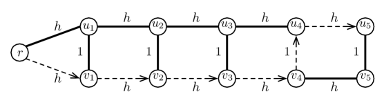
Figure 1: The ladder graph $L_{3}$. Path $P_{4}$ is highlighted with dashed edges.

Consider the paths $P_{1},\ldots,P_{2h-1}$ given by

$$P_{i}=\begin{cases}r,u_{1},u_{2},\ldots,u_{i},v_{i},v_{i+1},v_{i+2},\ldots,v_{2h-1}&\text{if $i$ is odd}\\ r,v_{1},v_{2},\ldots,v_{i},u_{i},u_{i+1},u_{i+2},\ldots,u_{2h-1}&\text{if $i$ is even}\end{cases}$$

Each $P_{i}$ has regret exactly 1 and each node $w\neq r$ lies on precisely $h$ of these paths. So setting $x_{P_{i}}=\frac{1}{h}$ for all $i=1,\ldots,2h-1$, and $x_{P}=0$ for all other paths in $\mathcal{C}_{1}$ yields a solution that covers all the nodes in $V$ to an extent of 1 using $2-\frac{1}{h}$ paths.

The final instance consists of $ch$ copies of $L_{h}$ that share the root $r$ but are otherwise disjoint. We set $k=c(2h-1)$. Taking the above fractional solution for each copy of $L_{h}$, yields a feasible solution to (P3) when $R=1$. Now consider any integer solution with maximum regret less than $2h-1$. Note that any rooted path with regret less than $2h$ can only traverse nodes from a single ladder $L_{h}$. Also, as noted above, if a single path covers all the nodes of some copy of $L_{h}$, then this path has regret at least $2h-1$. Therefore, the solution must use at least $2ch=k+c$ paths. ∎

8 Solving the configuration-style LPs (P) and (P2)

Proof of Lemma 3.1 : We obtain an approximate solution to (P) (reproduced below), by considering the dual problem (D), which has an exponential number of constraints. Recall that $P$ indexes paths in $\mathcal{C}_{R}$.

$$\min \sum_{P}x_{P}$$ (P)

s.t. $$\sum_{P:v\in P}x_{P} \geq 1\qquad \forall v\in V$$ (2)

$$x \geq 0.$$

  $\displaystyle\max$ $\displaystyle\sum_{v}\pi_{v}$ (D) s.t. $\displaystyle\sum_{v\in P}\pi_{v}$ $\displaystyle\leq 1\qquad$ $\displaystyle\forall P$ (3) $\displaystyle\pi$ $\displaystyle\geq 0.$ (4)

The $\pi_{v}$ dual variables correspond to the primal constraints (2). We show that (D) can be solved approximately, and hence (P) can be solved approximately. Separating over the dual constraints (3) amounts to determining, given rewards $\{\pi_{v}\}$ on the nodes, if there is a rooted path of regret at most $R$ that gathers reward more than 1. We try all possible locations $t$ for the end-node of this path; for a given destination $t$, the above problem is an instance of orienteering.

Define $\mathcal{P}(\nu;a):=\{\pi:\eqref{prewd},\ \eqref{noneg},\ \sum_{v}\pi_{v}\geq a\nu\}$. Note that $\mathit{OPT}$ is the largest $\nu$ such that $\mathcal{P}(\nu;1)\neq\emptyset$. We use the $\gamma_{\mathsf{orient}}$-approximation algorithm to give an approximate separation oracle in the following sense. Given $\nu,\pi$, we either show that $\pi/\gamma_{\mathsf{orient}}\in\mathcal{P}(\nu;1)$, or we exhibit a hyperplane separating $\pi$ from $\mathcal{P}(\nu;\gamma_{\mathsf{orient}})$. Thus, for a fixed $\nu$, in polynomial time, the ellipsoid method either certifies that $\mathcal{P}(\nu;\gamma_{\mathsf{orient}})=\emptyset$, or returns a point $\pi$ with $\pi/\gamma_{\mathsf{orient}}\in\mathcal{P}(\nu;1)$. The approximate separation oracle proceeds as follows. We first check if $\sum_{v}\pi_{v}\geq\gamma_{\mathsf{orient}}\nu$, (4) hold, and if not, use the appropriate inequality as the separating hyperplane. Next, for each location $t\in V$, we run the $\gamma_{\mathsf{orient}}$-approximation algorithm for orienteering specified by rewards $\{\pi_{v}\}$, $r$, $t$, and length bound $D_{t}+R$. If in this process we ever obtain a rooted path $P$ with reward greater than 1, then $P\in\mathcal{C}_{R}$ and we return $\sum_{v\in P}\pi_{v}\leq 1$ as the separating hyperplane. Otherwise, for all paths $P\in\mathcal{C}_{R}$, we have $\sum_{v\in P}\pi_{v}\leq\gamma_{\mathsf{orient}}$ and so $\pi/\gamma_{\mathsf{orient}}\in\mathcal{P}(\nu;1)$.

We find the largest value $\nu^{*}$ (via binary search) such that the ellipsoid method run for $\nu^{*}$ (with the above separation oracle) returns a solution $\pi^{*}$ with $\pi^{*}/\gamma_{\mathsf{orient}}\in\mathcal{P}(\nu^{*};1)$; hence, $\nu^{*}\leq\mathit{OPT}$. For any $\epsilon>0$, running the ellipsoid method for $\nu^{*}+\epsilon$ yields a polynomial-size certificate for the emptiness of $\mathcal{P}(\nu^{*}+\epsilon;\gamma_{\mathsf{orient}})$. This consists of the polynomially many violated inequalities returned by the separation oracle during the execution of the ellipsoid method and the inequality $\sum_{v}\pi_{v}\geq\gamma_{\mathsf{orient}}(\nu^{*}+\epsilon)$. By duality (or Farkas’ lemma), this means that here is a polynomial-size solution $x$ to (P) whose value is at most $\gamma_{\mathsf{orient}}(\nu^{*}+\epsilon)$. Taking $\epsilon$ to be $1/\exp(\text{input size})$ (so $\ln\bigl{(}\frac{1}{\epsilon}\bigr{)}$ is polynomially bounded), this also implies that $x$ has value at most $\gamma_{\mathsf{orient}}\nu^{*}\leq\gamma_{\mathsf{orient}}\cdot\mathit{OPT}$.  

Proof of Lemma 6.1 : The proof is similar to the proof of Lemma 3.1, but requires a more refined argument. We again argue that an approximate solution to the dual LP (D2) can be computed efficiently. However, since the dual objective function contains negative terms, even if our approximate separation oracle deems a point $(\pi,z)$ to be feasible, implying that some point in the neighborhood of $(\pi,z)$ is feasible for (D2), we cannot necessarily claim any guarantee on the value of this dual feasible solution relative to the value of $(\pi,z)$ (in fact its value may even be negative!). Consequently, we will need a more refined notion of approximation for the dual LP. This in turn will translate to a approximate solution for the primal, where the approximation is in both the objective value and the satisfaction of the primal constraints.

$$\min \sum_{P\in\mathcal{C}}c^{\mathsf{reg}}(P) x_{P}$$ (P2)

s.t. $$\sum_{P\in\mathcal{C}:v\in P}x_{P} \geq 1\qquad\forall v\in V$$

$$\sum_{P\in\mathcal{C}}x_{P} \leq k$$

$$x \geq 0.$$

  $\displaystyle\max$ $\displaystyle\sum_{v}\pi_{v}$ $\displaystyle-kz$ (D2) s.t. $\displaystyle\sum_{v\in P}\pi_{v}$ $\displaystyle\leq z+c^{\mathsf{reg}}(P)\qquad\forall P\in\mathcal{C}$ (5) $\displaystyle\pi,z$ $\displaystyle\geq 0.$ (6)

Define

$$\mathcal{Q}(\nu;a,b)\ \ :=\ \ \Bigl{\{}(\pi,z):\quad\eqref{newnoneg},\quad\sum_{v\in P}\pi_{v}\leq z+\frac{c^{\mathsf{reg}}(P)}{b}\quad\forall P\in\mathcal{C},\quad\sum_{v}\pi_{v}-a\cdot kz\geq\nu\Bigr{\}}.$$

So $\mathit{OPT}_{R}$ is the largest $\nu$ such that $\mathcal{Q}(\nu;1,1)\neq\emptyset$. For a set $S$ of nodes, let $\pi(S)$ denote $\sum_{v\in S}\pi_{v}$. The separation problem for $\mathcal{Q}(\nu;1,1)$ amounts to finding a rooted path that maximizes $\bigl{(}\pi(P)-c^{\mathsf{reg}}(P)\bigr{)}$. Given a $\gamma_{\mathsf{MEP}}$-approximation algorithm for unweighted MEP, one can obtain a path $P$ such that $\pi(P)-\frac{c^{\mathsf{reg}}(P)}{\beta}\geq\max_{Q\in\mathcal{C}}\bigl{(}\pi(Q)-c^{\mathsf{reg}}(Q)\bigr{)}/\alpha$, where $\alpha=(1-\epsilon)^{-1}$ and $\beta=\gamma_{\mathsf{MEP}}/(1-\epsilon)$. Let $\pi_{\max}=\max_{v}\pi_{v}$. We scale and round the rewards to $\pi^{\prime}_{v}=\left\lfloor\frac{\pi_{v}}{\epsilon\pi_{\max}/n}\right\rfloor$. We try every destination $t$ and run the $\gamma_{\mathsf{MEP}}$-approximation algorithm on the instance with rewards $\{\pi^{\prime}_{v}\}$ (which involves making at most $\frac{n}{\epsilon}$ copies of a node), $r$, $t$. If an optimal solution $P^{*}$ ends at $t$ and achieves reward $\Pi^{*}$ (note that $\Pi^{*}\geq\pi_{\max}$), then we obtain an $r$-$t$ path $P$ with reward at least $\Pi^{*}-\epsilon\pi_{\max}\geq(1-\epsilon)\Pi^{*}$ and $c^{\mathsf{reg}}(P)\leq\gamma_{\mathsf{MEP}}\cdot c^{\mathsf{reg}}(P^{*})$.

We use the above bicriteria approximation algorithm as follows. Given $\nu,\pi,z$, we first check if $\sum_{v}\pi_{v}-\alpha kz\geq\nu$, (6) hold; if not, we use the appropriate inequality as a separating hyperplane between $(\pi,z)$ and $\mathcal{Q}(\nu;\alpha,\beta)$. Next, we use the above algorithm to obtain a rooted path $P$. If $\pi(P)-\frac{c^{\mathsf{reg}}(P)}{\beta}>z$, then we use $\pi(P)\leq z+\frac{c^{\mathsf{reg}}(P)}{\beta}$ as a separating hyperplane between $(\pi,z)$ and $\mathcal{Q}(\nu;\alpha,\beta)$. Otherwise, we know that $\pi(Q)-c^{\mathsf{reg}}(Q)\leq\alpha z$ for all $Q\in\mathcal{C}$, and so $(\pi,\alpha z)\in\mathcal{Q}(\nu;1,1)$.

Thus, for a fixed $\nu$, the ellipsoid method either determines that $\mathcal{Q}(\nu;\alpha,\beta)=\emptyset$ or returns a point $(\pi,\alpha z)\in\mathcal{Q}(\nu;1,1)$. We find the largest value $\nu^{*}$ for which the latter outcome is obtained. So $\nu^{*}\leq\mathit{OPT}_{R}$. For any $\epsilon>0$, running the ellipsoid method with $\nu=\nu^{*}+\epsilon$ returns a polynomial-size certificate for the emptiness of $\mathcal{Q}(\nu;\alpha,\beta)$. Taking $\epsilon=1/\exp(\text{input size})$, this shows that $\nu^{*}$ is an upper bound on the maximum value of $\sum_{v}\pi_{v}-\alpha kz$ subject to (6) and the constraints $\pi(P)-c^{\mathsf{reg}}(P)/\beta\leq z$ for every $P\in\mathcal{C}^{\prime}$, where $\mathcal{C}^{\prime}\subseteq\mathcal{C}$ is the polynomial-size collection of paths corresponding to the path-inequalities returned by the approximate separation oracle. Taking the dual, we obtain the following LP:

$$\min\quad\sum_{P\in\mathcal{C}^{\prime}}\tfrac{c^{\mathsf{reg}}(P)}{\beta}\cdot x_{P}\qquad\text{s.t.}\qquad\sum_{P\in\mathcal{C}^{\prime}:v\in P}x_{P}\geq 1\quad\forall v\in V,\qquad\sum_{P\in\mathcal{C}^{\prime}}x_{P}\leq\alpha k,\qquad x\geq 0.$$

whose optimal value is at most $\nu^{*}$. The optimal solution $x^{*}$ to the above LP satisfies the desired properties.

References

- [1] A. Agrawal, P. Klein, and R. Ravi. When trees collide: An approximation algorithm for the generalized Steiner problem on networks. SIAM Journal on Computing, 24(3):440–456, 1995.
- [2] H. An, R. Kleinberg, and D. Shmoys. Approximation algorithms for the bottleneck asymmetric traveling salesman problem. In Proceedings of APPROX, pages 1–11, 2010.
- [3] A. Asadpour, M. X. Goemans, A. Madry, S. Oveis Gharan, and A. Saberi. An -approximation algorithm for the asymmetric traveling salesman problem. In Proceedings of SODA, 2010.
- [4] N. Bansal, A. Blum, S. Chawla, and A. Meyerson. Approximation algorithms for deadline-TSP and vehicle routing with time windows. In Proceedings of STOC, 2004.
- [5] N. Bansal and M. Sviridenko. The Santa Claus problem. In Proceedings of STOC, pages 31–40, 2006.
- [6] A. Blum, S. Chawla, D. R. Karger, T. Lane, and A. Meyerson. Approximation algorithms for orienteering and discount-reward TSP. SIAM J. Computing, 37(2):653–670, 2007.
- [7] A. Bock, E. Grant, J. Könemann, and L. Sanita. The school bus problem in trees. In Proceedings of ISAAC, 2011.
- [8] A. Bock and L. Sanita. On the approximability of two capacitated vehicle routing problems. In Proceedings of INOC, pages 519–526, 2013.
- [9] D. Chakrabarty and C. Swamy. Facility location with client latencies: linear-programming based techniques for minimum-latency problems. In Proceedings of IPCO, pages 92–103, 2011.
- [10] M. Charikar and B. Raghavachari. The finite capacity dial-a-ride problem. In Proceedings of FOCS, pages 458–467, 1998.
- [11] C. Chekuri, N. Korula, and M. Pál. Improved algorithms for orienteering and related problems. ACM Transactions on Algorithms, 8(3), 2012.
- [12] C. Chekuri, M. Pál. A recursive greedy algorithm for walks in directed graphs. In Proceedings of FOCS, 2005.
- [13] M. Desrochers, J. Desrosiers, and M. Solomon. New optimization algorithm for the vehicle routing problem with time windows. Operations Research, 40:342–354, 1992.
- [14] S. Dobzinski, N. Nisan, and M. Schapira. Approximation algorithms for combinatorial auctions with complement-free bidders. Mathematics of Operations Research, 35(1):1–13, 2010.
- [15] U. Feige. On maximizing welfare when utility functions are subadditive. SIAM Journal on Computing, 39(1):122–142, 2009.
- [16] Z. Friggstad. Multiple traveling salesmen in asymmetric metrics. In Proceedings of APPROX, pages 173–188, 2013.
- [17] Z. Friggstad, M Salavatipour, and Z. Svitkina. Asymmetric traveling salesman path and directed latency problems. In Proceedings of SODA, pages 419–428, 2010.
- [18] M. R. Garey and D. S. Johnson. Computers and Intractability: A Guide to the Theory of NP-Completeness. W. H. Freeman & Co., New York, 1979.
- [19] M. X. Goemans and D. P. Williamson Approximating minimum-cost graph problems with spanning tree edges. Operations Research Letters 16:183–189, 1994.
- [20] M. X. Goemans and D. P. Williamson. A general approximation technique for constrained forest problems. SIAM Journal on Computing, 24:296–317, 1995.
- [21] B. L. Golden, L. Levy, and R. Vohra. The orienteering problem. Naval Research Logistics, 34:307–318, 1987.
- [22] A. Gupta, R. Ravi, and A. Sinha. An edge in time saves nine: LP rounding approximation algorithms for stochastic network design. In Proceedings, 45th IEEE FOCS, pages 218-227, 2004.
- [23] A. Gupta and A. Kumar. A constant-factor approximation for stochastic Steiner forest. In Proceedings, 41st ACM STOC, pages 659–668, 2009.
- [24] M. Haimovich and A. Kan. Bounds and heuristics for capacitated routing problems. Mathematics of Operations Research, 10:527–542, 1985.
- [25] N. Karmarkar and R. Karp. An efficient approximation scheme for the one-dimensional bin-packing problem. In Proceedings of FOCS, pages 312–320, 1982.
- [26] G. Laporte, M. Desrochers, and Y. Nobert. Two exact algorithms for the distance constrained vehicle routing problem. Networks, 14:47–61, 1984.
- [27] J. K. Lenstra, D. B. Shmoys, and É. Tardos. Approximation algorithms for scheduling unrelated parallel machines. Mathematical Programming, 46:259–271, 1990.
- [28] C.-L. Li, D. Simchi-Levi, and M. Desrochers. On the distance constrained vehicle routing problem. Operations research, 40:790–799, 1992.
- [29] V. Nagarajan and R. Ravi. Approximation algorithms for distance constrained vehicle routing problems. Tepper School of Business, Carnegie Mellon University, Pittsburgh, 2008.
- [30] V. Nagarajan and R. Ravi. Approximation algorithms for distance constrained vehicle routing problems. Networks, 59(2):209–214, 2012.
- [31] V. Nagarajan and R. Ravi. The directed orienteering problem. Algorithmica, 60(4):1017–1030, 2011.
- [32] J. Park and B. Kim. The school bus routing problem: A review. European Journal of Operational Research, 202(2):311–319, 2010.
- [33] T. Rothvoss. Approximating bin packing within bins. CS arXiv, January 2013.
- [34] D. B. Shmoys and É. Tardos. An approximation algorithm for the generalized assignment problem. Mathematical Programming, 62:461–474, 1993.
- [35] M. Spada, M. Bierlaire, and T. Liebling. Decision-aiding methodology for the school bus routing and scheduling Problem. Transportation Science, 39(4):477–490, 2005.
- [36] O. Svensson. Santa Claus schedules jobs on unrelated machines. SIAM Journal on Computing, 41(5):1318–1341, 2012.
- [37] P. Toth and D. Vigo, eds. The Vehicle Routing Problem. SIAM Monographs on Discrete Mathematics and Applications, Philadelphia, 2002.