The Pauli principle and magnetism

Abstract

According to Heisenberg, ferromagnetism stems from the Pauli magic mediating between Coulomb interaction and electrons’ spins. The primary aim of this paper is to turn the magic into an algebra by setting a precise bound to the degree a given electron distribution can affect spin. An application of the resulting spin-orbital Pauli constraints to Fe, Co, and Ni provides a new insight into the origin of magnetic moment in these archetypical ferromagnets.

Introduction.

Everyone agrees that the initial form of the Pauli principle – no state can be occupied by more than one electron – is obsolete and must be replaced by the concept of skew-symmetry of a multi-electron wave functions. Nevertheless, in treatment of Fermi-Dirac statistics we tacitely assume that the Pauli condition $\langle\psi|\rho|\psi\rangle\leq 1$ is the only constraint on the fermionic density matrix $\rho$. In fact, there are many more of them, generically given by linear inequalities on eigenvalues of $\rho$ B-D ; Ruskai ; Klyachko08 . For finite dimensional one-electron space $\mathcal{H}$, at least in principle, all Pauli constraints can be found Klyachko08 .

The one electron space $\mathcal{H}=\mathcal{H}_{\ell}\otimes\mathcal{H}_{s}$ splits into orbital and spin degrees of freedom. Here we assume that $N$-electron state $\Psi\in\wedge^{N}\mathcal{H}$ has a well defined total spin $S$ and the respective spin density matrix $\rho_{S}$ along with the orbital one $\rho_{\ell}$. Let $\mu_{1}\geq\mu_{2}\geq\mu_{3}\geq\cdots$ and $\nu_{1}\geq\nu_{2}\geq\nu_{3}\geq\ldots$ be spectra of spin and orbital density matrices normalized to the the unit probability $\sum_{j}\mu_{j}=1$ and to the number of particles $\sum_{i}\nu_{i}=N$ respectively. In this setting the Pauli constraints amount to a system of linear inequalities on orbital and spin occupation numbers $\nu_{i}$, $\mu_{j}$ Klyachko08 . They will be referred below as spin-orbital Pauli constraints. As a toy example, consider the Pauli constraints for $d^{7}$ shell in low spin configuration $S=\frac{1}{2}$ borrowed from Klyachko08

$$\small\begin{array}[]{l}M\leq 3-2(\nu_{3}-\nu_{4});\quad M\geq 2(\nu_{3}-\nu_{5})-3;\\ M\leq 3-2(\nu_{4}-\nu_{5});\quad M\geq 1-2(\nu_{2}-\nu_{4}+2\nu_{5});\\ \hskip 56.9055pt\nu_{3}+\nu_{4}-\nu_{5}\leq 3.\end{array}$$ (1)

Here $M=\mu_{1}-\mu_{2}$ is the maximal possible spin magnetic moment for a given spin density $\mu$ and I skip the initial Pauli constraint $\nu\leq 2$. In a BCC crystal favouring $t_{2g}$ orbitals $\nu_{1}=\nu_{2}=\nu_{3}=a\geq b=\nu_{4}=\nu_{5}$ we get the bound $M\leq 10-5a$ that falls short of the nominal spin-$\frac{1}{2}$ value $M=1\mu_{B}$ for $a>\frac{9}{5}$. It should be emphasized that the spin moment reduction came directly from the Pauli kinematics with no interaction involved.

I will give more realistic examples below and for now put this insight into a historical context. First of all, it sheds light on 80 years old puzzle of reduction atomic spin moments in ferromagnets. The problem was raised by Pauli at Solvay congress on magnetism in 1930 Pauli30 . Being unable to resolve the issue on intra-atomic level he reluctantly conceded that “it seems rather that several atoms should participate” and inscribed the riddle into the list of three open problems in magnetism. Later on Stoner has turned the unsolved Pauli problem into a paradigm of itinerate magnetism

All the earlier atomic theories of ferromagnetism are confronted with the difficulty that the saturation magnetization does not correspond to an integral number of Bohr magnetons per atom, a difficulty which could be met only by an artificial and ad hoc conception of a metal as containing an equilibrium mixture of neutral atoms and ions of different moments, including zero. (Stoner47, , p. 69)

The very existence of the spin-orbital Pauli constraints makes the Stoner’s argument void and relegates it to history books along with its numerous variations repeated in almost every modern text on ferromagnetism

[T]he experimental magnetic moment $\mu=2.2\,\mu_{B}$ is not an integer number, which indicates presence of some fraction of itinerant electrons. Katanin10

The magnetism of the iron-series transition-metal elements is caused by extended delocalized or itinerate electrons. The itinerate character is epitomized by noninteger spin moments per atom […]. (Skomski08, , p. 52)

Today everyone agrees that some degree of itinerancy must be granted to the $d$-electrons in order to explain many basic experimental facts, such as the saturate nonintegral number of Bohr magnetons per atom. Mota86

The idea that the reduction effect comes directly from the Pauli kinematics, as opposed to the ambiguous concept of exchange interaction, goes back to Feynman . He, however, could not fulfill the prophesy since the relevant math was not available at that time.

The current study rests upon a calculation of the Pauli constraints for all high spin $d$-shell configurations. Most of them, whether to good or to bad, turn out to be counterintuitive and defy any simple explanation. Yet that very incomprehensibility makes the Pauli constraints indispensable for an expansion of our insight beyond the horizon of intuition into a new unexplored realm hidden beneath the surface of common sense. I will discuss them at some length in the next section.

The rest of the paper is focused on various manifestations of the Pauli constraints in ferromagnetic iron, cobalt, and nickel. Densities of $d$-electrons in these archetypical ferromagnets were accurately measured by Jauch&Reehuis Jauch07 ; Jauch08 ; Jauch09 . Plugging these data into spin-orbital constraints yields a Pauli upper bound on the spin magnetic moment. For iron it coincides with the actual value $2.22\;\mu_{B}$ of the magnetic moment, see Fig 1. Thus the Pauli constraints provide an accurate account for the observed atomic magnetic moment. A similar saturation of the Pauli bound holds in cobalt, but not in nickel where the spin magnetic moment is far below of that bound.

The last section deals with an impact of the Pauli constraints on quantum statistics. It can be best seen in crossovers between different regimes in magnetisation curve of iron. Indeed, at zero temperature the atomic state in iron saturates three independent Pauli constraints, while at high temperature the Pauli constraints become irrelevant. As the temperature decreases, the spin state saturate the Pauli constraints one by one that effectively quenches certain degrees of freedom and qualitatively changes the thermal evolution. A calculation predicts two such crossovers roughly at about $460^{\circ}$K and $180^{\circ}$K. The first one has been previously reported by Köbler Koebler03 at $467^{\circ}$K, while the second one was buried unnoticed in Pauthenet’s extremely accurate study of high field susceptibility Pauthenet82 , which exhibits a very clean quantum crossover at $200^{\circ}$K shown in Fig 4. See also recent book Koebler09 on the magnetic crossovers phenomenology.

A first glimpse into the Pauli constraints.

Consider a spin polarized system with orbital occupancies $\nu_{1}\geq\nu_{2}\geq\nu_{3}\cdots$. In the simplest case of two spin-polarized electrons the nonzero eigenvalues are evenly degenerated $\nu_{2i-1}=\nu_{2i}$ that gives the simplest constraint beyond the initial Pauli condition $\nu_{i}\leq 1$. In particular, a spin-polarized $d^{2}$-shell must have $\nu=(\nu_{1},\nu_{1},\nu_{3},\nu_{3},0)$. By a similar reason orbital occupancies of spin polarized $d^{3},d^{7},d^{8}$ shells must be of the form $(1,\nu_{2},\nu_{2},\nu_{4},\nu_{4})$, $(\nu_{1},\nu_{1},\nu_{3},\nu_{3},1)$, $(2,\nu_{2},\nu_{2},\nu_{4},\nu_{4})$ respectively Klyachko08 . In particular, sphericall symmetry $\nu=(a,a,a,a,a)$ is incompatible with full spin polarization , i.e. either the charge must be deformed or the atomic spin moment reduced.

When the number of electrons and dimension of the shell increase, the extended Pauli constraints turn into inequalities rather than equations. In that respect they are getting closer to the initial Pauli principle. For three spin-polarized electrons in $f$-shell they are as follows

$$\begin{array}[]{rr}\nu_{2}+\nu_{3}+\nu_{4}+\nu_{5}\leq 2;&\qquad\nu_{1}+\nu_{3}+\nu_{4}+\nu_{6}\leq 2;\cr\nu_{1}+\nu_{2}+\nu_{4}+\nu_{7}\leq 2;&\qquad\nu_{1}+\nu_{2}+\nu_{5}+\nu_{6}\leq 2.\end{array}$$

These constraints hold for any separable spin-orbital state and a failure of any of them is a signature of spin-orbital entanglement. All spinless Pauli constraints for shells of dimension $\leq 10$ can be found in Klyachko08 . Beyond that range only few of them are known, like the following ones for three elelctron shell of even dimension $n$

$$\nu_{i}+\nu_{j}\leq 1,\quad i+j=n+1.$$

They clearly supersede the initial Pauli principle $\nu_{i}\leq 1$.

The purely orbital Pauli constraints allow only to detect an onset of the spin-orbital entanglement and the resulting spin moment reduction with no estimation of its magnitude. To move forward, we have to include into consideration spin density matrix $\rho_{s}$. Joint constraints on both orbital $\nu$ and spin $\mu$ occupancies have been treated theoretically in Klyachko08 . The actual calculation is rather involved. The results are summarised in two tables below.

Spin-orbital Pauli constraints for high spin $d^{7}$ shell
$[0,0,1,-1,-2\mid 0,1,0,2]\leq-1$	$[1,0,0,1,-1\mid-1,0,0,1]\leq 2$
$[0,1,0,-1,-2\mid 0,0,1,2]\leq-1$	$[0,1,1,0,-1\mid-1,0,0,1]\leq 2$
$[0,1,-1,-2,0\mid 0,2,0,1]\leq-1$	$[0,0,1,-1,1\mid 1,-1,0,0]\leq 2$
$[0,1,0,-2,-1\mid 0,1,0,2]\leq-1$	$[0,1,1,-1,0\mid 0,-1,0,1]\leq 2$
$[0,1,-2,-1,0\mid 0,2,1,0]\leq-1$	$[1,-1,0,0,1\mid 1,-1,0,0]\leq 2$
$[1,-2,-1,0,0\mid 1,2,0,0]\leq-1$	$[1,-1,0,0,1\mid 0,1,-1,0]\leq 2$
$[1,-1,0,0,-2\mid 0,1,0,1]\leq-1$	$[1,0,1,-1,0\mid-1,0,0,1]\leq 2$
$[1,0,-1,0,-2\mid 0,0,1,2]\leq-1$	$[0,1,-1,0,1\mid 0,1,-1,0]\leq 2$
$[1,-1,0,-2,0\mid 0,1,2,0]\leq-1$	$[0,0,1,-1,0\mid 1,0,0,0]\leq 1$
$[1,0,0,-2,-1\mid 0,0,1,2]\leq-1$	$[1,-1,0,0,0\mid 1,0,0,0]\leq 1$
$[1,0,-2,-1,0\mid 0,1,2,0]\leq-1$	$[1,0,-1,0,0\mid 0,1,0,0]\leq 1$
$[1,0,-2,-1,0\mid 0,2,0,1]\leq-1$	$[1,0,0,-1,0\mid 0,0,1,0]\leq 1$
$[0,-1,1,-2,0\mid 2,0,0,1]\leq-1$	$[1,0,0,0,-1\mid 0,0,0,1]\leq 1$
$[0,0,1,-2,-1\mid 1,0,0,2]\leq-1$	$[0,1,0,-1,0\mid 0,1,0,0]\leq 1$
$[-1,0,1,-2,0\mid 2,0,1,0]\leq-1$	$[0,0,1,-1,-1\mid 0,0,1,2]\leq 0$
$[1,-2,-1,0,0\mid 2,0,1,0]\leq-1$	$[0,-1,0,-1,1\mid 2,0,0,1]\leq 0$
$[1,-2,0,-1,0\mid 2,0,0,1]\leq-1$	$[0,-1,-1,0,1\mid 1,2,0,0]\leq 0$
$[0,1,1,0,0\mid 0,0,-1,0]\leq 3$	$[-1,0,0,-1,1\mid 2,0,1,0]\leq 0$
$[1,1,0,0,0\mid-1,0,0,0]\leq 3$	$[0,-1,-1,0,1\mid 2,0,1,0]\leq 0$
$[1,0,1,0,0\mid 0,-1,0,0]\leq 3$	$[-1,0,-1,0,1\mid 2,1,0,0]\leq 0$
$[1,0,0,1,0\mid 0,0,-1,0]\leq 3$	$[1,0,1,0,1\mid 1,0,0,0]\leq 5$
$[1,0,0,0,1\mid 0,0,0,-1]\leq 3$	$[1,1,0,0,1\mid 0,1,0,0]\leq 5$
$[-1,0,0,1,2\mid 2,1,-1,0]\leq 4$	$[1,1,1,0,0\mid 0,0,0,1]\leq 5$
$[0,-1,0,1,2\mid 1,2,-1,0]\leq 4$	$[0,0,0,0,1\mid 1,0,0,0]\leq 2$
$[0,1,2,-1,0\mid-1,0,1,2]\leq 4$	$[0,0,1,1,1\mid 1,1,0,0]\leq 5$
$[-1,0,-1,0,1\mid 1,-1,0,0]\leq-1$	$[-1,0,0,1,2\mid 2,0,0,1]\leq 4$
$[-1,-1,0,0,1\mid 1,0,-1,0]\leq-1$	$[-2,-1,0,1,2\mid 2,-1,0,1]\leq 1$
$[1,0,0,0,0\mid 0,0,0,0]\leq 2$	$[0,0,0,0,-1\mid 0,0,0,0]\leq-1$

Spin-orbital Pauli constraints for high spin $d^{8}$ shell
$\quad[0,2,-1,0,1\mid 1,-1,0]\leq 4\quad\,$	$[-1,1,-1,0,0\mid 1,-1,0]\leq-1$
$[0,2,0,1,-1\mid-1,0,1]\leq 4$	$[-1,0,1,-1,0\mid 0,1,-1]\leq-1$
$[0,1,2,-1,0\mid-1,1,0]\leq 4$	$[-1,0,0,1,-1\mid 1,-1,0]\leq-1$
$[0,1,2,0,-1\mid-1,0,1]\leq 4$	$[-1,0,0,1,-1\mid 0,1,-1]\leq-1$
$[0,0,1,2,-1\mid 0,1,-1]\leq 4$	$[0,0,0,-1,-1\mid-1,0,0]\leq-3$
$[0,0,1,2,-1\mid 1,-1,0]\leq 4$	$[0,0,-1,-1,0\mid 0,0,-1]\leq-3$
$[0,1,-1,0,0\mid 1,0,0]\leq 1$	$[0,-1,0,0,-1\mid 0,0,-1]\leq-3$
$[0,1,0,-1,0\mid 0,1,0]\leq 1$	$[0,0,-1,0,-1\mid 0,-1,0]\leq-3$
$[0,1,0,0,-1\mid 0,0,1]\leq 1$	$[0,1,0,1,0\mid 1,0,0]\leq 4$
$[0,0,1,0,-1\mid 0,1,0]\leq 1$	$[0,1,1,0,0\mid 0,1,0]\leq 4$
$[0,0,0,1,-1\mid 1,0,0]\leq 1$	$[0,0,0,1,1\mid 0,0,-1]\leq 3$
$[-1,1,0,0,1\mid 1,-1,0]\leq 2$	$[-1,0,0,0,-1\mid 0,0,0]\leq-3$
$[-1,0,1,1,0\mid 1,-1,0]\leq 2$	$[-1,0,0,0,0\mid 1,0,0]\leq-1$
$[-1,0,1,1,0\mid 0,1,-1]\leq 2$	$[1,0,0,0,0\mid 0,0,0]\leq 2$
$[-1,0,1,0,1\mid 1,0,-1]\leq 2$	$[0,0,0,0,-1\mid 0,0,0]\leq-1$

Here $[a_{1},a_{2},a_{3},a_{4},a_{5}\mid b_{1},b_{2},b_{3}]\leq c$ is a shortcut for spin-orbital constraint

$$a_{1}\nu_{1}+a_{2}\nu_{2}+a_{3}\nu_{3}+a_{4}\nu_{4}+a_{5}\nu_{5}+b_{1}\mu_{1}+b_{2}\mu_{2}+b_{3}\mu_{3}\leq c.$$

In the tables they are grouped into cubicles with the same coefficients $a$, $b$, and $c$ up to an order within $a$ and $b$.

The spin-orbital constraints for high spin configurations $d^{3}$ and $d^{2}$ can be obtained from $d^{7}$ and $d^{8}$ by the particle-hole duality $\nu_{i}\mapsto 2-\nu_{6-i}$ Klyachko08 . The term $d$-shell here refers to an orbital space of dimension 5 with no connotation to a specific physical interpretation.

In the remaining high spin configurations $d^{N}$, $N=1,4,5,6,9$ the Pauli constraints degenerate into equations and can be described as follows.

• For a half-filled shell $N=5$ the multi-electron orbital space $\wedge^{5}\mathcal{H}_{\ell}$ is one dimensional, and the system effectively has only spin degrees of freedom. Formally in this case $\mu_{1}=1,\nu_{1}=5$.

• For $N=4$ spin and orbital occupation numbers are related by the equation $\mu_{i}=1-\nu_{j},i+j=6$. Similar equations $\mu_{i}=\nu_{i}-1$ hold for $N=6$.

• For one electron system $N=1$ the Pauli constraints amount to isospectrality $\mu_{i}=\nu_{i}$, while for one hole ($N=9$) they take the form $\mu_{i}=2-\nu_{j},i+j=6$.

A similar description holds for orbital space $\mathcal{H}_{\ell}$ of any dimension $n$ containing $1,n-1,n,n+1,2n-1$ electrons in a high spin configuration. In particular, there are no nondegenerate spin-orbital constraints in $p$-shells.

Let’s now take a closer look at some $d^{7}$ constraints

$$\nu_{1}+\nu_{i+1}-3 \leq \mu_{i}\leq 1-(\nu_{1}-\nu_{i+1}),\quad i=1\ldots 4,$$

$$M \geq 2(\nu_{2}+2\nu_{3}-\nu_{4})-7.$$ (2)

The lower and the upper bounds on spin occupation numbers $\mu_{i}$ come from the second cubicles in the left and the right columns of the table respectively. Purely orbital constraints $\nu_{1}\leq 2$, $\nu_{5}\geq 1$ in the last line of the table ensure that the upper bound on $\mu_{i}$ is nonnegative.

It is worth to figure out what happens for $\nu_{5}<1$. Clearly, in this case the shell can’t be in a high spin state, but it may be not in a low spin state either if the orbital constraint (1) fails, i.e. $\nu_{3}+\nu_{4}-\nu_{5}>3$. Such a state with indefinite total spin can not come from a spin independent interaction, like the Coulomb one. Thus we arrived at the following claim: For any spin independent interaction in $d^{7}$ shell the following orbital constraint holds

$$\nu_{3}+\nu_{4}-\nu_{5}\leq 3.$$ (3)

For example, no spin independent interaction can produce orbital occupancies like $(1.75,1.75,1.65.1.65,0.2)$.

The lower bound (2) on the maximal magnetic moment $M=3\mu_{1}+\mu_{2}-\mu_{3}-3\mu_{4}$ is just the last constraint in the third cubicle on the left column. None of the constraints gives directly an upper bound on $M$ and one needs a suitable software, like Convex package FranzConv , to extract this information:

$$M\leq 2(\nu_{2}+\nu_{4})-3;\framebox{$M\leq 2(\nu_{1}+\nu_{3}-\nu_{5})-1$}\;\framebox{Fe}$$ (4)

$$M\leq 9-2(2\nu_{1}-\nu_{2}+\nu_{4});\;M\leq 9-2(\nu_{2}+2\nu_{3}-\nu_{4});$$

$$\hskip 28.45274pt\framebox{$M\leq 3\nu_{3}+(\nu_{4}-\nu_{5})-5(\nu_{1}-\nu_{2})$}\;\framebox{Co}$$ (5)

The framed constraints set the actual Pauli bounds on spin magnetic moments for iron and cobalt for experimental orbital occupancies $\nu$. Note also that for spherically symmetric $d^{7}$-shell with equal occupancies $\nu_{i}=\frac{7}{5}$ the first marked inequality gives $M\leq 1.8\,\mu_{B}$. Any excess of this bound must be accompanied by a non-spherical charge deformation, which many researchers considered as a “reminiscence of orbital magnetism” Brewer04 . Pauli constraints provide another interpretation of this effect.

Spin populations in a spherical shell subject to the following Pauli constraints

$$\textstyle\mu_{1}+\mu_{2}\leq\frac{4}{5},\quad\mu_{1}-\mu_{3}\leq\frac{2}{5},\quad\mu_{1}\leq 2\mu_{2}+\mu_{3},$$

that confine the maximal moment $1.8\,\mu_{B}$ to the unique spin configuration $\mu=(\frac{3}{5},\frac{1}{5},\frac{1}{5},0)$.

Surprisingly, the exclusion principle also produces an opposite effect of atomic spin polarization induced by a given charge density. An example of this provides the last inequality in (2) that set a lower bound on the magnetic moment $M$. To estimate the likelyhood of this phenomenon, let’s first calculate constraints on the orbital occupancies compatible with zero spin moment

$$\begin{array}[]{l}\nu_{1}+\nu_{3}-\nu_{4}\leq 2,\quad\nu_{1}+\nu_{4}-\nu_{5}\leq 2,\quad\nu_{2}+\nu_{3}-\nu_{5}\leq 2,\\ \textstyle\nu_{3}-\nu_{4}-\nu_{5}\leq\text{-}\frac{3}{4},\quad\nu_{1}+\nu_{2}\leq\frac{13}{4},\quad\quad\nu_{2}+2\nu_{3}-\nu_{4}\leq\frac{7}{2}.\end{array}$$

Such $\nu$ constitute a tiny fraction $\frac{1085}{31104}\sim 3.5\%$ of the volume of all possible configurations, i.e. a random electron density does produce a nonzero spin moment with probability $0.965$. The ubiquity of this effect raises the question whether $d^{7}$-shell can ever have a free spin for some orbital density $\nu$? As we have seen before, the maximal moment $M=3\,\mu_{B}$ is bounded to the orbital configuraions $\nu=(\nu_{1},\nu_{1},\nu_{3},\nu_{3},1)$, for which the next to the last inequality in the above list leaves the narrow window $\frac{12}{8}\leq\nu_{1}\leq\frac{13}{8}$. A further calculation confirms that the spin population $\mu$ in this interval is indeed free from constraints. An engineering of such a state may be a noble endeavor, but the general notion that atomic spins are free must be abandoned. This never happens in high spin $d^{7}$ configuration neither in BCC nor in FCC cubic field with orbital occupancies $(a,a,a,b,b)$ and $(b,b,a,a,a)$ respectively. However, in low spin $d^{7}$ configuration (1) in FCC crystal field favoring $e_{g}$ orbitals $\nu_{1}=\nu_{2}=a\geq b=\nu_{3}=\nu_{4}=\nu_{5}$ there are no spin-orbital Pauli constraints except the initial one $\nu\leq 2$. It is believed that a transition from low to high spin sector is responsible for the invar effect in FCC Fe-Ni alloys.

In summary, the spin-orbital Pauli constraints contain a wealth of an unexplored physical information. The above examples hardly scratch the surface of it. They provide a quantitative version of the Pauli principle and depend neither on a force or on an interaction involved.

Ferromagnetic iron.

The number of the Pauli constraints is drastically reduced in a cubic solid where the orbital configuration is of the form $\nu=(a,a,a,b,b)$, $a>b$ for a BCC crystal favoring $t_{2g}$ symmetry, and $\nu=(b,b,a,a,a)$, $b>a$ for an FCC structure. For $d^{7}$-shell in a BCC crystal the spin-orbital Pauli constraints amount to 9 inequalities

$$(3-2a)\mu_{1}+(3-2a)\mu_{2}+(2-2a)\mu_{3}+(2-2a)\mu_{4} \leq 0,$$

$$(2a-3)\mu_{1}+(2a-3)\mu_{2}+(2a-4)\mu_{3}+(2a-3)\mu_{4} \leq 0,$$

$$(11-7a)\mu_{1}+(9-7a)\mu_{2}+(7-7a)\mu_{3}+(9-7a)\mu_{4} \leq 0,$$

$$(7a-11)\mu_{1}+(7a-13)\mu_{2}+(7a-11)\mu_{3}+(7a-9)\mu_{4} \leq 0,$$

$$(a-1)\mu_{1}+(a-3)\mu_{2}+(a-2)\mu_{3}+(a-2)\mu_{4} \leq 0,$$

$$(2-a)\mu_{1}-a\mu_{2}+(1-a)\mu_{3}-a\mu_{4} \leq 0,$$

$$(3a-4)\mu_{1}+(3a-6)\mu_{2}+(3a-5)\mu_{3}+(3a-6)\mu_{4} \leq 0,$$

$$(9a-17)\mu_{1}+(9a-15)\mu_{2}+(9a-13)\mu_{3}+(9a-11)\mu_{4} \leq 0,$$

$$(23-15a)\mu_{1}+(17-15a)\mu_{2}+(19-15a)\mu_{3}+(21-15a)\mu_{4} \leq 0,$$

depending on the occupation number $a$ of a $t_{2g}$ orbital.

Below I will focus on the archetypical example of BCC iron whose magnetic moment primary comes from spins of partially filled $3d$-shells. Its electronic density was accurately measured by Jauch&Reehuis Jauch07 . They also addressed the question whether $3d$ electron are indeed localised or itinerate by testing the experimental data versus three available band theory calculations. All of them predict an expansion of the atomic $d$-shell in a solid, while the experiment shows a clear contraction. The authors concluded: no indication for a failure of the localized $3d$ electron model is noticed Jauch07 . The authors also found that the crystal field changes the free atomic configuration $d^{6}$ into $d^{7}$, and $t_{2g}$ electrons make up $62.5(3)\%=5/8$ of the $d$-shell. Whence $a=35/24\approx 1.458(7)$.

Since the spin density matrix commutes with the magnetic symmetry group, the states $|\frac{3}{2}\rangle$, $|\frac{1}{2}\rangle$, $|\text{-}\frac{1}{2}\rangle$, $|\text{-}\frac{3}{2}\rangle$ with definite spin projections onto the magnetization axis are its eigenvectors. The natural spin occupation numbers $\mu=(\mu_{1},\mu_{2},\mu_{3},\mu_{4})$ are just the probabilities to find an iron atom in one of these states.

The Pauli constraints on the magnetic moment $M=3\mu_{1}+\mu_{2}-\mu_{3}-3\mu_{4}$ are shown graphically in Fig. 1. Observe, first of all, that the iron magnetic moment is the maximal possible for the given electron distribution. This suggests that the spins within the Pauli constraints are indeed free. It worth also to note that in the segment $AB$ the saturation magnetic moment and the respective spin distribution are defined by the parameter $a$

$$\textstyle M_{\text{sat}}=7a-8,\quad\mu_{\text{sat}}=\left[\frac{3}{2}(a-1),\frac{1}{2}(a-1),3-2a,0\right].$$

The vertex $A$ corresponds to the spherical atom. The maximal moment in a BCC crystal can not exceed $2.5\,\mu_{B}$ attained at the vertex $B$ with $\mu=\left(\frac{3}{4},\frac{1}{4},0,0\right)$. This is the only point where the atom is always in an up-spin state. In the segment $BC$ the saturation moment and spin occupations are as follows

$$\textstyle M_{\text{sat}}=16-9a,\quad\mu_{\text{sat}}=\left[\frac{1}{2}(9-5a),\frac{1}{2}(a-1),2a-3,0\right].$$

The point $C$ lies on the boundary between high- and low-spin configurations. It is surprising that at the high- to low-spin transition the ordered magnetic moment retains its value $M=1\,\mu_{B}$. Finally, the parameter $a=\frac{14}{9}$ at the point $D$ marks the onset of strictly positive magnetic moment.

Figure 1: The Pauli constraints on spin magnetic moment for $d^{7}$ configuration in BCC symmetry versus the occupation number $a$ of a $t_{2g}$ orbital. All points within the pentagon $ABCDE$ are admissible. The black dot represents iron’s data.

Cobalt and nickel spin moments.

Below we calculate Pauli bounds on spin moment for cobalt and nickel and compare them with the following experimental data deduced from gyromagnetic ratios Stearns84 and the total moments Pauthenet82

$$M^{\text{Fe}}_{\text{tot}} =2.226\,\mu_{B}; M^{\text{Fe}}_{\text{spin}} =2.143\,\mu_{B}; M^{\text{Fe}}_{\text{orb}} =0.083\,\mu_{B};$$

$$M^{\text{Co}}_{\text{tot}} =1.729\,\mu_{B}; M^{\text{Co}}_{\text{spin}} =1.577\,\mu_{B}; M^{\text{Co}}_{\text{orb}} =0.152\,\mu_{B};$$

$$M^{\text{Ni}}_{\text{tot}} =0.619\,\mu_{B}; M^{\text{Ni}}_{\text{spin}} =0.563\,\mu_{B}; M^{\text{Ni}}_{\text{orb}} =0.056\,\mu_{B}.$$

At low temperature cobalt has hexagonal crystal structure that splits $d^{7}$-shell into three sectors

$$a_{g}=\langle 3z^{2}-r^{2}\rangle,\quad e_{g}=\langle xz,yz\rangle,\quad e_{g}^{\prime}=\langle xy,x^{2}-y^{2}\rangle$$

spanned by eigenvectors of the orbital moment operator $L_{z}=i(x\partial_{y}-y\partial_{x})$: $a_{g}=|0\rangle$, $e_{g}=|\pm 1\rangle$, $e_{g}^{\prime}=|\pm 2\rangle$. Here are their experimental orbital populations $(a,b,b,c,c)=(\nu_{1},\nu_{2},\nu_{3},\nu_{4},\nu_{5})$ found by Jauch&Reehuis Jauch09

$$a=1.846(22);\quad b=1.2935(80);\quad c=1.2835(95).$$

They set the Pauli bound (5) on spin magnetic moment

$$M^{\mathrm{Co}}_{\text{spin}} \leq 3\nu_{3}+(\nu_{4}-\nu_{5})-5(\nu_{1}-\nu_{2})$$ (6)

$$=8b-5a=1.118\,\mu_{B},$$

which is clearly incompatible with the experimental value $M^{\mathrm{Co}}_{\text{spin}}=1.577\,\mu_{B}$. The discrepancy came from the fact that Jauch&Reehuis measured populations of the subshells, while the Pauli constraints refer to eigenvalues of the density matrix. In absence of the orbital moment they would be the same, but otherwise we have to take it into account by a variation of the orbital eigenstates’ occupancies $(a,b,b,c,c)\mapsto(a,b+\varepsilon,b-\varepsilon,c+\delta,c-\delta)$ that preserves the number of electrons in the subshells $|0\rangle$, $|\pm 1\rangle$, $|\pm 2\rangle$ and matches the experimental value of the orbital moment $M_{\text{orb}}^{\text{Co}}=2\varepsilon+4\delta=0.152\mu_{B}$.

The Pauli bound (6) depends on the exact order of the occupancies $a,b\pm\varepsilon,c\pm\delta$. Observe that within the error bar $b=c$ and therefore the order is determined by the type of inequality $\varepsilon\lessgtr\delta$. For $\varepsilon<\delta$ we have

$$(\nu_{1},\nu_{2},\nu_{3},\nu_{4},\nu_{5})=(a,c+\delta,b+\varepsilon,b-\varepsilon,c-\delta)$$

that still gives too low Pauli bound

$$M_{\text{spin}}^{\text{Co}} \leq 3\nu_{3}+(\nu_{4}-\nu_{5})-5(\nu_{1}-\nu_{2})$$

$$=3(b+\varepsilon)+(b-\varepsilon)-(c-\delta)-5(a-c-\delta)$$

$$=7(2-a)+2\varepsilon+6\delta=1.078+M_{\text{orb}}+2\delta$$

$$\textstyle\leq 1.078+\frac{3}{2}M_{\text{orb}}=1.306\,\mu_{B}.$$

For $\varepsilon>\delta$ we have to switch $b\leftrightarrows c$ and $\varepsilon\leftrightarrows\delta$ that gives

$$M_{\text{spin}}^{\text{Co}}\leq 7(2-a)+6\varepsilon+2\delta.$$

When $\delta=0$, i.e. the orbital moment comes entirely from $e_{g}$ subshell, we get the maxmal Pauli bound

$$M_{\text{spin}}^{\text{Co}}\leq 7(2-a)+6\varepsilon=7(2-a)+3M^{\text{Co}}_{\text{orb}}=1.534\mu_{B},$$

which is slightly less than the experimental value $1.577\,\mu_{B}$ but indistinguishable from it in view of the orbital occupancy uncertainty $a=1.846(22)$.

In summary, there is unique way to reconcile the orbital moment of cobalt with Pauli constraints. The moment comes from $e_{g}$ subshell and has minimal possible value compatible with the Pauli bound. The latter, in turn, coincides with the observed spin moment. In a sense, the ferromagnetic order parameter generates the orbital moment to raise the Pauli bound by about 40%. That kind of behavior can be expected in the elemental ferromagnet with strongest known magnetic interaction as seen in its high Curie temperature.

For nickel, which is the weakest elemental ferromagnet, the above analysis based on the Pauli constraints is inconclusive. There are four Pauli bounds on spin magnetic moment $M=2\mu_{1}-2\mu_{3}$ for high spin $d^{8}$ configuration

$$M \leq\nu_{1}-\nu_{2}+\nu_{3}-\nu_{4}+\nu_{5}, M \leq 2\nu_{1}-2\nu_{3}-2\nu_{5}+4,$$

$$M \leq 2\nu_{2}-2\nu_{4}+4\nu_{5}-4, M \leq 4\nu_{3}+2\nu_{4}-2\nu_{2}-4,$$

where the orbital occupancies are subject to additional constraints $\nu_{1}\leq 2$, $\nu_{1}+\nu_{5}\geq 3$. When the latter one fails the shell collapses into a nonmagnetic spin $S=0$ state. Such collapse can’t happen in FCC crystal with orbital occupancies $(a,a,b,b,b)$ favoring $e_{g}$ orbitals but may occur in BCC or tetragonal environment. Apparently this happens in Ni alloy with about 12 atomic percents of vanadium, so that in average a Ni atom has about 1.5 impurities among its 12 nearest neighbors that may reverse the inequality $\nu_{1}+\nu_{5}\geq 3$.

For spherically symmetric shell with equal occupancies $\nu_{i}=\frac{8}{5}$ the second bound gives $M\leq\frac{4}{5}=0.8\mu_{B}$. None of the first three constraints can produce a smaller bound for no orbital occupancies. Therefore nickel spin moment $M_{\text{spin}}^{\text{Ni}}=0.563\mu_{B}$ can saturate, if any, only the last constraint. However, the orbital occupancies $\nu=(a,a,b,b,b)$ of $e_{g}$ and $t_{2g}$ subshells found in Jauch08

$$\textstyle n_{e}=2a=3.475(16),\qquad n_{t}=3b=4.525(16),$$

give the lowest Pauli bound $M\leq 1.442\mu_{B}$, coming from the first constraint, which is not even close to the actual value. For cobalt we have found unique way to comply with the Pauli constraints, while for nickel they hold from the beginning and any change without additional experimental data would be purely speculative. There is no reason to believe that for a weak ferromagnetic interaction the Pauli spin bound must be saturated.

Pauli constraints and statistics.

The next example deals with an impact of the Pauli constraints on spin statistics. To begin with, consider a system of noninteracting free spins in a lattice at temperature $T$ and magnetic field $H$. Its thermal properties are governed by Helmholtz free energy per site

$$F(\mu)=-Hm\cdot\mu-k_{B}TS(\mu),$$ (7)

where $m$ and $\mu$ are vectors of possible local quantized magnetic moments $m_{i}$ and the respective probabilities $\mu_{i}$, $S(\mu)=-\sum\mu_{i}\log\mu_{i}$ is the magnetic entropy. The thermal equilibrium corresponds to the minimum of $F(\mu)$ given by the Gibbs canonical distribution

$$\textstyle\mu_{i}\sim e^{m_{i}\beta},\quad\beta=H/k_{B}T.$$ (8)

In real solids the orbital density matrix of an atom is fixed by the Coulomb crystal field. This in turn imposes Pauli constraints on the probabilities $\mu_{i}$ to find an atom in a given spin state. As a result, the thermal equilibrium is attained at a relative minimum of the free energy taken over the admissible probabilities $\mu$ that form the so called moment polytope. Its boundary separates available spin configurations from forbidden ones and plays a role similar to the Fermi surface. Fig. 2 shows it for BCC iron.

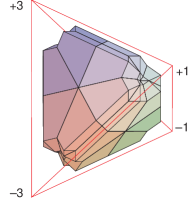
Figure 2: The moment polytope for iron inside the tetrahedron with barycentric coordinates $\mu$. The numbers indicate magnetic moments at vertices of the tetrahedron.

The actual thermal evolution in BCC configuration $d^{7}$ is rather complicated and strongly depends on the orbital occupation number $a$. The experimental value $a=\frac{35}{24}$ for iron falls into the interval $\left[\frac{7}{5},\frac{19}{13}\right]$ where the evolution can be described as follows.

It begins with the uniform distribution at $\beta=0$ and follows Gibbs law (8) until $\mu$ saturates the third Pauli constraint in the list of 9 constraints on page Ferromagnetic iron., turning it into equation which we write in the symbolic form

$$c_{1}\mu_{1}+c_{2}\mu_{2}+c_{3}\mu_{3}+c_{4}\mu_{4}=0.$$ (9)

This happens at the critical value

$$\textstyle\beta_{1}=\frac{1}{2}\log\alpha,\quad c_{1}\alpha^{3}+c_{2}\alpha^{2}+c_{3}\alpha+c_{4}=0,\quad\alpha>1.$$ (10)

Starting from this point the equilibrium state evolves along the saturated facet (9) with the Gibbs distribution replaced by

$$\textstyle\mu_{i}\sim e^{m_{i}\beta+\gamma c_{i}},$$ (11)

where the Lagrange multiplier $\gamma$ is determined by equation of the facet (9)

$$\textstyle\sum_{i}c_{i}e^{m_{i}\beta+\gamma c_{i}}=0.$$

This form persists until the second critical point

$$\textstyle\beta_{2}=\frac{1}{4}\log\frac{20-12a}{19-13a}$$ (12)

where the thermal trajectory hits the first Pauli constraint in the same list turning it into equation

$$d_{1}\mu_{1}+d_{2}\mu_{2}+d_{3}\mu_{3}+d_{4}\mu_{4}=0.$$ (13)

From this point on the thermal equilibrium

$$\mu_{i}\sim e^{m_{i}\beta+\gamma c_{i}+\delta d_{i}}$$ (14)

evolves along the intersection of two facets (9) and (13). The parameters $\gamma,\delta$ are fixed by the facets’ equations

$$\textstyle\sum_{i}c_{i}e^{m_{i}\beta+\gamma c_{i}+\delta d_{i}}=0,\qquad\sum_{i}d_{i}e^{m_{i}\beta+\gamma c_{i}+\delta d_{i}}=0.$$

As $\beta\rightarrow\infty$ the equilibrium eventually freezes up at the vertex of the moment polytope

$$\textstyle\mu_{\text{sat}}=\left[\frac{3}{2}(a-1),\frac{1}{2}(a-1),3-2a,0\right]$$ (15)

with the maximal magnetic moment $M_{\text{sat}}=7a-8$.

In real ferromagnets, the internal field $H$ entering in the parameter $\beta=H/k_{B}T$ is an unknown function of the local magnetic moment $M=3\mu_{1}+\mu_{2}-\mu_{3}-3\mu_{4}$. In a way of illustration assume, following Weiss, that $H$ is proportional to $M$. Figure 3 shows the resulting magnetization curve.

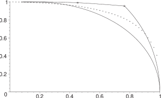
Figure 3: Reduced magnetization $M/M_{\text{sat}}$ versus reduced temperature $T/T_{C}$ for Weiss spin-3/2 model, its modification by the Pauli constraints discussed in the text, and the experimental points for iron Crangle71 . Circles mark the critical points.

Clearly, the spin-orbital Pauli constraints change the temperature behavior both quantitatively and qualitatively. The latter modification, epitomized in the critical points, could be seen in the actual thermal evolution as crossovers between the different physical regimes (8), (11), (14).

The experimental value $a=\frac{35}{24}$ gives critical parameters $\beta_{1}=0.55429$, $\beta_{2}=1.02359$ and the respective magnetic moments $M_{1}/M_{\text{sat}}=0.95585$, $M_{2}/M_{\text{sat}}=0.99296$. By interpolation of the magnetization data Crangle71 the latter can be converted into critical temperatures $T_{1}=461^{\circ}\,\text{K}$ and $T_{2}=176^{\circ}\,\text{K}$ where the crossovers are expected to happen. Above $T_{1}$ spins detach from a direct influence of the lattice and follows usual Weiss theory with no additional Pauli constrains. Therefore it may be not surprising that $T_{1}$ essentially coincides with Debye temperature of iron. The numerical value of $T_{2}$ is very sensitive to small variations of $a$ and should be considered as a rough estimation.

The first critical point can be identified with a crossover at $467^{\circ}\,\text{K}$ previously reported by Köbler Koebler03 , At the second one, the angle between two adjacent segments of the modified Weiss curve in Fig. 3 is too small to see the crossover directly in the magnetization $M(T)$. Therefore we look for the effect in its derivative $\chi_{{}_{HF}}(T)=\frac{\partial M(T)}{\partial H_{\text{ext}}}$ measured at an external field $H_{\text{ext}}$ high enough to make iron crystal a single magnetic domain. The experimental data Pauthenet82 are shown in Fig. 4 together with a quadratic component that may come from the Bloch correction to Pauli paramagnetism Bloch29 or any other source unaffected by the Pauli constraints. The residue shows a sharp crossover around $200^{\circ}\,\text{K}$.

Decreasing the reported orbital occupation number $a=\frac{35}{24}$ by negligible quantity 0.00085, well within the error bar $\pm 0.007$, gives the critical temperatures $T_{1}=465^{\circ}\,\text{K}$, $T_{2}=200^{\circ}\,\text{K}$ compatible with both observations.

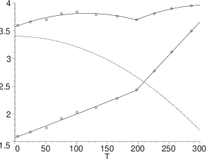
Figure 4: High field susceptibility $\chi_{{}_{HF}}$ for iron Pauthenet82 in units $10^{-6}\text{cm}^{3}/g$ versus temperature in $K^{\circ}$ (the upper curve), its quadratic component $aT^{2}+b$ (shown in dots), and the residue representing the pure quantum crossover effect.

Crossover phenomena are widely spread in magnetic compounds. They have been collected and classified in recent book Koebler09 which may well contain more examples of physical effects caused by the spin-orbital Pauli constraints. Among possible reasons for the crossover phenomena the authors mentioned a change in the number of relevant spin states. This sounds as a paraphrase of the description given above: crossing a critical point turns a Pauli inequality into the equation that effectively reduces available spin degrees of freedom.

Conclusion.

This study rests upon a novel concept of spin-orbital Pauli constraints that provide a quantitative version of the Pauli principle. Being universal and ubiquitous they may have many applications ranging from chemistry to nuclear physics. This paper, however, is focused on ferromagnetism as the most striking and straightforward macroscopic manifestation of spin.

Unfortunately till now there is no rigorous theory of ferromagnetism, mainly because in non-relativistic quantum mechanics spins are not directly involved in the interaction and respond only to a still not fully understood force-free Pauli magic. The latter challenges monopoly of Newton’s culture of force Wilczek04 , but due to its intractability is often substituted by a spin dependent exchange interaction. For those who take it soundly I recall the celebrated Lieb-Mattis theorem LiebMattis ; Peierls79 : For a system of electrons confined to a line and subject to an arbitrary symmetric spin independent interaction the ground state can’t be magnetic. At the same time the exchange approximation applied to a suitable system of that type gives rise to the Heisenberg model with a magnetic ground state. A ghost of this artefact will follow us forever and may show up any time the exchange interaction is invoked.

It should be also emphasized that spin independent hamiltonian commutes with the total spin $S$ and makes it a well defined quantum number. Therefore a precursor of ferromagnetism must be a high total spin sector, from which a ferromagnetic state may emerge by breaking its spin degeneracy. Any surrogate spin dependent Hamiltonian would kill this fundamental truth. This scenario essentially calls for a version of Hund’s rule that determines the total spin state of a multi-electron system. As we have seen above admissible electron densities depend on the total spin. For example, $d^{7}$ shell must be in a low spin state if $\nu_{5}<1$ and $d^{8}$ shell collapses into a spinless state for $\nu_{1}+\nu_{5}<3$.

Anyway, the spin-orbital Pauli constraints provide a unique known mechanism that affects noninteracting spins. Therefore they must play a crucial role in formation of a ferromagnetic state. In many cases the natural orbital occupancies $\nu_{i}$ determine the total spin sector.

To support this claim, the Pauli constraints were calculated for all high spin $d$-shell configurations and tested in ferromagnetic iron, and to a smaller extend in cobalt and nickel. It turns out that for iron and cobalt, where the ferromagnetic interaction is strong and epitomised in high Curie temperature, the spin magnetic moments attain maximal values allowed by the Pauli constraints. This may be the first experimental support of relevance the Pauli constraints. This result also resolves 80 years old Pauli problem on the origin of reduction the atomic magnetic moments in ferromagnets. For nickel where the ferromagnetic interaction is much smaller the actual moment is below the Pauli bound.

We are gratefully acknowledge W. Pauli for a valuable insight.

References

- (1) R. E. Borland and K. Dennis, J. Phys. B 5, 7 (1972);
- (2) M. B. Ruskai, J. Phys. A 4, F961 (2007).
- (3) M. Altunbulak and A. Klyachko, The Pauli principle revisited, Commun. Math. Phys. 292, 287–322 (2008).
- (4) E.C. Stoner, Ferromagnetism, Rep. Prog. Phys. 11 43 (1947).
- (5) A.A. Katanin et al, Phys. Rev. B 81, 045117 (2010).
- (6) R. Skomski, Simple models of magnetism. Oxford Univ. Press, 2008.
- (7) R. Mota and M. D. Coutinho-Filho, Phys. Rev. B 33, 7724 (1986).
- (8) W. Jauch and M. Reehuis, Electron density distribution in -iron: A -ray diffraction study. Phys. Rev. B 76, 235121 (2007).
- (9) W. Jauch and M. Reehuis, Electron density distribution in ferromagnetic nickel: A -ray diffraction study, Phys. Rev. B 78, 235113 (2008).
- (10) W. Jauch and M. Reehuis, Electron density distribution in hexagonal cobalt: A -ray diffraction study, Phys. Rev. B 80, 125126 (2009).
- (11) W. Pauli in Le magnétisme, Rapports et discussions du Sixieme Conseil de Physique, tenu a Bruxelles du 20 au 25 Octobre 1930, sous les auspices de l’Institut International de Physique Solvay (Gauthier-Villars, Paris, 1932).
- (12) L. Hoddeson, G. Baym, and M. Eckert, Rev. Mod. Phys. 59, 287 (1987).
- (13) J. Crangle and G.M. Goodman, Proc. Roy. Soc. Lond. A 321, 477 (1971).
- (14) U. Köbler, J. Englich, O. Hupe, J. Hesse, Effective spin quantum numbers in iron, cobalt and nickel, Physica B 339, 156–163 (2003).
- (15) M.B. Stearns, in Magnetic Properties of 3d, 4d, and 5d Elements, Alloys and Compounds, edited by K.-H. Hellewege and O. Madelung, Landolt-Börnstein, New Series Vol. III. (Springer, Berlin, 1987).
- (16) R. Pauthenet, J. Appl. Phys. 53, 8187 (1982).
-
(17)
M. Franz, Convex, a Maple package for convex geometry,
http:\\www-fourier.ujf-grenoble.fr\~franz\convex - (18) F. Bloch, Z. Physik 53, 216 (1929).
- (19) U. Köbler & A. Hoser, Renormalization group theory: Impact on experimental magnetism (Springer, Heidelberg, 2009).
- (20) W.D. Brewer, A. Scherz, C. Sorg, H. Wende, K. Baberschke, P. Bencok, and S. Frota-Pesso, Direct observation of orbital magnetism in cubic solids. Phys. Rev. Lett., 93 077205 (2004).
- (21) F. Wilczek, Physics Today 10, 11 (2004); 11, 10 (2004); 7, 10 (2005).
- (22) E. Lieb and D. Mattis, Theory of ferromagnetism and the ordering of electronic energy levels. Phys. Rev. 125 164 (1962).
- (23) R. Peierls, Surprises in theoretical physics. Princeton University Press, Princeton, 1979.
- (24) A. Tanaka, and H. Tasaki, Metallic Ferromagnetism in the Hubbard Model: A Rigorous Example. Phys. Rev. Lett., 98 116402 (2007).
- (25) I. Yang, S.Y. Savrasov, and G. Kotliar, Phys. Rev. Lett. 87, 216405 (2001).