Paras Naik
on behalf of the LHCb Collaboration

School of Physics
University of Bristol, Bristol, United Kingdom

Amplitude analysis is a powerful tool to study the properties of intermediate resonances produced in the decays of $B$ mesons. At LHCb we have studied $B^{\pm}\to X(3872)K^{\pm}$, where $X(3872)\to J/\psi\pi^{+}\pi^{-}$, to determine the quantum numbers of the $X(3872)$, and $B^{\pm}\to p\overline{p}K^{\pm}$ to learn more about $(c\overline{c})\to p\overline{p}$ transitions. We also exploit the spin of the $J/\psi$ to perform amplitude analyses of the decays $\kern 1.79993pt\overline{\kern-1.79993ptB}{}^{0}_{(s)}\to J/\psi\pi^{+}\pi^{-}$ and $\kern 1.79993pt\overline{\kern-1.79993ptB}{}^{0}_{(s)}\to J/\psi K^{+}K^{-}$. Our results use 1.0 fb^-1 of data taken in 2011 from $\sqrt{s}=7$ TeV $pp$ collisions, provided by the LHC.

PRESENTED AT

The 6^th International Workshop on Charm Physics
(CHARM 2013)
Manchester, UK, 31 August – 4 September, 2013

1 Introduction

The dominant weak decay $b\to c$ results in the production of charmed states in $B$ meson decays that can be well-explored by the LHCb experiment. The following is a summary of how exploiting charmed states in $B$ decays at LHCb has lead to a better understanding of both. Our results use 1.0 fb^-1 of data from $\sqrt{s}=7$ TeV $pp$ collisions, provided by the LHC in 2011. This data was collected by the LHCb detector (described in Refs. [1, 2]).

2 Measurement of the $X(3872)$ quantum numbers via $B^{\pm}\to X(3872)K^{\pm}$ decays [3]

The $X(3872)$ was discovered in $B^{+}$ decays by the Belle experiment in 2003 [4], and has been confirmed by several other experiments [5, 6, 7]. $X(3872)$ production has most recently been studied at the LHC [8, 9], however the nature of the $X(3872)$ remains unclear. The open explanations for this state are conventional charmonium and exotic states such as $D^{*0}\overline{D}{}^{0}$ molecules [10], tetra-quarks [11], or their mixtures [12]. To determine the best explanation, we need to determine the quantum numbers $J$ (total angular momentum), $P$ (parity), and $C$ (charge-conjugation) of the $X(3872)$. The CDF experiment analyzed three-dimensional (3D) angular correlations in a sample of inclusively-reconstructed $X(3872)\to J/\psi\pi^{+}\pi^{-}$ , $J/\psi\to\mu^{+}\mu^{-}$ decays [13]. A $\chi^{2}$ fit of $J^{PC}$ hypotheses to the binned 3D distribution of the $J/\psi$ and $\pi\pi$ helicity angles ($\theta_{J/\psi}$, $\theta_{\pi\pi}$) [14, 15, 16], and the angle between their decay planes, excluded all spin-parity assignments except for $1^{++}$ or $2^{-+}$. The Belle collaboration concluded that their data were equally well described by the $1^{++}$ and $2^{-+}$ hypotheses, by studying one-dimensional distributions in three different angles [17]. The BaBar experiment used information from $X(3872)\to\omega J/\psi$, $\omega\to\pi^{+}\pi^{-}\pi^{0}$ events to favor the $2^{-+}$ hypothesis, which had a confidence level (CL) of $68\%$, over the $1^{++}$ hypothesis, but the latter was not ruled out (CL $=7\%$) [18]. The angular correlations in the $B^{+}$ decay carry significant information about the $X(3872)$ quantum numbers. A first analysis of the complete five-dimensional angular correlations of the $B^{+}\to X(3872)K^{+}$, $X(3872)\to J/\psi\pi^{+}\pi^{-}$, $J/\psi\to\mu^{+}\mu^{-}$ decay chain has been performed using the 2011 LHCb data sample. A fit to the data yields $313\pm 26$ $B^{\pm}\to X(3872)K^{\pm}$ candidates. To discriminate between the $1^{++}$ and $2^{-+}$ assignments we use the likelihood-ratio test, which in general provides the most powerful test between two hypotheses [19]. The probability distribution function (PDF) for each $J^{PC}$ hypothesis, $J_{X}$, is defined in the 5D angular space $\Omega\equiv$ $(\cos\theta_{X},\cos\theta_{\pi\pi},\Delta\phi_{X,\pi\pi},\cos\theta_{J/\psi},\Delta\phi_{X,J/\psi})$ by the normalized product of the expected decay matrix element (${\cal M}$) squared and of the reconstruction efficiency ($\epsilon$), ${\rm PDF}(\Omega|J_{X})=|{\cal M}(\Omega|J_{X})|^{2}\,\epsilon(\Omega)/I(J_{X})$, where $I(J_{X})=\int|{\cal M}(\Omega|J_{X})|^{2}\,\epsilon(\Omega){\it d}\Omega$. $\theta_{X}$ is the $X(3872)$ helicity angle, and $\Delta\phi_{X,\pi\pi}=\phi_{X}-\phi_{\pi\pi}$ and $\Delta\phi_{X,J/\psi}=\phi_{X}-\phi_{J/\psi}$ are the angles between the $X(3872)$ decay plane and $\pi\pi$ or $J/\psi$ decay planes, respectively. We follow the approach adopted in Ref. [13] to predict the matrix elements.

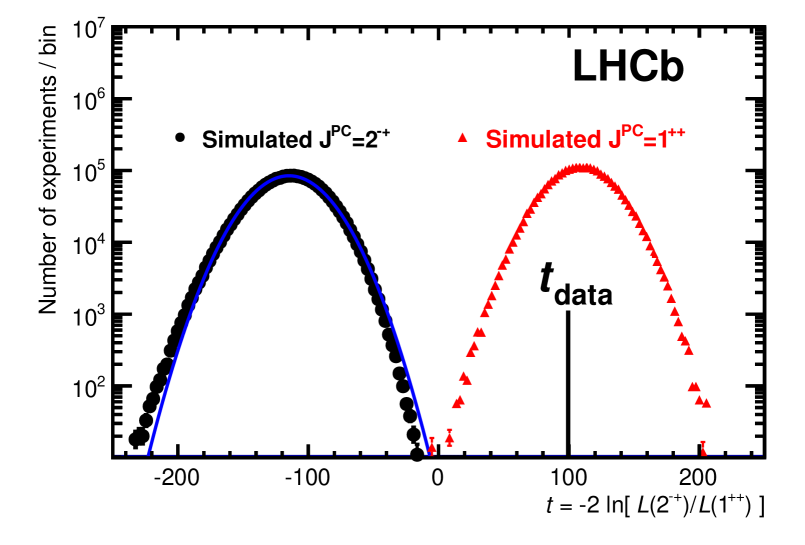
Figure 1: Distribution of the test statistic $t$ for the simulated experiments with $J^{PC}=2^{-+}$ (black circles on the left) and with $J^{PC}=1^{++}$ (red triangles on the right). A Gaussian fit to the $2^{-+}$ distribution is overlaid (blue solid line). The value of the test statistic for the data, $t_{\rm data}$, is shown by the solid vertical line.

We define a test statistic $t=-2\ln[{\cal L}(2^{-+})/{\cal L}(1^{++})]$. The background in the data is subtracted in the log-likelihoods using the sPlot technique [20]. Positive (negative) values of the test statistic for the data, $t_{\rm data}$, favor the $1^{++}$ ($2^{-+}$) hypothesis. The value of the test statistic observed in the data is $t_{\rm data}=+99$, favoring the $1^{++}$ hypothesis. The value of $t_{\rm data}$ is compared with the distribution of $t$ in the simulated experiments to determine a $p$-value for the $2^{-+}$ hypothesis via the fraction of simulated experiments yielding a value of $t>t_{\rm data}$. As shown in Fig. 1, the distribution of $t$ is reasonably well approximated by a Gaussian function. Based on the mean and root mean square spread of the $t$ distribution for the $2^{-+}$ experiments, this hypothesis is rejected with a significance of $8.4\sigma$. Integrating the $1^{++}$ distribution from $-\infty$ to $t_{\rm data}$ gives ${\rm CL}~{}(1^{++})=34\%$. This unambiguously establishes that $J^{PC}$ for the $X(3872)$ state is $1^{++}$.

3 Study of the $p\overline{p}$ charmonium resonances in
$B^{\pm}\to p\overline{p}K^{\pm}$ decays [21]

The $B^{+}\to p\overline{p}K^{+}$ decay offers a clean environment to study $c\overline{c}$ states and charmonium-like mesons that decay to $p\overline{p}$, and to search for glueballs or exotic states. Measurements of intermediate charmonium-like states, such as the $X(3872)$, are important to clarify their nature [3, 22] and to determine their partial width to $p\overline{p}$, which is crucial to predict the production rate of these states in dedicated experiments [23]. BaBar and Belle have previously measured the $B^{\pm}\to p\overline{p}K^{\pm}$ branching fraction, including contributions from the $J/\psi$ and $\eta_{c}(1S)$ intermediate states [24, 25]. The LHCb data sample allows the study of substructures in the $B^{+}\to p\overline{p}K^{+}$ decays with a sample ten times larger than those available at previous experiments. The signal yields for the charmonium contributions, $B^{+}\to(c\overline{c})K^{+}\to p\overline{p}K^{+}$, are determined by fitting the $p\overline{p}$ invariant mass distribution of $B^{+}\to p\overline{p}K^{+}$ candidates within the $B^{+}$ mass signal window, $|M_{p\overline{p}K^{+}}-M_{B^{+}}|<50{\rm MeV/}c^{2}$. An unbinned extended maximum likelihood fit to the $p\overline{p}$ invariant mass distribution, shown in Fig. 2, is performed over the mass range $2400-4500~{}{\rm MeV/}c^{2}$.

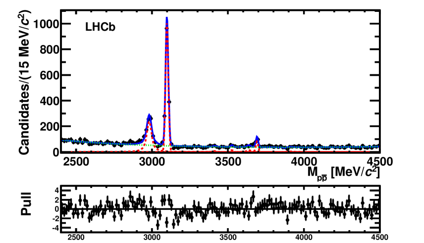
Figure 2: Invariant mass distribution of the $p\overline{p}$ system for $B^{+}\to p\overline{p}K^{+}$ candidates within the $B^{+}$ mass signal window, $|M(p\overline{p}K^{+})-M_{B^{+}}|<50{\rm MeV/}c^{2}$. The dotted lines represent the Gaussian and Voigtian functions (red) and the dashed line the smooth function (green) used to parametrize the signal and the background, respectively. The bottom plot shows the pulls.

We define the ratio of branching fractions for each resonant “mode” as follows:

$${\cal R}({\rm mode})=\frac{{\cal B}(B^{+}\to{\rm mode}~{}K^{+}\to p\overline{p}K^{+})}{{\cal B}(B^{+}\to J/\psi~{}K^{+}\to p\overline{p}K^{+})},$$ (1)

where “mode” corresponds to the intermediate $\eta_{c}(1S)$, $\psi(2S)$, $\eta_{c}(2S)$, $\chi_{c0}(1P)$, $h_{c}(1P)$, $X(3872)$, or $X(3915)$ states. Final results for all intermediate modes are given in Ref. [21]. The total branching fraction, its charmless component $(M_{p\overline{p}}<2.85{\rm GeV/}c^{2})$ and the branching fractions via the resonant $c\overline{c}$ states $\eta_{c}(1S)$ and $\psi(2S)$ relative to the decay via a $J/\psi$ intermediate state are:

$$\frac{{\mathcal{B}}(B^{\pm}\to p\overline{p}K^{\pm})_{\rm total}}{{\mathcal{B}}(B^{+}\to J/\psi K^{+}\to p\overline{p}K^{+})}= \,4.91\pm 0.19\,{(\rm stat)}\pm 0.14\,{(\rm syst)},$$

$$\frac{{\mathcal{B}}(B^{\pm}\to p\overline{p}K^{\pm})_{M_{p\overline{p}}<2.85{\rm GeV/}c^{2}}}{{\mathcal{B}}(B^{+}\to J/\psi K^{+}\to p\overline{p}K^{+})}= \,2.02\pm 0.10\,{(\rm stat)}\pm 0.08\,{(\rm syst)},$$

$${\cal R}(\eta_{c}(1S))= \,0.578\pm 0.035\,{(\rm stat)}\pm 0.027\,{(\rm syst)},$$

$${\cal R}(\psi(2S))= \,0.080\pm 0.012\,{(\rm stat)}\pm 0.009\,{(\rm syst)}.$$

The branching fractions obtained are compatible with the world average values [26]. We combine our upper limit for $X(3872)$ with the known value for ${\mathcal{B}}(B^{+}\to X(3872)K^{+})\times{\mathcal{B}}(X(3872)\to J/\psi\pi^{+}\pi^{-})=(8.6\pm 0.8)\times 10^{-6}$ [26] to obtain the limit

$$\frac{{\mathcal{B}}(X(3872)\to p\overline{p})}{{\mathcal{B}}(X(3872)\to J/\psi\pi^{+}\pi^{-})}<2.0\times 10^{-3}.$$

This limit challenges some of the predictions for the molecular interpretations of the $X(3872)$ state and is approaching the range of predictions for a conventional $\chi_{c1}(2P)$ state [27, 28]. Using our result and the $\eta_{c}(2S)$ branching fraction ${\mathcal{B}}(B^{+}\to\eta_{c}(2S)K^{+})\times{\mathcal{B}}(\eta_{c}(2S)\to K\overline{K}\pi)=(3.4\,^{+2.3}_{-1.6})\times 10^{-6}$ [26], a limit of

$$\frac{{\mathcal{B}}(\eta_{c}(2S)\to p\overline{p})}{{\mathcal{B}}(\eta_{c}(2S)\to K\overline{K}\pi)}<3.1\times 10^{-2}$$

is obtained.

4 Amplitude analyses of $\kern 1.79993pt\overline{\kern-1.79993ptB}{}^{0}_{(s)}\to J/\psi h^{+}h^{-}$ decays [29, 30, 31, 32]

Measurement of mixing-induced CP violation in $\kern 1.79993pt\overline{\kern-1.79993ptB}{}^{0}_{s}$ decays is critical for probing physics beyond the Standard Model. Final states that are CP eigenstates with large rates and high detection efficiencies are very useful for such studies. For example, the $\kern 1.79993pt\overline{\kern-1.79993ptB}{}^{0}_{s}\rightarrow J/\psi f_{0}(980)$, $f_{0}(980)\to\pi^{+}\pi^{-}$ decay mode, a CP-odd eigenstate, was discovered by the LHCb collaboration [33] and subsequently confirmed by several experiments [34]. We use only $J/\psi\to\mu^{+}\mu^{-}$ decays, so our final state has four charged tracks giving us a high detection efficiency. LHCb has used this mode to measure the CP violating phase $\phi_{s}$ [35], which complements measurements in the $J/\psi\phi$ final state [36, 37]. It is possible that a larger $\pi^{+}\pi^{-}$ mass range could also be used for such studies. In order to fully exploit the $J/\psi\pi^{+}\pi^{-}$ final state for measuring CP violation, it is important to determine its resonant and CP content. This motivated a “modified Dalitz plot” analysis of the $\kern 1.79993pt\overline{\kern-1.79993ptB}{}^{0}_{s}\to J/\psi\pi^{+}\pi^{-}$ decay. Modified Dalitz plot analysis differs from a classical Dalitz plot analysis [38] because the $J/\psi$ in our final state has spin-1 and its three decay amplitudes must be considered. We also perform modified Dalitz plot analyses of other $\kern 1.79993pt\overline{\kern-1.79993ptB}{}^{0}_{(s)}\to J/\psi h^{+}h^{-}$ decays ($h$ = $\pi$ or $K$).

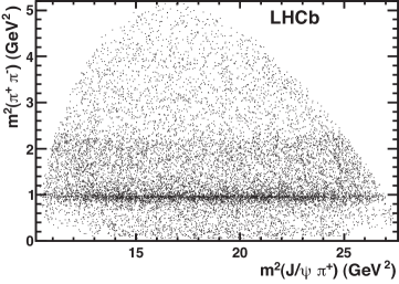
(a) (b)

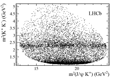
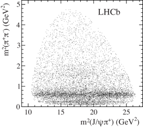
(c) (d)

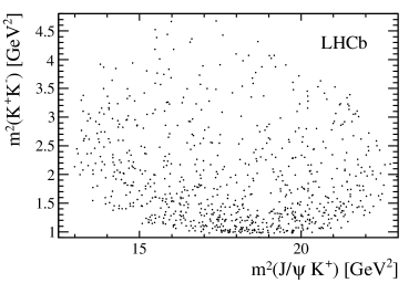
Figure 3: Invariant mass-squared distributions of $h^{+}h^{-}$ vs. $J/\psi h^{+}$ for the decays (a) $\kern 1.79993pt\overline{\kern-1.79993ptB}{}^{0}_{s}\to J/\psi\pi^{+}\pi^{-}$, (b) $\kern 1.79993pt\overline{\kern-1.79993ptB}{}^{0}_{s}\to J/\psi K^{+}K^{-}$, (c) $\kern 1.79993pt\overline{\kern-1.79993ptB}{}^{0}\to J/\psi\pi^{+}\pi^{-}$, and (d) $\kern 1.79993pt\overline{\kern-1.79993ptB}{}^{0}\to J/\psi K^{+}K^{-}$. Note that in this figure we use mass units where we have defined $c=1$.

In these analyses, we apply a formalism similar to that used in Belle’s analysis of $\kern 1.79993pt\overline{\kern-1.79993ptB}{}^{0}\rightarrow K^{-}\pi^{+}\chi_{c1}$ decays [39]. The decay of $\kern 1.79993pt\overline{\kern-1.79993ptB}{}^{0}_{(s)}\to J/\psi h^{+}h^{-}$, where $J/\psi\rightarrow\mu^{+}\mu^{-}$, can be described by four variables. We choose the invariant mass squared of $J/\psi h^{+}$ ($m^{2}(J/\psi h^{+})$), the invariant mass squared of $h^{+}h^{-}$ ($m^{2}(h^{+}h^{-})$), the $J/\psi$ helicity angle ($\theta_{J/\psi}$), and the angle between the $J/\psi$ and $h^{+}h^{-}$ decay planes ($\chi$) in the $\kern 1.79993pt\overline{\kern-1.79993ptB}{}^{0}_{(s)}$ rest frame. The $\chi$ distribution has little structure, so we analyze the decay process after integrating over $\chi$, which eliminates several interference terms. The $m^{2}(h^{+}h^{-})$ vs. $m^{2}(J/\psi h^{+})$ distributions are shown for the $\kern 1.79993pt\overline{\kern-1.79993ptB}{}^{0}_{(s)}\to J/\psi\pi^{+}\pi^{-}$ and $\kern 1.79993pt\overline{\kern-1.79993ptB}{}^{0}_{(s)}\to J/\psi K^{+}K^{-}$ decays in Fig. 3. We model the decay with a series of resonant and non-resonant amplitudes. The data are then fitted with the coherent sum of these amplitudes. Detailed results of all $\kern 1.79993pt\overline{\kern-1.79993ptB}{}^{0}_{(s)}\to J/\psi h^{+}h^{-}$ modified Dalitz plot analyses are available in Refs. [29, 30, 31, 32]. The $\pi^{+}\pi^{-}$ system in $\kern 1.79993pt\overline{\kern-1.79993ptB}{}^{0}_{s}\to J/\psi\pi^{+}\pi^{-}$ is shown to be dominantly in an S-wave state, and the CP-odd fraction in this $\kern 1.79993pt\overline{\kern-1.79993ptB}{}^{0}_{s}$ decay is shown to be greater than 0.977 at 95% confidence level, meaning that $\kern 1.79993pt\overline{\kern-1.79993ptB}{}^{0}_{s}\to J/\psi\pi^{+}\pi^{-}$ decays can be used for studies of mixing-induced CP violation in a large $\pi\pi$ invariant-mass range. In addition, we report the first measurement of the $\kern 1.79993pt\overline{\kern-1.79993ptB}{}^{0}_{s}\to J/\psi\pi^{+}\pi^{-}$ branching fraction relative to $\kern 1.79993pt\overline{\kern-1.79993ptB}{}^{0}_{s}\to J/\psi\phi$ as $(19.79\pm 0.47\pm 0.52)$%, where the first uncertainty is statistical and the second is systematic. We also report the first observation of the $\kern 1.79993pt\overline{\kern-1.79993ptB}{}^{0}\to J/\psi K^{+}K^{-}$ decay. The branching fraction is determined to be $\mathcal{B}(\kern 1.79993pt\overline{\kern-1.79993ptB}{}^{0}\to J/\psi K^{+}K^{-})=(2.53\pm 0.31\pm 0.19)\times 10^{-6}.$ We also set an upper limit of $\mathcal{B}(\kern 1.79993pt\overline{\kern-1.79993ptB}{}^{0}\to J/\psi\phi)<1.9\times 10^{-7}$ at the 90% CL, an improvement of about a factor of five with respect to the previous best measurement [40].

ACKNOWLEDGEMENTS

We express our gratitude to our colleagues in the CERN accelerator departments for the excellent performance of the LHC. We thank the technical and administrative staff at the LHCb institutes. We acknowledge support from CERN and from the national agencies: CAPES, CNPq, FAPERJ and FINEP (Brazil); NSFC (China); CNRS/IN2P3 and Region Auvergne (France); BMBF, DFG, HGF and MPG (Germany); SFI (Ireland); INFN (Italy); FOM and NWO (The Netherlands); SCSR (Poland); MEN/IFA (Romania); MinES, Rosatom, RFBR and NRC “Kurchatov Institute” (Russia); MinECo, XuntaGal and GENCAT (Spain); SNSF and SER (Switzerland); NAS Ukraine (Ukraine); STFC (United Kingdom); NSF (USA). We also acknowledge the support received from the ERC under FP7. The Tier1 computing centres are supported by IN2P3 (France), KIT and BMBF (Germany), INFN (Italy), NWO and SURF (The Netherlands), PIC (Spain), GridPP (United Kingdom). We are thankful for the computing resources put at our disposal by Yandex LLC (Russia), as well as to the communities behind the multiple open source software packages that we depend on.

References

- [1] A. A. Alves Jr. et. al. (LHCb Collaboration), JINST, 3, S08005 (2008).
- [2] R. Aaij et. al., JINST, 8, P04022 (2013).
- [3] R. Aaij et. al. (LHCb Collaboration), Phys. Rev. Lett. 110, 222001 (2013).
- [4] S.-K. Choi et al. (Belle collaboration), Phys. Rev. Lett. 91, 262001 (2003).
- [5] D. Acosta et al. (CDF collaboration), Phys. Rev. Lett. 93, 072001 (2004).
- [6] V. M. Abazov et al. (D0 collaboration ), Phys. Rev. Lett. 93, 162002 (2004).
- [7] B. Aubert et al. (BaBar collaboration), Phys. Rev. D71, 071103 (2005).
- [8] LHCb collaboration, R. Aaij et al., Eur. Phys. J. C72, 1972 (2012).
- [9] CMS collaboration, S. Chatrchyan et al., JHEP 04, 154 (2013).
- [10] N. A. Tornqvist, Phys. Lett. B590, 209 (2004).
- [11] L. Maiani, F. Piccinini, A. D. Polosa, and V. Riquer, Phys. Rev. D71, 014028 (2005).
- [12] C. Hanhart, Y. Kalashnikova, and A. Nefediev, Eur. Phys. J. A47, 101 (2011).
- [13] A. Abulencia et al. (CDF collaboration), Phys. Rev. Lett. 98, 132002 (2007).
- [14] M. Jacob and G. Wick, Annals Phys. 7, 404 (1959).
- [15] J. D. Richman, An experimenter’s guide to the helicity formalism, CALT-68-1148 (ExperimentersGuideToTheHelicityFormalism.pdf, available at http://charm.physics.ucsb.edu/people/richman/) (1984).
- [16] S. U. Chung, Phys. Rev. D57, 431 (1998).
- [17] S.-K. Choi et al. (Belle collaboration), Phys. Rev. D84, 052004 (2011).
- [18] P. del Amo Sanchez et al. (BaBar collaboration), Phys. Rev. D82, 011101 (2010).
- [19] F. James, Statistical methods in experimental physics, World Scientific Publishing, 2006.
- [20] M. Pivk and F. R. Le Diberder, Nucl. Instrum. Meth. A555 356 (2005).
- [21] R. Aaij et. al. (LHCb Collaboration), Euro. Phys. Journal C73, 2462 (2013).
- [22] N. Brambilla et al., Eur. Phys. J. C71 1534 (2011).
- [23] J. S. Lange et al., AIP Conf. Proc. 1374 549 (2011).
- [24] BaBar collaboration, B. Aubert et al., Phys. Rev. D72, (2005) 051101
- [25] Belle collaboration, J. Wei et al., Phys. Lett. B659, (2008) 80.
- [26] J. Beringer et al. (Particle Data Group), Phys. Rev. D86 010001 (2012).
- [27] G. Chen and J. Ma, Phys. Rev. D77 097501 (2008).
- [28] E. Braaten, Phys. Rev. D77 034019 (2008).
- [29] R. Aaij et. al. (LHCb Collaboration), Phys. Rev. D86, 052006 (2012).
- [30] R. Aaij et. al. (LHCb Collaboration), Phys. Rev. D87, 072004 (2013).
- [31] R. Aaij et. al. (LHCb Collaboration), Phys. Rev. D87, 052001 (2013).
- [32] R. Aaij et. al. (LHCb Collaboration), Phys. Rev. D88, 072005 (2013).
- [33] R. Aaij et. al. (LHCb Collaboration), Phys. Lett. B698, 115 (2011).
- [34] J. Li et al. (Belle collaboration), Phys. Rev. Lett. 106, 121802 (2011).
- [35] R. Aaij et al. (LHCb collaboration), Phys. Lett. B707 497 (2012).
- [36] R. Aaij et al. (LHCb collaboration), Phys. Rev. Lett. 108 101803 (2012).
- [37] T. Aaltonen et al. (CDF collaboration), Phys. Rev. D85, 072002 (2012).
- [38] R. Dalitz, Phil. Mag. 44 1068 (1953).
- [39] R. Mizuk et al. (Belle collabration), Phys. Rev. D78 072004 (2008).
- [40] Y. Liu et al. (Belle collaboration), Phys. Rev. D78 011106 (2008).