Thermoelectric efficiency in momentum-conserving systems

Abstract

We show that for a two-dimensional gas of elastically interacting particles the thermoelectric efficiency reaches the Carnot efficiency in the thermodynamic limit. Numerical simulations, by means of the multi-particle collision dynamics method, show that this result is robust under perturbations. That is, the thermoelectric figure of merit remains large when momentum conservation is broken by weak noise.

, ,

Keywords: thermodynamic efficiency, thermoelectricity, conservation laws, anomalous transport

1 Introduction

Understanding and controlling the behaviour of out-of-equilibrium systems is one of the major challenges of modern statistical mechanics. From a fundamental point of view, the challenge is to understand the origin of macroscopic transport phenomenological laws, such as diffusion equations, in terms of the properties of microscopic dynamics, typically nonlinear and chaotic [1, 2]. The problem is extremely complex for coupled flows, so far barely studied from the viewpoint of statistical mechanics and dynamical systems [3, 4, 5, 6, 7, 8, 9, 10, 11, 12]. In particular, it is of primary importance for thermoelectric transport [13, 14, 15, 16] to gain a deeper understanding of the microscopic mechanisms leading to a large thermoelectric efficiency; see Ref. [17] for a review on the fundamental aspects of heat to work conversion.

Within linear response, and for time-reversal symmetric systems  both the maximum thermoelectric efficiency and the efficiency at the maximum output power [22, 23, 24, 25, 26] are monotonous growing functions of the so-called figure of merit $ZT=(\sigma S^{2}/\kappa)T$, which is a dimensionless combination of the main transport coefficients of a material, that is, the electric conductivity $\sigma$, the thermal conductivity $\kappa$ and the thermopower (Seebeck coefficient) $S$, and of the absolute temperature $T$. The maximum efficiency reads $\eta_{\rm max}=\eta_{C}\,\frac{\sqrt{ZT+1}-1}{\sqrt{ZT+1}+1}$, where $\eta_{C}$ is the Carnot efficiency, while the efficiency at maximum output power $P_{\rm max}$ is given by $\eta(P_{\rm max})=\frac{\eta_{C}}{2}\frac{ZT}{ZT+2}$. Thermodynamics only imposes $ZT\geq 0$ and $\eta_{\rm max}\to\eta_{C}$, $\eta(P_{\rm max})\to\frac{\eta_{C}}{2}$ when $ZT\to\infty$.

Since the different transport coefficients are interdependent, it is very difficult to find microscopic mechanisms which could provide insights to design materials with large $ZT$. While for non-interacting models it is well understood that energy filtering [27, 28, 29] allows us to reach the Carnot efficiency, very little is known for interacting systems [30]. It has been recently shown [31] that the thermoelectric figure of merit $ZT$ diverges in the thermodynamic limit for systems with a single relevant conserved quantity, an important example being that of momentum-conserving systems, with total momentum being the only relevant constant of motion. While the mechanism is generic, it has been illustrated in Ref. [31] only for a toy model, i.e., a diatomic chain of hard-point elastically colliding particles.

In this paper, we show by means of extensive multi-particle collision dynamics simulations that the momentum-conservation mechanism leads to the Carnot efficiency in the thermodynamic limit also in the more realistic case of two-dimensional elastically colliding particles. Furthermore, we show that this mechanism leads to a significant enhancement of the thermoelectric figure of merit even when the momentum conservation is not exact due to the existence of an external noise. This robustness is particularly relevant in experiments for which inelastic or incoherent processes are unavoidable to some extent. In this case, the figure of merit saturates with the size of the system to a value higher, the weaker is the noise. Finally, we discuss the validity range of linear response.

The paper is organised as follows. In Sec. 2, in order to make the paper self-contained, we review the theoretical argument of Ref. [31] explaining the divergence of the thermoelectric figure of merit $ZT$ in the thermodynamic limit for systems with a single relevant constant of motion. In Sec. 3 we explain our out-of equilibrium multi-particle collision dynamics simulations. Our numerical results are presented in Sec. 4. We finish with concluding remarks in Sec. 5.

2 Theoretical argument

2.1 Linear response irreversible thermodynamics

The equations connecting fluxes and thermodynamic forces within linear irreversible thermodynamics read as follows [32, 33]:

$$\left(\begin{array}[]{c}J_{\rho}\\ J_{u}\end{array}\right)=\left(\begin{array}[]{cc}L_{\rho\rho}&L_{\rho u}\\ L_{u\rho}&L_{uu}\end{array}\right)\left(\begin{array}[]{c}-\nabla(\beta\mu)\\ \nabla\beta\end{array}\right)\ ,$$ (2.1)

where $J_{\rho}$ and $J_{u}$ are the particle and energy currents, $\mu$ the chemical potential and $\beta=1/T$ the inverse temperature (we set the Boltzmann constant $k_{B}=1$). The kinetic coefficients $L_{ij}$ ( $i,j=\{\rho,u\}$), are related to the familiar transport coefficients as

$$\sigma=\frac{L_{\rho\rho}}{T},\quad\kappa=\frac{1}{T^{2}}\frac{\det{\bm{L}}}{L_{\rho\rho}},\quad S=\frac{1}{T}\left(\frac{L_{\rho u}}{L_{\rho\rho}}-\mu\right),$$ (2.2)

where ${\bm{L}}$ denotes the (Onsager) matrix of kinetic coefficients and we have set the electric charge of each particle $e=1$. Thermodynamics imposes $\det{\bm{L}}\geq 0$, $L_{\rho\rho}\geq 0$, $L_{uu}\geq 0$; $L_{u\rho}=L_{\rho u}$ follows from the Onsager reciprocity relations. The thermoelectric figure of merit reads

$$ZT=\frac{(L_{u\rho}-\mu L_{\rho\rho})^{2}}{\det{\bm{L}}}=\frac{\sigma S^{2}}{\kappa}\,T.$$ (2.3)

Furthermore, the Green-Kubo formula expresses the kinetic coefficients in terms of correlation functions of the corresponding current operators, calculated at thermodynamic equilibrium [34, 35]:

$$L_{ij}=\lim_{\omega\to 0}{\rm Re}L_{ij}(\omega),$$ (2.4)

where

$$L_{ij}(\omega)\equiv\lim_{\epsilon\to 0}\int_{0}^{\infty}dte^{-i(\omega-i\epsilon)t}\lim_{\Omega\to\infty}\frac{1}{\Omega}\int_{0}^{\beta}d\tau\langle{J}_{i}{J}_{j}(t+i\tau)\rangle,$$ (2.5)

where $\langle\;\cdot\;\rangle=\left\{{\rm tr}\left[(\;\cdot\;)\exp^{-\beta H}\right]\right\}/{\rm tr}\left[\exp(-\beta H)\right]$ denotes the equilibrium expectation value at temperature $T$ and $\Omega$ is the system’s volume. Within the framework of Kubo’s linear response approach, the real part of $L_{ij}(\omega)$ can be decomposed into a singular contribution at zero frequency and a regular part $L_{ij}^{\rm reg}(\omega)$ as

$${\rm Re}L_{ij}(\omega)=2\pi{\cal D}_{ij}\delta(\omega)+L_{ij}^{\rm reg}(\omega)\ .$$ (2.6)

The coefficient of the singular part defines the generalized Drude weights ${\cal D}_{ij}$ , which can be expressed as 

$${\cal D}_{ij}=\lim_{t\to\infty}\lim_{l\to\infty}\frac{1}{2\Omega(l)t}\int_{0}^{t}dt^{\prime}\langle J_{i}(t^{\prime})J_{j}(0)\rangle\ ,$$ (2.7)

where in the volume $\Omega(l)$ we have explicitly written the dependence on the system size $l$ along the direction of the thermodynamic flows. Non-zero Drude weights, ${\cal D}_{ij}\neq 0$, are a signature of ballistic transport [37, 38, 39, 40], namely in the thermodynamic limit the kinetic coefficients $L_{ij}$ scale linearly with the system size $l$. As a consequence, the thermopower $S$ does not scale with $l$.

2.2 Conservation laws

We now discuss the influence of conserved quantities on the figure of merit $ZT$. Making use of Suzuki’s formula [41] for the currents $J_{\rho}$ and $J_{u}$, one can generalize Mazur’s inequality [42] by stating that, for a system of finite size $l$ (along the direction of the flows),

$$C_{ij}(l)\equiv\lim_{t\to\infty}C_{ij}(t)=\lim_{t\to\infty}\frac{1}{t}\int_{0}^{t}dt^{\prime}\langle J_{i}(t^{\prime})J_{j}(0)\rangle=\sum_{n=1}^{M}\frac{\langle J_{i}Q_{n}\rangle\langle J_{j}Q_{n}\rangle}{\langle Q_{n}^{2}\rangle},$$ (2.8)

where for readability, in the right hand side of the equation we have omitted the dependence on $l$. The summation in Eq. (2.8) extends over all the $M$ constants of motion $Q_{n}$, which are orthogonal, $\langle Q_{n}Q_{m}\rangle=\langle Q_{n}^{2}\rangle\delta_{n,m}$, and relevant for the considered flows. That is, $\langle J_{\rho}Q_{n}\rangle\neq 0$ and $\langle J_{u}Q_{n}\rangle\neq 0$.

From Eq. (2.8) one can define the finite-size generalized Drude weights as

$$D_{ij}(l)\equiv\frac{1}{2\Omega(l)}\,C_{ij}(l)\ .$$ (2.9)

Therefore, the presence of relevant conservation laws directly implies that the finite-size generalized Drude weights are different from zero. If the thermodynamic limit $l\to\infty$ can be taken after the long-time limit $t\to\infty$, so that the generalized Drude coefficients can be written as

$${\cal D}_{ij}=\lim_{l\to\infty}D_{ij}(l),\$$ (2.10)

and moreover ${\cal D}_{ij}\neq 0$, then we can conclude that the presence of relevant conservation laws yield non-zero generalized Drude weights, which in turn imply that transport is ballistic. We point out that, in contrast to Eq. (2.10), one should take the thermodynamic limit $l\to\infty$ before the long-time limit $t\to\infty$. While it remains an interesting open problem for which classes of models the two limits commute , numerical evidence suggests that it is possible to commute the limits for the models considered in Ref. [31] and in the present paper.

Let us first consider the case in which there is a single relevant constant of motion, $M=1$. We can see from Suzuki’s formula, Eq. (2.8), that the ballistic contribution to $\det{\bm{L}}$ vanishes, since it is proportional to ${\cal D}_{\rho\rho}{\cal D}_{uu}-{\cal D}_{\rho u}^{2}$, which is zero from (2.8) and (2.10). Hence, $\det{\bm{L}}$ grows only due to the contributions involving the regular part in Eq. (2.6), i.e., slower than $l^{2}$, which in turn imply that the thermal conductivity $\kappa\sim\det{\bm{L}}/L_{\rho\rho}$ grows sub-ballistically. Furthermore, since $\sigma\sim L_{\rho\rho}$ is ballistic and $S\sim l^{0}$, we can conclude that

$$ZT=\frac{\sigma S^{2}T}{\kappa}\propto\frac{l}{k}\ .$$ (2.11)

Thus $ZT$ diverges in the thermodynamic limit $l\to\infty$.

The situation is drastically different if $M>1$, as it would be the case for integrable systems, where typically the number of orthogonal relevant constants of motion equals the number of degrees of freedom. In that case, due to the Schwartz inequality,

$$D_{\rho\rho}D_{uu}-D_{\rho u}^{2}=||{\bm{x}}_{\rho}||^{2}||{\bm{x}}_{u}||^{2}-\langle{\bm{x}}_{\rho},{\bm{x}}_{u}\rangle^{2}\geq 0,$$ (2.12)

where

$${\bm{x}}_{i}=(x_{i1},...,x_{iM})=\frac{1}{\sqrt{2\Omega(l)}}\left(\frac{\langle J_{i}Q_{1}\rangle}{\sqrt{\langle Q_{1}^{2}\rangle}},...,\frac{\langle J_{i}Q_{M}\rangle}{\sqrt{\langle Q_{M}^{2}\rangle}}\right),$$ (2.13)

and $\langle{\bm{x}}_{\rho},{\bm{x}}_{u}\rangle=\sum_{k=1}^{M}x_{\rho k}x_{uk}$. The equality arises only in the exceptional case when the vectors ${\bm{x}}_{\rho}$ and ${\bm{x}}_{u}$ are parallel. Hence, for $M>1$ we expect, in general, $\det{\bm{L}}\propto l^{2}$, so that heat transport is ballistic and $ZT\sim l^{0}$.

3 Momentum-conserving gas of interacting particles

In this section we analyse the consequences of our analytical results in a two-dimensional gas of interacting particles. We consider a gas of point-wise particles in a rectangular two-dimensional box of length $l$ and width $w$. The gas container is placed in contact with two particle reservoirs at $x=0$ and $x=l$, through openings of the same size as the width $w$ of the box. In the transversal direction the particles are subject to periodic boundary conditions.

The dynamics of the particles in the system are solved by the method of Multi-particle Collision Dynamics (MPC) [43], introduced as a stochastic model to study solvent dynamics. The MPC simplifies the numerical simulation of interacting particles by coarse graining the time and space at which interactions occurs. MPC correctly captures the hydrodynamic equations [44, 45]. It has been successfully applied to model steady shear flow situations in colloids [46], polymers [47], vesicles in shear flow [48], colloidal rods [49], and more recently to study the steady-state of a gas of particles in a temperature gradient [50].

Under MPC dynamics the system evolves in discrete time steps, consisting on free propagation during a time $\tau$, followed by collision events. During propagation, the coordinates $\vec{r}_{i}$ of each particle are updated as

$$\vec{r}_{i}\rightarrow\vec{r}_{i}+\vec{v}_{i}\tau\ ,$$ (3.1)

where $\vec{v}_{i}$ is the particle’s velocity. For the collisions the system’s volume is partitioned in identical cells of linear size $a$. Then, the velocities of the $\mathcal{N}$ particles found in the same cell are rotated with respect to the center of mass velocity by a random angle. In two dimensions, rotations by an angle $+\alpha$ or $-\alpha$ with equal probability $p(+\alpha)=p(-\alpha)=1/2$ are performed. The velocity updating after a collision event reads

$$\vec{v}_{i}\rightarrow\vec{V}_{\mathrm{CM}}+\hat{\mathcal{R}}^{\pm\alpha}\left(\vec{v}_{i}-\vec{V}_{\mathrm{CM}}\right)\ ,$$ (3.2)

where $\vec{V}_{\mathrm{CM}}=\frac{1}{\mathcal{N}}\sum_{i=1}^{\mathcal{N}}\vec{v}_{i}$ is the center of mass velocity and $\hat{\mathcal{R}}^{\theta}$ is the two-dimensional rotation operator of angle $\theta$. Furthermore, to guarantee Galilean invariance, the collision grid is shifted randomly before each collision step. It has been shown that for these dynamics, the equation of state of the gas of particles corresponds to that of an ideal gas [43]. Moreover, the time interval between successive collisions $\tau$ and the collision angle $\alpha$ tune the strength of the interactions and consequently affects the transport coefficients of the gas of particles. When $\alpha$ is a multiple of $2\pi$, the particles do not interact, propagating ballistically from one reservoir to the other as they cross the system. For any other value of $\alpha$, the particles interact, exchanging momentum during the collision events. The value $\alpha=\pi/2$ corresponds to the most efficient mixing of the particle momenta. Note that by construction, the collision preserve the total energy and total momentum of the gas of particles.

From the reservoir $k$ ($k=L,R$ for the left and the right reservoir), particles of mass $m$ enter the system at rate $\gamma_{k}$ obtained by integration of the appropriate canonical distribution to give

$$\gamma_{k}\ =\ \frac{w}{\left(2\pi m\right)^{1/2}}\rho_{k}T_{k}^{1/2}\ ,$$ (3.3)

where $\rho_{k}$ and $T_{k}$ are the particle density temperature. Assuming that the particles in the reservoirs behave as ideal gas, the particle injection rate is related to the value of the chemical potential $\mu_{k}$ of the reservoir $k$ as

$$\mu_{k}=T_{k}\ln\left(\frac{\gamma_{k}}{T_{k}^{3/2}}\right)+\mu_{0}\ ,$$ (3.4)

with $\mu_{0}$ an arbitrary constant whose value does not qualitatively modify the results discussed in this paper; hereafter we set $\mu_{0}$ in such a way that $\mu=0$ . Whenever a particle from the system crosses the boundary which separates the system from reservoir $k$, it is removed (absorbed in the reservoir), i.e., it has no further effects on the evolution of the system.

4 Discussion of numerical results

We have numerically studied the nonequilibrium transport of the model defined in Sec. 3, coupled to two ideal particle reservoirs. The nonequilibrium state is imposed by setting the values of $T$ and $\mu/T$ in the reservoirs to different values, meaning that from each of the reservoirs, the particles are injected into the system at different rates and with a different distribution of their velocities. Out of equilibrium the kinetic coefficients $L_{ij}$ can be computed, in the linear response regime, by direct measurement of the particle and energy currents in the system. Using (2.1), it is enough to perform two nonequilibrium numerical simulations: one with $T_{L}\neq T_{R}$ and $\mu_{L}/T_{L}=\mu_{R}/T_{R}$, and one with $T_{L}=T_{R}$ and $\mu_{L}/T_{L}\neq\mu_{R}/T_{R}$. In the first simulation the reservoirs’ temperatures are set to $T_{L}=T-\Delta T/2$ and $T_{R}=T+\Delta T/2$, so that the temperature gradient is given by $\Delta T/l$, while $\mu_{L}/T_{L}=\mu_{R}/T_{R}$. Conversely, in the second simulation we set $T_{L}=T_{R}=T$ and using (3.4), we set the particle injection rates $\gamma_{L}$ and $\gamma_{R}$ so that $\Delta\left({\mu}/{T}\right)=\mu_{L}/T_{L}-\mu_{R}/T_{R}=(\mu_{L}-\mu_{R})/T$.

In all simulations the mean particle density and mean temperature in the reservoirs was set to $n=N/lw=22.75$ ($N$ is the mean number of particles) and $T=1$, respectively. We parametrize the gradients in terms of a single parameter by setting, $\Delta T=\Delta\left({\mu}/{T}\right)\equiv\Delta$ (in units where $k_{B}=e=1$). The rotation angle for the collisions in the MPC scheme was set to $\alpha=\pi/2$, unless otherwise specified. The length of the collision cells in the MPC scheme was set to $a=0.1$ and the time step to $\tau=0.25$. For these values and small $\Delta$ the system exhibits reasonably linear temperature and chemical potential profiles in the bulk, with some nonlinear boundary layer near the contacts, arising from the fact that the mean free path of the particles near the boundaries is different than in the bulk , yielding a contact resistance [50]. We performed numerical simulations with up to $\Omega=10^{3}$ ($l=500$ and $w=2$), so that systems with mean number of particles up to $N=4.55\times 10^{4}$ were considered.

4.1 Linear response transport

Using the Suzuki’s formula (2.8), the current-current correlation functions $C_{ij}(t)$ can be obtained analytically. The particle current is $J_{\rho}=\sum_{i=1}^{N}v_{x,i}$ and the energy current $J_{u}=\frac{1}{2}\,m\sum_{i=1}^{N}\left(v_{x,i}^{2}+v_{y,i}^{2}\right)v_{x,i}$ where the coordinate $x$ corresponds to the direction of the thermodynamic gradients, thus the direction of the flows.

Furthermore, for the MPC model there exists a single relevant constant of motion, namely the $x$-component of the total momentum $Q_{1}=p_{x}=m\sum_{i=1}^{N}v_{x,i}$. The other constants of motion, i.e. momentum in the transverse direction, energy and number of particles, are irrelevant since they are orthogonal to the considered flows. Therefore, in this case $M=1$.

Applying Eq. (2.8) and integrating over the equilibrium state at temperature $T$ and fixed number of particles $N$, we obtain that the finite-size correlators are

$$C_{\rho\rho}(l)=\frac{NT}{m}\ ,\quad C_{\rho u}(l)=\frac{2NT^{2}}{m}\ ,\ \mathrm{and}\quad C_{uu}(l)=\frac{4NT^{3}}{m}\ .$$ (4.1)

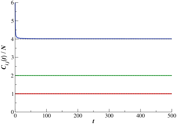
Figure 1: Equilibrium current-current correlation functions. From bottom to top: $C_{\rho\rho}(t)$ (in red), $C_{\rho u}(t)$ (in green) and $C_{uu}(t)$ (in blue), averaged over the ensemble of realisations. The dashed horizontal lines indicate their corresponding analytical values from Eq. (4.1).

To verify Eq. (2.8) we have numerically computed the equilibrium current-current time correlation functions for the isolated system, averaged over an equilibrium ensemble of initial conditions with $N=1000$ particles of mass $m=1$ and temperature $T=1$. A square container of size $l=2$ and periodic boundary conditions in both directions was considered. The results, shown in Fig. 1, verify our the analytical expressions. Note that the initial values $C_{\rho\rho}(0)$ and $C_{\rho u}(0)$ of the time-averaged correlation functions $C_{\rho\rho}(t)$ and $C_{\rho u}(t)$ are equal to their asymptotic values $C_{\rho\rho}(l)=\lim_{t\to\infty}C_{\rho\rho}(t)$ and $C_{\rho u}(l)=\lim_{t\to\infty}C_{\rho u}(t)$. On the other hand, it is easy to compute analytically $C_{uu}(0)=6NT^{3}/m$, and numerical data show that $C_{uu}(t)$ converges algebraically to its asymptotic value $C_{uu}(l)=\lim_{t\to\infty}C_{uu}(t)=4NT^{3}/m$. This asymptotic behaviour may be due to the slow decay of the energy hydrodynamic modes.

Equation (4.1) also shows that the dependence of the correlations on the size $l$ comes exclusively through the number of particles $N$. The thermodynamic limit requires keeping the density of particles fixed, so that the number of particles has to scale linearly with the volume of the system: $N\propto\Omega(l)=lw$. Therefore, Eqs. (4.1) imply that the finite-size generalized Drude weights of Eq. (2.9) do not scale with $l$. Using Eqs. (2.8)-(2.10) we obtain, for fixed $w$, the generalized Drude weights

$${\cal D}_{\rho\rho}=\frac{nT}{2m}\ ,\quad{\cal D}_{\rho u}={\cal D}_{u\rho}=\frac{nT^{2}}{m}\ ,\ \mathrm{and}\quad{\cal D}_{uu}=\frac{2nT^{3}}{m}\ .$$ (4.2)

As a consequence of the finiteness of the Drude weights, the transport is ballistic, meaning that all kinetic coefficients $L_{ij}$ scale linearly with the size of the system: $L_{ij}\sim l$. This prediction is confirmed by the numerical results shown in panel $a$ of Fig. 2.

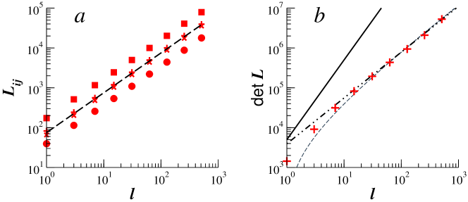
Figure 2: Dependence of the kinetic coefficients on the length of the system $l$, obtained from nonequilibrium simulations with $\Delta=0.00625$. In panel a we show the kinetic coefficients $L_{\rho\rho}$ (circles), $L_{u\rho}$ (crosses), $L_{\rho u}$ (pluses) and $L_{uu}$ (squares). The dashed line stands for the linear scaling $\sim l$. In panel b we plot the determinant of the Onsager matrix $L$ (symbols), as a function of the length of the system. The different curves correspond to the scalings $\sim l^{2}$ (solid), $\sim l\log(l)$ (dashed) and $\sim l^{1.15}$ (dotted-dashed). Parameter values: $m=1$, $T=1$, $n=22.75$, $\alpha=\pi/2$, $w=2$, $a=0.1$, $\tau=0.25$.

More importantly, as discussed in Sec. 2.2, due to the conservation of total momentum, the ballistic contribution to the determinant of the Onsager matrix is zero. Indeed, it can be readily seen from Eq. (4.2) that ${\cal D}_{\rho\rho}{\cal D}_{uu}-{\cal D}_{\rho u}^{2}=0$. Hence a scaling $\det({\bm{L}})$ slower than $l^{2}$ is expected. From the nonequilibrium numerical simulations the scaling of the determinant with $l$ is consistent with $\det({\bm{L}})\approx l^{1.15}$ (dotted-dashed curve in Fig. 2-$b$). It is worthwhile recalling that different analytical methods such as mode coupling theory and hydrodynamics predict, for momentum conserving systems in two dimensions, a logarithmic divergence of the thermal conductivity with the size of the system [1, 2]. Therefore, one should expect that $\det({\bm{L}})\sim l\log(l)$. We show in Fig. 2-$b$ (dashed curve), that such scaling is also consistent with our numerical results, though deviations are larger than for the algebraic behaviour at small system sizes. Since we have no reason to expect an algebraic sub-ballistic behaviour of the heat conductivity, we will assume in what follows that its behaviour is logarithmic.

4.2 Strong enhancement of $ZT$

From Eqs. (2.2) and Eqs. (4.2) we obtain that the electric conductivity also scales linearly with the size of the system:

$$\sigma=\frac{An}{m}\,l\ ,$$ (4.3)

with $A$ constant. The dependence on $l$ of the Seebeck coefficient cancels out to give, asymptotically in $l$,

$$S=\frac{1}{T}\left(\frac{{\cal D}_{\rho u}}{{\cal D}_{\rho\rho}}-\mu\right)=2\ .$$ (4.4)

Since the ballistic contribution to $\det({\bm{L}})$ vanishes, i.e. ${\cal D}_{\rho\rho}{\cal D}_{uu}-{\cal D}_{\rho u}^{2}=0$, we cannot derive an explicit expression for the heat conductivity $\kappa$. However, as discussed in the previous section, for momentum conserving two-dimensional systems it is predicted that $\kappa$ diverges logarithmically with respect to the size of the system: $\kappa\sim\log(l)$.

Fig. 3 shows the dependence of the transport coefficients on the size of the system, for different values of the thermodynamic forces. The electric conductivity verifies Eq. (4.3) independently of the value of the thermodynamic force $\Delta$, with the constant $A=\pi/4$. Instead, the Seebeck coefficient shows a clear dependence on $\Delta$, verifying Eq. (4.4) (asymptotically in $l$) only in the limit of small forces (in Fig. 3, $S$ is shown for $\mu=0$). We have found that $S$ converges to the value $S=2$ predicted by (4.4) as $1/\Delta$.

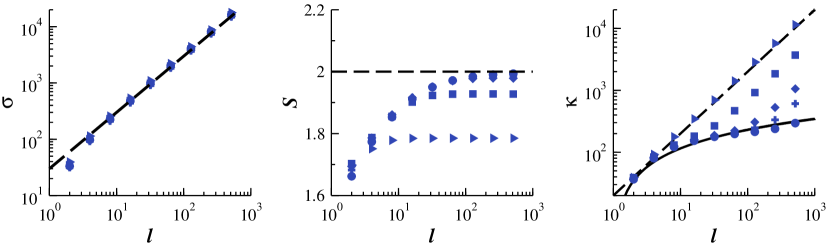
Figure 3: Transport coefficients as a function o the length of the system $l$, for different thermodynamic gradients, $\Delta=0.00625$ (circles), $0.0125$ (pluses), $0.025$ (diamonds), $0.1$ (squares) and $0.4$ (triangles) and the values of other parameters as in the caption of Fig. 2. In panel a the dashed line corresponds to Eq. (4.3) with $A=\pi/4$ and in panel b to $S=2$. In panel c the dashed line stands for linear scaling $\sim l$, while the solid line corresponds to $\log(l)$.

The heat conductivity $\kappa$ exhibits the logarithmic behaviour up to a size $l=l^{\star}$ dependent on the strength $\Delta$ of the thermodynamic forces. For any value of $\Delta$, the heat conductivity grows as $\kappa\sim\log(l)$, for $l>l^{\star}$. The smaller the $\Delta$ the larger the range of validity of the logarithmic $\kappa$ is. We have obtained numerically that the characteristic length $l^{\star}$ grows linearly with $1/\Delta$.

Through Eq. (2.3), this characteristic length $l^{\star}$ does also determine the behaviour of the figure of merit $ZT$. In Fig. 4 we show $ZT$ as a function of $l$, for different values of $\Delta$. We observe that for any value of $\Delta$, $ZT$ is in reasonable agreement with an initial grow $l/\log(l)$ for $l<l^{\star}$ and for larger sizes saturates to a maximum value $(ZT)_{\mathrm{max}}$. Our results show that as a consequence of the existence of a single relevant conserved quantity, the values of $ZT$ are greatly enhanced when the system under consideration is large enough. Moreover, $ZT$ does not grow unboundedly, but reaches a maximum value that grows with $\approx(1/\Delta)^{0.9}$ (see the inset of Fig. 4). The deviations at short sizes are probably due to the slow convergence of the Seebeck coefficient to its asymptotic value $2$.

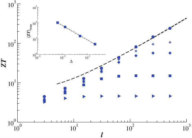
Figure 4: Thermoelectric figure-of-merit $ZT$ as a function of the length of the system $l$ for different thermodynamic gradients, $\Delta=0.00625$ (circles), $0.0125$ (pluses), $0.025$ (diamonds), $0.1$ (squares) and $0.4$ (triangles) and the other parameter values as in the caption of Fig. 2. The dashed curve stands for $\sim l/\log(l)$ In the inset, we show the maximum (saturation) value of $ZT$ as a function of $\Delta$. The dashed line is a power-law fit, $(ZT)_{\rm max}=\Delta^{\alpha}$, with $\alpha\approx-0.9$.

Figure 5: Figure-of-merit $ZT$ as a function of the length of the system $l$, for different values of the collision parameter $\alpha$, for $\Delta=0.1$, and from bottom to top: $\alpha=0$, $1/5$, $1/2$, $\pi/4$ and $\pi/2$. The other parameter values are as in Fig. 2.

In the above discussion on the behaviour of the transport coefficients and the figure of merit $ZT$ as a function of $\Delta$, we should keep in mind that such coefficients and consequently also $ZT$ are defined in the linear response regime, i.e. in the limit of small thermodynamic forces, formally for $\Delta\to 0$. On the other hand, we numerically computed the kinetic coefficients, for any given $\Delta$, via the fluxes as discussed at the beginning of Sec. 4. That is to say, there is no saturation of $ZT$ within linear response. On the other hand, the numerically observed saturation (as well as the ballistic behaviour of $\kappa$ for $l>l^{\star}$) signals that the range of linear response shrinks with the system size when computing $\kappa$ and $ZT$. At first sight, this failure of linear response for a given $\Delta$ and large $l$ appears counterintuitive, since for fixed $\Delta$ larger $l$ means smaller thermodynamic forces, and it is in the limit of small forces that linear response is expected to be valid. There is actually no such problem when computing the kinetic coefficients $L_{ij}$. As shown in Fig. 3 for the charge conductivity $\sigma=L_{\rho\rho}/T$, data at different $\Delta$ collapse on a single curve, showing that for all values of $\Delta$ in that figure we are within linear response. The problem arises when considering non-trivial combinations of the kinetic coefficients, as in $\kappa\propto\det({\bm{L}})$ and consequently in $ZT$. Our theory predicts the divergence of $ZT$ in the thermodynamic limit and $ZT$ diverges (thus leading to Carnot efficiency) if and only if the Onsager matrix $L$ becomes ill-conditioned, namely the condition number $[\Tr({\bm{L}})]^{2}/\det({\bm{L}})$ diverges (in our model as $l/\log(l)$) and therefore the system (2.1) becomes singular. That is, the charge and energy currents become proportional, a condition commonly referred to as strong coupling, i.e. $J_{\rho}=cJ_{u}$, the proportionality factor $c$ being independent of the applied thermodynamic forces. The Carnot efficiency is obtained in such singular limit and it is in attaining such limit that the validity range of linear response shrinks. Therefore, as expected on general grounds, the Carnot efficiency is obtained only in the limit of zero forces and zero currents, corresponding to reversible transport (zero entropy production) and zero output power.

It is worthwhile noticing that for our model in the non-interacting limit the momentum of each particle is conserved, meaning that the system is integrable and the number of conserved observables $M\propto l$, thus diverging in the thermodynamic limit. As we have discussed at the end of section 2.2, one expects that in such integrable situation, $ZT$ does not scale with the system size. To corroborate this expectation we show in Fig. 5 the dependence of $ZT$ on $l$ for different values of the collisional parameter $\alpha$. We recall that at the collisions, $\alpha=\pi/2$ corresponds to the most efficient mixing of the particle momenta, while $\alpha=0$ corresponds to no interaction. As expected, for the non-interacting gas, namely for an infinite number of conserved quantities, $ZT$ does not scale with $l$, attaining the value $3/2$ characteristic of a two-dimensional ideal gas [7]. The enhancement of $ZT$ is observed for any value of $\alpha>0$, as then only the total momentum is preserved and $M=1$. Our data also suggest a rather weak dependence of $(ZT)_{\mathrm{max}}$ on $\alpha$.

4.3 Systems with noise

The results discussed above show the enhancement of $ZT$, and thus of the thermoelectric efficiency, in systems with conserved total momentum. In real systems, however, total momentum is never conserved due to the phonon field, the presence of impurities or in general to inelastic scattering events.

In this section we want to explore to what extent the break down of total moment conservation modifies the results obtained above. To address this question numerically, we consider the existence of a source of stochastic noise. From a physical point of view, this noise source may model the interactions of the gas with the walls of the container, or the inelastic scattering from impurities in the material. We model the stochastic noise as follows: after a collision of the particles in a given cell has taken place, with probability $\varepsilon$ the velocities of all the particles in the cell are reflected, namely $\vec{v}_{i}\rightarrow-\vec{v}_{i}$. Therefore for any $\varepsilon>0$ the total momentum is not longer conserved. If $\varepsilon$ is small the momentum conservation is weakly broken and we want to investigate how our results depend on the strength $\varepsilon$ of the perturbation.

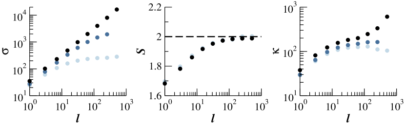
Figure 6: The dependence of the transport coefficients on the size $l$ of the system, for $\Delta=0.0125$ and different noise intensities: from darker to lighter, $\varepsilon=0$, $0.01$ and $0.1$. The other parameter values are as in Fig. 2.

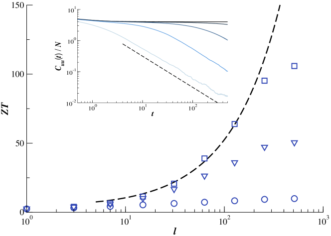
Figure 7: Figure-of-merit $ZT$ as a function of the length of the system $l$, for different noise intensities $\varepsilon=0$ (squares), $0.01$ (triangles) and $0.1$ (circles). The thermodynamic gradient was fixed to $\Delta=0.0125$. The dashed curve corresponds to the expected linear response dependence at $\varepsilon=0$, i.e. $ZT\sim l/\log(l)$. In the inset: energy current-current correlation for different noise intensities $\varepsilon$, for the same parameter values as in Fig. 6. From top to bottom: $\varepsilon=0,10^{-4},10^{-3},10^{-2},10^{-1}$. The dashed curve stands for $\sim 1/t$.

In Fig. 6 we show the dependence of the transport coefficients on $l$ for fixed $\Delta$ and different strengths of the noise $\varepsilon$. We observe that for sufficiently strong noise all transport coefficients appear to become independent of $l$, as expected in a diffusive regime in which total momentum is not preserved.

More interesting is the behaviour of $ZT$ shown in Fig. 7. We see that at stronger noise, $ZT$ becomes constant, as expected in the diffusive regime. From a mathematical point of view, the absence of conserved quantities ($M=0$) leads to decaying correlation functions and zero Drude coefficients (inset of Fig. 7). Thus the transport coefficients and $ZT$ become size-independent.

More importantly, we see that when the convergence toward the diffusive regime is smooth, meaning that when the conservation of total momentum is only weakly perturbed (small $\varepsilon$), the enhancement of $ZT$ can be significant. This shows that the effect described here is robust against perturbations.

5 Conclusions

In summary, we have shown that in two-dimensional interacting systems, with the interactions modeled by the multi-particle collision dynamics method, the thermoelectric figure of merit diverges at the thermodynamic limit. In such limit, the Carnot efficiency is obtained with zero output power. When noise is added to the system, $ZT$ saturates at large $l$, to values higher the weaker is the noise strength.

Our findings could be relevant in situations in which the elastic mean free path is longer than the length scale over which interactions are effective in exchanging momenta between the particles. Suitable conditions to observe the interaction-induced enhancement of the thermoelectric figure of merit might be found in high-mobility two-dimensional electron gases at low temperatures. In such systems very large elastic mean free paths have been reported (for instance, up to $28$ $\mu$m in Ref. [51]). At low temperatures the inelastic mean free path is determined by electron-electron interactions rather than by phonons. It should be therefore possible to find a temperature window where electron-electron interactions dominate, i.e. are effective on a scale smaller than the elastic mean free path and are dominant over phonon effects. It would be, however, highly desirable to test our arguments in such regime, by means of numerical simulations of quantum systems.

References

References

- [1] Lepri S, Livi R and Politi A 2003 Phys. Rep. 377 1.
- [2] Dhar A. 2008 Adv. Phys. 57 457.
- [3] Vollmer J, Tamás T, and Mátyás L 2000 J. Stat. Phys. 101 79.
- [4] Mejía-Monasterio C, Larralde H and Leyvraz F 2001 Phys. Rev. Lett. 86 5417.
- [5] Larralde H, Leyvraz and Mejía-Monasterio C 2003 J. Stat. Phys. 113 197.
- [6] Maes C and van Wieren M H 2005 J. Phys. A 38 1005.
- [7] Casati G, Mejía-Monasterio C and Prosen T 2008 Phys. Rev. Lett. 101 016601.
- [8] Casati G, Wang L and Prosen T 2009 J. Stat. Mech. L03004.
- [9] Wang J, Casati G, Prosen T and Lai C-H 2009 Phys. Rev. E 80 031136.
- [10] Saito K, Benenti G and Casati G 2010 Chem. Phys. 375 508.
- [11] Benenti G and Casati G 2011 Phil. Trans. R. Soc. A 369 466.
- [12] Iubini S, Lepri S and Politi A 2012 Phys. Rev. E 86 011108.
- [13] Dresselhaus M S, Chen G, Tang M Y, Yang R G, Lee H, Wang D Z, Ren Z F, Fleurial J-P and Gogna P 2007 Adv. Mater. 19 1043.
- [14] Snyder G J and Toberer E S 2008 Nature Mater. 7 105.
- [15] Shakouri A 2011 Annu. Rev. Mater. Res. 41 399.
- [16] Dubi Y and Di Ventra M 2011 Rev. Mod. Phys. 83 131.
- [17] Benenti G, Casati G, Prosen T and Saito K preprint arXiv:1311.4430 [cond-mat.stat-mech].
- [18] Benenti G, Saito K and Casati G 2011 Phys. Rev. Lett. 106 230602.
- [19] Brandner K, Saito K and Seifert U 2013 Phys. Rev. Lett. 110 070603.
- [20] Balachandran V, Benenti G and Casati G 2013 Phys. Rev. B 87 165419.
- [21] Brandner K and Seifert U 2013 New J. Phys. 15 105003.
- [22] Van den Broeck C 2005 Phys. Rev. Lett. 95 190602.
- [23] Esposito M, Lindenberg K and Van den Broeck C 2009 Phys. Rev. Lett. 102 130602.
- [24] Gaveau B, Moreau M and Schulman LS 2010 Phys. Rev. Lett. 105 060601.
- [25] Esposito M, Kawai R, Lindenberg K and Van den Broeck C 2010 Phys. Rev. Lett. 105 150603.
- [26] Seifert U 2011 Phys. Rev. Lett. 106 020601.
- [27] Mahan G D and Sofo J O 1996 Proc. Natl. Acad. Sci. USA 93 7436.
- [28] Humphrey T E, Newbury R, Taylor R P and Linke H 2002 Phys. Rev. Lett. 89 116801.
- [29] Humphrey T E and Linke H 2005 Phys. Rev. Lett. 94 096601.
- [30] Casati G and Mejía-Monasterio C 2008 AIP Conference Proceedings, 1076 18.
- [31] Benenti G, Casati G and Wang J 2013 Phys. Rev. Lett. 110 070604.
- [32] Callen H B 1985 Thermodynamics and an Introduction to Thermostatics (second edition) (New York: John Wiley & Sons).
- [33] de Groot S R and Mazur P 1962 Nonequilibrium Thermodynamics (Amsterdam: North-Holland).
- [34] Kubo R, Toda M and Hashitsume N 1985 Statistical Physics II: Nonequilibrium Statistical Mechanics (Springer-Verlag).
- [35] Mahan G D Many-Particle Physics 1990 (New York: Plenum Press).
- [36] Ilievski E and Prosen T 2013 Commun. Math. Phys. 318 809.
- [37] Zotos X, Naef F and Prelovšek P 1997 Phys. Rev. B 55 11029.
- [38] Zotos X and Prelovšek P, in Baeriswyl D and Degiorgi L (Eds.) 2004 Strong Interactions in Low Dimensions (Dordrecht: Kluwer Academic Publishers, Dordrecht).
- [39] Garst M and Rosch A 2001 Europhys. Lett. 55 66.
- [40] Heidrich-Meisner F, Honecker A and Brenig W 2005 Phys. Rev. B 71 184415.
- [41] Suzuki M 1971 Physica 51 277.
- [42] Mazur P 1969 Physica 43 533.
- [43] Malevanets A and Kapral R 1999 J. Chem. Phys. 110 8605.
- [44] Padding J T and Louis A A 2006 Phys. Rev. E 74 031402.
- [45] Gompper G, Ihle T, Kroll D M and Winkler R G 2009 Adv. Polymer S. 221 1.
- [46] Hecht M, Harting J, Bier M, Reinshagen J and Herrmann H J 2006 Phys. Rev. E 74 021403.
- [47] Nikoubashman A and Likos C N 2010, Macromol. 43 1610.
- [48] Noguchi H and Gompper G 2007 Phys. Rev. Lett. 98 128103.
- [49] Ripoll M, Holmqvist P, Winkler R G, Gompper G, Dhont J K G and Lettinga M P 2008 Phys. Rev. Lett. 101 168302.
- [50] Lüsebrink D and Ripoll M 2012 J. Chem. Phys. 136 084106.
- [51] Jura M P, Topinka M A, Urban L, Yazdani A, Shtrikman H, Pfeiffer L N, West K W and Goldhaber-Gordon D 2007 Nature Phys. 3 841.