Event Evolution Tracking from Streaming Social Posts

Abstract

Online social post streams such as Twitter timelines and forum discussions have emerged as important channels for information dissemination. They are noisy, informal, and surge quickly. Real life events, which may happen and evolve every minute, are perceived and circulated in post streams by social users. Intuitively, an event can be viewed as a dense cluster of posts with a life cycle sharing the same descriptive words. There are many previous works on event detection from social streams. However, there has been surprisingly little work on tracking the evolution patterns of events, e.g., birth/death, growth/decay, merge/split, which we address in this paper. To define a tracking scope, we use a sliding time window, where old posts disappear and new posts appear at each moment. Following that, we model a social post stream as an evolving network, where each social post is a node, and edges between posts are constructed when the post similarity is above a threshold. We propose a framework which summarizes the information in the stream within the current time window as a “sketch graph” composed of “core” posts. We develop incremental update algorithms to handle highly dynamic social streams and track event evolution patterns in real time. Moreover, we visualize events as word clouds to aid human perception. Our evaluation on a real data set consisting of 5.2 million posts demonstrates that our method can effectively track event dynamics in the whole life cycle from very large volumes of social streams on the fly.

1 Introduction

In the current social web age, people easily feel overwhelmed by the information deluge coming from post streams which flow in from channels like Twitter, Facebook, forums, Blog websites and email-lists. As of 2009, it was reported [1], e.g., that each Twitter user follows 126 users on average, and on each day, the received social streaming posts will cost users considerable time to read, only to discover a small interesting part. This is a huge overhead that users pay in order to find a small amount of interesting information. There is thus an urgent need to provide users with tools which can automatically extract and summarize significant information from highly dynamic social streams, e.g., report emerging bursty events, or track the evolution of a specific event in a given time span. There are many previous studies [19, 22, 24, 25, 12, 7] on detecting new emerging events from text streams; they serve the need for answering the query “what’s happening?” over social streams. However, in many scenarios, users may want to know more details about an event and may like to issue advanced queries like “how’re things going?”. For example, for the event “SOPA (Stop Online Piracy Act) protest” happening in January 2012, existing event detection approaches can discover bursty activities at each moment, but cannot answer queries like “how SOPA protest has evolved in the past few days?”. An ideal output to such an evolution query would be a “panoramic view” of the event history, which improves user experience. In this work, we consider this kind of queries as an instance of the event evolution tracking problem, which aims to track the event evolutionary dynamics at each moment from social streams. Typical event evolution patterns include emerging (birth) or disappearing (death), inflating (growth) or shrinking (decay), and merging or splitting of events. Event detection can be viewed as a subproblem of event evolution tracking. We try to solve the event evolution tracking problem in the paper.

There are several major challenges in the tracking of event evolution. The first challenge is the effective organization of noisy social post streams into a meaningful structure. Social posts such as tweets are usually written in an informal way, with lots of abbreviations, misspellings and grammatical errors. Even worse, a correctly written post may have no significance and be just noise. Recent works on event detection from Twitter [28, 22] recognize and handle noise in post streams in a limited and ad hoc manner but do not handle noise in a systematic formal framework. The second challenge is how to track and express the event evolution behaviors precisely and incrementally. Most related work reports event activity by volume on the time dimension [22, 19]. While certainly useful, this cannot show the evolution behaviors about how events are split or merged, for instance. The third challenge is the summary and annotation of events. Since an event may easily contain thousands of posts, it is important to summarize and annotate it in order to facilitate human perception. Recent related works [22, 19, 28] typically show users just a list of posts ranked by importance or time freshness, which falls short of addressing this challenge.

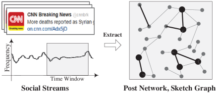
(a) The sketch-based framework

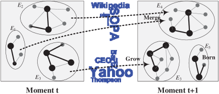
(b) Event evolution tracking

Figure 1: (a) Post network captures the correlation between posts in the time window at each moment, and evolves as time rolls on. Core nodes and core edges are bolded. (b) From moment $t$ to $t+1$, typical event evolution behaviors include birth or death, growth or decay, merging or splitting of events. Each event is annotated by a topical word cloud.

To handle the above mentioned challenges, we first model social streams as an evolving post network, and then propose a sketch graph-based framework to track the evolution of events in the post network (Section 4.1). Intuitively, a sketch graph can be viewed as a compact summary of the original post network. The sketch graph only contains core posts from the post network, where core posts are defined as posts that play a central role in the network. Noise posts will be directly pruned by the sketch graph. As we will discuss in Section 5, evolution behaviors can be effectively and incrementally expressed based on a group of primitive operations in the sketch graph. Technically, we define an event as a cluster in the post network, and then summarize and annotate each event by topical word-clouds. We show an overview of major steps for event tracking from social streams in Figure 1. Note that as time rolls on, the post network, events and their annotations will be updated incrementally at each moment.

We notice that at a high level, our definition seemingly resembles previous work on density-based clustering over streaming data, e.g., DenStream in [9] and cluster maintenance in [2] and [5]. However, there are several major differences. First, our approach works on an evolving graph structure and provides users the flexibility in choosing the scope for tracking and monitoring new events by means of a fading time window, while the existing work doesn’t provide a tracking scope. Second, the existing work can only process the adding of nodes/edges one by one, while our approach can handle adding, deleting and fading of nodes subgraph by subgraph. This is an important requirement for dealing with the high throughput rate of online post streams. Third, the focus of our approach is tracking and analyzing the evolution dynamics in the whole life cycle of events. By contrast, they focus on the maintenance of clusters, which is only a sub-task in our problem.

Finally, to compare with traditional topic tracking on news article streams, we note that this problem is usually formulated as a classification problem [4]: when a new story arrives, compare it with topic features in the training set and if it matches sufficiently, declare it to be on a topic. Commonly used techniques include decision trees and $k$-NN [29]. This approach assumes that topics are predefined before tracking. Thus, we cannot simply apply topic tracking techniques to event tracking in social streams, since future events are unknown and may not conform to any previously known topics. Moreover, traditional topic tracking has difficulties in tracking the composite behaviors such as merging and splitting, which are definitely a key aspect of event evolution.

In summary, the main problem we study in this paper is captured by the following questions: how to efficiently track the evolution behavior of social post streams such as Twitter, which are noisy and highly dynamic? how to do this incrementally? what is an effective way to express evolution behavior of events? In this paper, we develop a framework and algorithms to answer all these questions. Our main contributions are the following:

• We design an effective approach to extract and organize meaningful information from noisy social streams (Section 3);

• We filter noisy posts by introducing sketch graph (Section 4.1)), based on which we define a group of primitive operations and express evolution behaviors with respect to graphs and events using these primitive operations (Section 5);

• We propose efficient algorithms cTrack and eTrack to track the evolution of clusters and events accurately and incrementally, superior in both quality and performance to existing approaches that find the evolution patterns by matching events in consecutive time moments (Section 6).

• Our evaluation on a large real data set demonstrates that our method can effectively track all six kinds of event evolution behaviors from highly dynamic social post streams in a scalable manner (Section 7).

More related work is discussed in Section 2. We summarize the paper and discuss extensions in Section 8. For convenience, we summarize the major notations used in the paper, in Table 1.

$S(p_{1},p_{2})$	the content similarity between $p_{1}$ and $p_{2}$
$S_{F}(p_{1},p_{2})$	the fading similarity between $p_{1}$ and $p_{2}$
$(\delta_{1},\varepsilon_{0},\varepsilon_{1})$	density factors for core post, edge and core edge
$w^{t}(p)$	the weight of post $p$ at time moment $t$
$\mathcal{G}_{t}(\mathcal{V}_{t},\mathcal{E}_{t})$	the post network at moment $t$
$G_{t}(V_{t},E_{t})$	the sketch graph of the post network at moment $t$
$\mathcal{N}(p)$	the neighbor set of $p$ in $\mathcal{G}_{t}$
$\overline{C},\overline{S}_{t}$	a component, a component set at moment $t$
$C,S_{t}$	a cluster, a cluster set at moment $t$
$N_{c}(p)$	the set of clusters where $p$’s neighboring core posts belong
$E,\widetilde{S}_{t}$	an event, an event set at moment $t$
$A$	the annotation for an event

Table 1: Notation.

2 Related Work

Work related to this paper mainly falls in one of these categories.

Topic/Event/Community detection and tracking. Most previous works detect events by discovering topic bursts from a document stream. Their major techniques are either detecting the frequency peaks of event-indicating phrases over time in a histogram, or monitoring the formation of a cluster from a structure perspective. A feature-pivot clustering is proposed in [12] to detect bursty events from text streams. Sarma et al. [25] design efficient algorithms to discover events from a large graph of dynamic relationships. Jin et al. [15] present Topic Initiator Detection (TID) to automatically find which web document initiated the topic on the Web. Louvain method [8], based on modularity optimization, is the state-of-the-art community detection approach which outperforms others. However, Louvain method cannot not resist massive noise. None of the above works address the event evolution tracking problem.

There is less work on evolution tracking. An event-based characterization of behavioral patterns for communities in temporal interaction graphs is presented in [6]. A framework for tracking short, distinctive phrases (called “memes”) that travel relatively intact through on-line text was developed in [19]. Unlike these works, we focus on the tracking of real world event-specific evolution patterns from social streams.

Social Stream Mining. Weng et al. [28] build signals for individual words and apply wavelet analysis on the frequency of words to detect events from Twitter. Twitinfo [22] detects events by keyword peaks and represents an event it discovers from Twitter by a timeline of related tweets. Recently, Agarwal et al. [2] discover events that are unraveling in microblog streams, by modeling events as dense clusters in highly dynamic graphs. Angel et al. [5] study the efficient maintenance of dense subgraphs under streaming edge weight updates. Both [2] and [5] model the social stream as an evolving entity graph, but suffer from the drawback that post attributes like time and author cannot be reflected. Another drawback of [2] and [5] is that they can only handle edge-by-edge updates, but cannot handle subgraph-by-subgraph bulk updates. Both drawbacks are solved in our paper.

Clustering and Evolving Graphs. In this paper, we summarize an original post network into a sketch graph based on density parameters. Compared with partitioning-based approaches (e.g., K-Means [14]) and hierarchical approaches (e.g., BIRCH [14]), density-based clustering (e.g., DBSCAN [14]) is effective in finding arbitrary-shaped clusters, and is robust to noise. The main challenge is to apply density-based clustering on fast evolving post networks. CluStream [3] is a framework that divides the clustering process into an online component which periodically generates detailed summary statistics for nodes and an offline component which uses only the summary statistics for clustering. However, CluStream is based on K-Means only. DenStream [9] presents a new approach for discovering clusters in an evolving data stream by extending DBSCAN. This work is related to us in that both employ density based clustering. The differences between our approach and DenStream were discussed in detail in the introduction. Subsequently, DStream [10] uses an online component which maps each input data record into a grid and an offline component which generates grid clusters based on the density. Another related work is by Kim et al. [16], which first clusters individual snapshots into quasi-cliques and then maps them over time by looking at the density of bipartite graphs between quasi-cliques in adjacent snapshots. Although [16] can handle birth, growth, decay and death of clusters, the splitting and merging behaviors are not supported. In contrast, our approach is totally incremental and is able to track composite behaviors like merging and splitting in real time.

3 Post Network Construction

In this section, we describe how we construct a post network from a social post stream. The main challenge is detecting similarity between streaming posts efficiently and accurately, taking the time of the posts into account. We use a notion of fading similarity (Section 3.2) and propose a technique called linkage search to efficiently detect posts similar to a post as it streams in (Section 3.3).

3.1 Social Stream Preprocessing

Social posts such as tweets are usually written in an informal way. Our aim is to design a processing strategy that can quickly judge what a post talks about and is robust enough to the informal writing style. In particular, we focus on the entity words contained in a post, since entities depict the topic. For example, given a tweet “iPad 3 battery pointing to thinner, lighter tablet?”, the entities are “iPad”, “battery” and “tablet”. However, traditional Named Entity Recognition tools [23] only support a narrow range of entities like Locations, Persons and Organizations. NLP parser based approaches [17] are not appropriate due to the informal writing style of posts and the need for high processing speed. Also, simply treating each post text as a bag of words [21] will lead to loss of accuracy, since different words have different weights in deciding the topic of a post. To broaden the applicability, we treat each noun in the post text as a candidate entity. Technically, we obtain nouns from a post text using a Part-Of-Speech Tagger, and if a noun is plural (POS tag “NNS” or “NNPS”), we obtain the prototype of this noun using WordNet stemmer. In practice, we find this preprocessing technique to be robust and efficient. In the Twitter dataset we used in our experiments (see Section 7), each tweet contains 4.9 entities on an average. We formally define a social post as follows.

Definition 1

(Post). A post $p$ is a triple $(L,\tau,u)$, where $L$ is the list of entities in the post, $\tau$ is the time stamp of the post, and $u$ is the user who posted it.

We let $p^{L}$ denote $L$ in the post $p$ for simplicity, and analogously for $p^{\tau}$ and $p^{u}$. We use $|p^{L}|$ to denote the number of entities in $p$.

3.2 Fading Similarity

Post similarity is the most crucial criterion in correlating posts of the same event together. Traditional similarity measures such as TF-IDF based cosine similarity, Jaccard Coefficient and Pearson Correlation [21] only consider the post content. However, clearly time dimension should play an important role in determining post similarity, since posts created closer together in time are more likely to discuss the same event than posts created at very different moments. We introduce the notion of fading similarity to capture both content similarity and time proximity. Formally, we define the fading similarity between a pair of posts $p_{i}$ and $p_{j}$ as

$$S_{F}(p_{i},p_{j})={S(p_{i}^{L},p_{j}^{L})\over D(|p_{i}^{\tau}-p_{j}^{\tau}|)}\vspace{-0.2cm}$$ (1)

where $S(p_{i}^{L},p_{j}^{L})$ is a set-based similarity measure that maps the similarity between $p_{i}^{L}$ and $p_{j}^{L}$ to the interval $[0,1]$, and $D(|p_{i}^{\tau}-p_{j}^{\tau}|)$ is a distance measure that is monotonically increasing with $|p_{i}^{\tau}-p_{j}^{\tau}|$ and $D(|p_{i}^{\tau}-p_{j}^{\tau}|)\geq 1$. For example, $S(p_{i}^{L},p_{j}^{L})$ may be the Jaccard coefficient with $S(p_{i}^{L},p_{j}^{L})={(|p_{i}^{L}\cap p_{j}^{L}|)}/{(|p_{i}^{L}\cup p_{j}^{L}|)}$, and $D(|p_{i}^{\tau}-p_{j}^{\tau}|)$ may be $D(|p_{i}^{\tau}-p_{j}^{\tau}|)=e^{|p_{i}^{\tau}-p_{j}^{\tau}|}$. We will compare different measures in experiments. It is known that nouns are usually more topic relevant than verbs, adjectives, etc [20]. Consequently, entity-based similarity of posts is more appropriate than similarity based on all words. Besides, it has the advantage of smaller computational overhead. It is trivial to see that $0\leq S_{F}(p_{i},p_{j})\leq 1$ and that $S_{F}(p_{i},p_{j})$ is symmetric.

3.3 Post Network and Linkage Search

To find the implicit correlation between posts as they stream in, we build a post network based on the following rule: if the fading similarity between two posts is higher than a given threshold $\varepsilon_{0}$, we create an edge between them. More formally:

Definition 2

(Post Network). The snapshot of post network at moment $t$ is defined as a graph $\mathcal{G}_{t}(\mathcal{V}_{t},\mathcal{E}_{t})$, where each node $p\in\mathcal{V}_{t}$ is a post, and an edge $(p_{i},p_{j})\in\mathcal{E}_{t}$ is constructed iff $S_{F}(p_{i},p_{j})\geq\varepsilon_{0}$, where $0<\varepsilon_{0}<1$ is a given parameter.

We monitor social streams using a fading time window, which will be introduced explicitly in Section 5.3. For now, imagine a time window of observation and consider the post network at the beginning of the time window. As we move forward in time, new posts flow in and old posts fade out and $\mathcal{G}_{t}(\mathcal{V}_{t},\mathcal{E}_{t})$ is dynamically updated at each moment, with new nodes/edges added and old nodes/edges removed. Removing a node and associated edges from $\mathcal{G}_{t}(\mathcal{V}_{t},\mathcal{E}_{t})$ is an easy operation, so let us investigate the case when a node is added. When a new post $p$ flows in, we need to construct the linkage (i.e., edges) between $p$ and nodes in $\mathcal{V}_{t}$, following Definition 2. In a real scenario, since the number of nodes $|\mathcal{V}_{t}|$ can easily go up to millions, it is impractical to compare $p$ with every node in $\mathcal{V}_{t}$ to verify the satisfaction of Definition 2. Below, we propose Linkage Search to identify the neighbors of $p$ accurately by accessing only a small subset of nodes in $\mathcal{V}_{t}$.

Linkage Search. Let $\mathcal{N}(p)$ denote the set of neighbors of $p$ that satisfy Definition 2. The problem of linkage search is finding $\mathcal{N}(p)$ accurately by accessing only a small node set $\mathcal{N}^{\prime}$, where $\mathcal{N}(p)\subseteq\mathcal{N}^{\prime}\subset\mathcal{V}_{t}$ and $|\mathcal{N}^{\prime}|\ll|\mathcal{V}_{t}|$. To solve this problem, first we construct a post-entity bipartite graph, and then perform a two-step random walk process on this bipartite graph and use the hitting counts. The main idea of linkage search is to let a random surfer start from post node $p$ and walk to any entity node in $p^{L}$ on the first step, and continue to walk back to post nodes except $p$ on the second step. All the post nodes visited on the second step form a set $\mathcal{N}^{\prime}$. For any node $q\in\mathcal{N}^{\prime}$, $q$ can be hit multiple times from different entities and the total hitting count $\mathcal{H}(p,q)$ can be aggregated. Assuming the measure of $S(p^{L},q^{L})$ in Eq. (1) is Jaccard coefficient, we can verify the linkage between $p$ and $q$ by checking the condition

$$S_{F}(p,q)={\mathcal{H}(p,q)\over{\left(|p^{L}|+|q^{L}|-\mathcal{H}(p,q)\right)D(|p^{\tau}-q^{\tau}|)}}\geq\varepsilon_{0}\vspace{-0.2cm}$$ (2)

Linkage search supports the construction of a post network on the fly. It is easy to see that for post $q\not\in\mathcal{N}^{\prime}$, $S_{F}(p,q)=0$. Thus, we do not need to access posts that are not in $\mathcal{N}^{\prime}$. Since a post like tweet usually connects to very few entities, $|\mathcal{N}^{\prime}|\ll|\mathcal{V}_{t}|$ generally holds, thus making linkage search very efficient. Suppose the average number of entities in each post is $d_{1}$ and the average number of posts mentioning each entity is $d_{2}$. Then linkage search can find the neighbor set of a given post in time $O(d_{1}d_{2})$.

4 Sketch-Based Summarization

Here we first introduce the notion of sketch graph based on density parameters, and define events in the post network based on components of the sketch graph. The relationships between different types of objects defined in this paper are illustrated in Figure 2. As an example to explain this figure, the arrow from $\mathcal{G}_{t}$ to $G_{t}$ labeled $Ske$ means $G_{t}=Ske(\mathcal{G}_{t})$. See Table 1 for notations.

4.1 Sketch Graphs

Many posts tend to be just noise so it is essential to identify those posts that play a central role in describing events. We formally capture them using the notion of core posts. On web link graphs, there is a lot of research on node authority ranking, e.g., HITS and PageRank [21]. However, most of these methods are iterative and not applicable to one-scan computation on streaming data.

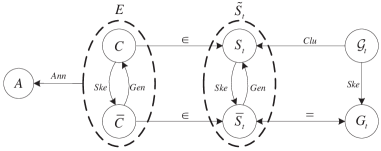
Figure 2: The functional relationships between different types of objects defined in this paper. Refer to Table 1 for notations.

In this paper, we introduce a sketch graph $G_{t}(V_{t},E_{t})$ of post network $\mathcal{G}_{t}(\mathcal{V}_{t},\mathcal{E}_{t})$ based on density parameters $(\delta_{1},\varepsilon_{0},\varepsilon_{1})$, where $\varepsilon_{1}\geq\varepsilon_{0}$. In density-based clustering , $\delta_{1}$ (a.k.a. $MinPts$ in DBSCAN [11]) is the minimum number of nodes in an $\varepsilon_{0}$-neighborhood, required to form a cluster. In the post network, we consider $\delta_{1}$ to be the threshold to judge whether a post is important and similarly $\varepsilon_{1}$ is a threshold for core edges. The reason we choose density-based clustering is that, compared with partitioning-based approaches (e.g., K-Means [14]) and hierarchical approaches (e.g., BIRCH [14]), density-based clustering (e.g., DBSCAN) defines clusters as areas of higher density than the remainder of the data set, which is effective in finding arbitrary-shaped clusters and is robust to noise. We adapt the concepts from density-based clustering and define the post weights as follows.

Definition 3

(Post Weight). Given a post $p=(L,\tau,a)$ in $\mathcal{G}_{t}(\mathcal{V}_{t},\mathcal{E}_{t})$ and its neighbor set $\mathcal{N}(p)$, the weight of $p$ at moment $t$, $\;t\geq p^{\tau}$, is defined as

$$w^{t}(p)=\frac{1}{D(|t-p^{\tau}|)}\sum_{q\in\mathcal{N}(p)}{S_{F}(p,q)}\vspace{-0.2cm}$$ (3)

Notice, post weight decays as time moves forward, although the neighbor set $\mathcal{N}(p)$ may change. Thus, post weights need to be continuously updated. In practice, we only store the sum $\sum_{q\in\mathcal{N}(p)}{S_{F}(p,q)}$ with $p$ to avoid frequent updates and compute $w^{t}(p)$ on demand when we need to judge the importance of a post. Based on post weight, we distinguish nodes in $\mathcal{G}_{t}(\mathcal{V}_{t},\mathcal{E}_{t})$ into three types, as defined below.

Definition 4

(Node Types).

• A post $p$ is a core post if $w^{t}(p)\geq\delta_{1}$;

• It is a border post if $w^{t}(p)<\delta_{1}$ but there exists at least one core post $q\in\mathcal{N}(p)$;

• It is a noise post if it is neither core nor border, i.e., $w^{t}(p)<\delta_{1}$ and there is no core post in $\mathcal{N}(p)$.

Intuitively, a post is a core post if it shares enough common entities with many other posts. Neighbors of a core post are at least border posts, if not core posts themselves. In density-based clustering, core posts play a central role: if a core post $p$ is found to be a part of a cluster $C$, its neighboring (border or core) posts will also be a part of $C$. Analogouly to the notion of core posts, we use the threshold $\delta_{1}$ to define core edges. An edge $(p,q)$ is a core edge if $S_{F}(p,q)\geq\varepsilon_{1}$, where $\varepsilon_{1}\geq\varepsilon_{0}$. Notice that a core edge may connect non-core nodes. Core posts connected by core edges will build a summary of $\mathcal{G}_{t}(\mathcal{V}_{t},\mathcal{E}_{t})$, that we call the sketch graph (See Figure 2).

Definition 5

(Sketch Graph). Given post network $\mathcal{G}_{t}(\mathcal{V}_{t},\mathcal{E}_{t})$ and density parameters $(\delta_{1},\varepsilon_{0},\varepsilon_{1})$, we define the sketch graph of $\mathcal{G}_{t}$ as the subgraph induced by its core posts and core edges. More precisely, the sketch graph $G_{t}(V_{t},E_{t})$ satisfies the condition that each node $p\in V_{t}$ is a core post and each edge $(p,q)\in E_{t}$ is a core edge. We write $G_{t}=Ske(\mathcal{G}_{t})$.

Intuitively, all important nodes in $\mathcal{G}_{t}(\mathcal{V}_{t},\mathcal{E}_{t})$ and their relationships are retained in $G_{t}(V_{t},E_{t})$. Empirically, we found that adjusting the granularity of $(\delta_{1},\varepsilon_{0},\varepsilon_{1})$ to make the size $|V_{t}|$ roughly equal to 20% of $|\mathcal{V}_{t}|$ leads to a good balance between the quality of the sketch graph in terms of the information retained and its space complexity. The tuning detail can be found in Section 7.1.

4.2 Event Identification and Annotation

We define events based on post clusters. Recall that if two core posts are connected by core edges, they should belong to the same cluster. It implies all core posts in cluster $C$ form a connected component $\overline{C}$ in $G_{t}(V_{t},E_{t})$ and we write $\overline{C}=Ske(C)$. Let $\overline{S_{t}}$ denote the set of connected components in $G_{t}$. Notice that $\overline{S_{t}}$ and $G_{t}$ have the same node set and the same structure, so we write $\overline{S_{t}}=G_{t}$ for simplicity. To generate clusters based on the sketch graph discussed above, we can start from a connected component $\overline{C}\in\overline{S_{t}}$ to build a cluster $C$. See Figure 2 for the functional relationships between different types of objects. We define cluster $C$ as follows.

Definition 6

(Cluster). Given $\mathcal{G}_{t}(\mathcal{V}_{t},\mathcal{E}_{t})$ and the corresponding sketch graph $G_{t}(V_{t},E_{t})$, a cluster $C$ of $\mathcal{G}_{t}$ is a set of core posts and border posts generated from a connected component $\overline{C}$ in $G_{t}(V_{t},E_{t})$, written as $C=Gen(\overline{C})$, and defined as follows:

• All posts in the component $\overline{C}$ form the core posts of $C$.

• For every core post in $C$, all its neighboring border posts in $\mathcal{G}_{t}$ form the border posts in $C$.

A core post only appears in one cluster (by definition). If a border post is associated with multiple core posts in different clusters, this border post will appear in multiple clusters. Events are defined based on clusters in $\mathcal{G}_{t}$. However, not every cluster can form an event; we treat clusters with a very small size as outliers, since they do not gain wide popularity at the current moment. We use $E$ and $O$ to denote an event and an outlier respectively.

Definition 7

(Event). Given a cluster $C$, the following function distinguishes between an event and an outlier.

$$Event(C)=\left\{\begin{matrix}{\bf true},\text{ if }|C|\geq\varphi\\ {\bf false},\text{ otherwise}\\ \end{matrix}\right.\vspace{-0.2cm}$$ (4)

where $\varphi$ is a size threshold.

We empirically set $\varphi=10$ for event identification. Note that outliers are different from noise; noise is associated at the level of posts, as opposed to clusters. Besides, an outlier at the current moment may grow into an event in the future, and an event may also degrade into an outlier as time passes.

Entity Annotation. Considering the huge volume of posts in an event, it is important to summarize and present a post cluster as a conceptual event to aid human perception. In related work, Twitinfo [22] represents an event it discovers from Twitter by a timeline of tweets. Although the tweet activity by volume over time is shown, it is tedious for users to read tweets one-by-one to figure out the event detail. In this paper, we summarize a snapshot of an event by a word cloud [13]. The font size of a word in the cloud indicates its popularity. Compared with Twitinfo, a word cloud provides a summary of the event at a glance and is much easier for a human to perceive. Technically, given an event $E$, the annotation $A$ for $E$, computed as $A=Ann(E)$, is a set of entities with popularity score, expressed as $A=\{(e_{1},P_{e_{1}}),(e_{2},P_{e_{2}}),\cdots\}$.

We take entities as the word candidates in the cloud. Intuitively, an entity $e$ is popular in an event if many important posts in this event contain $e$ in their entity list. Formally, the relationship between posts and entities can be modeled as a bipartite graph. Recall that the HITS algorithm [18] computes the hub score and authority score by mutual reinforcement: the hub score $\mathcal{H}_{i}$ of a node $i$ is decided by the sum of authority scores of all nodes pointed by $i$, and simultaneously, the authority score $\mathcal{A}_{j}$ of a node $j$ is decided by the sum of hub scores of all nodes pointing to $j$. Inspired by HITS, we let the post weight obtained from the post network be the initial hub score of posts, and then the authority scores of entities can be computed by one iteration: $\mathcal{A}=M^{T}\mathcal{H}$, where $M$ is an adjacency matrix between posts and entities in an event, $\mathcal{A}=[P_{e_{1}},P_{e_{2}},\cdots]^{T}$ is a vector of entity authorities and $\mathcal{H}=[w^{t}(p_{1}),w^{t}(p_{2}),\cdots]^{T}$ is a vector of post weights.

5 Tracking Event Evolution

In this section, we discuss the evolution of sketch graph and events and develop primitive operations, which form the theoretical basis for our algorithms in Section 6. We introduce the fading time window to serve as a monitor on social streams. Formally, the problem we try to solve in this paper is shown below.

Problem 1

Given an evolving post network sequence $\mathcal{G}=\{\mathcal{G}_{1},\mathcal{G}_{2},\cdots\}$, the event evolution tracking problem is to generate an event set $\widetilde{S}_{i}$ at each moment $i$, and discover all the evolution behaviors between events in $\widetilde{S}_{i}$ and $\widetilde{S}_{i+1}$, $\;i=1,2,\cdots$.

5.1 Incremental Tracking Framework

The traditional approach taken for tracking evolving network related problems [4, 16] is illustrated in Figure 3(a). Given a post network $\mathcal{G}_{t}$ at time $t$, identify the event set $\widetilde{S}_{t}$ associated with $\mathcal{G}_{t}$ (marked as step \raisebox{-.9pt} {1}⃝ in the figure). The network evolves from $\mathcal{G}_{t}$ to $\mathcal{G}_{t+1}$ at the next moment (step \raisebox{-.9pt} {2}⃝). Again, the events associated with $\mathcal{G}_{t+1}$ are identified from scratch (step \raisebox{-.9pt} {3}⃝). Finally, the correspondence between event sets $\widetilde{S}_{t}$ and $\widetilde{S}_{t+1}$ is determined to extract the evolution behaviors of events from time $t$ to $t+1$ (step \raisebox{-.9pt} {4}⃝). This traditional approach has two major shortcomings. Firstly, repeated extraction of events from post networks from scratch is an expensive operation. Similarly, tracing the correspondence between event sets at successive moments is also expensive. Secondly, this step of tracing correspondence, since it is done after the two event sets are generated, may lead to loss of accuracy. The method we propose is incremental tracking of event evolution. It corresponds to step \raisebox{-.9pt} {5}⃝ in the figure. More precisely, for the very first snapshot of the post network, say $\mathcal{G}_{0}$, our approach will generate the corresponding event set $\widetilde{S}_{0}$. After this, this step is never applied again. In the steady state, we apply step \raisebox{-.9pt} {5}⃝, i.e., we incrementally derive $\widetilde{S}_{t+1}$ from $\widetilde{S}_{t}$. Our experiments show that our incremental tracking approach outperforms the traditional baselines both in quality and in performance.

5.2 Evolution Operators

We analyze the evolutionary process of events at each moment and abstract them into five primitive operators: $+$, $-$, $\odot$, $\uparrow$, $\downarrow$. We classify the operators based on the objects they manipulate: nodes or clusters. Note that both events and outliers are clusters.

The following operators manipulate nodes in a post network.

Definition 8

(Node Operations).

• $\mathcal{G}_{t}+p$: add a new post $p$ into $\mathcal{G}_{t}(\mathcal{V}_{t},\mathcal{E}_{t})$ where $p\not\in\mathcal{V}_{t}$. All the new edges associated with $p$ will be constructed automatically by linkage search;

• $\mathcal{G}_{t}-p$: delete a post $p$ from $\mathcal{G}_{t}(\mathcal{V}_{t},\mathcal{E}_{t})$ where $p\in\mathcal{V}_{t}$. All the existing edges associated with $p$ will be automatically removed from $\mathcal{E}_{t}$.

• $\odot(\mathcal{G}_{t})$: update the weight of posts in $\mathcal{G}_{t}$.

Typically, the adding/deleting of a post will trigger the updating of post weights. For convenience, we define two composite operators on post networks.

Definition 9

(Composite Operators).

• $\mathcal{G}_{t}\oplus p=\odot(\mathcal{G}_{t}+p)$: add a post $p$ into $\mathcal{G}_{t}(\mathcal{V}_{t},\mathcal{E}_{t})$ where $p\not\in\mathcal{V}_{t}$ and update the weight of posts in $\mathcal{V}_{t}$;

• $\mathcal{G}_{t}\ominus p=\odot(\mathcal{G}_{t}-p)$: delete a post $p$ from $\mathcal{G}_{t}(\mathcal{V}_{t},\mathcal{E}_{t})$ where $p\in\mathcal{V}_{t}$ and update the weight of posts in $\mathcal{V}_{t}$.

The following operators manipulate clusters:

Definition 10

(Cluster Operations).

• $S_{t}+C$: add cluster $C$ to the cluster set $S_{t}$;

• $S_{t}-C$: remove cluster $C$ from the cluster set $S_{t}$;

• $\uparrow(C,p)$: increase the size of $C$ by adding a new post $p$;

• $\downarrow(C,p)$: decrease the size of $C$ by removing an old post $p$.

Each operator defined above on a single object can be extended to a set of objects, i.e., for a node set $\mathcal{X}=\{p_{1},p_{2},\cdots,p_{n}\}$, $\mathcal{G}_{t}+\mathcal{X}=\mathcal{G}_{t}+p_{1}+p_{2}+\cdots+p_{n}$. This is well defined since $+$ is associative and commutative.

We use the left-associative convention for ‘$-$’: that is, we write $A-B-C$ means $(A-B)-C$. In particular, we write $A-B+C$ to mean $(A-B)+C$ and the order in which posts in a set are added/deleted to $\mathcal{G}_{t}$ does not matter. These operators will be used later in the formal description of the evolution procedures. Figure 4 depicts the role played by the primitive operators in the event evolution tracking, end to end, from the post network onward.

5.3 Fading Time Window

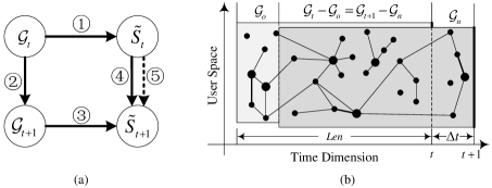
Figure 3: (a) Illustration of traditional approach vs. incremental approach to evolution tracking. Steps on edges are described in Section 5.1. (b) An illustration of the fading time window from time $t$ to $t+1$, where post weights fade w.r.t. the end of time window. $\mathcal{G}_{t}$ will be updated by deleting subgraph $\mathcal{G}_{o}$ and adding subgraph $\mathcal{G}_{n}$.

Fading (or decay) and sliding time window are two common aggregation schemes used in time-evolving graphs [9]. Fading scheme puts a higher emphasis on newer posts, and this characteristic has been captured by fading similarity in Eq. (1). Sliding time window scheme (posts are first-in, first-out) is essential because older posts are less important and it is not necessary to retain all the posts in the history. Since events evolve quickly, even inside a given time window, it is important to highlight new posts and degrade old posts using the fading scheme. Thus, we combine these two schemes and introduce a fading time window, as illustrated in Figure 3(b). In practice, users can specify the length of the time window to adjust the scope of monitoring. Users can also choose different fading functions to penalize old posts and highlight new posts in different ways. Let $\Delta t$ denote the interval between moments. For simplicity, we abbreviate the moment $(t+i\cdot\Delta t)$ as $(t+i)$. When the time window slides from moment $t$ to $t+1$, the post network $\mathcal{G}_{t}(\mathcal{V}_{t},\mathcal{E}_{t})$ will be updated to be $\mathcal{G}_{t+1}(\mathcal{V}_{t+1},\mathcal{E}_{t+1})$. Suppose $\mathcal{G}_{o}(\mathcal{V}_{o},\mathcal{E}_{o})$ is the old subgraph (of $\mathcal{G}_{t}$) that lapses at moment $t+1$ and $\mathcal{G}_{n}(\mathcal{V}_{n},\mathcal{E}_{n})$ is the new subgraph (of $\mathcal{G}_{t+1}$) that appears (see Figure 3(b)). Clearly,

$$\mathcal{G}_{t+1}=\mathcal{G}_{t}-\mathcal{G}_{o}+\mathcal{G}_{n}$$ (5)

Let $Len$ be the length of the time window. We assume $Len>2\Delta t$, which will make $\mathcal{V}_{o}\cap\mathcal{V}_{n}=\emptyset$. This assumption usually holds in real applications, e.g., we set $Len$ to 1 week and $\Delta t$ to 1 day. The following claim shows different ways to compute the overlapping part in $\mathcal{G}_{t+1}$ and $\mathcal{G}_{t}$.

Claim 1

$\mathcal{G}_{t+1}-\mathcal{G}_{n}=\mathcal{G}_{t}-\mathcal{G}_{o}=\mathcal{G}_{t+1}\ominus\mathcal{G}_{n}=\mathcal{G}_{t}\ominus\mathcal{G}_{o}$

Proof Sketch: From Eq. (5) we know $\mathcal{G}_{t+1}-\mathcal{G}_{n}=\mathcal{G}_{t}-\mathcal{G}_{o}$. At the post network level, post weight is orthogonal to node/edge sets, so we have $\mathcal{G}_{t}\ominus\mathcal{G}_{o}=\mathcal{G}_{t}-\mathcal{G}_{o}$ and $\mathcal{G}_{t+1}\ominus\mathcal{G}_{n}=\mathcal{G}_{t+1}-\mathcal{G}_{n}$.$\Box$

5.4 Sketch Graph Evolution

The updating of sketch graphs from $G_{t}$ to $G_{t+1}$ is the core task in event evolution tracking. We already know from Claim 1 that $\mathcal{G}_{t+1}-\mathcal{G}_{n}=\mathcal{G}_{t}-\mathcal{G}_{o}$ at the post network level. This is the overlapping part between $\mathcal{G}_{t}$ and $\mathcal{G}_{t+1}$. However, at the sketch graph level, $Ske(\mathcal{G}_{t+1}-\mathcal{G}_{n})\neq Ske(\mathcal{G}_{t}-\mathcal{G}_{o})$: some core posts in $\mathcal{G}_{t}-\mathcal{G}_{o}$ may no longer be core posts due to the removal of edges incident with nodes in $\mathcal{G}_{o}$ or simply due to the passing of time; some non-core posts may become core posts because of the adding of edges with nodes in $\mathcal{G}_{n}$. To measure the changes in the overlapping part, we define the following three components.

Definition 11

(Updated Components in Overlap).

• $\overline{S_{+}}$: components of non-core posts in $\mathcal{G}_{t}-\mathcal{G}_{o}$ that become core posts in $\mathcal{G}_{t+1}-\mathcal{G}_{n}$ due to the adding of $\mathcal{G}_{n}$, i.e.,

  $\overline{S_{+}}=Ske(\mathcal{G}_{t+1}-\mathcal{G}_{n})-Ske(\mathcal{G}_{t+1}\ominus\mathcal{G}_{n})$

• $\overline{S_{-}}$: components of core posts in $\mathcal{G}_{t}-\mathcal{G}_{o}$ that become non-core posts in $\mathcal{G}_{t+1}-\mathcal{G}_{n}$ due to the removing of $\mathcal{G}_{o}$, i.e.,

  $\overline{S_{-}}=Ske(\mathcal{G}_{t}-\mathcal{G}_{o})-Ske(\mathcal{G}_{t}\ominus\mathcal{G}_{o})$

• $\overline{S_{\odot}}$: components of core posts in $\mathcal{G}_{t}-\mathcal{G}_{o}$ that become non-core posts in $\mathcal{G}_{t+1}-\mathcal{G}_{n}$ due to the passing of time, i.e.,

  $\overline{S_{\odot}}=Ske(\mathcal{G}_{t}\ominus\mathcal{G}_{o})-Ske(\mathcal{G}_{t+1}\ominus\mathcal{G}_{n})$

Based on Definition 11, Theorem 1 shows how the overlapping parts in $\mathcal{G}_{t}$ and $\mathcal{G}_{t+1}$ differ at the sketch graph level.

Theorem 1

From moment $t$ to $t+1$, the changes of core posts in the overlapping part, i.e., $\mathcal{G}_{t+1}-\mathcal{G}_{n}$ (equivalently, $\mathcal{G}_{t}-\mathcal{G}_{o}$), can be updated using the components $\overline{S_{+}}$, $\overline{S_{-}}$ and $\overline{S_{\odot}}$. That is,

$$Ske(\mathcal{G}_{t+1}-\mathcal{G}_{n})-Ske(\mathcal{G}_{t}-\mathcal{G}_{o})=\overline{S_{+}}-\overline{S_{-}}-\overline{S_{\odot}}$$ (6)

Proof Sketch: $\overline{S_{+}}-\overline{S_{-}}-\overline{S_{\odot}}=Ske(\mathcal{G}_{t+1}-\mathcal{G}_{n})-Ske(\mathcal{G}_{t+1}\ominus\mathcal{G}_{n})-(Ske(\mathcal{G}_{t}-\mathcal{G}_{o})-Ske(\mathcal{G}_{t}\ominus\mathcal{G}_{o}))-(Ske(\mathcal{G}_{t}\ominus\mathcal{G}_{o})-Ske(\mathcal{G}_{t+1}\ominus\mathcal{G}_{n}))=Ske(\mathcal{G}_{t+1}-\mathcal{G}_{n})-Ske(\mathcal{G}_{t}-\mathcal{G}_{o})$. $\Box$

The following theorem shows the iterative and incremental updating of sketch graphs from moment $t$ to $t+1$.

Theorem 2

From moment $t$ to $t+1$, the sketch graph evolves by removing core posts in $\mathcal{G}_{o}$, adding core posts in $\mathcal{G}_{n}$ and updating core posts in the overlapping part. That is

$$\overline{S_{t+1}}={G}_{t+1}=\overline{S_{t}}-\overline{S_{o}}-\overline{S_{-}}-\overline{S_{\odot}}+\overline{S_{n}}+\overline{S_{+}}$$ (7)

Proof Sketch: $\overline{S_{+}}-\overline{S_{-}}-\overline{S_{\odot}}=Ske(\mathcal{G}_{t+1}-\mathcal{G}_{n})-Ske(\mathcal{G}_{t+1}\ominus\mathcal{G}_{n})-(Ske(\mathcal{G}_{t}-\mathcal{G}_{o})-Ske(\mathcal{G}_{t}\ominus\mathcal{G}_{o}))-(Ske(\mathcal{G}_{t}\ominus\mathcal{G}_{o})-Ske(\mathcal{G}_{t+1}\ominus\mathcal{G}_{n}))=Ske(\mathcal{G}_{t+1}-\mathcal{G}_{n})-Ske(\mathcal{G}_{t}-\mathcal{G}_{o})$. $\Box$

Theorem 2 indicates that we can incrementally maintain $\overline{S_{t+1}}$ from $\overline{S_{t}}$. Since we define events based on connected components in a sketch graph, this incremental updating of sketch graphs benefits incremental computation of event evolution essentially.

5.5 Event Evolution

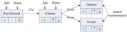
$|N_{c}(p)|$	0	1	$\geq 2$
Add a core post $p$	$+$	$\uparrow$	$Merge$
Delete a core post $p$	$-$	$\downarrow$	$Split$

Figure 4: (a) The relationships between primitives and evolutions. Each box represents an evolution object and the arrows between them describe inputs/outputs. (b) The evolutionary behavior table for clusters when adding or deleting a core post $p$.

Let $Clu(\mathcal{G}_{t})$ denote the clustering operation on post network $\mathcal{G}_{t}$. The clustering will shift and reorder the nodes in $\mathcal{V}_{t}$ by grouping nodes that belong to the same cluster together. We use $S_{t}=Clu(\mathcal{G}_{t})$ to represent the set of clusters obtained from $\mathcal{G}_{t}$. Notice that noise posts in $\mathcal{G}_{t}$ do not appear in any cluster, so the number of posts in $S_{t}$ is typically smaller than $|\mathcal{V}_{t}|$. Similarly, we let $Clu(\mathcal{G}_{n})=S_{n}$ and $Clu(\mathcal{G}_{o})=S_{o}$ be the cluster sets on the graphs $\mathcal{G}_{n}$ and $\mathcal{G}_{o}$.

Cluster Evolution. Based on Definition 6, a cluster at moment $t$ is generated from a component in $\overline{S_{t}}$. We can apply the $Gen$ function on sketch graphs to get the iterative computation of clusters.

Corollary 1

From moment $t$ to $t+1$, the set of clusters can be incrementally updated by the iterative computation

$${S_{t+1}}=Clu(\mathcal{G}_{t+1})={S_{t}}-{S_{o}}-{S_{-}}-{S_{\odot}}+{S_{n}}+{S_{+}}$$ (8)

Proof Sketch: Since the generation of any two clusters from two different components is independent, by applying $Gen$ function on both sides of Eq. (7) we get the iterative computation of clusters.$\Box$

The basic operations underlying Eq. (8) are the cases when $S_{t}$ is modified by the addition or deletion of a cluster that includes only one post. In the following, we analyze and show the evolution of clusters by adding a post $p_{n}$ or deleting a post $p_{o}$. Let $N_{c}(p_{n})$ denote the set of clusters where $p_{n}$’s neighboring core posts belong before $p_{n}$ is added, and let $N_{c}(p_{o})$ denote the set of clusters where $p_{o}$’s neighboring core posts belong after $p_{o}$ is removed. It should be noted that $|N_{c}(p)|=0$ means $p$ has no neighboring core posts. Notice that $Merge$ and $Split$ are composite operations and can be composed by a series of cluster primitive operations. The evolution behaviors of clusters is shown in Figure 4 and explained below.

(a) Addition: $S_{t}+\{p_{n}\}$

If $p_{n}$ is a noise post after being added into $\mathcal{G}_{t}$, ignore $p_{n}$. If $p_{n}$ is a border post, add $p_{n}$ to each cluster in $N_{c}(p_{n})$. Else, $p_{n}$ is a core post and we do the following:

• If $|N_{c}(p_{n})|=0$: $+C$ and $C=\{p_{n}\}\cup\mathcal{N}(p_{n})$;

• If $|N_{c}(p_{n})|=1$: $\uparrow(C,\{p_{n}\}\cup\mathcal{N}(p_{n}))$;

• If $|N_{c}(p_{n})|\geq 2$: $Merge=+C-\sum_{C^{\prime}\in N_{c}(p_{n})}{C^{\prime}}$ and $C=N_{c}(p_{n})\cup\{p_{n}\}\cup\mathcal{N}(p_{n})$.

(b) Deletion: $S_{t}-\{p_{o}\}$

If $p_{o}$ is a noise post before being deleted from $\mathcal{G}_{t}$, ignore $p_{o}$. If $p_{o}$ is a border post, delete $p_{o}$ from each cluster in $N_{c}(p_{o})$. Else, $p_{o}$ is a core post and we do the following:

• If $|N_{c}(p_{o})|=0$: $-C$ where $p_{o}\in C$;

• If $|N_{c}(p_{o})|=1$: $\downarrow(C,\{p_{o}\}\cup\mathcal{N}(p_{o}))$;

• If $|N_{c}(p_{o})|\geq 2$: $Split=-C+\sum_{C^{\prime}\in N_{c}(p_{o})}{C^{\prime}}$, $p_{o}\in C$.

Using commutativity and associativity of operator ‘$+$’ and the left-associative convention for operator ‘$-$’, we can rewrite the expression $S_{t}-p_{1}+p_{2}-p_{3}$ as $S_{t}-(p_{3}+p_{1})+p_{2}$. While both expressions are equivalent, in terms of the total number of primitive cluster operations, different ordering of cluster sequences may have different performance. In the following, we show a theorem to indicate how to reduce the number of primitive cluster operations by reordering. As an example, $S_{t}+p_{1}-p_{2}+p_{3}-p_{4}$ can be reordered as $S_{t}-(p_{2}+p_{4})+(p_{1}+p_{3})$ to reduce the number of primitive operations during cluster evolution.

Theorem 3

Suppose posts have an equal probability to join any cluster. Given an initial set of clusters and an arbitrary sequence of node addition and deletions, the number of cluster primitive operations can be reduced by performing all the deletions first.

Proof Sketch: Since posts have equal probability to join clusters, a smaller $|\mathcal{N}(p)|$ (i.e., the #edges of $p$) indicates a smaller number of neighboring clusters. Clearly, if the deletions are performed first, we can save time because there will be no edges between the deleted nodes and added nodes. Otherwise, the edges between the deleted nodes and added nodes need to be constructed first and removed later, which implies a higher $|\mathcal{N}(p)|$ in computation.$\Box$

The Evolution of Events and Outliers. Recall, at any moment, an outlier may grow into an event and an event may degrade into an outlier. Based on Definition 7, the evolution procedures of events and outliers follow the evolution of clusters. That is, the addition of a new event or outlier as well as the deletion of an existing event or outlier is exactly the same as for a cluster. The only difference is that the $Event$ function is applied to check whether the cluster added/deleted is an event or an outlier. When the size of a cluster increases (as with $\uparrow(C,p)$) it may correspond to an outlier/event growing into a larger outlier/event, or to an outlier growing in size, exceeding the threshold $\varphi$ and turning into an event. Similarly, when a cluster shrinks (as with $\downarrow(C,p)$) it may be an outlier/event becoming a smaller outlier/event or an event becoming smaller than the threshold and turning into an outlier.

6 Incremental Algorithms

The approach of decomposing an evolving graph into a series of snapshots for each moment is a traditional way to tackle evolving graph related problems [6, 16]. However, this traditional approach suffers from both quality and performance, since events are generated from scratch and are matched heuristically. To overcome these challenges, we propose an incremental tracking framework, as introduced in Section 5.1 and illustrated in Figure 3(a).

In this section, we leverage our primitive operators for evolution tracking by proposing Algorithms cTrack and eTrack to track the evolution of clusters and events respectively. The observation is that at each moment $|\mathcal{V}_{o}|+|\mathcal{V}_{n}|\ll|\mathcal{V}_{t}|$, where $\mathcal{V}_{o}$ and $\mathcal{V}_{n}$ are the set of old and new posts between moments $t$ and $t+1$. So we can save a lot of computation by adjusting clusters and events incrementally, rather than generating them from scratch.

Bulk Updating. Traditional incremental computation on evolving graphs usually treats the addition/deletion of nodes or edges one by one [10, 27]. In Section 5.5, we discussed the updating of $S_{t}$ by adding or deleting a single post. However, in a real scenario, since social posts arrive at a high speed, the post-by-post incremental updating will lead to poor performance. In this section, we speed up the incremental computation of $S_{t}$ by bulk updating. We define a bulk as a cluster of posts and “lift” the one-by-one updating of $S_{t}$ to bulk updating. Recall that $S_{n}$ and $S_{o}$ denote the set of clusters in the graph $\mathcal{G}_{n}=\mathcal{G}_{t+1}-\mathcal{G}_{t}$ and $\mathcal{G}_{o}=\mathcal{G}_{t}-\mathcal{G}_{t+1}$ respectively. Specifically, given a cluster $C_{n}\in S_{n}$, let $N_{c}(\overline{C_{n}})$ denote the set of clusters in $\mathcal{G}_{t}$ where neighboring core posts of nodes in $\overline{C_{n}}$ belong, i.e., $N_{c}(\overline{C_{n}})=\cup_{p_{n}\in\overline{C_{n}}}{N_{c}(p_{n})}$. Analogously, given $C_{o}\in S_{o}$, we let $N_{c}(\overline{C_{o}})=\cup_{p_{o}\in\overline{C_{o}}}{N_{c}(p_{o})}$. Clearly, updating $S_{t}$ with a single node $\{p\}$ is a special case of bulk updating.

cTrack. The steps for incremental tracking of cluster evolution (cTrack) are summarized in Algorithm 1. cTrack follows the iterative computation in Eq. (8) and sequence order in Theorem 3, that is ${S_{t+1}}={S_{t}}-{S_{o}}-{S_{-}}-{S_{\odot}}+{S_{n}}+{S_{+}}$. As analyzed in Section 5.5, each bulk addition and bulk deletion has three possible evolutionary behaviors, decided by the size of $N_{c}(\overline{C})$. Lines 3-13 deal with deleting a bulk $C_{o}$, where {$-$, $\downarrow$, $Split$} patterns are handled. Lines 15-27 deal with adding a bulk $C_{n}$ and handle {$+$, $\uparrow$, $Merge$} patterns. The time complexity of cTrack is linear in the total number of bulk updates.

Input: $S_{t}$, ${S}_{o}$, ${S}_{n}$, $S_{-}$, $S_{+}$, $S_{\odot}$

Output: $S_{t+1}$

1 $S_{t+1}=S_{t}$;

// Delete ${S}_{o}\cup S_{-}$

2 for each cluster $C_{o}$ in ${S}_{o}\cup S_{-}\cup S_{\odot}$ do

3       $\overline{C_{o}}=Ske(C_{o})$;

4       $N_{c}(\overline{C_{o}})=\cup_{p_{o}\in\overline{C_{o}}}{N_{c}(p_{o})}$;

5       if $|N_{c}(\overline{C_{o}})|=0$ then

6             remove cluster $C_{o}$ from $S_{t+1}$;

7            

8      else if $|N_{c}(\overline{C_{o}})|=1$ then

9             delete $C_{o}$ from cluster $C^{\prime}$ where $C^{\prime}\in N_{c}(\overline{C_{o}})$;

10            

11      else

12             remove the cluster that $C_{o}$ belongs to from $S_{t+1}$;

13             for each cluster $C^{\prime}\in N_{c}(\overline{C_{o}})$ do

14                   assign a new cluster id for $C^{\prime}$;

15                   add $C^{\prime}$ into $S_{t+1}$;

16                  

17            

18      

// Add ${S}_{n}\cup S_{+}$

19 for each cluster $C_{n}$ in ${S}_{n}\cup S_{+}$ do

20       $\overline{C_{n}}=Ske(C_{n})$;

21       $N_{c}(\overline{C_{n}})=\cup_{p_{n}\in\overline{C_{n}}}{N_{c}(p_{n})}$;

22       if $|N_{c}(\overline{C_{n}})|=0$ then

23             assign a new cluster id for $C_{n}$ and add $C$ to $S_{t+1}$;

24            

25      else if $|N_{c}(\overline{C_{n}})|=1$ then

26             add $C_{n}$ into cluster $C^{\prime}$ where $C^{\prime}\in N_{c}(\overline{C_{n}})$;

27            

28      else

29             assign a new cluster id for $C_{n}$;

30             for each cluster $C^{\prime}\in N_{c}(\overline{C_{n}})$ do

31                   $C_{n}=C_{n}\cup C^{\prime}$;

32                   remove $C^{\prime}$ from $S_{t+1}$;

33                  

34            $C_{n}=C_{n}\cup C_{n}$;

35             add $C_{n}$ into $S_{t+1}$;

36            

37      

38return $S_{t+1}$;

Algorithm 1 cTrack

eTrack. Algorithm eTrack works on top of cTrack. We summarize the steps for incremental event tracking (eTrack) in Algorithm 2. Based on cTrack, eTrack monitors the changes in the cluster set effected by cTrack at each moment. If the cluster is not changed, eTrack will take no action; otherwise, eTrack will judge the corresponding cases and invoke $Event$ function to handle the event evolution behaviors (Lines 4-13). Notice that in Lines 5-9, if a cluster $C$ in $S_{i}$ has ClusterId $id$, we use the convention that $S_{i}(id)=C$, and $S_{i}(id)=\emptyset$ means there is no cluster in $S_{i}$ with ClusterId $id$. Especially, lines 7-9 mean an event in $S_{i}$ evolves into an event in $S_{i+1}$ by deleting the part $S_{i}(id)-S_{i+1}(id)$ first and adding the part $S_{i+1}(id)-S_{i}(id)$ later.

Input: $\mathcal{G}=\{\mathcal{G}_{1},\mathcal{G}_{2},\cdots,\mathcal{G}_{n}\}$, $S_{1}$

Output: Event evolution behaviors

1 for $i$ from 1 to $n-1$ do

2       obtain ${S}_{o}$, ${S}_{n}$, $S_{-}$, $S_{+}$ from $\mathcal{G}_{i+1}-\mathcal{G}_{i}$;

3       $S_{i+1}=$cTrack $(S_{i},{S}_{o},{S}_{n},S_{-},S_{+},S_{\odot})$;

4       for each cluster $C\in S_{i+1}$ do

5             $id$ = $ClusterId(C)$;

6             if $S_{i}(id)\neq\emptyset$ then

7                   output $\downarrow(C,S_{i}(id)-S_{i+1}(id))$;

8                   output $\uparrow(C,S_{i+1}(id)-S_{i}(id))$;

9                   $Event(C)$;

10                  

11            else $Event(+C)$;

12            ;

13            

14      for each cluster $C\in S_{i}$ do

15             $id$ = $ClusterId(C)$;

16             if $S_{i+1}(id)=\emptyset$ then $Event(-C)$;

17            ;

18            

19      

Algorithm 2 eTrack

7 Experiments

In this section, we first “tune” the construction of post network and sketch graph to find the best selection of fading similarity measures and density parameters. Then, we test the quality and performance of event evolution tracking algorithms on two social streams: Tech-Lite and Tech-Full that we crawled from Twitter. We have designed two types of baseline algorithms for event detection and evolution tracking. Our event detection baseline covers the major techniques reported in [19, 22, 24, 25]. Our tracking baseline summarizes the state of the art algorithms reported in [6, 16]. All experiments are conducted on a computer with Intel 2.66 GHz CPU, 4 GB RAM, running 64-bit Windows 7. All algorithms are implemented in Java. We use a graph database called Neo4J to store and manipulate the post network and sketch graph.

Figure 5: Graph schemas of (a) post network and (b) sketch graph. Rectangles represent nodes and ellipses represent attributes. “Sim” means similarity edges between posts and “CoreSim” means core edges. “Weight” is the post weight. “ExpTime” is the time when a core post expires due to time passing. “Count” is the number of core posts in a component.

Figure 6: The changing trends of the number of core posts, core edges and events when increasing $\delta_{1}=\varepsilon_{1}$ from 0.3 to 0.8. We set $\delta_{1}=\varepsilon_{1}=0.3$ as the 100% basis and keep $\varepsilon_{0}=0.2$.

Datasets. All datasets are crawled from Twitter.com via Twitter API. Although our event tracking algorithm works regardless of the domain, we make the data set domain specific in order to facilitate evaluation of the generated results. We built a technology domain dataset called Tech-Lite by aggregating all the timelines of users listed in Technology category of “Who to follow” and their retweeted users. Tech-Lite has 352,328 tweets, 1402 users and the streaming rate is about 11700 tweets/day. Based on the intuition that users followed by users in Technology category are most likely also in the technology domain, we obtained a larger technology social stream called Tech-Full by collecting all the timelines of users that are followed by users in Technology category. Tech-Full has 5,196,086 tweets, created by 224,242 users, whose streaming rate is about 7216 tweets/hour. Both timelines in Tech-Lite and Tech-Full include retweets and have a time span from Jan. 1 to Feb. 1, 2012. Since Tech-Lite is a sampled subset of Tech-Full, the parameters learned from Tech-Lite generally apply to Tech-Full.

Graph Storage Schema. Neo4J provides convenience in managing a large and fast-evolving data structure that represents a post network and sketch graph. A database in Neo4J is based on the attributed graph model [26], where each node/edge can be associated with multiple attributes in the form of key-value pairs. Graph schemas of the post network and sketch graph are shown in Figure 5 (a) and (b) respectively. Indices are created on attributes to support fast exact queries and range queries of nodes.

7.1 Tuning Post Network and Sketch Graph

The quality of post network and sketch graph construction will determine the quality of event generation. Recall from Section 3 that the following factors influence the construction of post networks and sketch graphs: (1) entity extraction from post contents; (2) similarity/distance measures between posts; and (3) density parameters for the generation of core posts and core edges. We measure the influence of each factor below to make informed choices.

Post Content Preprocessing. As described in Section 3, we extract entities from posts by Stanford POS tagger. One alternative approach to entity extraction is using hashtags. However, only 11% of the tweets in our dataset have hashtags. This will result in lots of posts in the dataset having no similarity score between them. Another approach is simply tokenizing tweets into unigrams and treating unigrams as entities, and we call it the “Unigrams” approach. This approach is based on the state of art method for event detection as discussed in [22]. Table 2(a) shows the comparison of the three entity extraction approaches in the first time window of the Tech-Full social stream. If we use “Unigrams”, obviously the number of entities is larger than other two approaches, but the number of edges between posts tends to be smaller, because tweets written by different users usually share very few common words even when they talk about the same event. The “Hashtags” approach also produces a smaller number of edges, core posts and events, since it generates a much sparser post network. Overall, the “POS-Tagger” approach can discover more similarity relationships between posts and produce more core posts and events given the same social stream and parameter setting.

Methods	#edges	#coreposts	#coreedges	#events
Hashtags	182905	6232	28964	196
Unigrams	142468	15070	46783	430
POS-Tagger	357132	21509	47808	470

(a) Results of different entity extraction approaches.

Methods	#edges	#coreposts	#coreedges	#events
No-Fading	1159364	57291	32875	510
Exp-Fading	327390	7655	46075	148
Reci-Fading	357132	21509	47808	470

(b) Results of different distance functions.

Methods	Precision	Recall	Precision
	(major events)	(major events)	(G-Trends)
HashtagPeaks	0.40	0.30	0.25
UnigramPeaks	0.45	0.40	0.20
Louvain	0.60	0.55	0.75
eTrack	0.80	0.80	0.95

(c) Precision and recall of top 50 events.

Table 2: (a) and (b) are in the first time window of Tech-Lite with 75,849 posts in one week. Density parameters $(\delta_{1},\varepsilon_{0},\varepsilon_{1})=(0.5,0.2,0.5)$ for core posts and threshold $\varphi=10$ for event identification. (c) shows the precision and recall of top 20 events generated by Baseline 1a, 1b, Louvain and eTrack.

Similarity/Distance Measures. Many set-based similarity measures such as Jaccard coefficient [21] can be used to compute the similarity $S(p_{i}^{L},p_{j}^{L})$ between posts. Since entity frequency is usually 1 in a tweet, measures such as Cosine similarity and Pearson correlation [21] will degenerate to a form very similar to Jaccard, so we use Jaccard. The distance function $D(|p_{i}^{\tau}-p_{j}^{\tau}|)$ along time dimension determines how similarity to older posts is penalized, with respect to recent posts. We compared three different distance functions: (1) reciprocal fading (“Reci-Fading”) with $D(|p_{i}^{\tau}-p_{j}^{\tau}|)={|p_{i}^{\tau}-p_{j}^{\tau}|+1}$, (2) exponential fading (“Exp-Fading”) with $D(|p_{i}^{\tau}-p_{j}^{\tau}|)={e^{|p_{i}^{\tau}-p_{j}^{\tau}|}}$ and (3) no fading (“No-Fading”) with $D(|p_{i}^{\tau}-p_{j}^{\tau}|)=1$. For any posts $p_{i},p_{j}$, clearly $e^{|p_{i}^{\tau}-p_{j}^{\tau}|}\geq{|p_{i}^{\tau}-p_{j}^{\tau}|+1}\geq 1$. Since a time window usually contains many moments, Exp-Fading penalizes the posts in the old part of time window severely (see Table 2(b)): the number of core posts and events generated by Exp-Fading is much lower than by other approaches. Since No-Fading does not penalize old posts in the time window, too many edges and core posts will be generated without considering recency. Reci-Fading is in between, which is a more gradual penalty function than Exp-Fading and we use it by default.

Density Parameters. The density parameters $(\delta_{1},\varepsilon_{0},\varepsilon_{1})$ control the construction of the sketch graph. Clearly, the higher the density parameters, the smaller and sparser the sketch graph. Figure 6 shows the number of core posts, core edges and events as a percentage of the numbers for $\delta_{1}=\varepsilon_{1}=0.3$, as $\delta_{1}=\varepsilon_{1}$ increases from 0.3 to 0.8. Results are obtained from the first time window of the Tech-Lite social stream. We can see the rate of decrease of $\#$events is higher than the rates of $\#$core posts and $\#$core edges, because events are less likely to form in sparser sketch graphs. More small events can be detected by lower density parameters, but the computational cost will increase because of larger and denser sketch graphs. However, for big events, they are not very sensitive to these density parameters. We set $\delta_{1}=\varepsilon_{1}=0.5$ as a trade-off between the compactness of events and complexity.

7.2 Event Evolution Tracking

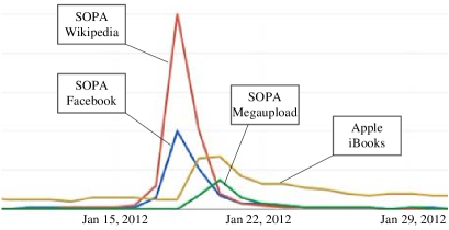
Figure 7: Examples of Google Trends peaks in January 2012. We validate the events generated by cTrack by checking the existence of volume peaks at a nearby time moment in Google Trends. Although these peaks can detect bursty events, Google Trends cannot discover the merging/splitting patterns.

Figure 8: Lists of top 10 events detected from Twitter Technology streams in January 2012 by baseline HashtagPeaks, UnigramPeaks, Louvain and our approach eTrack. To adapt for event detection, Louvain method defines events by post communities. We annotate events generated by both Louvain and eTrack by highly frequent entities. eTrack also shows the birthday of events.

Ground truth. To generate the ground truth, we crawl news articles in January 2012 from famous technology websites such as TechCrunch, Wired, CNET, etc, without looking at tweets. Then we treat the titles of news as posts and apply our event tracking algorithm to extract event evolution patterns. Finally, a total of 20 major events with life cycles are identified as ground truth. Typical events include “happy new year”, “CES 2012”, “jerry yang yahoo resignation”, “sopa wikipedia blackout”, etc.

To find more noticeable events in the technology news domain, we use Google Trends for Search, which shows the traffic trends of keywords that appeared in Google Search along the time dimension. If an event-indicating phrase has a volume peak in Google Trends at a specific time, it means this event is sufficiently validated by the real world. We validate the correctness of an event $E_{i}$ generated by our approach by the following process: we pick the top 3 entities of $E_{i}$ ranked by frequency in $E_{i}$ and search them in Google Trends, and if the traffic trend of these top entities has a distinct peak at a nearby time to $E_{i}$, we consider that $E_{i}$ corresponds to a real world event widely witnessed by the public. Four examples of Google Trends peaks are shown in Figure 7.

Baseline 1: Peak-Detection. In recent works [19, 22, 24, 25], events are generally detected as volume peaks of phrases over time in social streams. These approaches share the same spirit that aggregates the frequency of event-indicating phrases at each moment to build a histogram and generates events by detecting volume peaks in the histogram. We design two variants of Peak-Detection to capture the major techniques used by these state-of-the-art approaches.

• Baseline 1a: HashtagPeaks: aggregates frequent hashtags;

• Baseline 1b: UnigramPeaks: aggregates frequent unigrams.

Notice, both baselines above are for event detection only. Lists of the top 10 events detected by HashtagPeaks and UnigramPeaks are presented in Figure 8 (first two columns). Hashtags are employed by twitter users as a manual way to indicate an event, but it requires manual assignation by a human. Some highly frequent hashtags like “#opengov” and “#opendata” are not designed for event indication, hurting the precision. UnigramPeaks uses the entities extracted from the social stream preprocessing stage, which has a better quality than HashtagPeaks. However, both of them are limited in their representation of events, because the internal structure of events is missing. Besides, although these peaks can detect bursty words, they cannot discover evolution patterns such as the merging/splitting of events. For example, in Figure 7, there is no way to know “Apple announced iBooks” is an event split from the big event “SOPA” earlier, as illustrated in detail in Figure 9(b).

Baseline 2: Community Detection. A community in a large network refers to a structure of nodes with dense connections internally and sparse connections between communities. It is possible to define an event as a community of posts. Louvain method [8], based on modularity optimization, is the state-of-the-art approach which outperforms other known community detection methods in terms of performance. We design a baseline called “Louvain” to detect events defined as post communities.

The top 10 events generated by Louvain are shown in Figure 8. As we can see, not every result is meaningful in Louvain method. For example, “Apple iphone ipad” and “Internet people time” are too vague to correspond to any concrete real events. The reason is, although Louvain method can make sure every community has relatively dense internal and sparse external connections, it cannot guarantee that every node in the community is important and has a sufficiently high connectivity with other nodes in the same community. It is highly possible that a low-degree node belongs to a community only because it has zero connectivity with other communities. Furthermore, noise posts are quite prevalent in Twitter and they negatively impact Louvain method.

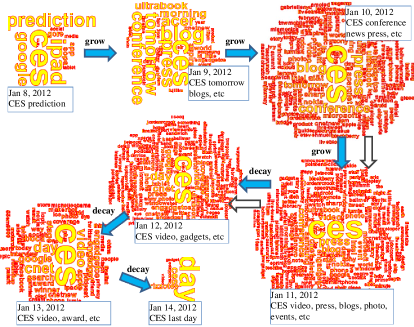
(a) The life cycle of “CES Conference”

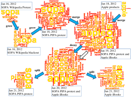
(b) The merging and splitting of “SOPA” and “Apple”

Figure 9: Tracking the evolution of events by eTrack and baselines. At each moment, an event is annotated by a word cloud. Baselines 1 and 2 only works for the detection of new emerging events, and is not applicable for the tracking of merging and splitting dynamics. The evolution trajectories of eTrack and Baseline 3 are depicted by solid and hollow arrows respectively.

Baseline 3: Pattern-Matching. We design a baseline to track the evolution patterns of events between snapshots. In graph mining, the “divide-and-conquer” approach of decomposing the evolving graph into a series of snapshot graphs at each moment is a traditional way to tackle evolving graph related problems [6, 16]. As an example, Kim et al. [16] first cluster individual snapshots into quasi-cliques and then map them in adjacent snapshots over time. Inspired by this approach, we design a baseline for event evolution tracking, which detects events from each snapshot of post network independently, and then characterizes the evolution of these events at consecutive moments, by identifying certain heuristic patterns:

$\bullet$ If $\frac{|E_{t}\cap E_{t+1}|}{|E_{t}\cup E_{t+1}|}\geq\kappa\%$ and $|E_{t}|\leq|E_{t+1}|$, $E_{t+1}=\uparrow E_{t}$;

$\bullet$ If $\frac{|E_{t}\cap E_{t+1}|}{|E_{t}\cup E_{t+1}|}\geq\kappa\%$ and $|E_{t}|>|E_{t+1}|$, $E_{t+1}=\downarrow E_{t}$.

where $E_{t}$ and $E_{t+1}$ are any two events detected at moment $t$ and $t+1$ respectively, $\kappa\%$ is the minimal commonality to say $E_{t}$ and $E_{t+1}$ are snapshots of the same event. A higher $\kappa\%$ will result in a higher precision but a lower recall of the evolution tracking. Empirically we found that we needed to set $\kappa\%=90\%$ to guarantee the quality. It is worth noting that this baseline generates the same events as eTrack, but with a non-incremental evolution tracking approach.

Precision and Recall. To measure the quality of event detection, we use HashtagPeaks, UnigramPeaks and Louvain as baselines to compare with our Algorithm eTrack. It is worth noting that Baseline 3 is designed for the tracking of event evolution dynamics between moments, so we omit it here. We compare the precision and recall of top 20 events generated by baselines and eTrack and show the results in Table 2(c). On the ground truth of 20 major events obtained from news articles in technology websites, HashtagPeaks and UnigramPeaks have rather low precision and recall scores, because of their poor ability in capturing event bursts. Notice that the precision and recall may be not equal even the sizes of extracted events and ground truth are equal, because multiple extracted events may correspond to the same event in ground truth. eTrack outperforms the baselines in both precision and recall. Since there are many events discussed in the social media but not very noticeable in news websites, we also validate the precision of the generated events using Google Trends. As we can see, HashtagPeaks and UnigramPeaks don’t gain too much in Google Trends validation, since the words they generate are less informative and not very event-indicating. eTrack gains a precision of 95% in Google Trends, where the only failed result is “Samsung galaxy nexus”, whose volume is steadily high without obvious peaks in Google Trends. The reason may be social stream is more dynamic. Louvain is worse than eTrack. The results show eTrack is significantly better than other baselines in quality.

Life Cycle of Event Evolution. Our approach is capable of tracking the whole life cycle of an event: from birth, growth, decay to death. We illustrate this using the example of “CES 2012”, a major consumer electronics show held in Las Vegas from January 10 to 13. As early as Jan 6, our approach has already detected some discussions about CES and generated an event about CES. Figure 9(a) shows the major snapshots of this event, from Jan 8 to Jan 14. As we can see, on Jan 8, most people talked about “CES prediction”, and on Jan 9, the highlighted topic was “CES tomorrow” and some hearsays about “ultrabook” which would be shown in CES. After the actual event happened on Jan 10, we can see the event grew distinctly bigger, and lots of products, news and messages are spreading over the social network, and this situation continues until Jan 13, which is the last day of CES. Afterwards, the discussions become weaker and continue until Jan 14, when “CES” was not the biggest mention on that day but still existed in some discussions. Compared with our approach, Baselines 1 and 2 can detect the emerging of “CES” with a frequency count at each moment, but no trajectory is generated. Baseline 3 can track a very coarse trajectory of this event, i.e., from Jan 10 to Jan 12. The reason is, if an event changes rapidly and many posts at consecutive moments cannot be associated with each other, Baseline 3 will fail to track the evolution. Since in social streams the posts usually surge quickly, our approach is superior over the baselines.

Event Merging & Splitting. Figure 9(b) illustrates an example of event merging and splitting generated by Algorithm eTrack. eTrack detected the event of SOPA (Stop Online Piracy Act) and Wikipedia on Jan 16, because on that day Wikipedia announced the blackout on Wednesday (Jan 18) to protest SOPA. This event grew distinctly on Jan 17 and Jan 18, by inducing more people in the social network to discuss about this topic. At the same time, there was another event detected on Jan 18, discussing Apple’s products. On Jan 19, actually the SOPA event and Apple event were merged, because Apple joined the SOPA protest and lots of Apple products such as iBooks in education are actually directly related to SOPA. This event evolved on Jan 20, by adding more discussions about iBooks 2. Apple iBooks 2 was actually unveiled in Jan 21, while this new product gained lots of attention, people who talked about iBooks did not talk about SOPA anymore. Thus, on Jan 21, the SOPA-Apple event was split into two events, which would evolve independently afterwards. Unfortunately, the above merging and splitting process cannot be tracked by any of the baselines, which output some independent events. The reason for Baseline 3 is, given the ground truth $E_{t+1}=E_{t1}+E_{t2}$, i.e., $E_{t1}$ and $E_{t2}$ merged into $E_{t+1}$, $\frac{|E_{t1}\cap E_{t+1}|}{|E_{t1}\cup E_{t+1}|}\geq\kappa\%$ or $\frac{|E_{t2}\cap E_{t+1}|}{|E_{t2}\cup E_{t+1}|}\geq\kappa\%$ is most likely invalid, so the ground truth cannot be tracked.

(a) Varying time window

(b) Varying step length

Figure 10: The running time on two datasets as the adjusting of the time window length and step length.

7.3 Running Time

We measure how the baseline and eTrack scale w.r.t. both the varying time window width and the step length. We use both Tech-Lite and Tech-Full streams, and set the time step interval $\Delta t=1$ day for Tech-Lite, $\Delta t=1$ hour for Tech-Full to track events on different time granularity. The streaming post rates for Tech-Lite and Tech-Full are 11700/day and 7126/hour respectively. Figure 10(a) shows the running time of eTrack when we increase the time window length, and we can see for a time window of $10\Delta t$ hours in Tech-Full, our approach can finish the post preprocessing, post network construction and event tracking in just 3 minutes. A key observation is that the running time of eTrack does not depend on the overall size of the dataset. Rather, it depends on the streaming speed of posts in $\Delta t$. Figure 10(b) shows if we fix the time window length as $10\Delta t$ and increase the step length of the sliding time window, the running time of eTrack grows nearly linearly. Compared with our incremental computation, Baseline 3 has to process posts in the whole time window from scratch at each moment, so the running time will be steadily high. If the step length is larger than $4\Delta t$ in TechFull, eTrack does not have an advantage in running time compared with Baseline 3, because a large part of post network is updated at each moment. However, this extreme case is rare. Since in a real scenario, the step length is much smaller than the time window length, our approach shows much better efficiency than the baseline approach.

8 Conclusion

Our main goal in this paper is to track the evolution of events over social streams such as Twitter. To that end, we extract meaningful information from noisy post streams and organize it into an evolving network of posts under a sliding time window. We model events as sufficiently large clusters of posts sharing the same topics, and propose a framework to describe event evolution behaviors using a set of primitive operations. Unlike previous approaches, our evolution tracking algorithm eTrack performs incremental updates and efficiently tracks event evolution patterns in real time. We experimentally demonstrate the performance and quality of our algorithm over two real data sets crawled from Twitter. As a natural progression, in the future, it would be interesting to investigate the tracking of evolution of social emotions on products, with its obvious application for business intelligence.

References

- [1] The guardian: Average twitter user has 126 followers. http://www.guardian.co.uk/technology/blog/2009 /jun/29/twitter-users-average-api-traffic.
- [2] M. K. Agarwal, K. Ramamritham, and M. Bhide. Real time discovery of dense clusters in highly dynamic graphs: Identifying real world events in highly dynamic environments. PVLDB, 5(10):980–991, 2012.
- [3] C. C. Aggarwal, J. Han, J. Wang, and P. S. Yu. A framework for clustering evolving data streams. In VLDB, pages 81–92, 2003.
- [4] J. Allan, editor. Topic detection and tracking: event-based information organization. Kluwer Academic Publishers, 2002.
- [5] A. Angel, N. Koudas, N. Sarkas, and D. Srivastava. Dense subgraph maintenance under streaming edge weight updates for real-time story identification. PVLDB, 5(6):574–585, 2012.
- [6] S. Asur, S. Parthasarathy, and D. Ucar. An event-based framework for characterizing the evolutionary behavior of interaction graphs. In KDD, pages 913–921, 2007.
- [7] H. Becker, M. Naaman, and L. Gravano. Learning similarity metrics for event identification in social media. In WSDM, pages 291–300, 2010.
- [8] V. Blondel, J.-L. Guillaume, R. Lambiotte, and E. Lefebvre. Fast unfolding of communities in large networks. J. Stat. Mech., P10008, 2008.
- [9] F. Cao, M. Ester, W. Qian, and A. Zhou. Density-based clustering over an evolving data stream with noise. In SDM, 2006.
- [10] Y. Chen and L. Tu. Density-based clustering for real-time stream data. In KDD, pages 133–142, 2007.
- [11] M. Ester, H.-P. Kriegel, J. Sander, and X. Xu. A density-based algorithm for discovering clusters in large spatial databases with noise. In KDD, pages 226–231, 1996.
- [12] G. P. C. Fung, J. X. Yu, P. S. Yu, and H. Lu. Parameter free bursty events detection in text streams. In VLDB, pages 181–192, 2005.
- [13] M. Halvey and M. T. Keane. An assessment of tag presentation techniques. In WWW, pages 1313–1314, 2007.
- [14] J. Han, M. Kamber, and J. Pei. Data Mining: Concepts and Techniques. Morgan Kaufmann, 2011.
- [15] X. Jin, W. S. Spangler, R. Ma, and J. Han. Topic initiator detection on the world wide web. In WWW, pages 481–490, 2010.
- [16] M.-S. Kim and J. Han. A particle-and-density based evolutionary clustering method for dynamic networks. PVLDB, 2(1):622–633, 2009.
- [17] D. Klein and C. D. Manning. Accurate unlexicalized parsing. In ACL, pages 423–430, 2003.
- [18] J. M. Kleinberg. Authoritative sources in a hyperlinked environment. J. ACM, 46(5):604–632, 1999.
- [19] J. Leskovec, L. Backstrom, and J. M. Kleinberg. Meme-tracking and the dynamics of the news cycle. In KDD, pages 497–506, 2009.
- [20] B. Liu, C. W. Chin, and H. T. Ng. Mining topic-specific concepts and definitions on the web. In WWW, pages 251–260, 2003.
- [21] C. D. Manning, P. Raghavan, and H. Schuetze. Introduction to Information Retrieval. Cambridge University Press, 2008.
- [22] A. Marcus, M. S. Bernstein, O. Badar, D. R. Karger, S. Madden, and R. C. Miller. Twitinfo: aggregating and visualizing microblogs for event exploration. In CHI, pages 227–236, 2011.
- [23] D. Nadeau and S. Sekine. A survey of named entity recognition and classification. Lingvisticae Investigationes, 30(1):3–26, 2007.
- [24] T. Sakaki, M. Okazaki, and Y. Matsuo. Earthquake shakes twitter users: real-time event detection by social sensors. In WWW, pages 851–860, 2010.
- [25] A. D. Sarma, A. Jain, and C. Yu. Dynamic relationship and event discovery. In WSDM, pages 207–216, 2011.
- [26] S. Srinivasa. Data, storage and index models for graph databases. In Graph Data Management, pages 47–70. 2011.
- [27] L. Wan, W. K. Ng, X. H. Dang, P. S. Yu, and K. Zhang. Density-based clustering of data streams at multiple resolutions. TKDD, 3(3), 2009.
- [28] J. Weng and B.-S. Lee. Event detection in twitter. In ICWSM, 2011.
- [29] Y. Yang, T. Ault, T. Pierce, and C. W. Lattimer. Improving text categorization methods for event tracking. In SIGIR, pages 65–72, 2000.